Introduction - Weizmann Institute of Science
21
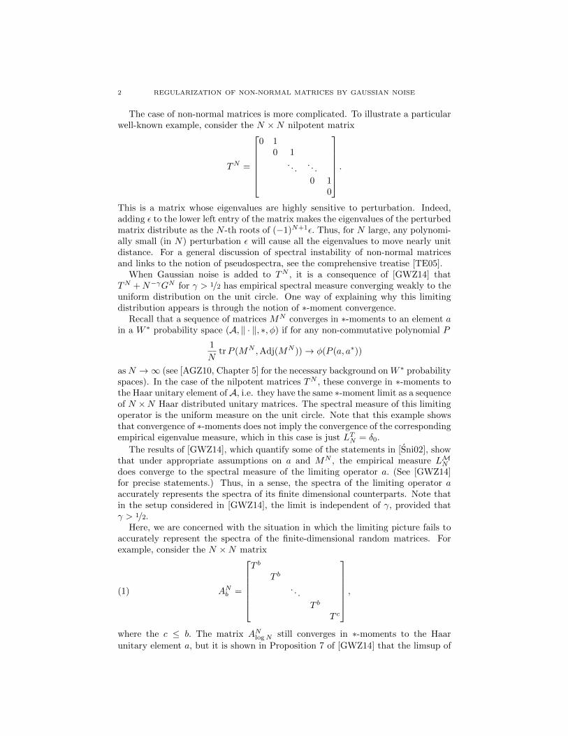
REGULARIZATION OF NON-NORMAL MATRICES BY GAUSSIAN NOISE OHAD FELDHEIM, ELLIOT PAQUETTE, AND OFER ZEITOUNI Abstract. We consider the regularization of matrices M N written in Jordan form by additive Gaussian noise N -γ G N , where G N is a matrix of i.i.d. stan- dard Gaussians and γ> 1 /2 so that the operator norm of the additive noise tends to 0 with N . Under mild conditions on the structure of M N we evaluate the limit of the empirical measure of eigenvalues of M N + N -γ G N and show that it depends on γ, in contrast with the case of a single Jordan block. 1. Introduction Write G N for an N ×N random matrix whose entries are i.i.d. Gaussian variables, and let {M N } ∞ N=1 be a sequence of deterministic N × N matrices. Consider a noisy counterpart given by M N = M N + N -γ G N , where γ ∈ (0, ∞) is fixed. It is natural to ask how the spectra of M N differs from the spectra of M N . To meaure this, define the empirical spectral measure of M N as L M N := 1 N N X i=1 δ λi (M N ) where λ i (M N ),i =1,...,N are the eigenvalues of M N , and δ x is the Dirac mass at x. If {M N } are normal, then when γ> 1 / 2,L M N - L M N converges weakly in proba- bility to 0 as N →∞. This follows immediately from Theorem 1.1 of [Sun96] and the observation that the operator norm of N -γ G N goes to 0 in probability if and only if γ> 1 / 2. This is one precise sense in which normal matrices are stable under perturbation. See also [Bha97] for more background on the stability of the spectra of normal matrices. Department of Mathematics, Weizmann Institute of Science Department of Mathematics, Weizmann Institute of Science Department of Mathematics, Weizmann Institute of Science E-mail addresses: ohad [email protected], [email protected], [email protected]. Date : April 13, 2014. Partially supported by an ISF grant and by the Herman P. Taubman chair of Mathematics at the Weizmann Institute. EP gratefully acknowledges the support of NSF Postdoctoral Fellowship DMS-1304057. 1
Transcript of Introduction - Weizmann Institute of Science
REGULARIZATION OF NON-NORMAL MATRICES BY
GAUSSIAN NOISE
OHAD FELDHEIM, ELLIOT PAQUETTE, AND OFER ZEITOUNI
Abstract. We consider the regularization of matrices MN written in Jordanform by additive Gaussian noise N−γGN , where GN is a matrix of i.i.d. stan-
dard Gaussians and γ > 1/2 so that the operator norm of the additive noise
tends to 0 with N . Under mild conditions on the structure of MN we evaluatethe limit of the empirical measure of eigenvalues of MN +N−γGN and show
that it depends on γ, in contrast with the case of a single Jordan block.
1. Introduction
WriteGN for anN×N random matrix whose entries are i.i.d. Gaussian variables,and let MN∞N=1 be a sequence of deterministic N×N matrices. Consider a noisycounterpart given by
MN = MN +N−γGN ,
where γ ∈ (0,∞) is fixed.It is natural to ask how the spectra of MN differs from the spectra of MN . To
meaure this, define the empirical spectral measure of MN as
LMN :=1
N
N∑i=1
δλi(MN )
where λi(MN ), i = 1, . . . , N are the eigenvalues of MN , and δx is the Dirac mass
at x.If MN are normal, then when γ > 1/2, LMN − LMN converges weakly in proba-
bility to 0 as N → ∞. This follows immediately from Theorem 1.1 of [Sun96] andthe observation that the operator norm of N−γGN goes to 0 in probability if andonly if γ > 1/2. This is one precise sense in which normal matrices are stable underperturbation. See also [Bha97] for more background on the stability of the spectraof normal matrices.
Department of Mathematics, Weizmann Institute of ScienceDepartment of Mathematics, Weizmann Institute of Science
Department of Mathematics, Weizmann Institute of ScienceE-mail addresses: ohad [email protected], [email protected],
Date: April 13, 2014.Partially supported by an ISF grant and by the Herman P. Taubman chair of Mathematics at
the Weizmann Institute. EP gratefully acknowledges the support of NSF Postdoctoral FellowshipDMS-1304057.
1
2 REGULARIZATION OF NON-NORMAL MATRICES BY GAUSSIAN NOISE
The case of non-normal matrices is more complicated. To illustrate a particularwell-known example, consider the N ×N nilpotent matrix
TN =
0 1
0 1. . .
. . .
0 10
.This is a matrix whose eigenvalues are highly sensitive to perturbation. Indeed,adding ε to the lower left entry of the matrix makes the eigenvalues of the perturbedmatrix distribute as the N -th roots of (−1)N+1ε. Thus, for N large, any polynomi-ally small (in N) perturbation ε will cause all the eigenvalues to move nearly unitdistance. For a general discussion of spectral instability of non-normal matricesand links to the notion of pseudospectra, see the comprehensive treatise [TE05].
When Gaussian noise is added to TN , it is a consequence of [GWZ14] thatTN +N−γGN for γ > 1/2 has empirical spectral measure converging weakly to theuniform distribution on the unit circle. One way of explaining why this limitingdistribution appears is through the notion of ∗-moment convergence.
Recall that a sequence of matrices MN converges in ∗-moments to an element ain a W ∗ probability space (A, ‖ · ‖, ∗, φ) if for any non-commutative polynomial P
1
NtrP (MN ,Adj(MN ))→ φ(P (a, a∗))
as N →∞ (see [AGZ10, Chapter 5] for the necessary background on W ∗ probabilityspaces). In the case of the nilpotent matrices TN , these converge in ∗-moments tothe Haar unitary element ofA, i.e. they have the same ∗-moment limit as a sequenceof N ×N Haar distributed unitary matrices. The spectral measure of this limitingoperator is the uniform measure on the unit circle. Note that this example showsthat convergence of ∗-moments does not imply the convergence of the correspondingempirical eigenvalue measure, which in this case is just LTN = δ0.
The results of [GWZ14], which quantify some of the statements in [Sni02], showthat under appropriate assumptions on a and MN , the empirical measure LMNdoes converge to the spectral measure of the limiting operator a. (See [GWZ14]for precise statements.) Thus, in a sense, the spectra of the limiting operator aaccurately represents the spectra of its finite dimensional counterparts. Note thatin the setup considered in [GWZ14], the limit is independent of γ, provided thatγ > 1/2.
Here, we are concerned with the situation in which the limiting picture fails toaccurately represent the spectra of the finite-dimensional random matrices. Forexample, consider the N ×N matrix
(1) ANb =
T b
T b
. . .
T b
T c
,where the c ≤ b. The matrix ANlogN still converges in ∗-moments to the Haar
unitary element a, but it is shown in Proposition 7 of [GWZ14] that the limsup of
REGULARIZATION OF NON-NORMAL MATRICES BY GAUSSIAN NOISE 3
the spectral radius ANlogN + N−γGN is strictly smaller than 1, if γ > γ0 for somefixed γ0.
In this paper, we show that a natural class of matrices generalizing ANlogN , when
perturbed by Gaussian noise N−γGN , have empirical measures of eigenvalues con-verging to γ-dependent limits.
Definitions and main results. For each N , let Bi(N)`(N)i=1 be a family of Jor-
dan blocks, with Bi = Bi(N) having dimension ai logN where ai = ai(N) and∑`(N)i=1 ai logN = N . We denote by ci = ci(N) the eigenvalue of Bi.Introduce the matrix
MN =
B1
B2
. . .
B`(N)
.Fix γ > 1/2 and consider the matrix M = MN + N−γGN , where GN is a matrixof i.i.d. standard normal variables. Our main result gives the convergence of theempirical distribution of eigenvalues of M.
To describe the limit, let ri = ri(N) = exp((−γ+1/2)/ai). Let mc,r be the uniformprobability measure on the circle centered at c with radius r. Let LN denote theempirical spectral measure of MN . Set µN to be the measure on C given by
µN :=
`(N)∑i=1
ai logN
Nmci,ri .
If γ > 1, we show that µN converges to µ provided ` = o(N).
Theorem 1.1. Suppose that γ > 1 and `(N) = o(N). Suppose further that thereis a compact K ⊆ C so that all µN are supported on K, and suppose that thereis a probability measure µ so that µN ⇒ µ. Then, the empirical measure LN ofMN +N−γGN converges to µ weakly in probability.
Remark 1.2. If the sequence µN is tight but not necessarily convergent, onecould rephrase Theorem 1.1 as the statement that d(LN , µN ) →N→∞ 0 in proba-bility, where d is any metric compatible with weak convergence.
Theorem 1.1 is an immediate consequence of our main result, Theorem 1.4 below,which handles also the case γ ∈ (1/2, 1] at the cost of imposing an extra condition,essentially that circles arising from polynomially large blocks cover only a smallportion of the plane; we now make this extra condition precise.
Fix ε′ > 0 satisfying ε′ < 2γ − 1. Set
VN = VN (ε′) =z ∈ C : ∀i ∈ [`(N)],min(ai log(N), |1− |z − ci|2|−1) < N2γ−1−ε′
and
V = V(ε′) :=
∞⋃N=k
∞⋂k=1
VN .
Assumption 1.3. There exists ε′ ∈ (0, 2γ − 1) so that C \ V(ε′) has Lebesguemeasure 0.
Note that Assumption 1.3 trivially holds when γ > 1 by choosing ε′ = γ − 1.Our main result holds in the regime γ > 1/2 under Assumption 1.3.
4 REGULARIZATION OF NON-NORMAL MATRICES BY GAUSSIAN NOISE
−2 −1 0 1 2−2
−1
0
1
<z
γ = 1.0
−2 −1 0 1 2
<z
γ = 0.8
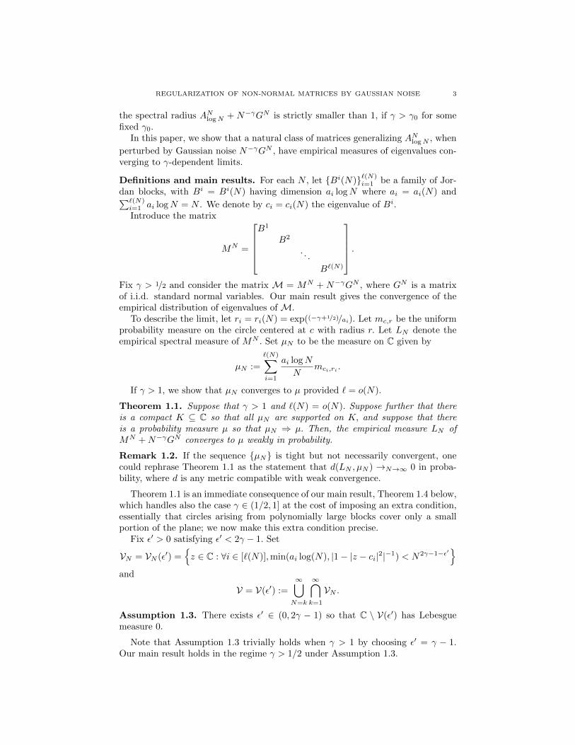
Figure 1. The eigenvalues of a deterministic 5000 × 5000 ma-trix perturbed by two different magnitudes of noise. The ma-trix consists of 5 types of blocks centered at −1, 0, 1,−0.5 −0.8i, and 0.5 − 0.8i. The sum of the dimensions of the blocks foreach type is roughly the same. Each individual block is of dimen-sion dlog 5000e = 9. Note the finite N effects.
Theorem 1.4. Suppose that γ > 1/2, `(N) = o(N) and Assumption 1.3 holds.Suppose further that there is a compact K ⊆ C so that all µN are supported onK, and suppose that there is a probability measure µ so that µN ⇒ µ. Then theempirical measure LN of MN +N−γGN converges to µ weakly in probability.
As mentioned before, Assumption 1.3 holds automatically when γ > 1, andtherefore Theorem 1.1 follow immediately from Theorem 1.4. An illustration of theγ-dependency in Theorem 1.4 is given in Figure 1.
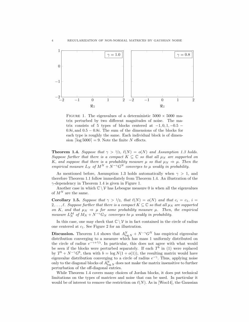
Another case in which C \ V has Lebesgue measure 0 is when all the eigenvaluesof MN are the same.
Corollary 1.5. Suppose that γ > 1/2, that `(N) = o(N) and that ci = c1, i =2, . . . , `. Suppose further that there is a compact K ⊆ C so that all µN are supportedon K, and that µN ⇒ µ for some probability measure µ. Then, the empiricalmeasure LMN of MN +N−γGN converges to µ weakly in probability.
In this case, one may check that C \ V is in fact contained in the circle of radiusone centered at c1. See Figure 2 for an illustration.
Discussion. Theorem 1.4 shows that ANlogN + N−γGN has empirical eigenvaluedistribution converging to a measure which has mass 1 uniformly distributed onthe circle of radius e−γ+1/2. In particular, this does not agree with what wouldbe seen if the blocks were perturbed separately. If each T b in (1) were replacedby T b + N−γGb, then with b = logN(1 + o(1)), the resulting matrix would haveeigenvalue distribution converging to a circle of radius e−γ . Thus, applying noiseonly to the diagonal blocks of ANlogN does not make the matrix insensitive to furtherperturbation of the off-diagonal entries.
While Theorem 1.4 covers many choices of Jordan blocks, it does put technicallimitations on the types of matrices and noise that can be used. In particular itwould be of interest to remove the restriction on `(N). As in [Woo14], the Gaussian
REGULARIZATION OF NON-NORMAL MATRICES BY GAUSSIAN NOISE 5
−0.5
0
0.5
y
−0.5
0
0.5
−0.5 0 0.5
−0.5
0
0.5
x
y
−0.5 0 0.5
−0.5
0
0.5
x
Figure 2. For various values of N, set MN to be the matrixwith all eigenvalues equal to 0 and approximately equal numberof blocks of size 0, 1, 2, . . . , dlogNe. From left-to-right and top-to-bottom, the eigenvalues of MN + N−γGN are given for γ = 3/4and N = 500, 1000, 2000, and 4000. The limiting density is givenby −C/r log r1
r ≤ e−1/4
for normalizing constant C.
assumption on the noise probably could also be weakened, though this requires abetter understanding of how small det(G+C) can be, where G is a matrix of i.i.d.elements and C is some arbitrary matrix (in particular, without a priori estimateson the norm of C); such control is not currently available for small singular valuesof G + C without putting some a-priori conditions on C, see e.g. [TV10] for thecase of minimal singular value.
Far beyond these possible extensions, it would be interesting to generalize The-orem 1.4 to cover matrices that are not in Jordan form, i.e. proving a theoremabout the noise perturbation of SNMN (SN )−1 for MN in Jordan form. This how-ever seems to require some constraints on the sequence SN so that they do notbecome progressively ill-conditioned going down the sequence.
Proof approach. The approach is based on the in-probability convergence ofthe logarithmic potential of LN to the logarithmic potential of the correspond-ing measure, which appears frequently in the study of non-normal random matri-ces (see [BC12]). For a compactly supported probability measure ρ on C, defineUρ(z) =
∫C log |z − x| dρ(x). Note the logarithmic potential of LN can also be ex-
pressed as ULN (z) = 1N log |det(M− zI)|, where I is the identity matrix.
To show the desired convergence of LN to µ, it suffices to show that:
a) There is a compact K ⊆ C so that for all ε > 0, Pr [LN (Kc) > ε]→ 0.
b) For almost every z ∈ C, ULN (z)P→ Uµ(z).
6 REGULARIZATION OF NON-NORMAL MATRICES BY GAUSSIAN NOISE
For a proof, see Theorem 2.8.3 of [Tao12]. The tightness condition a) is standard,and quickly follows from the assumed compact support of the collection µN.Thus, one needs to checks the convergence in b). Toward this end, we first discussthe convergence of UµN to Uµ.
Since µ is a probability measure, Uµ(z) ∈ Lploc for each 1 ≤ p <∞. In particular,Uµ(·) is finite almost everywhere. Together with the existence of the compact Kthat contains the support of the different µN , we also have the uniform integrabilityof UµN on compact subsets of C. Together with the weak convergence µN ⇒ µ, thisimplies that UµN → Uµ in Lploc. Passing to subsequences if necessary, we deducethe convergence of UµN (z) to Uµ(z) for Lebesgue almost every z. Thus, the proofof b), and therefore of Theorem 1.4, is reduced to showing
∀z ∈ V : |ULN (z)− UµN (z)| P→ 0.(2)
We obtain the convergence in (2) by showing upper and lower bounds on ULN (z).The upper bound is obtained through a careful expansion of the determinant ofM−zI = MN+N−γGN−zI as a linear combination of the minors of N−γGN . Theminors of GN are then bounded by a relatively crude union bound (see Lemma 3.2),and the sum is estimated by a leading order term analysis.
The upper bound argument works with significantly weaker assumptions thanTheorem 1.4. In particular Assumption 1.3 is not used at all. Furthermore, it shouldbe straightforward to weaken the assumptions on the noise to include entries whosedistributions are either non-Gaussian i.i.d., or Gaussian with non-trivial covariancematrix.
The lower bound, on the other hand, is more delicate. Here we first apply asequence of row and column permutations to the matrix to put it in the form
M− zI =
[A+G1 ∗∗ G2
],
(see (17)), where G1 and G2 are pure noise matrices and A is stable with respect toGaussian perturbation. This representation allows us to compute the determinantby the Schur complement formula, whose general form
det(M− zI) = det(A+G1) det(G2 − C),
where C is some matrix.As A is stable with respect to Gaussian perturbation, we use a second moment
computation to show that the determinant of A + G1 is a good approximation ofthe determinant of A. By showing that |det(G2 − C)| stochastically dominates|detG2|, we are able to obviate understanding C. In this step we crucially use theGaussian assumption on the matrix, and we believe this portion of the argumentis the largest obstruction to proving the theorem for more general noise models.
Assumption 1.3 is necessary for the second moment estimate. As can be seenfrom calculating the variance of det(I + zTN +N−γGN ) for various z with |z| < 1and 1/2 < γ ≤ 1, if z is very close 1 (going to 1 at some polynomial rate), the variancecan be made to grow to infinity, while the expectation is 1. This phenomenondisappears when γ > 1, for which reason Assumption 1.3 is vacuous for these γ.Thus for the purpose of showing det(A+G1) ≈ det(A), the second moment methodis an insufficient tool when 1/2 < γ ≤ 1. It is unclear whether Assumption 1.3 couldbe weakened or completely omitted by applying other methods of proof.
REGULARIZATION OF NON-NORMAL MATRICES BY GAUSSIAN NOISE 7
Organization. This paper is organized into 5 sections. In Section 2, we establishnotation that we use throughout the paper as well as many relevant calculationsand lemmata that we need for the upper and lower bounds. In Section 3, we showthe upper bound on the log potential, and in Section 4 we show the lower bound.In Section 5, we give the proof of Theorem 1.4.
2. Preliminaries
In this section we present notation and auxiliary lemmata that are used to sim-plify the rest of the paper. These are divided according to their general topic.Throughout the paper, whenever we state that a property holds with high proba-bility this is meant to say that the probability tends to 1 as N tends to infinity.
Log potential. For a natural number k, we let [k] := 1, 2, 3, . . . , k. To simplifyour calculations and definitions, we set
ν := γ − 1/2.
Also, we often omit the dependence of parameters on N.For each i ∈ [`], define
gi := (−ν)− ai log |z − ci|.This allows the log potential UµN (z) to be given by
(3)N
logNUµN (z) =
∑i:gi≤0
ai log |z − ci| −∑i:gi>0
ν.
Note that the expression is continuous in z.
Matrix decomposition. For an N × N matrix A, and X,Y ⊆ [N ] we writeA[X,Y ] for the submatrix of A which consists of the rows in X and the columns inY .
Our goal is to provide upper and lower bounds on 1N log |det(M−zI)| which are
arbitrarily close to UµN (z) for large N . In the process of obtaining both bounds,M− zI is decomposed into a sum of matrices A and B. In general, we may expandthe determinant of the sum of two N ×N matrices A and B as
(4) det(A+B) =∑
X,Y⊂[N ]|X|=|Y |
(−1)sgn(σX) sgn(σY ) det(A[X; Y ]) det(B[X;Y ]),
where X := [N ] \ X, Y := [N ] \ Y and σZ for Z ∈ X,Y is the permutation inSN which places all the elements of Z before all the elements of Z, but preservesthe order of elements within the two sets. In particular, observe that the notationA[X; Y ] denotes the submatrix of A given by deleting the rows inX and the columnsin Y .
In our application A will be an upper bi-diagonal block matrix with ` blocks,that is, a block matrix whose non-zero entries lie on the main diagonal and thefirst superdiagonal. For such a block matrix, Ai is used to denote the i-th block.Likewise, Xi, Yi are used to denote the rows and columns of Ai that are contained inX and Y respectively. This notation allows the decomposition of the determinantof a submatrix of a block matrix as a product of determinants of small matrices.Here and in the rest of our formulae we always assume the determinant of thematrix of size 0 to be one.
8 REGULARIZATION OF NON-NORMAL MATRICES BY GAUSSIAN NOISE
Lemma 2.1. Let A be an N × N block matrix with ` blocks, and let X,Y ⊂ [N ]be such that |X| = |Y |. We have
det(A[X;Y ]) =
∏`i=1 det(Ai[Xi;Yi]) ∀i ∈ [`] : |Xi| = |Yi|
0 otherwise.
Proof. We let k = |X| = |Y |. Suppose the second case holds. By permuting theorder of blocks, we may assume without loss of generality |X1| > |Y1|. Expandingthe determinant of U [X;Y ] by the Leibniz formula to get
det(A[X;Y ]) =∑σ∈Sk
sgn(σ)
k∏i=1
A[X;Y ]i,σ(i),
we observe that by the pigeonhole principle every σ ∈ Sk must satisfy σ(i) > |Y1|for some i ≤ |X1|. For this i we have A[X;Y ]i,σ(i) = 0, and therefore the entireproduct nullifies. In the first case where |Xi| = |Yi| for all i, it is straightforwardto check that the determinant is that of a block matrix, and thus it is the productof the block determinants.
Additionally, when A is an upper bi-diagonal block matrix, we can further sim-plify Lemma 2.1.
Lemma 2.2. Let A be an N × N block matrix with ` blocks, and let X,Y ⊂ [N ]be such that |X| = |Y |. If in addition A is upper bi-diagonal, then det(A[X;Y ]) isgiven by the product of its diagonal entries.
Proof. We let k = |X| = |Y | and write
X = x1 < x2 < . . . < xk and
Y = y1 < y2 < . . . < yk .Expand the determinant of A[X;Y ] by the Leibniz formula to get
det(A[X;Y ]) =∑σ∈Sk
sgn(σ)
k∏i=1
A[X;Y ]i,σ(i),
The claim is equivalent to showing that for all σ not equal to the identity,∏ki=1Axi,yσ(i) = 0. From bi-diagonality, if any yσ(i) /∈ xi, xi + 1, then Axi,yσ(i) is
0, and the claim is complete. Thus, we may restrict ourselves to yσ(i) ∈ xi, xi+ 1for all i ∈ [k]. Since xi and yi are strictly increasing, we deduce that σ(1) ≤ σ(2) ≤· · · ≤ σ(k). As σ is a permutation, this forces all these inequalities to be strictand hence σ is the identity. Thus only the identity permutation can possibly have∏ki=1Axi,σ(yi) 6= 0.
We conclude this part by presenting yet another simplification of the formula fordet(U [X; Y ]) when U is a single block of the form I + zTN .
Lemma 2.3. Let U = I + zTN . For X,Y ⊆ [N ] with |X| = |Y | = k, writeX = x1 < x2 < . . . < xk and Y = y1 < y2 < . . . < yk. Then
det(U [X; Y ]) =
k∏i=1
zxi−yi1 yi ≤ xi < yi+1,∀i, 1 ≤ i ≤ k ,
where we take yk+1 =∞.
REGULARIZATION OF NON-NORMAL MATRICES BY GAUSSIAN NOISE 9
Proof. Write X = w1 < w2 < . . . < wN−k and Y = z1 < z2 < . . . < zN−k . Us-ing Lemma 2.2 we observe that
(5) det(U [X; Y ]) =
N−k∏i=1
Uwi,zi .
Observe that by the bi-diagonal structure of U , this product nullifies unless
(6) zr ∈ wr, wr + 1 ∩ X.For i ∈ [k+ 1] write Ui = xi−1 + 1, xi−1 + 2, . . . , xi setting x0 = 0 and xk+1 = N .Since xi ∈ X we have by (6) that unless zr ∈ Ui for all r satisfying wr ∈ Ui, theproduct (5) nullifies. Since for all i ∈ [k] we have |r : wr ∈ Ui| = |Ui| − 1 and|r : wr ∈ Uk+1| = |Uk+1|, we conclude that each Ui with 1 ≤ i ≤ k containsexactly one element of Y , and the k + 1 block contains none of them. This impliesthat unless
y1 ≤ x1 y2 ≤ x2 · · · yk ≤ xk,the product (5) nullifies. The stated formula for the determinant now follows bynoting that for a given block Uj∏
i:xi∈Uj
Uxi,yi = zxj−yj .
Gaussian estimates. In this section, we present several lemmata involving esti-mates on the determinant of a Gaussian matrix. All the bounds in this sectionare based on the following identity in law for an N ×N matrix E of independentstandard Gaussians, see [Goo63],
|detE|2 L=N∏r=1
χ2r,
where χr are independent and have the distribution of the length of an r-dimensionalstandard Gaussian vector. For t > − r2 , we have the following moment formula forthe χr variable:
(7) Eχ2tr = 2t
Γ( r2 + t)
Γ( r2 ).
Lemma 2.4. Let E be an k × k matrix of independent standard Gaussians. Forany δ > 0, the following holds,
Pr[det |E| ≥ (k!)
1/2+δ]≤ exp
(−bkδc2(log(k/2e2)
)Proof. For natural numbers r and t, the χr moment formula (7) simplifies to
Eχ2tr = r(r + 2)(r + 4) · · · (r + 2t− 2).
Thus for some natural t, the moment of the determinant can be given by
E|detE|2t =
k∏r=1
t−1∏i=0
(r + 2i) ≤ k!(k + 2)!(k + 4)! · · · (k + 2t− 2)!.
For t ≤ N, this can be bounded by
E|detE|2t ≤ (k!)t(2k)t2
.
10 REGULARIZATION OF NON-NORMAL MATRICES BY GAUSSIAN NOISE
By Markov’s inequality, we therefore have that
Pr[det |E| ≥ (k!)
1/2+δ]≤ (k!)t(2k)t
2
(k!)t+2δ
for any integer t ≤ k. Using that k! ≥ kke−k, we get that
Pr[det |E| ≥ (k!)
1/2+δ]≤ exp
(t2 log(2k)− 2tδk log(k/e)
)= exp
(t2 log(2k)− tδk log(k
2/e2)
)for any integer t ≤ k. Taking t = bkδc, we get
Pr[det |E| ≥ (k!)
1/2+δ]≤ exp
(bkδc2 log(2k)− bkδcδk log(k
2/e2)
)≤ exp
(bkδc2 log(2e2/k)
).
Lemma 2.5. Let E be an N×N matrix of independent standard Gaussians. Thenthere are constants c1 > 0 and c2 > 0 so that
Pr[det |E| ≤
√N !e−c1N
]≤ 1
c2e−c2N .
Proof. We will use negative moments and Markov’s inequality to get the desiredbound. Fix an integer K > 0. Note that
FK :=
k∏r=1
χr
is absolutely continuous and has a bounded density. Thus, the probability thatFK < 2−N is exponentially small in N.
To prove the statement of the lemma, it therefore suffices consider LK :=∏Nr=K+1 χr. For this variable, we need to show that there are constants ci > 0
so that for N > K,
Pr[LK ≤
√N !e−c1N
]≤ 1
c2e−c2N .
Now by (7)
Eχ−2r =
1
(r − 2).
Thus for some K sufficiently large, we get that for all r > K,
Eχ−2r ≤
2
r.
Hence for this K,
EL−2K ≤ K!
2N
N !.
Applying Markov’s inequality we get
Pr[LK ≤
√N !2−N
]= Pr
[L−2K ≥
4N
N !
]≤ K!2−N ,
completing the proof.
REGULARIZATION OF NON-NORMAL MATRICES BY GAUSSIAN NOISE 11
3. Upper bound
This section is dedicated to the proof of the following proposition.
Proposition 3.1. For ` = o(N) and any z ∈ C, we have that for all δ > 0,
Pr [ULN (z) ≤ UµN (z)− δ]→ 0.
Let S denote the collection of blocks so that |z − ci| ≥ 1. Define U to be amodification of the matrixM− zI in which each column intersecting a block fromS is scaled by |z − ci|−1. This implies the following relationship:
(8) |det(M− zI)| = |det U|∏i∈S|z − ci|ai logN
Decompose U as a sum of M + G, where M = EU. This gives M the same blockstructure as M.
Write k = (ki)i∈[`] for an element of the hypercube 0, 1`. We define Πk as thesubset of (X,Y ), |X| = |Y | which satisfies:
(1) For each i ∈ [`], |Xi| = |Yi|.(2) For each i ∈ [`], |Xi| > 0 if and only if ki = 1.
Combining this together with Lemma 2.1 and (4) we have
det(U) =∑
k∈0,1`
∑(X,Y )∈Πk
(−1)s(X,Y ) det(M[X; Y ]) det(G[X;Y ]).
By taking absolute value and applying the triangle inequality, this implies
|det U| ≤∑
k∈0,1`
∑(X,Y )∈Πk
|det M[X; Y ] det G[X;Y ]|.(9)
Define the weight wk(z) by
(10) wk(z) :=∏
i∈[`]\S
|z − ci|(1−ki)ai logN .
By Lemma 2.2, for any X,Y ⊆ [N ] the minor |det M[X; Y ]| is given by the productof its diagonal entries. All entries of M are bounded by 1. For those (X,Y ) ∈ Πk,the diagonal entries of blocks for which ki = 0 can be bounded by |z − ci|. Hence,we get the bound
|det M[X; Y ]| ≤ wk(z) ≤ 1.
To complement this bound, we control the magnitude of det G[X;Y ] over allminors.
Lemma 3.2. For any fixed δ > 0, there is a constant C > 0 so that, with highprobability, for all X,Y ⊆ [N ] with |X| = |Y | = k we have
|det G[X;Y ]| ≤ C(k!)1/2+δ/logNN (−ν−1/2)ke(logN)C .
Proof. We apply a union bound over all choices (X,Y ) with |X| = |Y |. Let ΩNdenote the event that all elements of G are at most N−ν−1/2 logN in modulus;because the entries are standard Gaussian, Pr(ΩN ) → 1 as N → ∞. Thus, forchoices of (X,Y ) with |X| = k ≤ (logN)3, we have on ΩN that
|det G[X;Y ]| ≤ k!N (−ν−1/2)k(logN)k ≤ N (−ν−1/2)ke(logN)4
for all N large.
12 REGULARIZATION OF NON-NORMAL MATRICES BY GAUSSIAN NOISE
For (X,Y ) with |X| = |Y | = k > (logN)3, we apply Lemma 2.4 to get that
Pr[|det G[X;Y ]| ≥ N (−ν−1/2)k(k!)
1/2+δ/logN]≤ e−bkδ/logNc2 log(k/2e2).
Summing over all choices of (X,Y ), we have that
Pr[∃(X,Y ), |X| > (logN)3 : |det G[X;Y ]| ≥ N (−ν−1/2)|X|(|X|!)1/2+δ/logN
]≤
N∑k=d(logN)3e
(N
k
)2
e−bkδ/logNc2 log(k/2e2)
≤N∑
k=d(logN)3e
N2ke−ck4/3δ2 log(k) ≤ e−O((logN)4),
completing the proof.
In light of Lemma 3.2 and (10), it is possible to rewrite (9) as
|det U| ≤ Ce(logN)C∑
k∈0,1`wk(z)
∑(X,Y )∈Πk
(|X|!)1/2+δ/logNN (−ν−1/2)|X|
≤ Ce(logN)C∑
k∈0,1`wk(z)
(eδN−ν
)|k‖1 ∑(X,Y )∈Πk
(eδN−ν
)(|X|−‖k‖1).(11)
Next, we apply the following estimate, whose proof we postpone to the end ofthis section, to conclude the proof of Proposition 3.1.
Lemma 3.3. For any k ∈ 0, 1`,∑(X,Y )∈Πk
(eδN−ν
)(|X|−‖k‖1) ≤ e2eδ/2N1−ν/2.
Applying Lemma 3.3 to (11), we get
|det U| ≤ Ce(logN)Ce2eδ/2N1−ν/2 ∑k∈0,1`
wk(z)(eδN−ν
)‖k‖1.
By our assumption that ` = o(N) we may replace the sum by a maximum:
1
Nlog |det U| ≤ o(1) + max
k∈0,1`
log(wk(z)
(eδN−ν
)‖k‖1)N
= o(1) +logN
N
∑i∈[`]\S
max(ai log |z − ci|,−ν + δ/logN),(12)
where the last equality follows from (10). We observe that
max(ai log |z − ci|,−ν + δ/logN) =
ai log |z − ci| if gi ≤ −δ/logN and
−ν + δ/logN if gi > −δ/logN.
Writing J := i ∈ [`] : gi ≤ −δ/logN, Translating (12) into:
(13)1
Nlog |det U| ≤ o(1) +
logN
N
∑i∈J\S
ai log |z − ci|+logN
N
∑i∈[`]\(J∪S)
(−ν + δ/logN) .
REGULARIZATION OF NON-NORMAL MATRICES BY GAUSSIAN NOISE 13
Thus using (8) and (13), we have shown that with probability going to 1, for δ < ν,we have
1
Nlog |detM− zI| = log |det U|
N+
logN
N
∑i∈S
ai log |z − ci|
= o(1) +logN
N
∑i∈J
ai log |z − ci|+logN
N
∑i∈[`]\J
(−ν + δ/logN)
≤ o(1) +logN
N
∑i∈J
ai log |z − ci|+logN
N
∑i∈[`]\J
−ν.(14)
Where the second equality uses the fact that gi < −ν < −δ for i ∈ S, and theinequality uses the assumption that ` = o(N).
Rewriting (3), we have the following bound on UµN (z) :
UµN (z) =logN
N
∑i:gi<0
ai log |z − ci| −logN
N
∑i:gi≥0
ν.
The bound given in (14) differs only in that some terms for which −δ/logN < gi ≤ 0have been moved from the second sum to the first. Thus (14) can be rewritten as
ULN (z) ≤ UµN (z) + o(1) +logN
N
∑i∈[`]\Jgi≤0
−gi.
As [`] = o(N) and gi > −δ/logN for all i ∈ [`] \ J , we get
ULN (z) ≤ UµN (z) + o(1),
as required.
Proof of Lemma 3.3. Let m = (mi)i∈[`] denote an element of the set
T := [a1 logN ]× [a2 logN ]× · · · × [a` logN ],
and let Tm,k ⊂ Πk denote the collection of pairs (X,Y ) so that mi = |Xi| = |Yi|.Note that this forces mi = 0 for all those i ∈ [`] so that ki = 0.
The cardinality of Tm,k is given by
|Tm,k| =∏i:ki=1
(ai logN
mi
)2
.
14 REGULARIZATION OF NON-NORMAL MATRICES BY GAUSSIAN NOISE
We may then use this to obtain the bound,
∑(X,Y )∈Πk
(eδN−ν
)(|I|−‖k‖1)=
N∑j=‖k‖1
∑m∈T‖m‖1=j
|Tm,k|(eδN−ν
)(j−‖k‖1)
=
N∑j=‖k‖1
∑m∈T‖m‖1=j
∏i:ki=1
(ai logN
mi
)2 (eδN−ν
)(mi−1)
=∏i:ki=1
[ai logN∑mi=1
(ai logN
mi
)2 (eδN−ν
)(mi−1)]
≤∏i:ki=1
[ai logN∑mi=0
(ai logN
mi
)2 (eδN−ν
)mi].
As∑ai logNmi=0
(ai logNmi
)2 (eδN−ν
)mi> 1 for all i ∈ [`] we can complete the product
to get:
∑(X,Y )∈Πk
(eδN−ν
)(|I|−‖k‖1) ≤∏i=1
[ai logN∑mi=0
(ai logN
mi
)2 (eδN−ν
)mi].(15)
For any q > 0 and any t ∈ N, define the polynomial
Pt(q) =
t∑m=0
(t
m
)2
qm.
Thus, in terms of (15), we have
(16)∑
(I,J)∈Πk
(eδN−ν
)(|I|−‖k‖1) ≤∏i=1
Pai logN
(eδN−ν
).
We now bound Pt(q), by comparing with Taylor series:
Pt(q) =
t∑m=0
(t
m
)2
qm ≤t∑
m=0
t2m
(m!)2qm ≤
t∑m=0
t2m
(2m)!qm(
2m
m
)
≤∞∑m=0
t2m
(2m)!qm22m ≤
∞∑m=0
(2t√q)m
m!= e2t
√q.
Combining this bound with (16), we get that
∑(I,J)∈Πk
(eδN−ν
)(|I|−‖k‖1) ≤ exp
(2(eδN−ν
)1/2∑i=1
ai logN
).
As∑`i=1 ai logN = N, the proof is complete.
REGULARIZATION OF NON-NORMAL MATRICES BY GAUSSIAN NOISE 15
4. Lower bound
This section is dedicated to the proof of the following proposition.
Proposition 4.1. For z ∈ VN , ` = o(N) we have that for all δ > 0,
limN→∞
Pr [ULN (z) ≤ UµN (z)− δ] = 0.
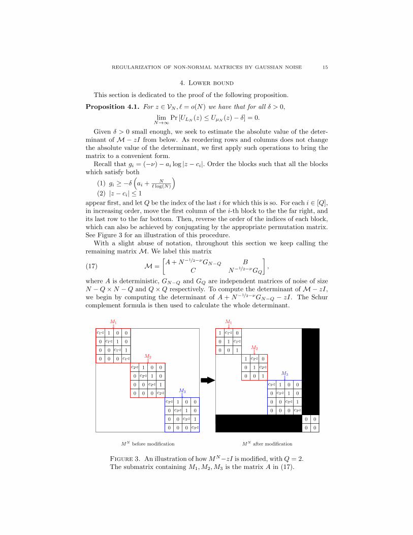
Given δ > 0 small enough, we seek to estimate the absolute value of the deter-minant of M− zI from below. As reordering rows and columns does not changethe absolute value of the determinant, we first apply such operations to bring thematrix to a convenient form.
Recall that gi = (−ν)− ai log |z − ci|. Order the blocks such that all the blockswhich satisfy both
(1) gi ≥ −δ(ai + N
` log(N)
)(2) |z − ci| ≤ 1
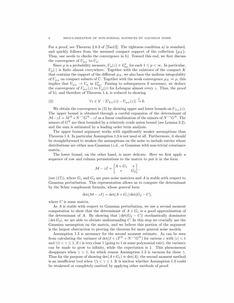
appear first, and let Q be the index of the last i for which this is so. For each i ∈ [Q],in increasing order, move the first column of the i-th block to the the far right, andits last row to the far bottom. Then, reverse the order of the indices of each block,which can also be achieved by conjugating by the appropriate permutation matrix.See Figure 3 for an illustration of this procedure.
With a slight abuse of notation, throughout this section we keep calling theremaining matrix M. We label this matrix
(17) M =
[A+N−1/2−νGN−Q B
C N−1/2−νGQ
],
where A is deterministic, GN−Q and GQ are independent matrices of noise of sizeN −Q×N −Q and Q×Q respectively. To compute the determinant of M− zI,we begin by computing the determinant of A + N−1/2−νGN−Q − zI. The Schurcomplement formula is then used to calculate the whole determinant.
c1-z 1 0 0
0 c1-z 1 0
0 0 c1-z 1
0 0 0 c1-z
c2-z 1 0 0
0 c2-z 1 0
0 0 c2-z 1
0 0 0 c2-z
c3-z 1 0 0
0 c3-z 1 0
0 0 c3-z 1
0 0 0 c3-z
MN before modification
M1
M2
M3
1 c1-z 0 0
0 1 c1-z 0
0 0 1 c1-z
1 c2-z 0 0
0 1 c2-z 0
0 0 1 c2-z
c3-z 1 0 0
0 c3-z 1 0
0 0 c3-z 1
0 0 0 c3-z
c1-z 0 0 0 0
c2-z 0 0 0 0
MN after modification
M1
M2
M3
Figure 3. An illustration of howMN−zI is modified, withQ = 2.The submatrix containing M1,M2,M3 is the matrix A in (17).
16 REGULARIZATION OF NON-NORMAL MATRICES BY GAUSSIAN NOISE
Write M, and G for the matrices A− zI and N−1/2−νGN−Q, denoting the i-thblock of M by Mi. As the determinant of L = M + G will be bounded using thesecond moment method, we begin by calculating Edet(L). Applying (4) to M andG implies:
(18) det(L) =∑
X,Y⊂[N−Q]|X|=|Y |
(−1)s(X,Y ) det(M[X; Y ]) det(G[X;Y ]).
For any X or Y 6= ∅, we have that Edet(G[X;Y ]) = 0. Thus, by the linearity ofexpectation, may deduce that
Edet(L) =∑
X,Y⊂[N−Q]|X|=|Y |
(−1)s(X,Y ) det(M[X; Y ])Edet(G[X;Y ])
= Edet(M)
=∏i/∈[Q]
(z − ci)ai logN .
Given that Edet(L) = Edet(M), the following claim would allow us to applyChebyshev’s inequality and prove Proposition 4.1.
Lemma 4.2. Given ` = o(N), for z ∈ VN , we have that there is a C = C(ν) > 0so that for all δ > 0 there is an N0 = N0(ν, δ) so that
Var det(L)/|det(M)|2 < C · δ
for N ≥ N0.
In the proof of Lemma 4.2 we shall make use of the following bound whose proofwe give after the proof of Lemma 4.2.
Lemma 4.3. For z ∈ VN and 1 > δ > 0, there is an N0 depending on ν, z and δ,so that for any i ∈ [`] and any Xi ⊆ [dim Mi],∑
|Yi|=|Xi|
|det(Mi[Xi; Yi])|2N−2ν|Xi| < |det(Mi)|2δ|Xi|
for all N ≥ N0.
Proof of Lemma 4.2. For any Xi, Yi ⊆ [N −Q], i = 1, 2 define
K(X0, Y0, X1, Y1)
= Cov(det(M[X0; Y0]) det(G[X0;Y0]),det(M[X1; Y1]) det(G[X1;Y1])).
Using (18), we reformulate the above as
Var det(L) =∑
Xi,Yi⊂[N−Q]|Xi|=|Yi|i=1,2
(−1)s(X0,Y0)+s(X1,Y1)K(X0, Y0, X1, Y1).(19)
REGULARIZATION OF NON-NORMAL MATRICES BY GAUSSIAN NOISE 17
Observe that if either X0 6= X1 or Y0 6= Y1, then K(X0, Y0, X1, Y1) = 0. Using this(19) reduces to
Var det(L) =∑
X,Y⊂[N−Q]|X|=|Y |
|det(M[X; Y ])|2 Var(det(G[X;Y ]))
=∑
X,Y⊂[N−Q]|X|=|Y |>0
|det(M[X; Y ])|2N−2(ν+1/2)|X|(|X|!)
Recall that Xi are the rows of X which intersect the block Mi and Yi are thecolumns of X which intersect the block Mi. This allows further development of(19) into
Var det(L) =∑
X⊂[N−Q]|X|>0
N−|X|(|X|!)∏i=1
∑|Yi|=|Xi|
|det(Mi[Xi; Yi])|2N−2ν|Xi|
=
N−Q∑k=1
N−kk!∑
X⊂[N−Q]|X|=k
∏i=1
∑|Yi|=|Xi|
|det(Mi[Xi; Yi])|2N−2ν|Xi|
≤N−Q∑k=1
maxX⊂[N−Q]|X|=k
∏i=1
∑|Yi|=|Xi|
|det(Mi[Xi; Yi])|2N−2ν|Xi|.(20)
Combining (20) with Lemma 4.3, we have
Var det(L) ≤N−Q∑k=1
maxX⊂[N−Q]|X|=k
∏i=1
∑|Yi|=|Xi|
|det(Mi[Xi; Yi])|2N−2ν|Xi|
≤N−Q∑k=1
maxX⊂[N−Q]|X|=k
∏i=1
|det(Mi)|2δ|Xi|
≤ |det(M)|2N−Q∑k=1
δk ≤ |det(M)|2 δ
1− δ .
We now turn to proving Lemma 4.3.
Proof of Lemma 4.3. We divide the proof into three cases, according to the type ofblock Mi. Define a partition of [`] = S1 ∪ S2 ∪ S3 by
S1 :=
i : gi ≥ −δ
(ai +
N
` logN
), |z − ci| ≤ 1
,
S2 :=
i : gi < −δ
(ai +
N
` logN
), |z − ci| ≤ 1
,
S3 := i : |z − ci| > 1 .Note that S1 = [Q].
18 REGULARIZATION OF NON-NORMAL MATRICES BY GAUSSIAN NOISE
Set k = |Xi|. Let Xi = x1, x2, . . . , xk , with x1 < x2 < · · · < xk. By virtue ofLemma 2.3, the only choices of Yi = y1, y2, . . . yk with y1 < y2 < · · · < yk whichwe need to consider are those which satisfy
x1 ≤ y1 < x2 ≤ y2 < · · · < xk ≤ yk.The case i ∈ S1: For i ∈ S1, we have that Mi has 1 on the diagonal and ci on the
superdiagonal. Thus, we may write
Ti :=∑
|Yi|=|Xi|
|det(Mi[Xi; Yi])|2 =
k∏j=1
xj+1−xj−1∑r=0
|z − ci|2r,
where we take xk+1 = dim Mi ≤ ai logN. This we may control either by boundingeach element by 1 or by bounding the truncated geometric series by the entiregeometric series, which implies
T1/ki ≤ min
ai logN,
1
1− |z − ci|2≤ N2ν−ε′ ,
where the rightmost inequality follows from the fact that z ∈ VN .The case i ∈ S3: This is nearly identical to the case i ∈ S1, and so we show it
first. For i ∈ S3, it is now the case that Mi has ci− z on the diagonal and 1 on thesuperdiagonal. Pulling out a factor of ci− z, we essentially reduce the determinantto the previous case, i.e.
Ti = |z − ci|2|Xi|∑
|Yi|=|Xi|
|det((z − ci)−1Mi[Xi; Yi])|2
= |z − ci|2|Xi|k∏j=1
xj+1−xj−1∑r=0
|z − ci|−2r
= |z − ci|2(ai logN−k)k∏j=1
xj+1−xj−1∑r=0
|z − ci|−2r
≤ |z − ci|2(ai logN−k)
[ai logN−1∑r=0
|z − ci|−2r
]k.(21)
Thus, on the one hand, we may bound the sum by bounding each term by 1, or wemay bound by a geometric series. In the first case we get
Ti≤|z−ci|2(ai logN−k)|ai logN |k≤|z−ci|2ai logN |ai logN |k= |det(Mi)|2|ai logN |k.In the second case we get
Ti ≤ |z − ci|2(ai logN−k)
[1
1− |z − ci|−2
]k= |det(Mi)|2
[1
|z − ci|2 − 1
]k.
Thus as z ∈ VN , it follows that
Ti ≤ |det(Mi)|2N (2ν−ε′)k.
The case i ∈ S2: As in the previous case, for i ∈ S2, the blocks Mi have ci − zon the diagonal and 1 on the superdiagonal. From Lemma 2.2, we have that|det(Mi[Xi; Yi])|2 ≤ 1, and hence
(22) Ti ≤ (ai logN)k.
REGULARIZATION OF NON-NORMAL MATRICES BY GAUSSIAN NOISE 19
Note that the condition that gi < −δai and |z − ci| ≤ 1 imposes a lower boundon the size of ai, namely
−δai > gi = −ν − ai log |z − ci| > −νand hence ai < ν/δ.
Let ξδ <∞ be the solution of δξδ = supx≥0 xe−2δx. We get that
ai logN ≤ δξδ · e2δai logN
As ` = o(N), there is an N1 = N1(δ) sufficiently large so that ξδ ≤ e2δN/` for allN ≥ N1. Hence, for all N ≥ max(N0, N1),(23)
ai logN ≤ δe2δai logN+2δN/` ≤ δe−2gi logN = δN2ν |z − ci|2ai logN = δN2ν |det Mi|2.Combining (22) and (23), it follows that
Ti ≤ (ai logN)k ≤ δkN2νk|det Mi|2k ≤ δkN2νk|det Mi|2
for all N sufficiently large.
Having controlled the determinant of A + N−1/2−νGN−Q, it remains to showthat the determinant of M− zI is not too small. Our proof rests on the followingstochastic domination lemma.
Lemma 4.4. Suppose that E is a Q×Q standard Gaussian matrix. Then for anyQ×Q matrix M independent of E and all t ≥ 0,
Pr [|det(E +M)| ≤ t] ≤ Pr [|detE| ≤ t] .Proof. The proof rests on the parallelpiped formula for the modulus of a determi-nant. For any square matrix M ′, let Sj(M
′) be the span of the first j columns.Then we have the following identity
|det(E +M)|2 =
Q∏j=1
∣∣∣proj(Sj−1(E+M))⊥ ((E +M)j)∣∣∣2 ,
where (E+M)j denotes the j-th column of E+M. By virtue of absolute continuitywith lebesuge measure, we have that each Sj(E+M) is almost surely j-dimensional.Conditioned on columns 1, 2, . . . , j and choosing an orthonormal basis for Sj−1(E+M)⊥, the projection proj(Sj−1(E+M))⊥ ((E +M)j) has the law of an uncentered
(Q − j + 1)-dimensional standard Gaussian vector. The norm of an uncenteredstandard Gaussian vector stochastically dominates the norm of a centered standardGaussian vector, and hence we have the relation
Pr
[∣∣∣proj(Sj−1(E+M))⊥ ((E +M)j)∣∣∣2 ≤ t ∣∣ σ(Sj−1(E +M))
]≤ Pr
[∣∣∣proj(Sj−1(E))⊥ ((E)j)∣∣∣2 ≤ t ∣∣ σ(Sj−1(E))
].
Hence, applying this relation iteratively, we get the desired result that
Pr[|det(E +M)|2 ≤ t
]≤ Pr
[|detE|2 ≤ t
].
20 REGULARIZATION OF NON-NORMAL MATRICES BY GAUSSIAN NOISE
With this result in hand, we finally prove to lower bound proposition using theSchur complement formula and Chebyshev’s inequality.
Proof of Proposition 4.1. Recall that
ULN (z) =1
Nlog |det(M− zI)|.
We will apply the Schur complement formula to compute this determinant, using theblock structure from (17). For δ > 0 sufficiently small, Lemma 4.2 and Chebyshev’sinequality imply that
|det(A+N−ν−1/2GN−Q − zI)| ≥ 1/2|det(M)|
with probability going to 1.As a corollary, the corner submatrixA+N−ν−1/2GN−Q−zI is invertible with high probability. Hence, we may apply the Schur complementformula to write
det(M− zI) = det(A+N−ν−1/2GN−Q − zI) det(N−ν−
1/2GQ − Z),
with Z someQ×Qmatrix independent ofGQ. Applying Lemma 4.4 and Lemma 2.5,we have that
|det(N−ν−1/2GQ − Z)| ≥ N (−ν−1/2)Q(Q!)1/2e−cQ
with high probabilty.By our assumption that ` = o(N), we get
ULN (z) ≥ 1
Nlog |det(M)| − (ν + 1/2)Q
logN
N+
1
2
Q(logQ)
N− o(1)
=1
Nlog |det(M)| − νQ logN
N+
1
2
Q(logQ− logN)
N− o(1)
=1
Nlog |det(M)| − νQ logN
N− o(1)
As det(M) is given by the product of its diagonal, we get
ULN (z) ≥ logN
N
∑i>Q
ai log |z − ci| −logN
N
∑i∈[Q]
ν − o(1).(24)
Recall that we wish to bound ULN (z) below by UµN (z), which is given by (3):
UµN (z) =logN
N
∑i:gi<0
ai log |z − ci| −logN
N
∑i:gi≥0
ν.
Observing that i ∈ [Q] implies gi < 0 we get
ULN (z)− UµN (z) =logN
N
∑i/∈[Q],gi<0
ai log |z − ci| −logN
N
∑i/∈[Q],gi<0
ν − o(1)
=logN
N
∑i/∈[Q],gi<0
gi + o(1)
<logN
N
∑i/∈[Q],gi<0
δN
` logN+ o(1)
< δ + o(1),
REGULARIZATION OF NON-NORMAL MATRICES BY GAUSSIAN NOISE 21
with the o(1) errors going to 0 at some absolute rate. Thus, we have that for allfixed δ, ULN (z) ≥ UµN (z)− δ with probability going to 1 as N →∞.
5. Proof of Theorem 1.4
From Propositions 3.1 and 4.1, and the assumption that µN ⇒ µ, we have that
for almost every z ∈ C, ULN (z)P→ Uµ(z). It follows from Theorem 2.8.3 of [Tao12]
that LN converges to µ vaguely in probability, i.e. for all compactly supportedcontinuous functions φ : C→ R,∫
Cφ(x)dLN (x)
P→∫Cφ(x)dµ(x).
To additionally conclude that the convergence holds in the weak topology, it
suffices to show that there is a compact K1 ⊆ C so that LN (Kc1)
P→ 0. Note thatas we assume there is a compact K ⊆ C so that µN is supported on K, it followsthere is an C sufficiently large so that all ci = ci(N) where 1 ≤ i ≤ ` = `(N) andN runs over N are bounded in modulus by C. Hence,
‖M‖op ≤ ‖MN +N−ν−1/2GN‖op
≤ ‖MN‖op + ‖N−ν−1/2GN‖op ≤ 1 + C + ‖N−ν−1/2GN‖op.
It is easily checked that ‖GN‖op ≤ C ′√N with high probability, for some sufficiently
large C ′. (In fact, taking C = 1 + δ with arbitrary δ > 0 suffices.) Since ν > 0, theexistence of the claimed K1 follows and completes the proof of the theorem.
Acknowledgements.
We thank Naomi Feldheim, Mark Rudelson and Misha Sodin for useful sugges-tions.
References
[AGZ10] G. W. Anderson, A. Guionnet and O. Zeitouni, An Introduction to Random Matrices,Cambridge Univ. Press, 2010.
[BC12] C. Bordenave and D. Chafaı, Around the circular law, Probab. Surv. 9, 1–89 (2012).[Bha97] R. Bhatia, Matrix analysis, Springer, 1997.
[Goo63] N. R. Goodman, Distribution of the determinant of a complex Wishart distributedmatrix, Annals of Mathematical Statistics 34, 178–180 (1963).
[GWZ14] A. Guionnet, P. M. Wood and O. Zeitouni, Convergence of the spectral measure of
non-normal matrices, Proc. Amer. Math. Soc. 142(2), 667–679 (2014).
[Sni02] P. Sniady, Random regularization of Brown spectral measure, J. Funct. Anal. 193(2),
291–313 (2002).[Sun96] J.-G. Sun, On the variation of the spectrum of a normal matrix, Linear Algebra and
its Applications 246(0), 215 – 223 (1996).
[Tao12] T. Tao, Topics in random matrix theory, volume 132 of Graduate Studies in Mathe-matics, American Mathematical Society, Providence, RI, 2012.
[TE05] L. N. Trefethen and M. Embree, Spectra and pseudospectra: the behavior of nonnormal
matrices and operators, Princeton University Press, 2005.[TV10] T. Tao and V. Vu, Smooth analysis of the condition number and the least singular
value, Math. Comp. 79(272), 2333–2352 (2010).[Woo14] P. Wood, Universality of the ESD for a fixed matrix plus small random noise: a stability
approach, (2014).