ERASMUS UNIVERSITY ROTTERDAM

ERASMUS SCHOOL OF ECONOMICS

MSc Economics & Business

Master Specialization Financial Economics

A Macroeconomic Perspective on Asset Holders’ Risk Aversion

Abstract:

The unequal distribution of wealth and income causes only a relatively small number of people in

developed countries to own stocks. As a result, consumption by stockholders differs from that of non-

stockholders. This has been demonstrated by a number of studies, which have all made use of consumer

survey data. These data are scarce though and the approximation of stockholders’ and non-stockholders’

consumption by long time series data could greatly enhance our understanding of asset markets. This

paper is the first attempt to show empirically that the difference between consumption by stockholders

and by non-stockholders can also be illustrated with macroeconomic data from national accounts. Data

from seven different economies will show that stockholders’ consumption growth tends to be more

volatile than that of non-stockholders’ and that there is a stronger correlation to the excess returns on

stock markets. This partly explains why equity premiums in developed economies have been so high,

although it cannot resolve the equity premium puzzle completely.

Finish data: January 2010

Thesis coordinator: Prof. Dr. C. de Vries

Student: Peter de Bruin

Nr: 161455

Mail: ppdebruin@hotmail.com

Tel: 0618889055

1

Table of Contents:

Foreword: Hats off to my mother! 3

Section 1: Introduction: 3

Section 2: What is the equity premium puzzle about? 3

2.1 A risk premium? 3

2.2 Introduction to the puzzles 3

2.2.1 The equity premium puzzle 3

2.2.2 The risk free rate puzzle 3

Section 3: Literature review 3

3.1 Introduction 3

3.2 Three common assumptions and the equity premium puzzle 3

3.3 Different utility functions 3

3.3.1 Generalized expected utility 3

3.3.2 Habit formation 3

3.3.3 Catching up with the Joneses (relative consumption) 3

3.4 Incomplete markets and trading costs 3

3.4.1 Idiosyncratic income risk, which cannot be insured 3

3.4.2 Trading and Transaction costs 3

3.5 Other explanations 3

3.5.1 Transaction services return 3

3.5.2 Survivorship bias 3

3.5.3 Disaster States 3

3.5.4 Myopic loss aversion an the equity premium puzzle 3

3.6 Market segmentation 3

3.6.1 Unequal distribution of income and wealth 3

3.6.2 Market segmentation 3

Section 4: Explanation of the model and methodology 3

4.1 Introduction 3

4.2 The model 3

4.3 Data and methodology 3

4.3.1 Consumption of non-stockholders 3

4.3.2 Consumption of stockholders 3

4.3.3 Year-on-year changes instead of quarterly changes 3

4.3.4 Consumption is a flow variable 3

4.3.5 The equity premium is calculated with stock variables 3

Section 5: Examining the characteristics of stockholders’ consumption 3

2

Section 6: Conclusion and discussion 3

6.1 Conclusion 3

6.2 Other issues 3

6.2.1 Globalization 3

6.2.2 Accounting for other assets than equity 3

6.2.3 A cross-border comparison of stockholders’ risk aversion 3

Appendix A: The coefficient of risk aversion and the elasticity of intertemporal substitution 3

Appendix B: Labor Income data in the national accounts 3

Appendix C: Average effective tax rates on labor income 3

Appendix D: EViews programs 3

Websites 3

References 3

3

Foreword: Hats off to my mother!

Looking back on my time as a student one person stands out. My mother! How hard must it have been for

her, being severely ill herself, to cope with her son’s poor health. Yet, a phone call never remained

unanswered, and any issue, no matter how difficult or painful, could always be resolved. I can honestly

say that without her support, I don’t think I would have come as far as I have come today.

I should start by making an apology, though. My desire to study and get healthy against a

background of difficulties often led me to believe that I should have been the first to get attention. Allow

me to explain this as – a soon to be – economist. Whenever an equilibrium between two persons is Pareto

optimal, one can only benefit by making the other lose. Often this was precisely what happened. My

needs to be helped simply came at my mother’s expense. This was of course not right, and mama I am

sorry. Please, let anybody who reads this remind me of these words, when as my ambitions take center

stage again, I forget what is really important in life.

I should also not forget to thank my father. Our relationship is different. We share the same

intellectual curiosity. The writer Samuel Johnson could not have said it more clearly: “Knowledge always

desires increase, it is like fire, which must first be kindled by some external agent, but which afterwards

will propagate itself.” I still vividly remember us standing in front of the Eiffel tower in Paris a couple of

years ago. After having just finished a conversation about the French revolution, our attention shifted to

how the forces of gravity found there way to the ground. I still cannot help but smile when I think of my

father getting excited about how the rivets were shot through the steel of this magnificent structure. Over

time, I learned that his more problem-solving approach towards life has been his way to show affection

and love.

The following word of thanks perhaps sounds strange. But I would sincerely like to thank the

person, who hit me when as a teenager I was driving my motorcycle to get to school. Although we never

met, that moment of collision was an important moment, perhaps the most important moment in my life.

There is a Buddhist saying: “being happy is seeing right” and that is precisely what all those years of

illness after this accident taught me. I learned that “seeing right” in essence means trusting your own heart

and letting your feelings guide you through life. Consequently, the decade of illness made me a unique

person, a fact which I have come to appreciate more and more. My accident also taught me that life is

short and time precious. In a way this is a good thing. When the supply of life becomes shorter, it simply

makes us realize that the price of life is high. A finite life, which is lived according to this belief, at least

in my opinion, would be worth more than an infinite one (if this were to exist, of course).

Besides my parents and the person that ran me over, I would also like to take this opportunity to

thank student-dean Bernard den Boogert. On numerous occasions he helped me and I always had the

feeling that his attempts to assist me came “straight from the heart”. Frankly, I think it is great to have

4

people working at a university, which is characterized by its harsh business climate, who feel the urgency

to help the less gifted and ill.

I would like to finish this foreword by thanking Professor Casper de Vries. With hindsight, his

invitation to become student-assistant functioned as a catalyst in my development as an economist.

Furthermore, not only did he provide the idea behind this thesis, but he also said that he wanted to assist

me in writing it, even though circumstances have delayed this project by almost three years.

5

Section 1: Introduction

Stock returns across countries typically have an average real rate of return of more than 7 per cent. Short

term government debt, at the same time, rarely delivers an annual real yield that exceeds 3 percent. Why

has the real rate of return on stocks been significantly higher than the real rate of return on government

bonds? One answer to this question could be that stocks are considered to be more volatile, and hence

more risky. Investors therefore require an additional premium for holding stocks in preference to bonds,

i.e. the equity premium.

However, in 1985 Mehra and Prescott presented the economic profession a teaser. The historical

US equity premium has been of an order of magnitude larger than can be explained by a standard general

equilibrium asset pricing model, calibrated with plausible parameters. This has lead to the equity

premium puzzle. In essence, aggregate consumption growth does not co-vary enough with stock returns

to justify the risk premium observed for stocks. This leaves no other explanation for large returns than

implausibly high levels of risk aversion. Or to put it another way, the fact that stock prices change

randomly without affecting consumption growth very much, in no way represents true risk, and a large

equity premium is therefore not warranted.

Moreover, Weil (1989) showed that the data possesses another anomaly. If people are indeed

highly risk averse, they desire consumption to be consistent not only in terms of state, but also over time

(they dislike growth in consumption). Given that consumption, on average, increases steadily, individuals

must be inclined to borrow in order to reduce the difference between future and current consumption

expenditures. This leads to the risk-free rate puzzle. In asset pricing models, the reduced demand for

bonds causes the interest rate to be counterfactually high.

Although several contributions have been made that have deepened our understanding, both

puzzles seem to have been very difficult to solve. Various essential features of Mehra and Prescott’s

model have been amended to compensate for its poor performance. They include, among others,

alternative preference structures and different assumptions e.g. Epstein and Zin (1991), Constantinides

(1990), Abel (1990), Cambell and Cochrane (1995), Bernatzi and Thaler (1995). Reitz (1988) tries to

enhance the model, by taking into account the possibility of a disastrous but rare event. Brown et al

(1995) argue that the ex-post measured returns reflect the fact that only successful stock-exchanges

survive over time. As a result, the equity premium seen in reality should be a sub-set of a – largely

unobservable – sample, and consequently paints too positive a picture about true returns on stocks.

Heaton and Lucas (1995, 1996), Constantinides and Duffie (1995) turn their attention to the

incompleteness of markets, – i.e. the disability to create a contingent claim for every state of the world –

as a possible solution for the equity premium puzzle, while, Aiyergari and Gertler (1991), Aiyergari

(1993), Constantinides et al (2002) show that market imperfections could be a possible explanation for

the poor results obtained from the model.

6

A different but interesting route has been taken by Mankiw and Zeldes (1991). The unequal

distribution of wealth and income causes only a small percentage of the population to own stocks. As a

result, consumption by stockholders and non-stockholders is likely to differ. This suggests that market

segmentation may be possible. There is no a priori reason to expect someone who does not own an asset,

to adjust his or her consumption stream in response to anticipated changes in that asset’s price. Hence,

households that do not hold stocks are not likely to satisfy the first order condition that underlies the asset

pricing model in Mehra and Prescott’s work. The fact that characteristics of stockholders’ consumption

are likely to differ from those of non-stockholders implies that the modeled relationship between

aggregate consumption growth and stock returns is not likely to be accurate. Consequently, the standard

method of how the model is generally tested should be altered. When making inferences about the level

of risk aversion one should focus solely on the consumption growth of stockholders. Indeed, Mankiw and

Zeldes show that in the US stockholders’ consumption growth co-varies appreciably more with stock

returns than that of non-stockholders’. Their use of survey data, however, leaves serious room for

improvement, leading them to conclude their article with the question of “whether it might be possible to

approximate the consumption of stockholders using data that are available as a time series”.

This paper is the first attempt to show empirically that macroeconomic data is also a valid

instrument for representing the consumption of stockholders. Although this requires fairly rigid

assumptions, the issue of data availability disappears. A second advantage of macroeconomic data is that

results can be compared between different economies, making eventual conclusions more robust.

For seven developed economies, we construct a model with two groups of consumers. The first

group, which consists of the non-stockholders, only derives income from supplying labor to the labor

market and by assumption is restricted in its wealth resources. As a result, members of this group are

forced to consume their entire income. The second group, in contrast, consists of the stock-holders. These

consumers’ exclusive source of income is risk-based compensation they receive for providing capital to

the economy. Per definition, this group’s consumption is the total amount of consumption in the economy

minus the part consumed by the labor force (or differently, total consumption minus labor income).

Our results are encouraging. Growth in stockholders’ consumption is not only more volatile, but

also has a higher correlation with stock returns than non-stockholders’ consumption growth. This causes

the covariance between changes in stockholders’ consumer spending and the equity premium to be

significantly higher. In turn, the implied levels of risk aversion for stockholders are much more plausible

than for non-stockholders, although they cannot resolve the equity premium puzzle completely.

The remainder of this paper proceeds as follows. Section 2 specifies both the equity premium as

well as the risk-free rate puzzle. Section 3 briefly reviews the existing literature. Section 4 explains the

model and the use of data, while Section 5 lists the main results. Finally, section 6 concludes and gives

some suggestions for the direction of further research.

7

Section 2: What is the equity premium puzzle about?

2.1 A risk premium?

Historical data offer an abundance of evidence demonstrating that, on average, stock returns are

significantly higher than yields on Treasury Bills. According to the Morgan Stanley Capital International

Total Return Index (MSCI), the average annual real return on stocks (i.e. the return adjusted for inflation)

was 7.2% between 1972 and 2007 in the US. In the same period, Treasury bills yielded an average real

return of a meagre 1.2%. The 6.0 percentage points difference is called the equity premium. Figure 1

illustrates why investors demand such a premium. Stock returns are considerably more volatile than

returns on bonds and hence there is a clear risk-return-trade-off. Investors simply require compensation

for bearing the additional risk that comes with an equity investment. Table 1 also shows that the equity

premium is not purely a US phenomenon. All over the world, stock returns are considerably more volatile

than yields on bonds and consequently stocks, on average, outperform investments in bonds1.

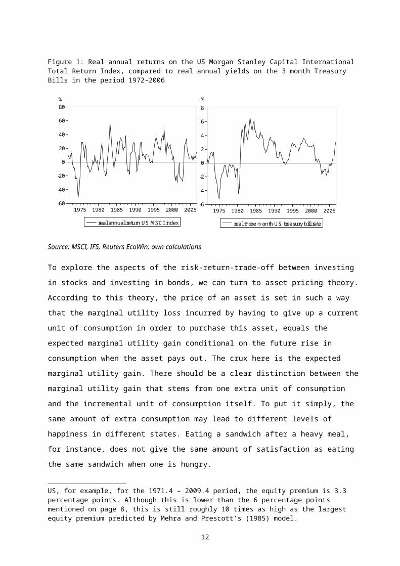
Figure 1: Real annual returns on the US Morgan Stanley Capital International Total Return Index, compared to real annual yields on the 3 month Treasury Bills in the period 1972-2006

-60

-40

-20

0

20

40

60

80

1975 1980 1985 1990 1995 2000 2005

real annual return US MSCI index

-6

-4

-2

0

2

4

6

8

1975 1980 1985 1990 1995 2000 2005

real three month US treasury bill rate

% %

Source: MSCI, IFS, Reuters EcoWin, own calculations

To explore the aspects of the risk-return-trade-off between investing in stocks and investing in bonds, we

can turn to asset pricing theory. According to this theory, the price of an asset is set in such a way that the

marginal utility loss incurred by having to give up a current unit of consumption in order to purchase this

asset, equals the expected marginal utility gain conditional on the future rise in consumption when the

1 While the data in this thesis run until the fourth quarter of 2006, it is important to note that there is still a considerable equity premium when looking at the performance of stock markets after the credit crisis. In the US, for example, for the 1971.4 – 2009.4 period, the equity premium is 3.3 percentage points. Although this is lower than the 6 percentage points mentioned on page 8, this is still roughly 10 times as high as the largest equity premium predicted by Mehra and Prescott’s (1985) model.

8

asset pays out. The crux here is the expected marginal utility gain. There should be a clear distinction

between the marginal utility gain that stems from one extra unit of consumption and the incremental unit

of consumption itself. To put it simply, the same amount of extra consumption may lead to different

levels of happiness in different states. Eating a sandwich after a heavy meal, for instance, does not give

the same amount of satisfaction as eating the same sandwich when one is hungry.

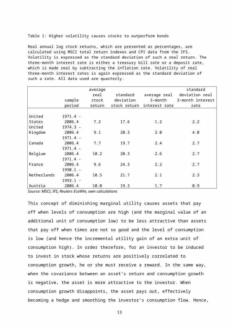
Table 1: Higher volatility causes stocks to outperform bonds

Real annual log stock returns, which are presented as percentages, are calculated using MSCI total return indexes and CPI data from the IFS. Volatility is expressed as the standard deviation of such a real return. The three-month interest rate is either a treasury bill rate or a deposit rate, which is made real by subtracting the inflation rate. Volatility of real three-month interest rates is again expressed as the standard deviation of such a rate. All data used are quarterly.

  sample periodaverage real stock return

standard deviation stock return

average real 3-month interest rate

standard deviation real 3-month interest rate

   United States 1971.4 - 2006.4 7.2 17.6 1.2 2.2United Kingdom 1974.3 - 2006.4 9.1 20.3 2.0 4.0Canada 1971.4 - 2006.4 7.7 19.7 2.4 2.7Belgium 1971.4 - 2006.4 10.2 20.3 2.6 2.7France 1971.4 - 2006.4 9.6 24.3 2.2 2.7Netherlands 1990.1 - 2006.4 10.5 21.7 2.1 2.3Austria 1993.1 - 2006.4 10.0 19.3 1.7 0.9

Source: MSCI, IFS, Reuters EcoWin, own calculations

This concept of diminishing marginal utility causes assets that pay off when levels of consumption are

high (and the marginal value of an additional unit of consumption low) to be less attractive than assets

that pay off when times are not so good and the level of consumption is low (and hence the incremental

utility gain of an extra unit of consumption high). In order therefore, for an investor to be induced to

invest in stock whose returns are positively correlated to consumption growth, he or she must receive a

reward. In the same way, when the covariance between an asset’s return and consumption growth is

negative, the asset is more attractive to the investor. When consumption growth disappoints, the asset

pays out, effectively becoming a hedge and smoothing the investor’s consumption flow. Hence, an

investor will not demand a high return to hold such an asset in his portfolio. (Insurance contracts are

typical examples of these assets. They help investors to smooth their consumption stream, and are

therefore attractive, despite offering a negative rate of return). So, economists generally justify

differences in assets’ returns by examining to what extent a security co-varies with the investor’s

consumption.

The question then is what is precisely the characteristic of an investor’s consumption? The

Capital Asset Pricing Model (CAPM) offers one solution. It presumes that consumption growth of the

investor is perfectly correlated to the return of a broad market index, which acts as a proxy for the state of

the economy. If an asset return is highly correlated to this index (high-beta stock), it is perceived by

investors to be more risky, since it will pay off when the return on the market index is high (and

subsequently when the incremental utility gain for an additional unit of consumption is low).

9

The Consumption Capital Asset Pricing Model (CCAPM) assumes that the investor’s

consumption is perfectly correlated to per capita consumption. According to this model, an asset’s risk is

determined by the covariance of its return with per capita consumption growth. Although the CCAPM is

not as extensively used in real-world applications as its more commercially used counterpart, the regular

CAPM, it is the model of preference from an academic’s point of view.

Table 2 lists the covariance between real per capita consumption growth2 and the real proceeds

from investing in either stocks or bonds for the countries listed in table 1. Stocks are riskier than bonds

not only because they are more volatile, but also because they tend to move more in tandem with

consumption growth. Investors therefore see stocks as a poorer hedge against possible fluctuations in

consumption and will demand a higher premium.

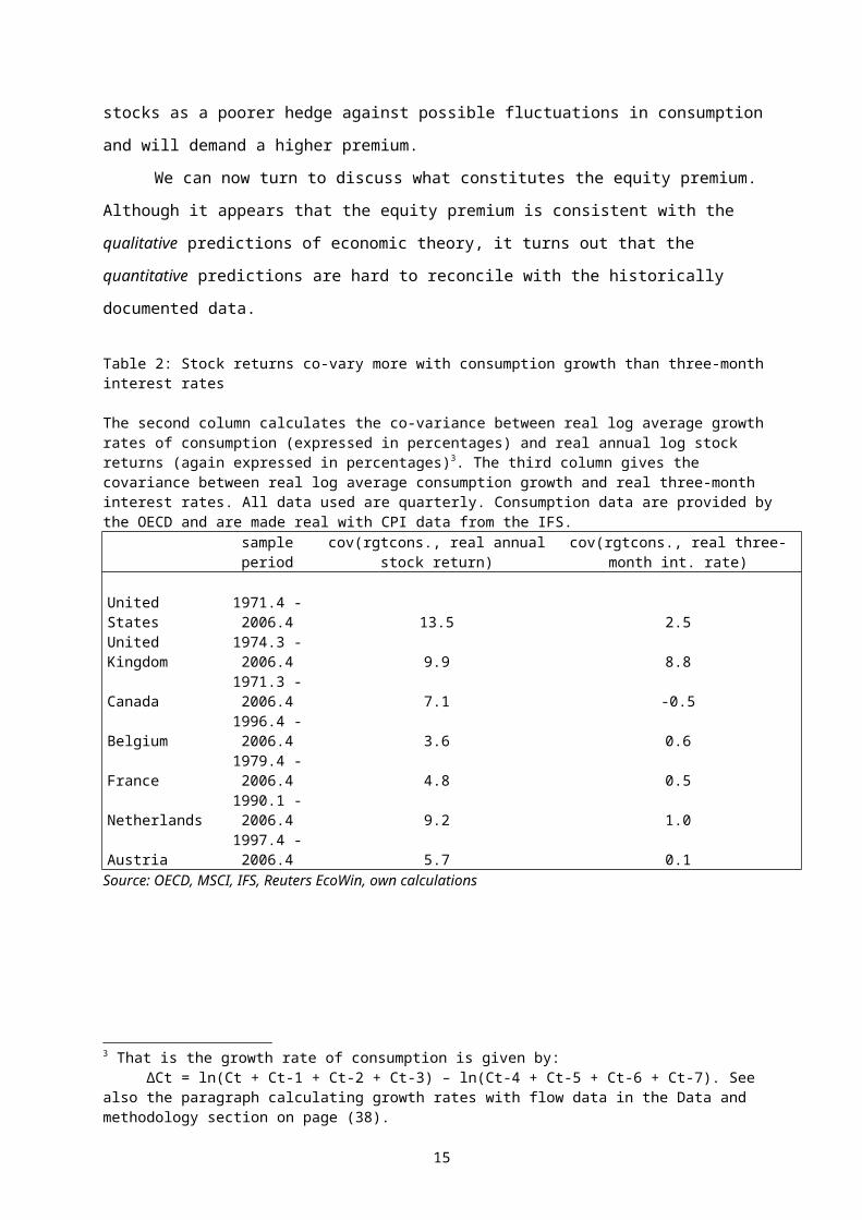
We can now turn to discuss what constitutes the equity premium. Although it appears that the

equity premium is consistent with the qualitative predictions of economic theory, it turns out that the

quantitative predictions are hard to reconcile with the historically documented data.

Table 2: Stock returns co-vary more with consumption growth than three-month interest rates

The second column calculates the co-variance between real log average growth rates of consumption (expressed in percentages) and real annual log stock returns (again expressed in percentages)3. The third column gives the covariance between real log average consumption growth and real three-month interest rates. All data used are quarterly. Consumption data are provided by the OECD and are made real with CPI data from the IFS.  sample period cov(rgtcons., real annual stock return) cov(rgtcons., real three-month int. rate)    United States 1971.4 - 2006.4 13.5 2.5United Kingdom 1974.3 - 2006.4 9.9 8.8Canada 1971.3 - 2006.4 7.1 -0.5Belgium 1996.4 - 2006.4 3.6 0.6France 1979.4 - 2006.4 4.8 0.5Netherlands 1990.1 - 2006.4 9.2 1.0Austria 1997.4 - 2006.4 5.7 0.1

Source: OECD, MSCI, IFS, Reuters EcoWin, own calculations

2.2 Introduction to the puzzles

2 We proxy real per capita consumption growth by estimating real consumption growth. This implicitly assumes that changes in the population are negligible. Although this is not entirely true, i.e. some countries’ populations have grown substantially over time, not taking into account the role of population growth is not likely to alter the results significantly. 3 That is the growth rate of consumption is given by: ∆Ct = ln(Ct + Ct-1 + Ct-2 + Ct-3) – ln(Ct-4 + Ct-5 + Ct-6 + Ct-7). See also the paragraph calculating growth rates with flow data in the Data and methodology section on page (38).

10

2.2.1 The equity premium puzzle

Consider a two-period model, in which a representative agent maximizes a constant relative risk aversion

(CRRA) utility function4:

(1)

where is the parameter of relative risk aversion, with

A key feature of this function is that it connects preferences with time preferences. With CRRA

preferences the coefficient of relative risk aversion is restricted to being the reciprocal of the elasticity of

intertemporal substitution5. This means that a consumer will not only be averse to changes over various

states (i.e. he dislikes risk) but also to changes over time (i.e. he dislikes growth). There is no

fundamental economic reason why this should be, which in itself is an issue that we will revisit later.

To derive total utility from consumption over the two periods, add utility at date 1 to the expected

discounted value of utility at date 2 (calculated as the sum of the utility in a certain state times the

probability of that state discounted by ).

(2)

The parameter is a discount factor being used by investors to estimate current utility from future

consumption. When consumers are impatient (as is only natural to assume). They would rather

receive a unit of utility today than tomorrow. Because of this, is also widely known as the time

preference factor.

The investors’ intertemporal choice problem at time t can be summarized as follows. He compares the

loss in marginal utility related to consuming one real dollar less at period t with the expected discounted

utility gain from investing this dollar in an asset i at time t, selling this asset in period t+1, and

subsequently consuming the proceeds. The marginal utility cost of giving up one dollar of consumption

and investing this dollar into equity is . However, by selling this additional dollar of equity in

period t+1, dollars of extra consumption can be consumed, and

is the expected value of the incremental utility gain, which stems from this additional consumption. The

4 This section leans heavily on Campbell (1998)5 See appendix A.

11

investor reaches an optimum when the marginal cost and benefit equal each other and hence the following

pricing relationship emerges.

(3)

Dividing 3 by gives:

(4)

where is the stochastic discount factor

(5)

Using the definition of the covariance, we can rewrite eq.5 into eq.6

(6)

Combining eq.5 and eq.6 and rearranging the terms gives:

(7)

Note that when the covariance between expected returns and the stochastic discount factor is low, an asset

is perceived to be the most risky. It tends to have low returns precisely whenever marginal utility is high

and the investor values return the most.

Equation 7 has got to hold for all assets including a risk free asset. Since the covariance between

the return on such an asset and the discount factor per definition must be zero, the risk free rate can be

described by:

(8)

12

Assuming that asset returns are conditionally lognormally distributed6, we can take logs of equation 5 and

derive.

(9)

with and , while is the variance of , is the variance of and is

the covariance between and .

Likewise, if we rewrite equation 8 in logs we obtain:

(10)

Notice, that so that . This can be used to rewrite

equation 9 into 11

(11)

where is the variance of consumption growth and is the covariance between and .

and equation 10 into 12

(12)

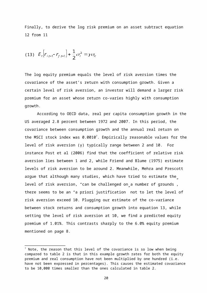
Finally, to derive the log risk premium on an asset subtract equation 12 from 11

(13)

6 When a variable is conditionally lognormally distributed it can be shown to have the following characteristic:

13

The log equity premium equals the level of risk aversion times the covariance of the asset’s return with

consumption growth. Given a certain level of risk aversion, an investor will demand a larger risk

premium for an asset whose return co-varies highly with consumption growth.

According to OECD data, real per capita consumption growth in the US averaged 2.8 percent

between 1972 and 2007. In this period, the covariance between consumption growth and the annual real

return on the MSCI stock index was 0.00107. Empirically reasonable values for the level of risk aversion

(γ) typically range between 2 and 10. For instance Post et al (2006) find that the coefficient of relative

risk aversion lies between 1 and 2, while Friend and Blume (1975) estimate levels of risk aversion to be

around 2. Meanwhile, Mehra and Prescott argue that although many studies, which have tried to estimate

the level of risk aversion, “can be challenged on a number of grounds”, there seems to be an “a priori

justification” not to let the level of risk aversion exceed 10. Plugging our estimate of the co-variance

between stock returns and consumption growth into equation 13, while setting the level of risk aversion at

10, we find a predicted equity premium of 1.01%. This contrasts sharply to the 6.0% equity premium

mentioned on page 8.

A different way to state the puzzle is to examine how large the value of γ in equation 13 should

be in order to match the historical data. It turns out that a risk aversion value of 60.1 is needed to get the

equity premium to reach 6.0%. In order to see just how implausibly high this value is, consider the

following two choices for consumption, for different values of risk aversion8:

What value should X be to make an investor with varying levels of relative risk aversion indifferent

between a gamble over consumption and a certain outcome?

Gamble: $50,000 with probability 0.5

$100,000 with probability 0.5

Certain outcome: $X with probability 1.0

Table 3: The relationship between different levels of risk aversion and X

7 Note, the reason that this level of the covariance is so low when being compared to table 2 is that in this example growth rates for both the equity premium and real consumption have not been multiplied by one hundred (i.e. have not been expressed in percentages). This causes the estimated covariance to be 10,000 times smaller than the ones calculated in table 2.8 Example comes from Mankiw and Zeldes (1991)

γ X1 70,7112 66,6673 63,24610 53,99120 51,85830 51,209

60.1 50,590

14

Clearly, any individual who only wants to pay $50,590 to have a 50 percent chance of winning an

additional $50,000 is highly risk averse.

The level of risk aversion must be set to such a high value, because stock returns offer a large

premium over bond yields, while their covariance with consumption growth is only slightly higher than

the covariance between bond returns and growth in consumer spending. Consequently, an investor needs

to be highly averse to consumption risk in order to be marginally indifferent when choosing between

investing in either stocks or bonds.

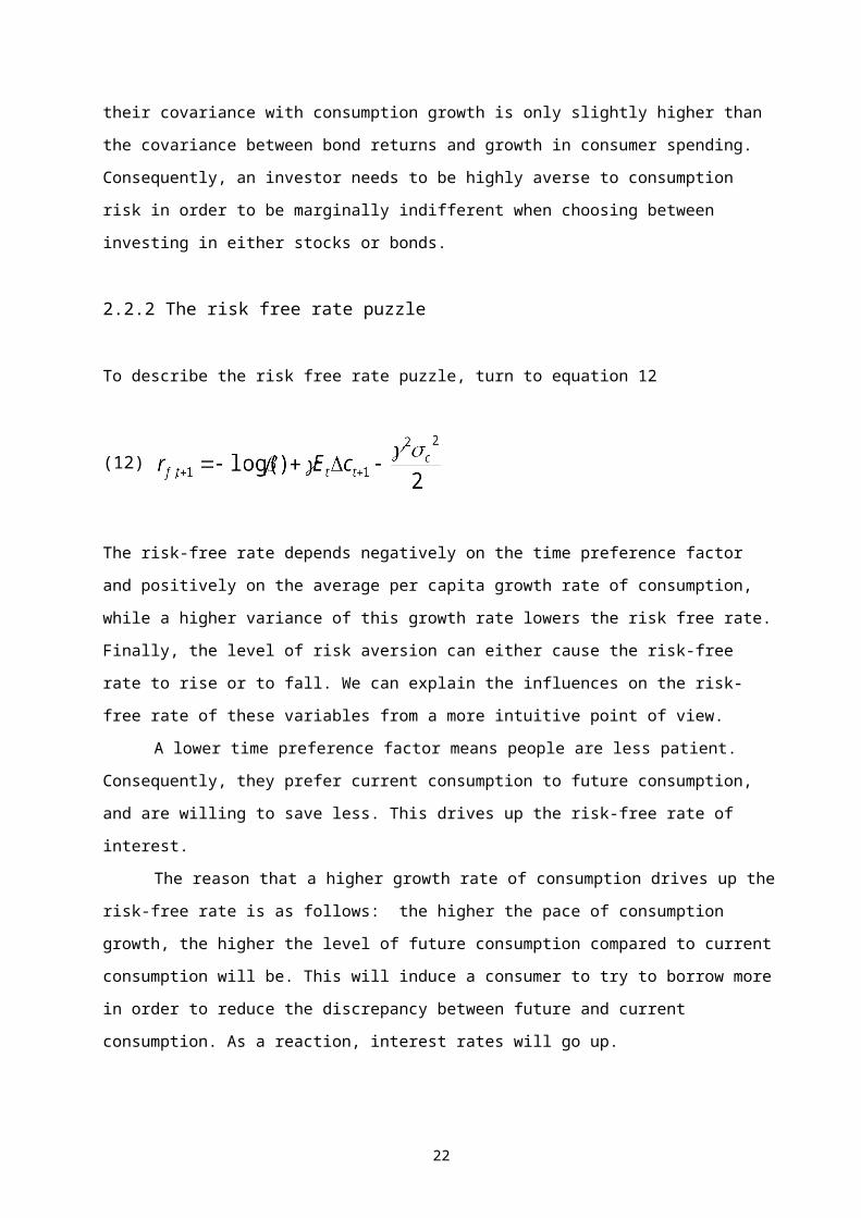
2.2.2 The risk free rate puzzle

To describe the risk free rate puzzle, turn to equation 12

(12)

The risk-free rate depends negatively on the time preference factor and positively on the average per

capita growth rate of consumption, while a higher variance of this growth rate lowers the risk free rate.

Finally, the level of risk aversion can either cause the risk-free rate to rise or to fall. We can explain the

influences on the risk-free rate of these variables from a more intuitive point of view.

A lower time preference factor means people are less patient. Consequently, they prefer current

consumption to future consumption, and are willing to save less. This drives up the risk-free rate of

interest.

The reason that a higher growth rate of consumption drives up the risk-free rate is as follows: the

higher the pace of consumption growth, the higher the level of future consumption compared to current

consumption will be. This will induce a consumer to try to borrow more in order to reduce the

discrepancy between future and current consumption. As a reaction, interest rates will go up.

A higher variance in the growth rate of consumption increases uncertainty about the future. This

added uncertainty will persuade people to save more and as a result, the risk-free rate drops.

The reason that the effect of the level of risk aversion to the risk-free rate is unclear is the

following. The higher the level of risk aversion the higher becomes. This drives up the risk-

free rate. At the same time, an increase in risk aversion will also lower the risk-free rate through the term

in equation 12. It must be said though, that given the low variance of consumption growth the

15

latter will only start to suppress the risk-free rate of interest whenever risk-aversion levels are

exceptionally high, generally exceeding levels around 75. So most of the times, a higher level of will

simply have the tendency to raise the risk-free rate.

To demonstrate this principle, set γ in equation 12 again at 10, and take a value of 0.99 for the

time preference factor. Given that the average variance of real consumption growth in the US was

0.00037 between 1972 and 2007, a value for the real risk free rate of 31.5% emerges. This compares to a

measured real-world value of 1.2%. It is important to understand that the risk-free rate puzzle follows

from the equity premium puzzle. The large level of risk aversion needed to match the equity premium

drives up the risk-free rate in equation 12. As we said before, highly risk averse investors smooth

consumption overenthusiastically not only over different states but also over different time periods. Given

that consumption, in line with the overall economy, grows steadily over time, such risk-averse investors

must borrow in order to reduce the discrepancy between future and current consumer spending. This

results in a counterfactually high demand for money and hence in a modeled risk-free rate, which cannot

be reconciled with actual observed values. Indeed, if we were to use the level of risk aversion found

earlier with the help of equation 13, we would end up with a modeled real risk-free rate of a staggeringly

high 181%.

Another way to look at the risk-free rate puzzle is to see what value the time preference factor

needs to take in order to match the low risk-free rate. In equation 12, a higher value of γ, drives up the

term γEt∆ct+1. This can only be reconciled with the low average real interest rate if the time preference

factor takes a value close to or even greater than 1. This, in turn, corresponds to a low or even negative

rate of time preference. In our example, β needs to be 2.8 to match the average real interest rate,

mentioned at page 8, if the level of risk aversion were to be 60.1 (the level derived with the help of

equation 13). This means that people have a negative rate of time preference and no longer prefer current

consumption to future consumption, i.e. are no longer impatient when it comes to consuming. Intuitively,

if investors are indeed highly risk averse, they dislike an upward sloping consumption profile, and want to

transfer wealth from periods of high consumption to periods of low consumption. However, this will be

offset by the fact that such investors no longer possess the urgency to consume immediately. Whether it is

realistic for people to prefer to delay their consumption expenditures is, however, a highly questionable

presumption.

Section 3: Literature review

3.1 Introduction

This section reviews some of the most important attempts that have been made to explain the high equity

premium and low risk-free rate. The first three sub-sections will focus on three assumptions that have

16

implicitly formed the framework out of which both the equity premium and risk-free rate puzzle have

emerged. Subsection 3.5 looks at some other explanations, while the last subsection addresses the

importance of market segmentation.

3.2 Three common assumptions and the equity premium puzzle

Underlying the results of Mehra and Prescott are three crucial assumptions9. First of all, their model

contains what is known as a “representative agent”, whose utility function is restricted to being of the

constant relative risk aversion class (CRRA, see equation 1). Embracing the concept of such a

representative agent assumes that the behavior of all individual inhabitants in an economy can be proxied

by just one average consumer.

Many economists, though, feel that such a large level of homogeneity is not realistic.

Nevertheless, Constantinides (1982) shows that even when individuals have different preferences and

amounts of wealth, one can create a “composite” consumer, who maximizes a utility function of

aggregate consumption, with the coefficient of risk aversion smaller than the most risk averse individual

and larger than the least risk averse individual. The crux of the matter is that asset markets have to be

complete. As long as there exists a large enough set of assets to diversify away any form of idiosyncratic

risk, individuals, after trading in markets, become homogeneous in their behavior, even if they start out

being heterogeneous.

Additionally, these complete markets need to be totally frictionless. This means that there are no

significant taxes or brokerage fees, no liquidity constraints, nor are there any limitations in knowledge

that may prevent individuals from entering asset markets10. Even if markets are complete, individuals can

only become homogeneous in their actions when there are no significant thresholds that need to be

surpassed in order to enter the asset market. Or put differently, a representative agent can only be created

when individuals have access to complete and frictionless markets.

These three assumptions – i.e. a representative agent with CRRA preferences, who has access to

complete and frictionless markets – have created the framework out of which the equity premium puzzle

– and subsequently the risk-free rate puzzle – have emerged. Not surprisingly, some of the literature has

attempted to resolve both puzzles by weakening one these assumptions.

3.3 Different utility functions

3.3.1 Generalized expected utility

9 Subsections 3.2, 3.3 and 3.4 have greatly benefited from Kocherlakota (1996) The Equity Premium: It’s Still a Puzzle 10 Lack of education is a form of transaction cost, which can cause people to opt not to trade and consequently allocate their assets sub-optimally.

17

The concept of complete markets is deeply rooted in the field of academic economics and many economic

models try to grasp the complexity of real world situations by using a simplifying representative agent. It

is therefore important to see whether the equity premium and risk-free rate puzzles can be resolved

without having to abandon the concept of complete and frictionless markets.

Weil (1989) and Epstein and Zin (1989, 1991) use a set of preferences, which are a generalization

of the standard preference class used by Mehra and Prescott. In these “Generalized Expected Utility

preferences” (GEU) the coefficient of risk aversion and the elasticity of intertemporal substitution can be

parameterized independently. With GEU preferences, the level of risk aversion is given by , while

describes the elasticity of intertemporal substitution. The normal power utility function emerges

when .

(14)

Weil shows that if one disentangle the coefficient of risk aversion and the elasticity of intertemporal

substitution, the magnitude of the equity premium is determined by , while the risk-free rate is being

controlled by . The former has to do with volatility, while the latter is linked to average consumption

growth. Although these properties can be exploited to match the historical risk-free rate and equity

premium almost perfectly, this continues to rely on unrealistically high levels of risk aversion. If one uses

a more realistic risk aversion level, the model is no longer able to replicate the historical data11. In a way,

this is a more significant breakdown than when Mehra and Prescott’s power preferences were imposed.

No longer can the failure of the model be attributed to its disability to govern the level of risk aversion

and the elasticity of intertemporal substitution independently. This leads to the risk-free rate puzzle. The

risk-free rate is simply too low to match average per capita consumption growth, if individuals were to be

highly averse to intertemporal substitution.

Nevertheless, Kocherlakota (1996) and Mehra (2003) argue that imposing GEU preferences can

be beneficial in resolving the risk free rate puzzle. The big advantage of these preferences is that when a

consumer is highly risk averse, he or she no longer necessarily wants to smooth consumption over time.

This reduces the incentive to borrow and therefore should mitigate the risk free rate puzzle. Indeed, while

the level of risk aversion and the elasticity of intertemporal substitution need to be high simultaneously in

order to replicate the historical data, the independent parameterization does increase the ability of the

model to deal with the historically high consumption growth.

Turning to the equity premium, Epstein and Zin’s paper strikes a positive note as well. They

claim to have resolved the equity premium puzzle, by implementing GEU preferences. However, their

results appear to be sensitive to empirical design. Testing a utility function with GEU preferences is

11 I.e. you would need an unrealistically high level for the elasticity of intertemporal substitution to replicate the data.

18

difficult, since utility in period t partly depends on the unobservable utility in period t+1. To proxy this

unobservable utility one needs the help of instrument variables. These require detailed assumptions about

the underlying consumption process, which do not necessarily need to describe the actual consumption

process. As a result, the claim that Epstein and Zin have resolved the equity premium puzzle may be

overstated (Mehra 2003). In addition, Kocherlakota (1990) shows that the problem of unobservable utility

in period t+1 can easily be sidestepped, when one takes into account that it is difficult to predict future

consumption growth using currently available information. She therefore assumes that consumption

growth is statistically independent of all the information used by the investor and that the growth rate of

consumption is i.i.d.. In this case, it can then be shown that a utility function with GEU preferences does

not have more explanatory power than the normal power utility function.

3.3.2 Habit formation

A second modification in the preference structure includes habit formation in the utility function.

Constantinides (1990) argues that utility is not only affected by current consumption expenditures but

also by past levels of consumption. It may be more natural to think that once an individual becomes used

to a certain level of consumption, he or she will perceive future levels of consumption in the light of this

earlier level. To put it simply, if a person consumed a lot yesterday, it takes more consumption today to

make such a person happy.

This property of intertemporal preferences can be given by the following formula:

(15)

where utility increases once a certain subsistence level of consumption is passed ( ), which is given by

an exponentially weighted sum of past consumption (see also Constantinides (1990)).

This utility function makes the representative agent highly averse to movements in consumption, even if

his initial level of risk aversion is low. People who have habit persistence are more sensitive to changes in

consumption, since any change in consumption increases the chance of it falling below the subsistence

level. Small changes, therefore, can lead to large changes in marginal utility. Constantinides (1990)

argues that habit formation solves the equity premium puzzle, while Abel (1990) is able to generate a

reasonable equity premium with a model that uses a low level of risk aversion and a utility function of the

form presented above. Kocherlakota (1996) and Mehra (2003), on the other hand, are not convinced,

claiming that although consumers can have a lower coefficient of risk aversion, they remain implausibly

averse to changes in consumption in general.

19

Habit formation does, however, help to mitigate the risk-free rate puzzle. In the habit formation

framework people are more inclined to save. For any level of consumption at time t, the agent is aware of

the fact that his demand for consumption in the future will be higher, since his perception of future

consumption is habit forming. This, in turn, makes the consumer more willing to save, driving down

interest rates.

A different approach has been taken by Campbell and Cochrane (1999). They use a model with

varying levels of risk aversion, which incorporates habit formation, and in addition takes the possibility of

a recession as a state variable. Risk aversion increases considerably during periods in which the

probability of a recession is high. Consequently, stock prices fall and their expected return increases.

Thus the model is able to explain a high equity premium. Moreover, in times of recession, consumption

tends to decline to its subsistence level. This leads to precautionary savings, which in turn ameliorate the

risk-free rate puzzle. Although the model is consistent with both consumption and asset market data, it

does require huge countercyclical, time-varying levels of risk aversion. The main contribution of

Campbell and Cochrane’s article, therefore, is not a resolution of the equity premium puzzle. They do,

however, show that risk is time-varying and business-cycle dependent and better explained by a utility

function which exploits habit formation.

3.3.3 Catching up with the Joneses (relative consumption)

The standard utility function, used in the Mehra and Prescott framework, presumes that people only

derive utility from their own consumption. The third set of preference modifications, in contrast, assumes

that an individual not only obtains utility from his or her own set of consumption goods, but also from

whether he or she consumes more or less than an average consumer one period ago. Thus an individual

derives his or her utility by looking at his or her own consumption level and then compares this to the

level of average per capita consumption one period ago. This form of utility function is labeled by Abel

(1990) as “catching up with the Joneses” 12.

(16)

where is the investor’s own consumption in period t and is aggregate consumption per capita in

period t.

12The phrase “catching up with the Joneses”, rather than “keeping up with the Joneses”, reflects the fact that consumers care about the lagged value of per capita consumption (see also Abel 1990). In contrast, some researchers e.g. Gali (1989) have investigated a utility function in which the investor derives his utility by comparing the current level of his consumption with the current level of per capita consumption.

20

The consequence of this modification is that the consumer, once again, becomes hugely averse to

movements in consumption, since any variation can drive his or her consumption stream below that of his

or her peers. Abel (1990) shows that this model is able to generate an equity premium of 463 basis points

and a risk free rate of 2.07 percent with a level of risk aversion no higher than 6.

However, Kocherlakota (1996), using a slightly different utility function, argues that instead of

being implausibly averse to his or her consumption risk, a consumer’s marginal utility of his own

consumption now depends too strongly on variations in per capita consumption. Consumers therefore

become highly averse to fluctuations in societal consumption. Hence, although a large equity premium

can be reconciled with relatively low levels of risk aversion, in essence, unrealistically high levels of

individual risk aversion are substituted with unlikely levels of risk against changes in the average

consumption level of the economy.

Mehra (2003) nevertheless argues that this relative utility function is able to take the edge off the

risk-free rate puzzle. Since average consumption rises over time, individuals want to “catch up” with

others. Equity therefore becomes an unattractive asset, since unfavorable changes in stock prices can

drive an individual’s consumption stream below that of his peers. This in turn drives up the demand for

bonds and consequently lowers the modeled risk-free rate.

In sum, attempts up till now to solve the equity premium by modifying the utility function of the

representative agent have proven to be largely unsuccessful, while they have had some successes in

resolving the risk-free rate puzzle. Generally, two distinct points can be made. Firstly, the risk-free rate

puzzle can be solved, or at least mitigated, if the attitudes in the preference function towards risk and

growth are to be disentangled.

Secondly, the equity premium puzzle has proven to be much more challenging. Consumption

tends to grow smoothly and consequently does not co-vary much with returns on stocks. Still, investors

keep on demanding high premiums for investing in stocks relative to government bonds. The only reason

left in a framework that incorporates a representative agent model is then that of an investor who is

indeed highly averse to changes in either individual consumption or societal consumption.

3.4 Incomplete markets and trading costs

It is hard to imagine that markets are fully complete so that individuals can insure themselves completely

against all potential changes in their consumption streams. It is particularly difficult to get insurance

against changes in human capital, which for most people determines the lion’s share of their wealth and

therefore their present and future levels of consumption. For this reason, many economists doubt whether

markets are truly complete. Moreover, although the implementation of technological trading systems has

greatly reduced trading costs, most investors continue to be confronted with expenses when they give

21

their orders. Not only do these outlays include brokerage fees, but they also comprise information costs,

borrowing constraints, an inability to take short positions, taxes, bid ask spreads, management fees etc.

Consequently, a complete insurance package may not be available and hence the individual

consumption stream may include risks that are not present when consumption is proxied by per capita

consumption. Accordingly, models with incomplete markets “hope” that individual consumption growth

will be more volatile than aggregate per capita consumption growth and hence will co-vary more with

stock returns. Such models would then not require the implausibly high levels of risk aversion seen with

complete market models.

Throughout the following sub-section, all investors are assumed to posses the standard utility

function, used in the Mehra and Prescott model, and given by eq. 1. The challenge now is to see whether

any research has succeeded in solving either the equity premium or risk-free rate puzzle by focusing

solely on the incompleteness of markets and trading costs (and not as in the previous section by

concentrating on different preference structures).

3.4.1 Idiosyncratic income risk, which cannot be insured

In infinite horizon models, individuals who cannot insure themselves successfully against temporary

income shocks will dynamically self-insure. Because the utility function is concave, they will purchase

bonds and stocks in prosperous times to create a buffer against future income shocks, while selling them

when they sail into headwinds. This smoothes their consumption pattern so it will turn out to be very

similar to the pattern that would emerge under the complete market framework. Consequently, the equity

premium in an incomplete market setup should be broadly the same as the equity premium in a complete

market.

This intuitive argument is confirmed by the numerical work done by Heaton and D. Lucas (1995).

They construct an infinite horizon economy, which involves two groups of people, both of which are

susceptible to systematic labor risk and idiosyncratic labor income risk, and which is calibrated with the

help of the US Panel Study of Income Dynamics. They show that when costless trading is allowed,

temporary idiosyncratic income shocks are offset by trade in assets. Consequently, the equilibrium asset

prices are broadly similar to the predictions of the Mehra and Prescott model.

The argument, however, changes if labor income shocks become permanent (Constantinides and

Duffie (1996)). Due to the permanence of the shock, one can no longer temporarily deplete once savings

in order to smooth consumption. As a consequence, the magnitude of the shock will be fully reflected in a

constant lower level of consumption. In such circumstances, it is impossible to dynamically self-insure

with the help of asset markets. Individual consumption growth will therefore deviate more than per capita

consumption growth and a large equity premium is warranted, with lower levels of risk aversion.

The subsequent step is then to test whether income shocks are indeed permanent. Unfortunately,

due to data constraints, this is a difficult issue to sort out. Nevertheless, Heaton and D. Lucas (1995),

22

using data from the US Panel Study of Income Dynamics, estimate the autocorrelation of income shocks

to be 0.529. So based on – admittedly meager – empirical research, individual income shocks appear to be

nonpermanent (stationary) and the incomplete market setup will most likely not lead to a resolution of the

equity premium puzzle.

With regard to the risk-free rate puzzle, the arguments are broadly similar as the ones presented

above. Although individuals should have a demand for precautionary savings when confronted with

income shocks, this demand declines when individuals “live” in an infinite horizon economy. They, then,

will dynamically self-insure. This suggests that the extra demand for savings in an indefinite incomplete

economy is relatively small. Consequently, the difference between the incomplete and complete market

interest rate should also be small.

3.4.2 Trading and Transaction costs

Although there may be a contingency for every state of the world and hence the possibility to insure

oneself perfectly against adverse events, this may prove to be too costly in reality. Transaction costs could

therefore trigger the individual consumption stream to fluctuate more than average per capita

consumption, justifying a high equity premium.

Interestingly, in Heaton and Lucas’ experiment, whenever the modeled transaction costs are

increased, the average bond return falls, while there are no noticeable changes in the returns on stocks.

Consequently, the equity premium widens. Precisely when this happens, trade volumes fall and the

standard deviation of consumption growth rises, in turn raising the covariance of individual consumption

growth with returns on stocks. So apparently, the model is able to prevent agents from dynamically self-

insuringe. However, Heaton and Lucas impose unrealistically high transaction costs. To get the model to

derive an equity premium of 5 percent, one requires transaction costs of 10 percent to trade in stocks, or

when imposing transaction costs for both bonds and stocks, an average cost of transaction of 5 percent for

stocks and 2 percent for bonds. So, even though the model does reveal some interesting aspects of

incomplete markets, i.e. it becomes more difficult to insure oneself dynamically when transaction costs

rise, it fails to explain the equity premium seen in markets today.

Aiyagari (1993) sees a completely different role for transaction costs. In his model, by

assumption, trading in stocks involves having to pay transaction fees, while trading in bonds is costless.

This accounts for a large equity premium in two ways. Firstly, individuals, when confronted with

incomplete markets and hence with income uncertainty, hold precautionary savings in order to smooth

consumption when times are bad. This reduces the risk-free rate. Secondly, in order to compete with

bonds, stocks, which are assumed to be without risk, must pay an additional premium, since they bear

transaction costs. This, then, drives up the returns on stocks. Together, these effects account for a large

equity premium.

23

But it seems dubious that this way of reasoning can lead to a solution to the equity premium

puzzle. There is no proof that trading in stocks demands higher transaction costs than trading in bonds.

Moreover, letting transaction costs account for the equity premium in such a way collides with all our

earlier beliefs about risk and the potential rewards that follow from taking it. A solution for the equity

premium puzzle must be found in understanding how individuals perceive risk and its subsequent

rewards, not by linking differences in transaction costs to differences in returns.

To summarize, although incomplete market models look promising at first, and admittedly, are

easier to be reconciled with reality, they fail to solve both the equity premium and the risk-free rate

puzzle. When confronted with income uncertainty, individuals simply insure themselves dynamically. As

a result, their consumption pattern approaches the same amount of smoothness as seen with representative

agent models, and consequently the difference between asset prices in incomplete and complete market

models is small. Adding transaction costs does not seem to change this. One needs to raise levels of

transaction costs to unrealistically high levels for a reasonable equity premium to emerge. When making

trading in stocks significantly more expensive than trading in bonds though, an equity premium, as the

one observed in reality, materializes. However, this premium has nothing to do with bearing risks, and

occurs solely as compensation for differences in transaction costs.

3.5 Other explanations

3.5.1 Transaction services return

Bansal and Coleman (1996) try to find a solution for the equity premium puzzle, by looking at the

transaction service component of different assets. In their model, it is presumed that assets other than

money have a distinct function in helping to facilitate transactions which has an effect on their offered

rate of return. They argue that, in equilibrium, the transaction service returns on cash relative to checking

deposits should equal the nominal interest rate paid on these deposits. In order to analyze the transaction

service return of different assets, they develop a monetary economy that distinguishes between payments

by cash, credit and checks. In their model, the risk-free asset offers a transaction services return and this

affects its market value. So, as long as bonds have larger transaction services components than stocks,

investors may demand a higher return for holding stocks to compensate. This could explain the equity

premium witnessed in the markets.

Mehra (2003), however, challenges their reasoning. First of all, the majority of government bonds

are held by institutions for investment purposes, making it difficult to understand that these institutions

would accept lower returns in order to benefit from the alleged services returns offered by these bonds.

Secondly, the model predicts a substantial yield spread between short-term Treasury bills and long-term

government debt, since the latter presumably cannot offer any transaction services. This, however, is not

seen in practice.

24

3.5.2 Survival bias

Brown, Goetzmann and Ross (BGR) (1995) focus on survival bias to explain the high equity premium.

All empirical work in finance is conditioned upon the availability of data. But, as the argument goes, this

implicitly forces researchers to study only data from exchanges that have survived for a considerable

amount of time. As a consequence, there is the probability that these exchanges’ data are “formed” by

price paths that would not have emerged if the exchanges had ceased to exist due to adverse events. Or

put differently, the equity premium is high because the data that underlie this premium are biased towards

survival. The available equity premiums are therefore only a sub-set of the total sample and paint too

positive a picture about the “true” returns on stocks.

However, this line of reasoning can raise serious questions. For a start, the high equity premium

is not restricted to one country. In fact, financial data show that stocks tend to pay substantially higher

returns than bonds in many countries (see also table 1). What’s more, Li and Xu (2002) argue that BGR’s

model is fundamentally flawed. It assumes an unrealistically high probability of market failure. In short,

their reasoning goes as follows: the market survives as long as the stock price stays above a certain

absorption barrier. The probability of a failing market therefore is only high at an early stage of the

market, when the difference between the stock price and the barrier is small. Under the presumption that

stocks, on average, rise in value, the price will continue to move away from the absorption barrier as long

as the market survives. At a certain point, the price of the stock will be so much higher than the barrier

that the chance of crashing into it almost completely disappears. With the probability of a market failure

declining to zero, the distribution of stock prices, conditioned upon market survival, will be very close to

the unconditional distribution, and the bias in the data due to survival will be negligible. Or intuitively,

the longer the exchange stays in business, the more reliable the data, since the exchange has lived though

many periods in which there has been a high chance that exchanges, which had just started, would have

failed.

3.5.3 Disaster States

Rietz (1987) argues that the high equity premium reflects compensation demanded by investors against a

small probability of an extreme market crash. Although these kinds of crashes have never been observed

in reality, investors may simply account for the fact that there is always a small chance of an economic

catastrophe. Rietz re-specifies Mehra and Prescott’s model so that it captures the effects of possible, but

highly unlikely, collapse in the stock market due to a catastrophic event13. This brings down the risk-free

rate, while the model is able to explain a high equity premium with a reasonable degree of risk aversion.

13 More precisely, he adjusts the transition probability matrix so that there are three states in the world. A good and bad state, and a highly improbable one-time crash. This compares to Mehra and Prescott’s original two-stated model, which has only a good and a bad state.

25

Interestingly, in Rietz’s model the coefficient of risk aversion decreases when the chance of a massive

stock crash increases.

However, Rietz’s results rely on adding a huge amount of risk to the economy, which may well

prove to be unrealistically high. The smallest annual decline in consumption in his model is 25%. This

means that investors speculate that there is a possibility that consumption in one year may drop by an

amount, which roughly equals the entire fall in consumption seen during the Great Depression in the US

in the 1930s14. To put this number into some perspective, in the US the peak-to-trough decline in private

consumption during the recession in the 1980s was 2.4%, while during the latest recession consumption

only fell by a cumulative 1.95%15. It would therefore take an unprecedented shock to the economy – like a

war – to arrive at the declines that Rietz proposes. Moreover, the consequences of an extreme market

event only affect stocks, while hypothetical catastrophes also should have an impact on bonds (Mehra

(2003)). In times of stress, when governments fail to meet their debt obligations, or try to reduce the real

value of their debt by creating unanticipated inflation, both stocks and bonds are likely to suffer

simultaneously. As a result, the consequences for the equity premium itself should be relatively small.

Additionally, Mehra and Prescott (1988) claim that historical confirmation is needed to support

Rietz’s hypothesis. If the probability of an extreme adverse economic event rises, investors should

channel their money into safer assets and consequently real yields should drop. Focusing on two events,

evidence for this proposition is mixed. During the Cuban Missile Crisis in 1962, a period when the

likelihood of a nuclear war between the US and the former Soviet Union reached its peak, real rates

remained stubbornly high. More recently, however, we have seen a steep drop in real yields, as the near-

collapse of the financial system, precipitated by Lehman Brothers’ bankruptcy in September 2008, led to

huge safe-haven flows.

3.5.4 Myopic loss aversion an the equity premium puzzle

Bernatzi and Thaler (1995) look at the aspects of behavioral finance to find an explanation for the large

difference between stock and bond returns. They combine two concepts of Kahneman and Tversky’s

prospect theory (1979): loss aversion and mental accounting. The first relates to the tendency of

individuals to be more sensitive to losses in their wealth than to increases (the utility function is convex

for losses, while being concave from profits). Mental accounting, meanwhile, refers to the methods

individuals use to evaluate investment results. Bernatzi and Thaler combine those two concepts into

14 In fact, real consumption declined by 18% between 1929 and 1933.15 According to the NBER’s Business Cycle Dating Committee there were two recession in the 1980s. The first started in 1980Q1 and ended in 1980Q3, while the second began in 1981Q3 and ended in 1982Q4. The 1980Q1-1980Q3 recession in particular was characterized by a steep downturn in consumption, with a peak-to-trough decline of 2.4% (hence this is the number, which is mentioned in the text). The second recession in the 1980s, in contrast, only saw a peak-to-trough decline in consumption of 0.8%, reflecting that this recession was more driven by weak investment. In addition, the NBER’s Business Cycle Dating Committee decided that the latest recession in the US started in the fourth quarter of 2007. Assuming that this recession ended in 2009Q2, the cumulative drop in consumption between 2007Q4 and 2009Q2 was 1.95%

26

“myopic loss aversion”. Loss averse investors are reluctant to evaluate their portfolios frequently, because

at each evaluation there is the probability of a decline in value. Because of this, the amount of risk

investors are willing to take depends on the frequency of evaluation. Even if a high-yielding asset is

perceived to be the better investment in the long run, investors might opt not to purchase it, since it is

more risky and hence there is a bigger probability that a loss turns up during an evaluation in the short

run. As a result, as long as an investor is not forced to reveal his results, riskier assets become more

attractive. This behavior leads investors to demand a higher premium for having to invest in risky stocks

when the frequency of evaluations increases. Thus, the equity premium in this context should be seen as

compensation for having to evaluate one’s investments frequently and not as compensation for risk in

more general terms.

In line with the reasoning above, Glassman and Hassett (1999) suggest that investors mistakenly

perceive short-term volatility in stock returns as long-term risk. This in combination with the fact that

investors are loss-averse accounts for the high equity premium.

Whether the solution for the equity premium puzzle can truly be found in behavioral finance is

questionable. Despite their intuitively appealing reasoning, the actual evidence presented by Bernatzi and

Thaler is meager. In essence, their model, which uses a utility function, as shown in equation 17, shows

that the equity premium does indeed shrink whenever the evaluation intervals are lengthened.

(17) for and if see also Bernatzi and Thaler (1995)

More precisely, when investors look at the performance of their investments once a year, the model is

consistent with a premium of 6.5%. They then claim that since this is a plausible result, – i.e. investors

have to file taxes annually and have to inform clients about their performance on an annual basis – there

is no reason for the large equity premium to be a puzzle.

However, the equity premium puzzle has arisen only because of economists’ previous belief

about CRRA utility functions. Changing the utility function to a function that is consistent with the

Prospect theory does not, therefore, solve the puzzle.

More fundamentally, if the equity premium is indeed a reward for “evaluation risk”, there should

be great arbitrage possibilities. By checking one’s performance less frequently than others, while

investing in the same assets, investors can easily make a higher return than they need to, given the length

of their evaluation period. There should therefore be a continuous tendency in the market to widen

evaluation periods, and consequently the equity premium should decrease rapidly. Although Blanchard

(1993) argues that the equity premium has recently fallen, the drop is in no way consistent with the

reduction in the premium that would occur, if the equity premium stemmed solely from “evaluation risk”

instead of normal risk.

3.6 Market segmentation

27

3.6.1 Unequal distribution of income and wealth

Edward Wolff (2000), using data from the Survey of Consumer Finances, shows that in terms of wealth

distribution in the US, the richest 5% owned more than 68% of all financial wealth (that is wealth

excluding home equity) in 1998, while the top 20% accounted for almost 91% of financial wealth.

This uneven distribution of wealth and income also affects stock ownership. Haliassos and

Bertraut (1995), using data from the same survey as Wolff, show that as a proportion of total personal

wealth, people tend to hold more stocks when their income is higher. Given the unequal distribution of

income, they estimate that between 75% and 80% of all United States households do not hold stocks

directly, while – when the indirect holdings of stocks through pension funds are considered – not more

than 36.8% of all families in the US hold stocks.

These results are confirmed by Mankiw and Zeldes (1991), who, with the help of data from the

Panel Study of Income Dynamics, show that in 1984 only 27.6% of all families surveyed held a positive

amount of their wealth in stocks. Although the question of why so few people hold stocks is another

puzzle in itself16, the incidence of stock ownership seems to be mostly correlated with the level of

education and wealth. The former has to do with transaction costs: lack of knowledge and plain ignorance

poses a significant barrier to entering into trade. The latter results from big inequalities in the distribution

of income and wealth.

A look at table 4, which presents Gini coefficients for a range of different developed economies,

shows that although the US is by far one of the most unequal countries, other developed economies have

relatively unequal income distributions as well.

Table 4: Gini coefficients for different developed economies in 2007

The Gini coefficient measures the equality of the income distribution of an economy. It is defined as a ratio between 0 and 100. 0 corresponds to perfect equality, while 100 refers to perfect inequality (that is one person earns the total country’s income).

US UK Canada Belgium France Netherlands Austria45 34 32 28 28 31 26

Source: CIA World Factbook

This suggests that the same pattern of stockholders’ distributions as found in the US will also be visible in

other developed economies. Indeed, Attanasio et al (2002) show that in the United Kingdom, the

proportion of households which owned shares varied between 8 and 24 percent in the period 1978 - 1995.

With such a large part of society not owning stocks, it becomes hard to continue to embrace the concept

16 It is a puzzle, because even a person with a low income or wealth level can increase his maximum amount of utility during his life span if he invests in stocks. It is even more difficult to explain the conclusions of Mankiw and Zeldes’ (1991), whose results show that of those consumers who hold assets in excess over $100,000 only 47.7% invest in stocks.

28

of a complete market with a representative agent, whose consumption growth can be proxied by

aggregate per capita consumption growth. Moreover, although Heaton and Lucas (1995) show that the

difference between the equity premium in an incomplete market setup and a complete one is small, this

requires that all participants in the economy are capable to dynamically self-insure themselves against

adverse events through the trade in assets. However, the uneven distribution of incomes in developed

countries and the empirical work done by Wolff and others suggest that most people in these countries

simply do not have the means to purchase assets and hence that such a form of insurance is not available.

An objection to the empirical work on consumption asset pricing models is therefore that it

proxies the representative investor’s consumption stream by aggregating both the consumption of

stockholders and non-stockholders17. Indeed, if one wants to determine consumers’ risk aversion, one

should only look at those consumers whose consumption is actually affected by changes in the prices of

stocks. In essence, there is no a priori reason to expect someone who does not own an asset, to adjust his

or her consumption stream in response to anticipated changes in that asset’s price. Working in the other

direction, consumption patterns of investors who do own assets are likely to be more volatile and

correlated to stock returns, since changes in volatile stock markets are likely to have an effect on their

consumption behavior. If so, the estimated level of risk aversion of those consumers who actually invest

is likely to be lower than for those consumers who do not own stocks. This suggests that market

segmentation may be possible. If only a subset of consumers actively participate in capital markets,

estimates of risk aversion are no longer valid when one looks at the relationship between aggregate

consumption growth and stock returns, since aggregate consumption includes the consumption of both

stockholders and non-stockholders.

3.6.2 Market segmentation

Mankiw and Zeldes (1991) were the first to explore this concept. Unfortunately, their use of data leaves

serious room for improvement. To examine the differences between consumption growth of stockholders

and non-stockholders, they investigate the amount of money spent on food (both at home and in

restaurants), with the help of data from the PSID survey. Besides the fact that food expenditure may not

accurately reflect total consumption, their data only consists of 13 annual observations of growth rates,

while – as is usually the case with survey data – it is likely to contain serious measurement errors. Despite

17 Note, that in the incomplete market models discussed on pages 21 to 24, the consumption of both stockholders and non-stockholders is also aggregated. Although these models show that consumers will insure themselves dynamically in the absence of complete markets, models that distinct between the consumption of stockholders and non-stockholders assume that those who do not hold stocks, by definition, do not participate in the trade of assets and therefore automatically will not be able to insure themselves dynamically. In other worlds, not trading in assets will force the non-stockholders to live in an “incomplete” world. In contrast, the stockholders will live in a “complete” world, either because they have access to complete markets, or, when markets are not complete, they are able to insure themselves dynamically. While living in a “complete” world is likely to reduce fluctuations in consumption growth, this is offset by the fact that stockholders’ consumption growth is affected by changes in volatile stock markets. This actually causes the standard deviation of their consumption growth to be higher than the standard deviation of non-stockholder’s consumption growth (see table 7 in Section 5).

29

the poor quality of the data, their findings are encouraging. They show that consumption growth of

stockholders is more volatile and more correlated to stock returns than the consumption of non-

stockholders, suggesting that part of the equity premium puzzle has indeed been caused by the unjustified

aggregating of consumption expenditure of both stockholders and non-stockholders.

The importance of market segmentation is also underlined by the results of Vissing-Jørgenson

(2002), Brav, Constantinides and Geczy (2002) and Attanasio, Banks and Tanner (2002). Like Mankiw

and Zeldes, these researchers all base their conclusions on the use of survey data. Vissing-Jørgenson

shows the elasticity of intertemporal substitution to be statistically different for asset holders and non-

asset holders. Meanwhile, Brav et al show that when one takes into account limited stock market

participation, i.e. only looks at those households that own stocks, the market for stockholders possesses

some form of completeness. Moreover, they show that when the definition of being a stockholder is

tightened, the risk aversion level of such an investor declines. This suggests that it is not only important to

distinguish between asset holders and non-asset holders, but also that the portion of a household’s wealth

invested in the stock market determines the level of risk aversion.

The results of Attanasio et al underscore the relevance of making a distinction between

stockholders and non-stockholders as well. They, however, present one interesting innovation. A

drawback of the use of survey data in general is that researchers have the tendency to treat owning stocks

as a permanent state. Mankiw and Zeldes for instance define groups of stockholders and non-stockholders

on the basis of share ownership in the last period of the sample. This implicitly assumes stock-ownership

to be a permanent choice. However, according to both US and UK data, the share of stockowners in the

population has changed markedly over recent years. To take into account that consumers may start to

become stockholders (or that stockholders stop investing) Attanasio et al select a number of demographic

and economic variables that are used to predict whether a household owns stocks or not. As seen in other

research, the likelihood of being a stockholder increases with age, suggesting that once people have

gathered some wealth they start to participate in the stock markets, while a higher level of education also

increases the probability of share ownership. Their results once more indicate that making a distinction

between those who possess shares and those who don’t is vital. Consumption growth for stockholders is

much better correlated to stock returns than for non-stockholders, suggesting that estimates of risk

aversion for non-stockholders are biased upwards.

Constantinides, Donaldson and Mehra (2002) combine the concept of consumer heterogeneity

with borrowing constraints. In their article Junior Can’t Borrow, they model an overlapping generations

economy, which incorporates a life cycle feature to study asset prices. The attractiveness of investing in

stocks depends on the state in the life cycle of an individual. A young consumer has not yet enjoyed the

possibility to build up wealth and consequently his consumption will be mostly financed out of labor

income. For such a person, stock returns will not co-vary greatly with consumption growth. Equity will

therefore be an effective hedge against variations in labor income and thus an attractive asset to have in a

portfolio. The characteristics of the same stock investment though are totally different for middle-aged

30

consumers. These consumers have much smaller wage uncertainty than their younger counterparts, while

they have had the chance to save for retirement. Their future pension income will be almost completely

determined by their investment income. The changes in their consumption patterns will therefore be much

more related to changes in the performance of stock markets. Equity no longer functions as a hedge

against changes in consumption. When stocks perform well, consumption will also do well and vice

versa. As a consequence, a middle-aged consumer will demand higher rates of return for having to

channel his savings into the stock market.

The crux of Constantinides et al’s model is that the young consumers are shut out of the equity

market because they face considerable borrowing constraints. Since it is difficult to collateralize loans

with human capital, their limited level of financial wealth prevents them from having access to debt

markets. Accordingly, the “pricing” of stocks is left to the middle-aged consumers, who perceive stocks

as an undesirable asset. The return on stocks and hence the equity premium is therefore high, while the

reason that the young have no access to debt causes the rate of interest to be low.

Interestingly, whenever the borrowing constraints are relaxed, young consumers start to borrow.

This raises interest rates, which, in turn, induces the middle-aged consumer to invest more in bonds.

Meanwhile, young consumers will use part of their borrowed money to invest in equity. This increased

demand for stocks by the young consumers will be partly offset by reduced demand from the middle-aged

consumers. But on balance, the effect of lifting the borrowing constraints causes the returns on both

stocks and bonds to increase, reducing the equity premium.

To summarize, both wealth and income are unequally distributed among the inhabitants of

developed economies. As a consequence, the majority of consumers do not own stocks. Assessing their

level of risk aversion by looking at how patterns in their consumption are affected by fluctuations in the

stock market does not, therefore, make sense at all. If a consumer does not own stocks, his or her

consumption pattern will not be affected by fluctuations in the stock market. Asset pricing models should

therefore strictly focus on the relationship between spending growth of consumers who do own shares

and returns in the stock markets.

In the next section, we will show that it is also possible to estimate the consumption of

stockholders and thus their level of risk aversion with the use of macro economic data.

31

Section 4: Explanation of the model and methodology

4.1 Introduction

As mentioned above, part of the equity premium puzzle can be attributed to the unjustified aggregation of

the consumption of both stockholders and non-stockholders. Although earlier research in this direction

has been promising, it has always relied on data from surveys, a form of data that tends to be less reliable.

Mankiw and Zeldes, for example, were forced to approximate consumption spending with the help of

food expenditure. In addition, survey data forces researchers to treat owning stocks as a permanent and

exogenous choice. Although – as Attanasio et al show – it is possible to circumvent this problem, this

means that in reality, in order to be useful for assessing stockholders’ level of risk aversion, survey data

should also include both demographic and economic variables, which determine whether a household is a

likely shareowner. This further limits potential data sources. Indeed, Mankiw and Zeldes already

addressed the issue of poor data quality and availability in their paper, by concluding whether there is “a

way to approximate the consumption of stockholders using data that are available as a long time series?”

32

Such long time series, though, can be created with macroeconomic data provided by national

accounts, an approach, which – at least as far as we are aware – has never been used before. In addition to

being available as long time series, the same kind of data is also available for a large number of countries.

This will make eventual conclusions more robust.

4.2 The model

We assume a perfect economy with no significant trading costs in which there are two groups of

consumers. The first group only derives income from supplying labor to the labor market and is by

definition restricted in its wealth resources. This forces members of this group to consume their entire

income. Consequently, they do not own assets, apart from their indirect holdings of stocks through

pension funds or promises for future benefits from “pay-as-you-go” pension systems. The consumption of

the group of non-stockholders therefore equals the total amount of labor income.

(18)

The second group, in comparison, consists of the capital holders, i.e. stock owners. Suppose that their

income solely results from supplying capital to the market. Consequently, this group of consumers bears

risk and hence receives compensation. Since wealth constraints force the group of non-stockholders to

consume their entire income, stockholders’ consumption by means of construction automatically consists

of total private consumption minus the total level of consumption of the non-stockholders.

(19) or

where = the total level of private consumption in the economy

While these assumptions are unlikely to be entirely fulfilled in reality, i.e. there will be people who

receive both labor and capital income, they are probably not that far of the mark. More precisely, Wolff

(2000) reports that the net worth position of the lowest two quintiles of the wealth distribution in the US

is only a meager $1,100. Moreover, when correcting for home ownership on the grounds that houses are

not always liquid, the mean financial wealth position of these two groups falls to a negative $5900. So it

seems fair to say that many households simply do not have the financial resources to own stocks. In

contrast, the mean financial net worth position of the highest quintile in the US is a staggering $965,300,

with the top 1% owning $10,044,000 on average. For this group the lion’s share of their future wealth

will come from the proceeds of investments and not from future income streams generated by human

capital.

33

Although the distinction between being a stockholder or non-stockholder in our model is not

explicitly based on age, as it is in Constantinides et al’s (2002) model, we do believe that the typical non-

stockholder is a younger person who is offering his or her human capital to the market. Likewise,

stockholders will on average be older, and much wealthier than non-stockholders.

An additional advantage of our approach is that we no longer have to determine beforehand who

is a stockowner and who is not. To assess with the help of survey data the relationship between stock

returns and changes in stockholders’ consumption, one first needs to establish which households actually

hold stocks and subsequently whether the return on these stocks influences the consumption stream. As

we said before, this either necessitates perceiving stockownership as a permanent choice, or requires the

use of additional demographic and economic variables, which may limit further potential data sources.

In contrast, our macroeconomic-based model directly compares the consumption of asset holders

with stock returns. It subtracts labor income from total consumption and hence does not need to explicitly

determine beforehand who is an asset holder and who is not. Moreover, our results are no longer sensitive

to changes in the composition of asset holders and non-asset holders. No longer holding an asset, by

means of construction of the model, automatically leads to receiving labor income, while owning an asset

implies receiving income consisting solely of the proceeds from investment.

4.3 Data and methodology

All macroeconomic data used in this research are quarterly and can be downloaded from the OECD’s

main data website: source OECD (www.sourceoecd.org)18.

4.3.1 Consumption of non-stockholders

As equation 18 above shows, limited wealth resources force non-stockholders to consume their entire

income from labor. This raises the question of what measure of reimbursement we should take for

income. National accounts offer both total compensation data and total wage data.

Total compensation data consists of wages plus employer contributions for employee pensions,

insurance funds and government insurance. What counts in our approach are the amounts of income that

will be spent directly on consumption. So a natural preference is to look at wage data. Nevertheless, two

reasons have prompted us to work with compensation data.

18 Access to this website is free for university’s staff. Go to www.sourceoecd.org, select National Accounts data (Interactive Edition), then go to Quarterly National Accounts, and select the data.

34

Firstly, a higher frequency of compensation data is available. While wage data are only offered

annually, compensation data is given on a quarterly basis. Secondly, we must take into account that the

level of labor income estimated in the national accounts is income before tax. Since, what matters to us is

the net take-home income, we need to correct for the consequences of taxation.

Although marginal labor income tax estimates are widely available19, these are not suitable for

our research. Since we are interested in the behavior of the average stockholder as a consumer (and hence

the consumer spending of the average non-stockholder), we need to have estimates of average effective

tax ratios on labor income. Such ratios, alas, are not available as long time series and need to be

constructed. Fortunately, Carey20 and Rabesona (2002) provide a method for estimating average labor

income tax ratios (see Appendix C). This method explicitly focuses on total compensation data,

suggesting that if we want to correct for the effects of taxation, it is better to look at compensation data

rather than total wage data21,22.

Using Carey and Rabesona’s method, we have estimated long time series of effective average

labor income tax ratios and subsequently the net take-home labor income. This in turn equals non-

stockholders’ consumer spending.

(20)

where = average effective labor income tax ratio and is the total compensation data from the

national accounts23.

4.3.2 Consumption of stockholders

The consumption of stockholders is easier to estimate. Combining equations 19 and 20 we get:

(21)

where is given by private final consumption expenditures in the national accounts.

19 See for instance the OECD’s annual Taxing wages reports.20 I would like to thank David Carey for explaining his method in more detail.21 Note, it is likely that not all social security contributions paid by employers will be totally taxed away. As such, a small part of our net labor-income measure will still consist of income that cannot be spent directly on consumption. This should not be too great a problem though. For a start, this is only a very small subset of the total net take-home compensation data. Moreover, growth rates of wages and compensation track each other almost perfectly, suggesting that in order to determine the relationship between non-stockholders’ consumption growth and stock returns, it does not really matter whether you take wage or compensation data as a proxy for labor income. 22 Note, average effective tax ratios on labor income can change considerably over time. In the US, for example, in 1970 the average effective tax ratio was 19%, whereas this ratio rose to more than 25% in 2000, before coming down to 23% in 2006.23 Compensation data can be found in the national accounts table 3 GDP income approach (see also Appendix B on page 43).

35

4.3.3 Year-on-year changes instead of quarterly changes

In essence stockholders’ level of risk aversion is determined by the question of to what extent the

proceeds from stock investments have an influence on their consumption stream. Since our data is

quarterly, we can estimate this level of risk aversion by either comparing the quarter-to-quarter change in

real consumer spending with a quarterly equity premium or we can look at the relationship between the

year-on-year change of consumption and the annual excess returns on stocks.

Purely based on introspection, we have decided to look at year-on-year changes. It is not realistic

to expect an investor to change his/her consumption stream based on quarterly proceeds from stock

investments. Why? Well it takes time to decide what to consume. This holds especially for cyclical goods

(e.g. where to take a holiday, what kind of car to purchase etc), whose purchase mostly depends on the

stage of the business cycle and hence on the performance of stock markets.

A second reason that favours looking at year-on-year changes instead of quarterly changes is that

we compare the real growth rate of consumption with the equity premium. This means that we have to

deduct the level of inflation, which in itself is calculated with IFS CPI data24, from the nominal growth

rate of stockholders’ consumer spending. Although all data from the national accounts are seasonally

adjusted, this cannot be said of the CPI data, which are usually constructed to show the year-on-year

change in consumer prices and therefore are not corrected for seasonal patterns. Consequently, these data

are generally less suitable for expressing quarterly price growth rates. While we could have corrected the

inflation data from any seasonal patterns ourselves, it is likely that we would end up using a different

method than the OECD, accordingly making eventual results less transparent.

4.3.4 Consumption is a flow variable

If one looks at the year-on-year change in consumption, though, one should take into account that

consumption is a flow variable instead of a stock variable. Estimates of quarterly consumption are very

volatile and sometimes have the tendency to move erratically. Moreover, as already mentioned above, it

may take a considerable amount of time before stockholders are able to make changes in their

consumption pattern in response to gains or losses on their equity portfolio. To get a better insight into the

relationship between the change in consumer spending and stock returns, it is therefore better to aggregate

the total consumption expenditures of the past four quarters and compare this aggregate with the total sum

of consumption in the previous year. That is, for each quarter, we compare the total flow of consumption

in one year with the total flow of the previous year (i.e. we look at the average growth rate instead of the

normal growth rate) 25

24 The Economics department of the university has a subscription to IFS data. In addition, this data can also be found in datastream, the data provider accessible in the university’s library.25 That is the growth rate of consumption is given by:

36

Both non-stockholders’ real consumption growth and the real growth of stockholder’s consumption can

therefore be calculated as follows26:

(22)

with:

and

where is the consumer price index at time t, given by the IFS.

4.3.5 The equity premium is calculated with stock variables

The equity premium is estimated as the annual log return on the total return MSCI index minus a three-

month interest rate provided by the International Financial Statistics (IFS) department of the IMF.

Depending on data availability, the three-month interest rate is either the rate on a treasury bill or the rate

given on banking deposits27.

Note that in contrast to consumption, MSCI indices are stock variables. This means that it is

better to focus on the level of the index at a certain time, when calculating returns. Assuming that asset

returns are conditionally lognormally distributed, the equity premium is calculated as follows:

(23)

where and .

∆Ct = ln(Ct + Ct-1 + Ct-2 + Ct-3) – ln(Ct-4 + Ct-5 + Ct-6 + Ct-7) instead of ∆Ct = ln(Ct) – ln(Ct-4). Note that when one were to use flow data with an annual frequency both methods give exactly the same value.26 The calculation of the growth rate of stockholders’ consumption is of course exactly the same as the one for non-stockholders.27 For a few countries (i.e. the Netherlands and Austria) the IFS does not provide three-month interest rates. In these cases, we have taken the three-month deposit rates from Reuters EcoWin, which is a different data provider.

37

and = the three-month interest rate

In the next section we will compare the characteristics of stockholders’ consumption with the features of

non-stockholders’ consumption.

Section 5: Examining the characteristics of stockholders’ consumption

To examine the characteristics of stockholders’ consumption, we will investigate the difference between

non-stockholders’ consumption and that of stockholders. To put this difference into some further

perspective, we will also look at the properties of total private consumption.

Table 5 shows that for seven different economies, the correlation between the log excess stock

returns and the real change in consumer spending increases with the incidence of stock ownership.

Interestingly, the second column of table 5 shows that the correlation between non-stockholders’

consumption growth and the equity premium is negative for all countries except for the US. In our view,

this reflects the fact that labor markets frequently respond to economic developments with a time lag.

During recessions equity markets typically bottom out and start rallying ahead of an economic recovery,

causing returns on stocks to soar. But it usually takes a few years before slack in the labor market

disappears and wage growth starts to increase. Likewise, at the end of the business cycle, when stock

markets begin to anticipate the coming downturn, labor is typically still a scarce resource, which is likely

to bolster wage growth. This view is further underlined by the fact that the US, the only country with a

positive correlation coefficient, is generally regarded as the economy that has the most flexible labor

market, causing any time lags to be the shortest.

Table 5: Correlation between real consumption growth and log excess stock returns increases with the incidence of stockownership

38

The second column estimates the correlation between real non-stockholders’ consumption growth and stock returns. The third column does this for total consumption, while the fourth column calculates the correlation between real stockholders’ consumption growth and the equity premium.

  sample period cor(rgCnsh, equip) cor(rgCt, equip) cor(rgCsh, equip)   

United States 1971.4 - 2006.4 0.14 0.31 0.40United Kingdom 1988.4 - 2005.4 -0.06 0.21 0.27

Canada 1971.4 - 2004.4 -0.10 0.18 0.40Belgium 1996.4 - 2006.4 -0.24 0.11 0.29France 1979.4 - 2007.4 -0.10 0.12 0.23

Netherlands 1990.1 - 2006.4 -0.11 0.21 0.47Austria 1997.4 - 2006.4 -0.06 0.28 0.60

Source: OECD, MSCI, IFS, Reuters EcoWin, own calculations

The third column of table 5 estimates the correlation between total real consumption growth and the

equity premium. Since this measure of consumption aggregates both the consumption of stockholders and

non-stockholders, part of the consumption is being purchased with the proceeds from stock investments

and, as a result, the correlation increases. The fourth column calculates the correlation between

stockholders’ real consumption growth and the equity premium. Note that in our model, stockholders’

only source of income stems from investments and that this clearly shows up in the estimated

correlations.

In table 1 we showed that real average stock returns generally exceed 7 percent. This compares to

the real trend growth rate of 1.5% - 3.0% seen in most developed economies. Since share prices grow

much faster than the overall economy, consumption financed out of equity investments should also

increase at a higher pace than non-stockholders’ consumption. The estimates presented in table 6 confirm

this intuitive argument. With the exception of the Netherlands, stockholders’ consumption growth is

higher than change in consumption of non-stockholders.

Table 6: Stockowners’ consumption growth outweighs growth in spending of non-stockholders

This table lists the real annual growth rates of non-stockholders consumption, total consumption and the consumption of stockholders

  sample period rgCnsh rgCt rgCsh   

United States 1971.4 - 2006.4 0.022 0.028 0.043United Kingdom 1988.4 - 2005.4 0.024 0.027 0.033

Canada 1971.4 - 2004.4 0.025 0.030 0.045Belgium 1996.4 - 2006.4 0.017 0.017 0.018France 1979.4 - 2007.4 0.014 0.021 0.032

Netherlands 1990.1 - 2006.4 0.030 0.024 0.014Austria 1997.4 - 2006.4 0.010 0.015 0.021

Source: OECD, IFS, own calculations

These findings are also confirmed by Wolf (2000), who shows that in the US only the richest 20 percent

of households experienced large gains in wealth between 1993 and 1998. Typically, such households’

income is for a large part, if not completely, determined by gains on the stock market.

39

More fundamentally, the economic emancipation of developing countries in general and China

and India in particular has caused the income distribution of western societies to become more unequal

over the past two decades. Large-scale urbanisation processes in emerging economies have boosted the

productivity of former agricultural workers, freeing up an abundant source of labor supply. With workers

in western countries bearing the brunt of these gains in capacity, stock owners saw their investments rise,

as labor remained relatively cheap. Paradoxically, the gains in wealth in emerging markets have gone

hand in hand with a more unequal society in the West.

Although stockholders, on average, consume more than those whose wealth resources are limited,

they do have to face up to the large upswings and downswings that characterize stock markets. As a

result, their spending generally fluctuates considerably more than non-stockholders’ consumer spending

(see Table 7)28.

Table 7: Consumption growth of stockholders is more volatile than that of non-stockholders

This table gives the standard deviations of the real growth rate of non-stockholders’ consumption, total consumption and stockholders’ consumption.

  sample period sd(rgCnsh) sd(rgCt) sd(rgCsh)   

United States 1971.4 - 2006.4 0.022 0.019 0.033United Kingdom 1988.4 - 2005.4 0.017 0.015 0.041

Canada 1971.4 - 2004.4 0.026 0.019 0.057Belgium 1996.4 - 2006.4 0.016 0.012 0.026France 1979.4 - 2007.4 0.016 0.012 0.024

Netherlands 1990.1 - 2006.4 0.028 0.018 0.042Austria 1997.4 - 2006.4 0.160 0.010 0.012

Source: OECD, IFS, own calculations

Interestingly, total private consumption seems to be the least volatile measure of consumption. Since this

is the aggregate of both non-stockholders’ and stockholders’ consumption, and hence the aggregation of

both total labor and investment income, it enjoys the benefits of income diversification (see also Figure

2).

Figure 2: Stockholders’ consumption is much more volatile than total consumption

The left part of Figure 2 shows the real return on the MSCI index and real growth rates of total consumption and stockholders’ consumption for the US, while the right part does this for the Netherlands.

28 Note that the standard deviation of stockholders’ consumption growth in the Netherlands is comparatively large. This suggests that part of the reason that stockholders’ consumption growth is smaller than total consumption growth in the Netherlands may simply be due to volatility. Indeed, in, for instance, the period 2002.1-2006.4 growth in stockholders’ consumption is about twice as large as total consumption growth.

40

-1.0

-0.5

0.0

0.5

1.0

-.16

-.12

-.08

-.04

.00

.04

.08

.12

.16

1975 1980 1985 1990 1995 2000 2005

US MSCIUS total consumption (rhs)US stockholders' consumption (rhs)

% %

-.8

-.4

.0

.4

.8

-.2

-.1

.0

.1

.2

90 92 94 96 98 00 02 04 06

Neth. MSCINeth. total consumption (rhs)Neth. stockholders' consumption (rhs)

% %

Source: OECD, MSCI, IFS, Reuters EcoWin, own calculations

The results in tables 5, 6 and 7 imply that the covariance between consumption growth and the equity

premium, the cornerstone of the equity premium puzzle, will be considerably larger for stockholders than

for non-stockholders. To test whether this difference is significant we will first compare the covariance of

stockholders’ consumption growth and the equity premium with the covariance of total consumption

growth and excess returns on stocks, by running the following regression.29

(24)

Since equals:

which can be rewritten to:

29 See also Mankiw and Zeldes (1991) page 108.

41

the covariances of stockholders’ consumption are higher than the covariances of total consumption if and

only if and significantly different to zero.

Likewise, to test whether the difference in covariance between total consumption and non-stockholders’

consumption is significant we run regression equation 25

(25)

Table 8 clearly shows that covariances between real consumption growth and the equity premium

increase when a larger part of consumer expenditure is financed out of the proceeds from stock

investments. The difference between the covariance of stockholders’ consumption and total consumption

as well as the difference between the covariance of total consumption and non-stockholders’ consumption

is significant at the five percent level.

Table 8: Stockholders covariances are significantly higher than those of non-stockholders

The second column of this table gives the estimates for , while the third gives estimates for . P-values for these coefficients (one-tailed tests) are given between parentheses.

  sample period cov(rgCsh, equip) - cov(rgCt, equip) cov(rgCt, equip) - cov(rgCnsh, equip)       

United States 1971.4 - 2006.4 0.043 0.017  (0.000) (0.000)

United Kingdom 1988.4 - 2005.4 0.054 0.028  (0.022) (0.021)

Canada 1971.4 - 2004.4 0.096 0.030  (0.000) (0.000)

Belgium 1996.4 - 2006.4 0.027 0.023  (0.019) (0.018)

France 1979.4 - 2007.4 0.017 0.014  (0.013) (0.006)

Netherlands 1990.1 - 2006.4 0.073 0.032  (0.001) (0.001)

Austria 1997.4 - 2006.4 0.020 0.018    (0.010) (0.007)Source: OECD, MSCI, IFS, Reuters EcoWin, own calculations

42

What is more, the coefficients in table 8 can also be interpreted economically. For instance, the estimate

for is 0.043 in the US. This means that when the excess return on the stock market is 10 percent, the

growth rate of stockholders’ consumption is 4.3 percentage points higher than the growth rate of total

consumption. Similarly, an equity premium of 10 percent translates into stockholders’ consumption

growth being a full 6 percentage points higher than non-stockholders’ consumption growth30. Such large

differences in consumption growth rates send the strong message that it is not only statistically important

to distinguish between stockholders and non-stockholders but also economically important.

Finally, table 9 estimates whether the covariance between stockholders’ consumption growth and

the excess returns on stocks is high enough to explain the equity premium. Unfortunately, this is not the

case. Risk aversion levels of stockholders remain implausibly high, although it must be said that Canada,

the UK and the Netherlands come pretty close to Mehra and Prescott´s putative risk aversion border of

10.

Nevertheless, table 9 clearly underlines the importance of market segmentation. For all countries

the level of stockholders´ risk aversion is noticeably lower than the level for the average consumer (who

consumes from a mixture of labor and capital income).

Table 9: Is the covariance between stockholders’ consumption growth and excess returns to stocks high enough to

explain the equity premium?

The first column lists the average equity premium, calculated by the annual log return of the MSCI index and a three-month interest rate. The sample period for each country equals the sample period mentioned in table 8. The second, fourth and sixth columns give the covariance between the equity premium and non-stockholders’, total, and stockholders’ consumption growth, respectively. The third and fifth and seventh columns give the level of risk aversion for a representative consumer, who consumes from labor income, a mixture of labor and capital income and capital income only.

  equipcov(rgCnsh,

equip)

implied level of for non-

stockholders cov(rgCt, equip)

implied level of for non-

stock and stockholders

cov(rgCsh, equip)

implied level of for stock- holders

   United States 0.060 0.00052 116.2 0.00100 60.1 0.00220 27.2

United Kingdom 0.038 -0.00014 -275.4 0.00044 86.9 0.00153 24.9Canada 0.048 -0.00050 -95.1 0.00068 70.0 0.00449 10.6Belgium 0.111 -0.00086 -129.7 0.00031 361.7 0.00170 66.5France 0.087 -0.00036 -241.8 0.00035 249.5 0.00123 71.1

Netherlands 0.084 -0.00066 -126.6 0.00080 105.14 0.00413 20.3Austria 0.123 -0.00021 -586.8 0.00056 218.9 0.00143 86.4

Source: OECD, MSCI, IFS, Reuters EcoWin, own calculations

30 This is simply the sum of and times the equity premium of 10 percent.

43

This finding is reinforced by the estimated risk aversion values for non-stockholders. Six of the seven

estimates turn out to be negative. According to economic theory, this would imply that these households

are actually risk seeking, something which seems highly implausible. Of course, a better explanation can

be found in the fact that non-stockholders do not adjust consumption patterns in response to changes on

stock markets. It is therefore not logical to assess their risk aversion levels by estimating the relationship

between their consumption and the equity premium.

Section 6: Conclusion and discussion

6.1 Conclusion

Wealth and income are unequally distributed in Western economies. This causes the characteristics of

stockholders’ consumption and non-stockholders’ consumption to differ significantly. Using data from

national accounts, we find that for seven different countries stockholders’ consumption grows faster and

is more volatile than non-stockholders’ consumption. Moreover, since there is a stronger correlation

between stockholders’ consumption growth and excess returns on stocks, the differences between the

consumption patterns of both groups go a long way to explain why the equity premium is so high.

Although our results are not strong enough to solve the equity premium puzzle completely, they do

underline the importance of market segmentation. The covariance between stockholders’ consumption

growth and the equity premium is significantly higher than the covariance for non-stockholders’. The

implied levels of stockholders’ risk aversion are therefore much more plausible than risk aversion

estimates for non-stockholders. In some cases, we even get close to Mehra and Prescott’s putative risk

aversion border of 10. This provides a very strong message. In order to resolve the equity premium

puzzle, one should focus only on the consumption of people who actually own stocks instead of the

consumption of non-stockholders or estimates of total consumption.

44

Although our results are very encouraging, some issues remain. While the use of macroeconomic

variables provides the opportunity to create long time series data that approximate the consumption

behavior of stockholders, this requires fairly rigid assumptions. In our model, a consumer’s income

comes from either labor or capital. This means that there are no people who work and invest

simultaneously. This is probably too harsh a presumption.

To purify the data further, the consumption of the labor force should be split up into a part that is

financed strictly out of labor income and a part that is financed out of the proceeds of stock investments.

This would mean that three groups of consumers could be created. The first group would only consume

from labor income, the second from labor income and stock investments, while the third group would

only derive income from stock investments. Splitting consumers into these three groups, though, is a

challenge, which we will leave for future research.

6.2 Other issues

6.2.1 Globalization

An increasingly difficult problem for assessing the amount of risk aversion of an investor is to judge

correctly what exactly the investment of the investor is. The world of today no longer resembles the world

seen yesterday. Rising levels of globalization mean that it has become much easier to invest in different

countries than the country in which one enjoys his or her consumption. This is likely to have important

consequences for how we should measure the risk aversion levels for asset holders.

Figure 3: The relationship between the Bombay SE 100 index and Portfolio Investment in the Capital Account.

This figure shows the relationship between the Bombay SE 100 Index and Portfolio Investment (securities trading) in the Capital Account (given in US dollars) for the period 2000-2008. As long as Portfolio Investment in the Capital account are positive, investors have been buying stocks, bonds and other assets in India (i.e. foreign money flows into India), whereas if it becomes negative money flows out of India. Clearly, the collapse in the Bombay SE 100 Index in 2008Q3 has gone hand-in-hand with a reduced inflow of investment money and at a later stage even an outright outflow of foreign money, as foreign investors fled out of the Indian stock market in the aftermath of Lehman Brothers’ bankruptcy.

45

-5000

0

5000

10000

15000

00 01 02 03 04 05 06 07 08

Bombay SE 100 indexIndia Capital Account Portfolio Investment

level

Source: Reuters EcoWin, Reserve Bank of India

Take a look at emerging markets, for instance. Before the beginning of the credit crisis, returns on stocks

listed in developing countries easily outperformed their peers in the developed world. However, although

consumption rose markedly in emerging countries, this was probably much more due to their strong

economic development, which lifted consumers’ purchasing power, than due to the strong performance of

their stock markets. Indeed, after the collapse of Lehman Brothers, stock indices all around the world

nosedived. Interestingly, emerging markets seemed to be the ones that were the hardest hit, even when

consumption in these countries remained relatively robust in comparison to the retrenchment in spending

seen in the developed world. Not surprisingly, as Figure 3 shows, the fall in emerging markets’ stock

markets mostly reflected Western investors’ loss of risk appetite. Subsequently, their search for safe

havens led them to channel their money from the developing back to the developed world31.

What this means is that if one wants to estimate the level of risk aversion of an investor in a

developing economy, it does not make sense to compare the stock gains of that country with changes in

the consumption of such an investor. But perhaps even more importantly, research that focuses on

developed countries, as this thesis does, should start to take into account that the equity markets are no

longer reflected by the changes in the stock index of one country. Instead, investors are much more likely

to look at the performance of an internationally allocated portfolio and subsequently decide whether this

performance justifies any changes in their pattern of consumption.

Although data availability about international asset allocation is scarce, Flow of Funds data and

the Porfolio Investment section in the Balance of Payments provide useful information about international

stock and bond purchases, while International Investment Position Statistics32 give a good insight in the

31 A person, who carefully studies Figure 3, might notice that the Indian stock market started to fall at the start of 2008. This is of course true. Indeed, in the first three quarters of 2008, the Indian economy, like most Asian economies suffered heavily from the effects of the rise in commodity prices. From 2008Q3, however, the fall in the stock market was exacerbated by the drop in investment confidence caused by the Lehman Brothers’ bankruptcy. 32 The Flow of Funds studies a country’s financial flows, including flows to and from the rest of the world. The Balance of Payments (IMF definitions) consist of the Current Account, Capital Account, Financial Account and the change in international bank reserves. Portfolio Investment data track all international trade in securities. Together

46

value and composition of an economy’s outstanding net financial claims on (or financial liabilities to) the

rest of the world. Furthermore, some stock exchanges gather data about the asset purchases of their

clients33. Such data should also be available by private bankers, who advice wealthy clients in their

investment choices. Indeed, commercial banks’ back offices in general have databases about their

customers’ international investment activities, which could be of great help. It therefore, at least in theory,

should be possible to create a proxy portfolio that mimics the average international investment behavior

of stockholders in a certain country. Subsequently, one can determine the relationship between changes in

this internationally allocated portfolio and changes in the average consumption pattern of these

stockholders.

6.2.2 Accounting for assets other than equity

Besides the issue of international asset allocation, consumers’ wealth is also affected by assets other than

stocks and bonds. Mortgage equity withdrawal for instance allows consumers to consume more when the

value of their house rises. Similarly, consumers are likely to build up their savings to compensate for a

drop in the value of their house. Figure 4 suggests that this reasoning is correct. It shows that in the

United Kingdom total household wealth, expressed as a percentage of annual disposable income, is

closely related to the savings ratio. With total housing wealth being driven by changes in equity prices on

the one hand and by the change in residential investment and house prices on the other, consumers are

likely to take into account the value of their house when making decisions about consumption.

Figure 4: The total net wealth ratio and the savings ratio in the UK

Total net wealth is the sum of financial wealth and housing wealth. The latter is estimated as the total value of residential investment. That is, each year the value of the total stock of residential investment changes because more houses are being built and the nominal value of each house changes. Both total net wealth and the amount of savings are expressed as a percentage of disposable income.

with Foreign Direct Investment it is the main category of the Financial Account. The International Investment Position (IIP) Statistics also has a Portfolio Investment section. In contrast to the Balance of Payments (BoP), which lists flow data, this section presents stock data. In fact, the IIP statistics result from the BoP data and eventual changes in the value of assets. 33 See for instance the article in the Financial Times, Japanese retail investors return to home June 23 2009.

47

450

500

550

600

650

700

750

800

0

4

8

12

88 90 92 94 96 98 00 02 04 06

total net wealth ratio savings ratio (rhs)

% of disposable income % of disposable income

Source: Reuters EcoWin, Fortis Bank NL34

6.2.3 A cross-border comparison of stockholders’ risk aversion

Our research into seven economies has armed us with seven different levels of stockholders’ risk

aversion. While this is a relatively small sample and although the sample periods differ per country, it is

of interest to see whether there are macroeconomic circumstances that influence the relationship between

stockholders’ consumption growth and excess returns on stocks.

Figure 5 compares the seven estimates of stockholders’ risk aversion from Section 5 with the

standard deviations of the real growth rates of the MSCI indices of the seven different economies

mentioned in the previous section.

Figure 5: The relationship between stockholders’ risk aversion and standard deviations of the real return on MSCI indices

34 See also Fortis Bank Nederland’s International Economic Outlook: Policymakers sow seeds for recovery

48

0

10

20

30

40

50

60

70

80

90

14 15 16 17 18 19 20 21 22 23

standard deviation real return MSCI

stock

hold

ers'

risk

aver

sion

Source: OECD, MSCI, Reuters EcoWin, own calculations

There appears to be a weak relationship between stockholders’ risk aversion and the volatility on stock

markets. That said, when regressing stockholders’ levels of risk aversion on the standard deviations of

real stock returns, the relationship appears to be insignificant (see table 10), although we probably need to

have a bigger sample to make better judgments about the true level of significance.

Table 10: Regressing stockholders’ risk aversion on the standard deviation of the real growth rates of MSCI returns

Dependent Variable: stockholders’ risk aversionMethod: Least SquaresIncluded observations: 7 after adjusting endpointsStockholders’ risk aversion = C(1) + C(2)*sdrgMSCI

Coefficient Std. Error t-Statistic Prob. C(1) -48.99116 80.54236 -0.608266 0.5696C(2) 4.674933 4.021284 1.162547 0.2975

On various occasions in this paper we have addressed the unequal distribution of wealth and income in

societies as an important argument to distinguish between the consumption of stockholders and non-

stockholders. A barometer of the equality of the income distribution is the effective tax rate on labor

income, which we had to calculate in section 3.2 to estimate the net take-home labor income of a non-

stockholder. The higher this tax, the more actively the government will re-distribute labor income to

poorer members of its economy. A second measure of income equality is the Gini coefficient, which we

showed in table 4. Figure 6 associates the average labor tax ratios for the seven countries mentioned in

section 4, with the Gini coefficients of these economies.

Figure 6: Average labor income tax ratios and Gini coefficients

49

15

20

25

30

35

40

45

24 28 32 36 40 44 48

Gini coefficients

aver

age l

abor

inco

me t

ax ra

tios

Source: OECD, CIA World Factbook, own calculations

Clearly, the higher the labor income tax rate, the lower the Gini coefficient and hence the more equal the

distribution of income in a certain country. But can the level of income equality also influence

stockholders’ levels of risk aversion? Figure 4 suggests it can.

Figure 7: The relationship between stockholders’ risk aversion and average labor income tax ratios

0

10

20

30

40

50

60

70

80

90

20 24 28 32 36 40 44

average labor income tax ratio

stock

holde

rs' ri

sk av

ersio

n

Source: OECD, MSCI, Reuters EcoWin, CIA World Factbook, own calculations

The lower the labor income tax ratio, the lower the level of stockholders’ risk aversion appears to be.

Moreover, although we should not stress the importance of this too much, the relationship between

stockholders’ risk aversion and average labor income tax ratios appears to be significant (see Table 11).

Table 11: Regressing stockholders’ risk aversion on the average labor income tax ratio

50

Dependent Variable: stockholders’ risk aversionMethod: Least SquaresIncluded observations: 7 Stockholders’ risk aversion = C(3) + C(4)*average labor income tax ratio

Coefficient Std. Error t-Statistic Prob. C(3) -48.37839 27.14297 -1.782354 0.1348C(4) 2.779228 0.793700 3.501609 0.0173

It is difficult to interpret this result economically. But remember that Brav et al (2002) show that when

the definition of a stockholder is tightened, i.e. a stockholder possesses a larger value of stock

investments, the risk aversion level of such an investor declines. Given that in more unequal societies,

capital holders (i.e. stockholders) will on average be wealthier, our findings may simply reflect that if a

person has accumulated more wealth, such a person is better able to withstand economic difficulties and

hence has the luxury to bother less about economic risks. Or said differently, the richer you are the less

risk averse you will become.

Although we are aware that a sample of seven countries is nowhere near large enough to come to

any significant conclusions, we do think that the general social and economical characteristics of a certain

economy can have an influence on the level of stockholders’ risk aversion. Such social and economic

variables might include demographic variables like the average age, dependency ratios, labor

participation rates etc, and economic variables, such as the average labor income, social mobility between

generations, the ratio of financial wealth to total wealth, the organization of pension systems, openness of

the financial system, flexibility of the labor market etc. Looking at risk aversion levels from this

perspective is a completely new and exciting approach. In theory, building a model based on

macroeconomic variables will automatically imply that eventual conclusions of such a model are likely to

be sensitive to the general societal and economic characteristics of a certain economy.

In chemistry, the periodic table of chemical elements can explain the chemical behavior of certain

elements even before these elements have been discovered. As in the periodic table of chemical elements,

it might be the case that we should try to estimate the level of risk aversion of an average stockholder,

given the society such a stockholder lives in and then see how such a stockholder behaves on financial

markets, instead of trying to estimate the level of risk aversion by first looking at stock returns and

subsequently the influences such returns have on consumption.

Appendix A: The coefficient of risk aversion and the elasticity of intertemporal substitution

51

A.1 Risk aversion

We have already explained that marginal utility is generally assumed to decrease in value whenever the

amount of consumption increases. This is simply because a consumer will typically first satisfy his or her

most essential needs and additional units of consumption are used to buy products that are less essential.

Diminishing marginal utility also implies that the consumer is risk averse. Assume that our consumer can

opt between two investment opportunities, which both give the same average return, but have different

levels of risk. The consumer will opt for the less risky investment, since both projects, on average, have

the same return. Although the riskier project has a higher probability of a larger return, it also involves a

bigger chance of a substantial loss, if the investment turns sour. In that case, the consumer will have to

forego goods and services that are more important to him than the additional goods or services he could

obtain if the project turns out to be successful. In short, the utility gains from the potential success are

smaller than the losses from a similarly large failure. This induces the consumer to opt for the investment

project with the lower risk, i.e. the consumer is risk-averse.

The rate at which marginal utility decreases is simply given by the curvature of the utility

function. Mathematically, we can therefore express risk aversion as:

(26)

Remember, that the utility function used in this paper belongs to the class of power utility functions (see

also equation 1)

Since, and the measure of risk aversion remains constant and simply

equals γ.

A.2 Elasticity of intertemporal substitution

52

Elasticity of intertemporal substitution (IES) measures the willingness of individuals to move

consumption between time periods in response to changes in marginal utility and can thus be given by.

(27)

As we have said before, with CRRA preferences the elasticity of intertemporal substitution is rigidly

linked to the coefficient of risk aversion. In fact, the one is the reciprocal of the other. This can be proven

as follows.

Taking the first difference from the utility function, given in equation 1, to consumption in period 1 and

in period 2 gives:

and

This means that can be rewritten into

Note that we can also write equation 26 in natural logs

(28)

As we just showed above, this can be changed into

(29)

This simply equals – 1/γ

So – with CRRA preferences – if the coefficient of risk aversion is high, the elasticity of intertemporal

substitution will be low. This means that any variation in consumption will not lead to significant gains in

marginal utility over time. Investors will thus have a desire to keep consumption constant. Since

consumption, in tandem with the general economy, has the tendency to grow steadily over time, high risk

53

aversion – and hence a low IES coefficient – will induce investors to borrow in order to reduce the

discrepancy between future and current consumption expenditures.

54

Appendix B: Labor Income data in the national accounts

Gross Domestic Product (GDP) in a country can either be estimated by adding the total level of

expenditures in an economy (expenditure approach), by adding the total amount of output created (output

approach), and by the amount of income that is generated (income approach). This latest approach, which

can be found in Table 3 of the National Account data, is of particular interest to us, since it offers detailed

information about the compensation received by employees. In this case, GDP of a country is simply

estimated by adding the sum of labor income to the sum of capital income (in the form of profits, which

are defined as Gross operating surplus).

Box 1: Composition of Gross Domestic Products with the income approach

1. Compensation of employees2. of which Wages and Salaries3. of which Supplements to wages and salaries4. Employer contributions for employee pension and insurance funds5. Employer contributions for government social insurance 6. Gross operating surplus and gross mixed income7. Taxes less subsidies on production and imports8. Statistical Discrepancy9. Gross Domestic Product

Source: OECD

55

Appendix C: Average effective tax rates on labor income

As we explained above, what matters in our research is the net take-home income of a person who derives

his income from labor. Although national accounts data give estimates of the total amount of taxes paid

by households, these measures consist of the aggregate tax payments stemming from both labor income

and capital income. They are therefore not suitable for our research, which is strictly interested in the

labor income tax ratio.

Carey and Rabesona (2002) though provide a method for calculating separate tax ratios on labor

and capital. In essence their approach relates realized tax revenues, which are provided by the OECD in

the OECD Revenue Statistics35, directly to the relevant macroeconomic variable mentioned in the national

accounts.

The initial step is to calculate the total household income tax ratio. One needs to take this step

first in order to distribute the personal income tax to capital and labor under the assumption that the

average tax ratio for both factors of production is the same.

In cases where social security contributions are not deductible, the household income tax ratio can be

calculated as follows:

(30)

While if social security contributions are deductible, the following equation emerges:

(31)

The variables , , and refer to the tax revenue variables in the OECD Revenue

Statistics, while the variables , and are the variables given in the national accounts (see the

box below, which explains all variables used to estimate the labor tax ratio).

Box 2: Variables used to calculate the labor tax ratio36,37

35 See OECD Revenue Statistics under the Public Sector, Taxation and Market Regulation link on the OECD.stat website. This site can be found at http://stats.oecd.org/WBOS/index.aspx, although it is a subscription service within the Source OECD website.

56

Source: OECD, Carey and Rabesona (2002), UN

The second step involves calculating the labor income tax ratio, taking into account the role of social

security contributions.

When these contributions cannot be deducted from the total income, this tax ratio can be calculated as

follows:

(32)

where α is the share of labor income in total household income calculated as:

If, however, social security contributions can be deducted, equation 31 changes into 32

36 Note, in the national accounts mixed income data is also called gross data. This means that the data has not yet been corrected for the consumption of fixed capital. Since depreciation data is not mentioned separately for mixed income and the total operating surplus, we have multiplied the total consumption of capital times the ratio of mixed income and total operating surplus to find an estimate of the consumption of capital of unincorporated enterprises. 37 In the United States, the United Kingdom and Canada, social security contributions are not deductible from income, whereas social security contributions are deductible in all other countries mentioned in this research paper.

57

The Tax Revenue data are identified using the OECD system of Revenue Statistics:

= Taxes on income, profits and capital gains of individuals or households = Social security contributions paid by employees = Social security contributions paid by employers = Security contributions paid by the self-employed and persons outside the labor force = The amount of security contributions that cannot be allocated between employees,

employers and the self-employed. = Taxes on payrolls and workforce.

Data from the National Accounts:

= Wage data, which can be found in table 3 of the national accounts = Total compensation data, which can be found in table 3 of the national accounts as

well. = Mixed income data, which can be found in table 13 of the national accounts (simplified

accounts for households and NPISH see also below). Mixed income is the share of profits (measured by the Operating Surplus), which belongs to unincorporated businesses, i.e. profits that belong to the self-employed.

= Property income received by households. Property income consists of rents, dividends, life insurance earnings, interest, and reinvested earnings from foreign direct investment.

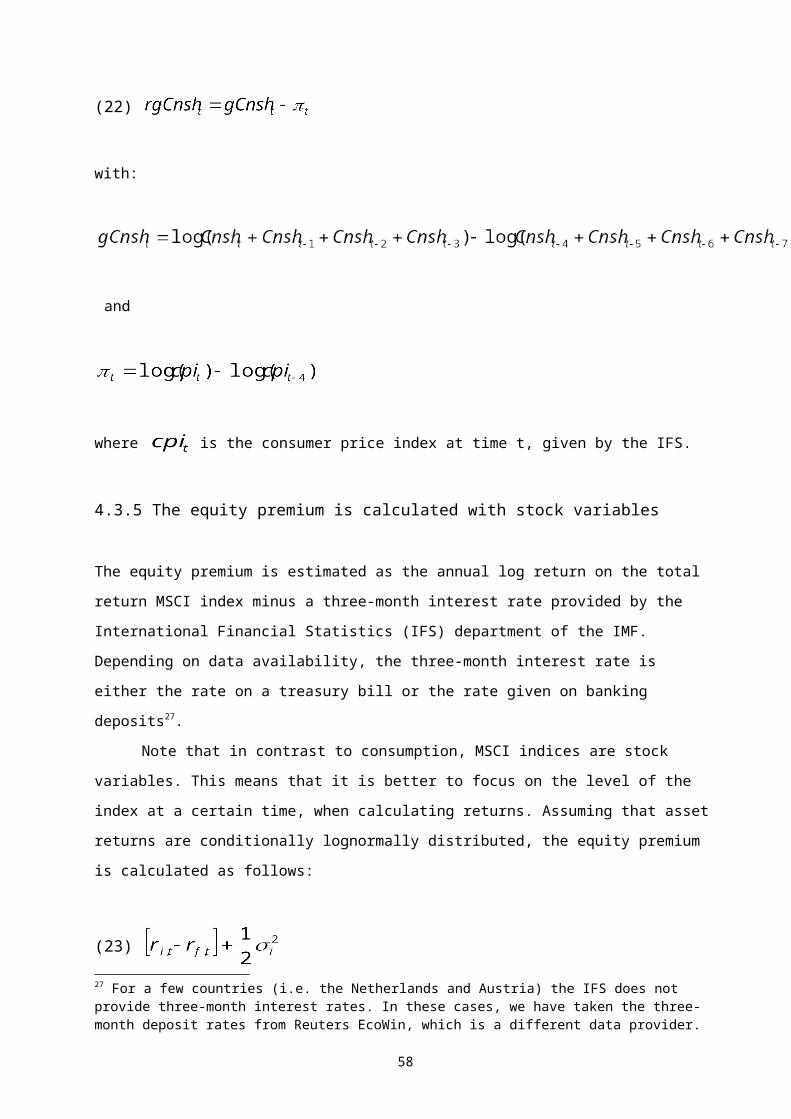
(33)

in which case the share of labor income in total income is calculated as

Table 13 in the National Accounts gives a detailed breakdown of how households and corporations

generate their income and which part of this income flows to the government in the form of tax money. In

essence, the table estimates the amount income that households and corporations have at their disposal.

Box 3 will summarize this process for households38:

Box 3: Table 13 in the National Accounts

Simplified accounts for households and non-profit institutions serving households:

Generation of income account

1) Values added, gross2) -/- Compensation of employees payable3) -/- Taxes on production and imports payable4) +/+ Subsidies on production and imports receivable5) Operating surplus and mixed income, gross6) of which Mixed income, gross

Distribution of income account

7) +/+ Compensation of employees receivable8) +/+ Property income receivable9) -/- Property income payable10) +/+ Social contributions and social benefits, other than social transfers in kind, receivable11) +/+ Other current transfers, receivable12) -/- Current taxes on income, wealth etc., payable13) -/- Social contributions and social benefits, other than social transfers in kind, payable14) -/- Other current transfers, payable15) Disposable income, gross Source: OECD

Finally, for our seven countries, Table 12 gives the average labor income tax ratios:

38 Note, to get net disposable income, gross operating surplus and mixed income should be corrected for depreciations, which can be found in the capital account of Table 13, line 20

58

Table 12: Average effective tax ratios on labor income

  sample period average labor income tax ratio  

United States 1971.4 - 2006.4 21.9United Kingdom 1988.4 - 2005.4 24.3

Canada 1971.4 - 2004.4 26.1Belgium 1996.4 - 2006.4 43.5France 1979.4 - 2007.4 39.8

Netherlands 1990.1 - 2006.4 34.2Austria 1997.4 - 2006.4 42.3

Source: OECD, own calculations

Appendix D: EViews programs

59

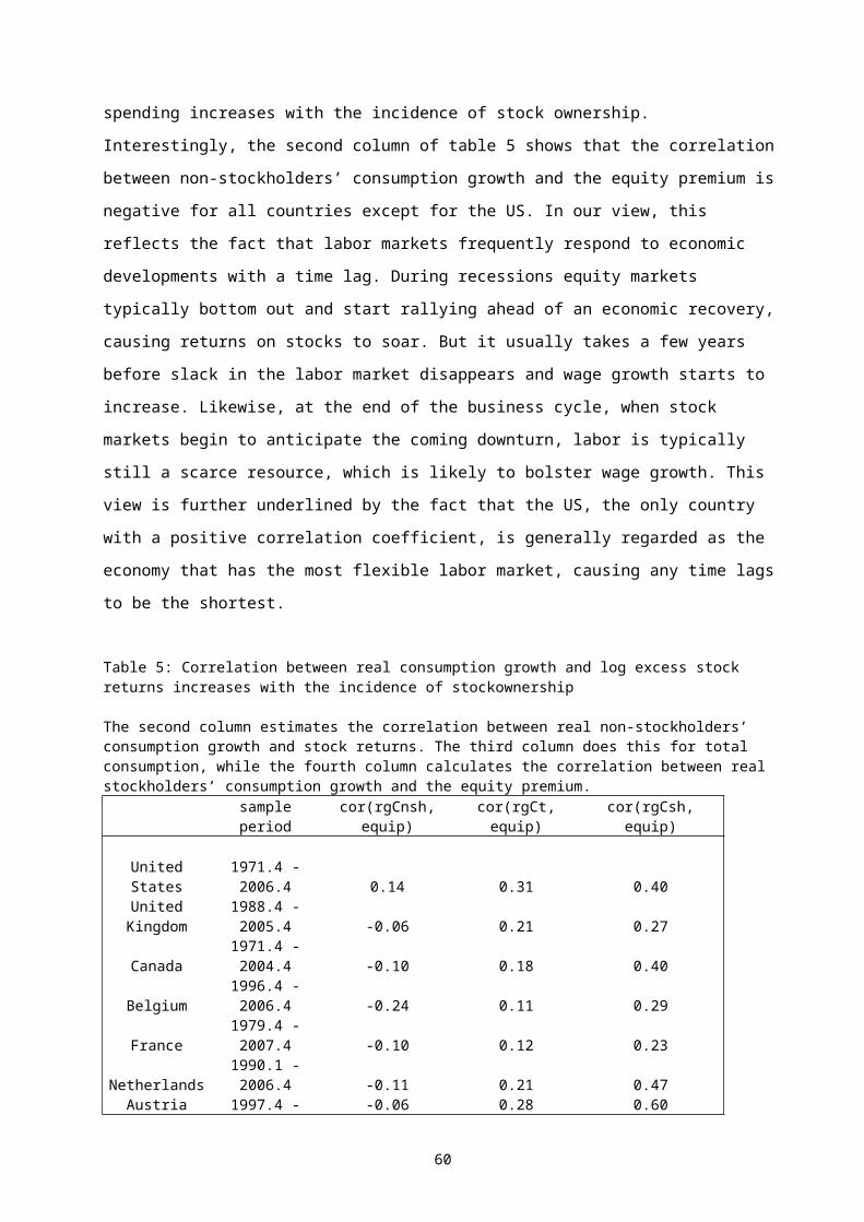
Appendix D gives the EViews programs that have been used for this thesis. The first program has been

used to calculate the average labor income tax ratios, while the second program has been used to estimate

all data that concerns the difference between stockholders’ and non-stockholders’ consumption.

Program: Average labor income tax ratio (social security contributions not deductible)

Program: Average labor income tax ratio (social security contributions deductible)

Program : Risk aversion levels for stockholders and non-stockholders

60

open g:\masterthesis\scriptie\eviewsscriptie2\us2tax

'Meaning of symbols: gmixi = gross mixed income (ospue)'cfc = consumption of fixed capital gopers = gross operating surplus nmixi = net mixed income pei = property income wag = wages comp = compensation

series nmixi = gmixi - (cfc/gopers)*gmixiseries taxratiotot = t1100/(nmixi + pei + wag)

series alpha = wag/(nmixi + pei + wag)

series taxratiolab = ((taxratiotot*wag) + t2100 + t2200 + (alpha*t2400) + t3000)/(comp + t3000)

open g:\masterthesis\scriptie\eviewsscriptie2\belgium2tax

'Meaning of symbols: gmixi = gross mixed income (ospue)'cfc = consumption of fixed capital gopers = gross operating surplus nmixi = net mixed income pei = property income wag = wages comp = compensation

series nmixi = gmixi - (cfc/gopers)*gmixiseries taxratiotot = t1100/(nmixi + pei + wag - t2100 - t2300 - t2400)

series alpha = (wag - t2100)/(nmixi + pei + wag - t2100 - t2300)

series taxratiolab = (taxratiotot * (wag - t2100 - (alpha*t2400)) + t2100 + t2200 + (alpha*t2400) + t3000)/(comp + t3000)

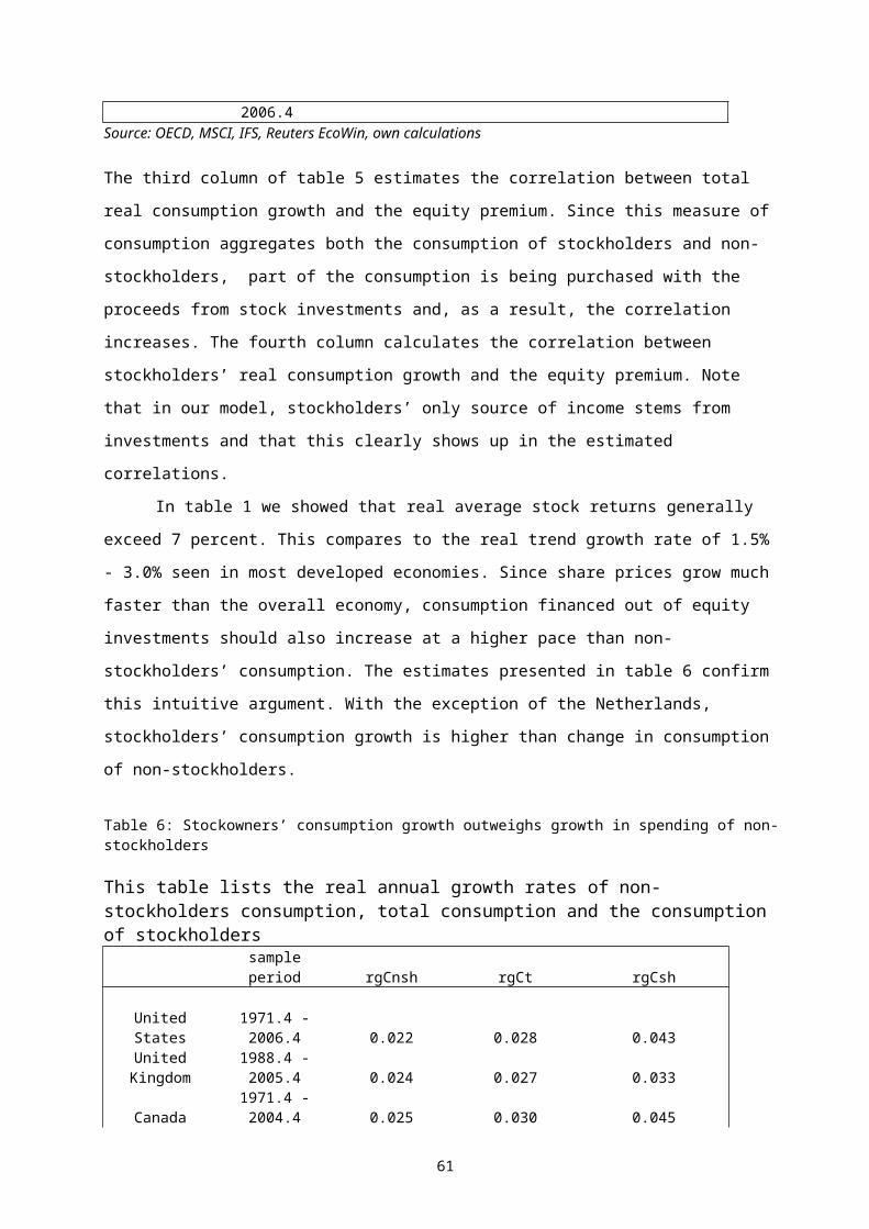
61

open g:\masterthesis\scriptie\eviewsscriptie2\US2'second method look at the annual change, where the change is calculated in the same way as the change in GDP'nominalseries gtcons =log(cons + cons(-1) + cons(-2) + cons(-3)) - log(cons(-4) + cons(-5) + cons(-6) + cons(-7))series kapcons = cons - ((1-taxratiolab)*comp)series gkapcons = log(kapcons + kapcons(-1) + kapcons(-2) + kapcons(-3)) - log(kapcons(-4) + kapcons(-5) +kapcons(-6) +kapcons(-7))series labcons = cons - kapconsseries glabcons = log(labcons + labcons(-1) + labcons(-2) + labcons(-3)) - log(labcons(-4) + labcons(-5) + labcons(-6) +labcons(-7))series gmsci = log(msci) - log(msci(-4))series ttbr = log(1 + (tbr/100))series equip = gmsci - ttbr

'realseries inf = log(cpi) - log(cpi(-4))series rgtcons = gtcons - infseries rgkapcons = gkapcons - infseries rgmsci = gmsci - infseries rtbr = ttbr - infseries rglabcons = glabcons - inf

smpl 1971.1 2006.4scalar sc1 = @mean(equip)scalar sc2 = @var(rgmsci)scalar meaneqp = (sc1 +0.5*sc2)scalar stock = @cov(rgmsci, rgtcons)scalar bond =@cov(rtbr, rgtcons)scalar equi = @cov(equip, rgtcons)scalar r = meaneqp/@cov(equip, rgtcons)scalar rr =meaneqp/@cov(equip, rgkapcons)scalar rl = meaneqp/@cov(equip, rglabcons)scalar cort = @cor(equip, rgtcons)scalar corr = @cor(equip,rgkapcons)scalar corl = @cor(equip, rglabcons)scalar covl =@cov(equip, rglabcons)scalar covt = @cov(equip, rgtcons)scalar covk = @cov(equip, rgkapcons)

scalar a = @mean(rgmsci)scalar t = @mean(taxratiolab)

scalar varlabcon = @var(rglabcons)scalar vartotcons = @var(rgtcons)scalar varcapcons = @var(rgkapcons)

scalar rglacons = @mean(rglabcons) + 0.5*varlabconscalar rgtotcons = @mean(rgtcons) + 0.5*vartotconsscalar rgcapcons = @mean(rgkapcons) + 0.5*varcapconsscalar sdlabcons = @stdev(rglabcons)scalar sdtotcons = @stdev(rgtcons)scalar sdkapcons = @stdev(rgkapcons)equation eq01.ls rgtcons-rglabcons = c(1) + c(2)*equipequation eq02.ls rgkapcons - rgtcons = c(3) + c(4)*equipequation eq03.ls rgkapcons-rglabcons = c(5) + c(6)*equip

Websites:

OECD (general website and data): http://www.oecd.org

OECD (data): http://www.sourceoecd.org

OECD stat: http://stats.oecd.org/WBOS/index.aspx

UN (explanation of National Accounts): http://unstats.un.org/unsd/sna1993/toctop.asp?L1=7

US Bureau of Labor Statistics: http://www.bls.gov

US Bureau of Economic Analysis: http://www.bea.gov

US National Bureau of Economic Research: http://www.nber.org

62

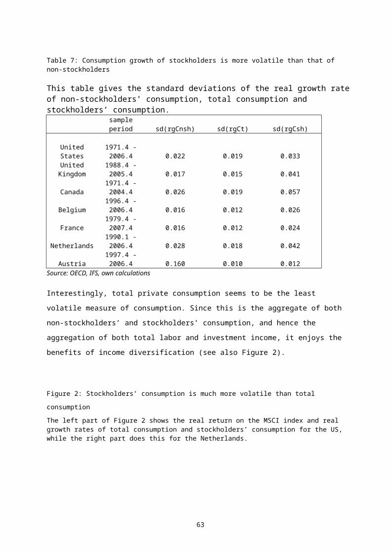
References:

Abel, A.B. Asset Prices under Habit Formation and Catching Up with the Joneses, American Economic

Revies, vol 80, no. 2 (May 1990) 38 - 42

Aiyergari R., Gertler M., Asset Returns with Transaction Costs an Uninsured Individual Risk, Journal of

Monetary Economics 27, (1991), 311 - 331

Aiyergari R., Explaining Financial Market Facts: The Importance of Incomplete Markets and Transaction

Costs, Federal Reserve Bank of Minneapolis, Quarterly Review Vol. 17, (Winter 1993) 17-31

Attanasio O., Banks J., Tanner S., Asset Holding and Consumption Volatility, Journal of Political

Economy (2002) Vol. 110, No. 4

Avery R.B., Elliehausen G.E., Kennickell A.B., Measuring Wealth with Survey Data: An Evaluation of

the 1983 Survey of Consumer Finances, Review of Income and Wealth 34 (December 1988) 339-69

Bansal Ravi, Coleman Wilbur John, A Monetary Explanation of the Equity Premium, Term Premium,

and Risk-Free Rate Puzzles, The Journal of Political Economy, Vol. 104, No. 6 (December 1996), 1135 -

1171

Bernartzi S., Thaler R. H., Myopic Loss Aversion and the Equity Premium Puzzle, The Quarterly journal

of Economics, Vol. 110, No. 1 (Feb. 1995), 73-92

Blanchard, Olivier, Movements in the Equity Premium, Brookings Papers on Economic Activity (1993)

519-43

Brav Alon, Constantinides George M., Geczy Christopher C., Asset Pricing with Heterogeneous

Consumers and Limited Participation: Empirical Evidence, Journal of Political Economy, Vol. 110, No. 4

(2002)

Brown S.J., Goetzmann W.N., Ross S.A., Survival, The Journal of Finance, Vol. 50 No.3 (July 1995)

853-873

Campbell J.Y. Asset Prices, Consumption and the Business Cycle (1998) in J.B. Taylor, M.

Woodford Handbook of Macroeconomics

63

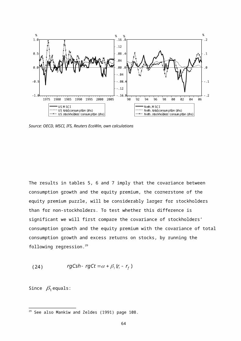
Campbell J.Y., Consumption-Based Asst Pricing, Harvard Institute of Economic Research, Discussion

paper 1974 (2002)

Campbell J.Y., and J.H. Cochrane, By Force of Habit: A Consumption-Based Explanation of Aggregate

Stock Market Behavior, Journal of Political Economy, vol. 107, no. 2, 1995, 202 – 251,

Campbell J.Y., Mankiw N.G., Permanent Income, Current Income, and Consumption, Journal of

Business & Economic Statistics, vol 8, Iss 3, (1990) 293 - 305

Carey D., Rebasona J., Tax Ratios on Labour and Capital Income and on Consumption, OECD Economic

Studies No. 35 2002 129-174

Cheung S.C., Een Macro-Econmische Benadering van de Equity Premium Puzzle: De Heterogeniteit van

Mankiw en Zeldes Herzien, Masterthesis Erasmus University

Constantinides G.M., Intertemporal Asset Pricing with Heterogeneous Consumers and without Demand

Aggregation, Journal of Business, Vol. 55, No. 2, 1982

Constantinides G.M., Habit Formation: A Resolution of the Equity Premium Puzzle, Journal of Political

Economy, vol 98, no.3 (June 1990) 519 - 543

Constantinides George, Duffie Darrel, Asset Pricing With Heterogeneous Consumers, The Journal of

Political Economy, Vol 104, no. 2 (April 1996), 219 - 240

Constantinides George, Donaldson John, Mehra Rajnish, Junior can’t Borrow: A New Perspective on the

Equity Premium Puzzle, Quarterly Journal of Economics, (February 2002)

Epstein G., Zin Stanley, Substitution, Risk Aversion, and the Temporal Behavior of Consumption Growth

and Asset Returns I: A Theoretical Framework, Econometrica, July (1989), Vol 57, 937 - 969

Epstein G., Zin Stanley, Substitution, Risk Aversion, and the Temporal Behavior of Consumption and

Asset Returns, The Journal of Political Economy, Vol 99, No. 2 (April 1991) 263 - 286

Fortis Bank Nederland, Policymakers sow seeds for recovery, International Economic Outlook, 22

December 2008

64

Friend, I and M.E. Blume, The Demand for Risky Assets, American Economic Review 65, (1975), 900 -

922

Glassman, J.K. and Hassett K.A. Dow 36,000: The New Strategy for Profiting from the Coming Rise in

the Stock Market (1999), Times Books

Grossman S.J., Shiller R.J., Consumption Correlatedness and Risk Measurement in Economies with Non-

Traded Assets and Heterogeneous Information, Journal of Financial Economics Vol. 10, (1982) 195 - 210

Haliassos Michael, Carol C. Bertaut, Why Do So Few Hold Stocks, The Economic Journal, Vol. 105, No.

432 (September 1995) 1110 - 1129

Heaton, J., and D.J. Lucas Evaluating the effects of Incomplete Markets on Risk Sharing and Asset

Pricing, Journal of Political Economy, vol. 104, no. 3 (June 1996) 443 - 487

Heaton, J. and Lucas, D. The Importance of Investor Heterogeneity and Financial Market Imperfections

for the Behavior of Asset Prices, Carnegie-Rochester Conference Series on Public Policy, 1995, 1 - 32

Kahneman D, and Tversky A., Prospect Theory: An Analysis of Decision under Risk, Ecconometrica,

Vol.47, (March 1979) 263 - 291

Kandel Shmuel, Robert F. Stambaugh, Expectations and Volatility of Consumption and Asset Returns,

The Review of Financial Studies, Vol. 3, No. 2. 1990, 207 - 232

Kessler D., Wolf E., A Comparative Analysis of Household Wealth patterns in France and the Unites

States, Review of Income and Wealth 37 (September) 249 - 266

Kocherlakota Narayana R., Disentangling the Coefficient of Relative Risk Aversion from the Elasticity of

Intertemporal Substitution: An Irrelevance Result, The Journal of Finance, vol. 45, No. 1 (March 1990),

175 - 190

Kocherlakota Narayana R., The Equity Premium: It’s Still a Puzzle, Journal of Economic Literature,

vol.34, No. 1. (March 1996), 42 - 71

Levy Haim, Thierry Post, Investments, Prentice Hall 2005

65

Li Haitao, Xu Yuewu, Survival Bias and the Equity Premium, The Journal of Finance, Vol 57, No. 5

(October 2002), 1981 - 1995

Mankiw N.G., The Savers Spenders Theory of Fiscal Policy, The American Economic Review, 90 (2000)

120 - 126

Mankiw N.G., Zeldes S.P., The Consumption of Stockholders and Nonstockholders, Journal of Financial

Economics 29 (1991) 97 - 112

McGratten, E.R., and E.C. Prescott, Taxes, Regulations, and Asset Prices, Working Paper No. 610,

Federal Reserve Bank of Minneapolis

Mehra R., Prescott E.C., The Equity Premium Puzzle, Journal of Monetary Economics 15 (1985) 145 -

161

Mehra R., Prescott E.C., The Equity Risk Premium: A Solution?, Journal of Monetary Economics No.22

(1988) 133 - 136

Mehra R., The Equity Premium: Why is it a Puzzle?, Financial Analyst Journal, February (2003)

Nakamoto M., Lindsay W., Japanese Retail Investors return home, Financial Times, June 23 2009

OECD, Quarterly National Accounts: Sources and Methods Used by OECD Countries

OECD, National Accounts of OECD Countries, Volume II a, 1995-2006 Detailed Tables

OECD, Taxing Wages: 2003/2004

OECD, Taxing Wages: 2006/2007

OECD, Revenue Statistics 1965 – 2006, 2007

Post G.T., van den Assem M.J., Miljoenenjacht:, voer voor economen, Economische Statistische

Berichten, (december 2005)

Rietz T.A., The Equity Risk Premium: A Solution, Journal of Monetary Economics 22 (1988) 117 - 131

66

UN 1993 SNA- Table of Contents, Explanation of National Accounts

Vissing-Jørgensen Annette, Limited Asset Market Participation and the Elasticity of Intertemporal

Substitution, Journal of Political Economy Vol. 110 No. 4 (2002)

Weil Philippe, The Equity Premium Puzzle and the Risk-Free Rate Puzzle, Journal of Monetary

Economics 24 (1989) 401 - 421

Wolf Edward N., Recent Trends in the Size Distribution of Household Wealth, Journal of Economic

Perspectives 12 (1998) 131 - 150

Wolf Edward N, Recent Trends in Wealth Ownership 1983 - 1998, Jerome Levy Economics Institute,

Working Paper No. 300, (April 2000)

67

68