IMPLEMENTATION OF A β-NQR SYSTEM AT THE NSCL FOR

GROUND STATE QUADRUPOLE MOMENT

MEASUREMENTS

By

Rankothge R. Weerasiri

A THESIS

Submitted toMichigan State University

in partial fulfillment of the requirementsfor the degree of

MASTER OF SCIENCE

Department of Chemistry

2007

ABSTRACT

IMPLEMENTATION OF A β-NQR SYSTEM AT THE NSCL FOR GROUNDSTATE QUADRUPOLE MOMENT MEASUREMENTS

By

Rankothge R. Weerasiri

The nuclear electric quadrupole moment, Q, is a direct measure of the nuclear

charge distribution, and provides an important test of nuclear structure models. The

β detected nuclear quadrupole resonance (β-NQR) method is a technique to measure

ground state Q of unstable nuclei.

A β-NQR system has been constructed at the NSCL. Several challenges had to be

overcome to build the β-NQR system, including the implementation of multi-radio

frequencies, high rf magnetic field strength, short rf application time due to the short

half-life of exotic nuclei of interest. The new system has four function generators to

produce the required rf signals for I ≤ 2 nuclei. The rf signals are amplified to a

maximum of 250 W. After the amplifier, a switched LCR system is used to maximize

power delivered to the rf coil. Six variable capacitors, a 50 Ω resistor or impedance

matching transformer, and an rf coil represent the complete LCR circuit.

An rf leak test performed on the constructed system showed no significant rf leak-

age from the high voltage rf box, which holds the resistor, transformer, and variable

capacitors. Rf magnetic field strengths were measured to be 18.2 G and 17.6 G for

frequencies of 700±10 kHz and 1200±10 kHz, respectively, at maximum power.

First application of the new β-NQR system will be a precision measurement of the

Q of 37K. A value 114.7±38.2 mb has been reported in the literature, and a new value

with reduced error is important to test the predictions of sd shell model calculations.

The Q of 35K will be measured to find evidence for influence of weak proton binding

energy in the Q of this very neutron-deficient nucleus.

To

my mother, my family,

all my teachers

and friends

iii

ACKNOWLEDGMENTS

I am very grateful to my advisor, Professor Paul F. Mantica, for giving me the

opportunity to come to USA and to study at the MSU/NSCL, for his kind and patient

supervision, valuable guidance and encouragement during the total time period.

I wish to express my sincere gratitude to Dr. Kei Minamisono, who gave many

helpful advice and useful suggestions to fulfill the project successfully.

I thank my guidance committee including Professor Dave Morrissey, Professor

Hendrik Schatz and Professor B. Alex Brown for their valuable guidance.

I like to thanks all of my teachers in the Department of Chemistry / MSU and at

the NSCL

I would like to acknowledge my thanks to all the present and past members of

the beta group at the NSCL including Dr. J. Pereira, Dr. T. J. Mertzimekis, S. N.

Liddick, A. D. Davis, B. E. Tomlin, J. Stoker and J. Pinter who gave lot of help and

a friendly environment to work.

I also like to thank all the members of Professor Dave Morrissey’s group including

Chandana Sumiththrarachchi who let me to stay in his home when I first came here.

My sincere thanks to all the staff of the NSCL, especially the design group and

the electronic group.

Finally, I like to thank Professor Rohini Hewamanna and Professor Pali Ma-

hawatte, University of Colombo, Sri Lanka, who encouraged me to study further.

iv

Contents

1 Introduction 11.1 The nuclear electric quadrupole moment . . . . . . . . . . . . . . . . 11.2 Importance of the quadrupole moment measurements . . . . . . . . . 21.3 The quadrupole moment measuring techniques . . . . . . . . . . . . . 4

2 β-NQR Methodology 72.1 Spin polarization . . . . . . . . . . . . . . . . . . . . . . . . . . . . . 72.2 Implantation of nuclei and preservation of polarization in a host crystal 132.3 Hyperfine interactions . . . . . . . . . . . . . . . . . . . . . . . . . . 132.4 NMR search through β-ray asymmetric angular distribution . . . . . 16

2.4.1 β-ray asymmetric angular distribution . . . . . . . . . . . . . 162.4.2 Manipulation of spin polarization . . . . . . . . . . . . . . . . 182.4.3 Depolarization technique . . . . . . . . . . . . . . . . . . . . . 192.4.4 Adiabatic fast passage (AFP) technique . . . . . . . . . . . . 192.4.5 Extraction of quadrupole moment . . . . . . . . . . . . . . . . 21

3 β-NQR Equipment Implementation 253.1 Radio frequency generation . . . . . . . . . . . . . . . . . . . . . . . 273.2 RF amplification . . . . . . . . . . . . . . . . . . . . . . . . . . . . . 303.3 LCR circuitry . . . . . . . . . . . . . . . . . . . . . . . . . . . . . . . 313.4 Rf coil . . . . . . . . . . . . . . . . . . . . . . . . . . . . . . . . . . . 333.5 Stepper motor controlling system . . . . . . . . . . . . . . . . . . . . 373.6 Vacuum relay switching . . . . . . . . . . . . . . . . . . . . . . . . . 383.7 RPV071 module . . . . . . . . . . . . . . . . . . . . . . . . . . . . . . 44

4 β-NQR system tests 484.1 Calibrating of stepper motor controllers for variable capacitor operation 484.2 Testing the whole system . . . . . . . . . . . . . . . . . . . . . . . . . 49

4.2.1 RF leakage test . . . . . . . . . . . . . . . . . . . . . . . . . . 494.2.2 Cold switching confirmation . . . . . . . . . . . . . . . . . . . 494.2.3 Low power test . . . . . . . . . . . . . . . . . . . . . . . . . . 514.2.4 Maximum rf field test . . . . . . . . . . . . . . . . . . . . . . 524.2.5 Capacitance limits on LCR circuit . . . . . . . . . . . . . . . . 53

v

5 β-NQR Application to 35,37K 545.1 Quadrupole moments of the nuclei in sd shell . . . . . . . . . . . . . 545.2 Quadrupole moments of potassium isotopes . . . . . . . . . . . . . . 555.3 Quadrupole moment measurement of 37K . . . . . . . . . . . . . . . 565.4 Quadrupole moment measurement of 35K . . . . . . . . . . . . . . . 585.5 Experimental details . . . . . . . . . . . . . . . . . . . . . . . . . . . 59

6 Summary 62

Bibliography 65

vi

List of Figures

1.1 Prolate and oblate shapes of nuclear charge distribution . . . . . . . 2

2.1 The momentum transfer in a fragmentation reaction. . . . . . . . . . 9

2.2 Schematic representation of yield and polarization curves of fragmen-tation reaction. . . . . . . . . . . . . . . . . . . . . . . . . . . . . . . 10

2.3 The momentum transfer in a pick-up reaction. . . . . . . . . . . . . . 11

2.4 a). Polarization of 37K in KBr and b). 37K ion yield as functions ofrelative momentum in the proton pick-up reaction. . . . . . . . . . . 12

2.5 Energy levels of I=3/2 nuclei under magnetic field and magnetic field+ electric field gradient. . . . . . . . . . . . . . . . . . . . . . . . . . 14

2.6 Definition of the Euler angles for description of the principal axis ofthe electric field gradient. . . . . . . . . . . . . . . . . . . . . . . . . 17

2.7 Angular distribution of β particles from polarized nuclei. . . . . . . . 18

2.8 The motion of nuclear spin under strong static magnetic field and ro-tating magnetic field . . . . . . . . . . . . . . . . . . . . . . . . . . . 20

2.9 Spin inversion in AFP technique . . . . . . . . . . . . . . . . . . . . . 22

2.10 a) Three frequency sets corresponding to different values of quadrupolecoupling constant for a I = 3/2 nuclei b) Double ratio vs couplingconstant . . . . . . . . . . . . . . . . . . . . . . . . . . . . . . . . . . 24

3.1 Schematic representation of the overall β-NQR system . . . . . . . . 26

3.2 3D drawing of the rf box . . . . . . . . . . . . . . . . . . . . . . . . . 28

3.3 Schematic representation of the radio frequency generating system. . 29

3.4 Schematic representation of dips in the LCR resonance curve becauseof gain reduction feature of the rf amplifier. . . . . . . . . . . . . . . 31

3.5 Schematic representation of a the LCR circuit . . . . . . . . . . . . . 32

vii

3.6 3D drawing of the of the rf coil bobbin and the schematic representationof the orientation of the coil bobbin . . . . . . . . . . . . . . . . . . . 34

3.7 Inductance of rf coil vs turn number. . . . . . . . . . . . . . . . . . . 36

3.8 Schematic representation of the circuit used to measure the DC char-acter of the rf coil. . . . . . . . . . . . . . . . . . . . . . . . . . . . . 36

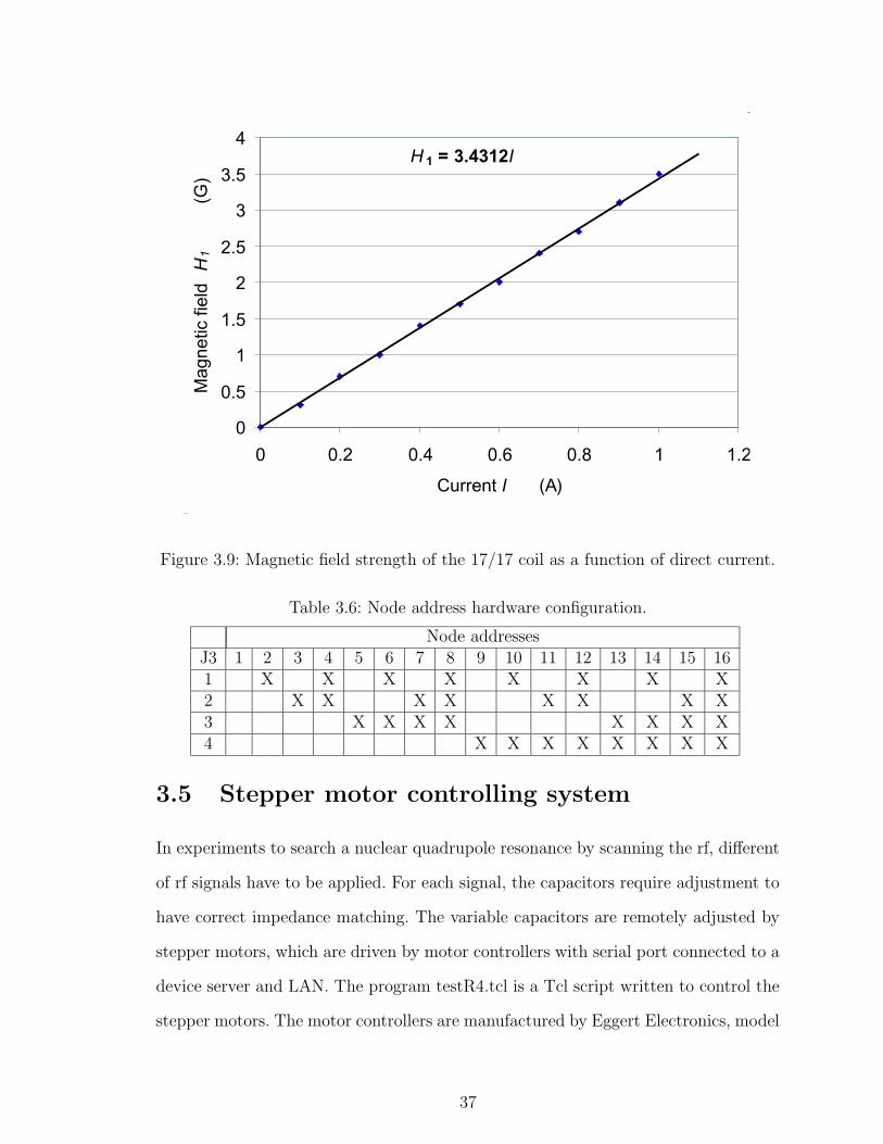
3.9 Magnetic field strength of the 17/17 coil as a function of direct current. 37

3.10 Schematic representation of stepper motor controlling system . . . . . 39

3.11 Schematic representation of power supply for motor controllers. . . . 40

3.12 Schematic representation of switch time measuring circuit. . . . . . . 40

3.13 Relay switch response time. . . . . . . . . . . . . . . . . . . . . . . . 41

3.14 Circuit diagram of relay switch controllers . . . . . . . . . . . . . . . 43

3.15 Relay switch control and rf gate signals . . . . . . . . . . . . . . . . . 43

3.16 Schematic representation of triggering and timing system . . . . . . . 44

3.17 Schematic representation of writing a program to the memory of RPV071. 45

3.18 Schematic representation of a timing program of pulsed-beam depolar-ization method for I=3/2 nuclei . . . . . . . . . . . . . . . . . . . . . 46

3.19 Schematic representation of timing programs of continuous beam de-polarization technique and AFP technique for I=3/2 nuclei . . . . . . 47

4.1 Switch control signal and rf signal. . . . . . . . . . . . . . . . . . . . 50

4.2 LCR resonance frequencies at low power test. . . . . . . . . . . . . . 51

4.3 The circuit for the power tests. . . . . . . . . . . . . . . . . . . . . . 52

5.1 Quadrupole moments of T=1/2 nuclei in the sd shell. . . . . . . . . . 55

5.2 Quadrupole moments of potassium isotopes. . . . . . . . . . . . . . . 56

5.3 Partial decay scheme of 37K. . . . . . . . . . . . . . . . . . . . . . . . 57

5.4 Transition frequencies for the quadrupole moment of 37K . . . . . . . 57

5.5 Decay scheme of 35K. . . . . . . . . . . . . . . . . . . . . . . . . . . . 59

5.6 Transition frequencies of 35K . . . . . . . . . . . . . . . . . . . . . . 60

5.7 β-NMR setup at NSCL . . . . . . . . . . . . . . . . . . . . . . . . . . 61

viii

List of Tables

3.1 Available function generators. . . . . . . . . . . . . . . . . . . . . . . 30

3.2 Technical details of the RF amplifier. . . . . . . . . . . . . . . . . . . 31

3.3 Technical details of the vacuum variable capacitors. . . . . . . . . . . 32

3.4 Variation of inductance with turn number of rf coils. . . . . . . . . . 35

3.5 Variation of magnetic field strength of the rf coil (17/17) with current. 35

3.6 Node address hardware configuration. . . . . . . . . . . . . . . . . . . 37

3.7 Specifications of relay switches. . . . . . . . . . . . . . . . . . . . . . 38

3.8 Switch response time of relay switches. . . . . . . . . . . . . . . . . . 41

4.1 Upper and lower limits for stepper motors. . . . . . . . . . . . . . . . 49

4.2 Results of the rf leakage test. . . . . . . . . . . . . . . . . . . . . . . 50

4.3 High power tests of the whole system. . . . . . . . . . . . . . . . . . . 53

ix

Chapter 1

Introduction

1.1 The nuclear electric quadrupole moment

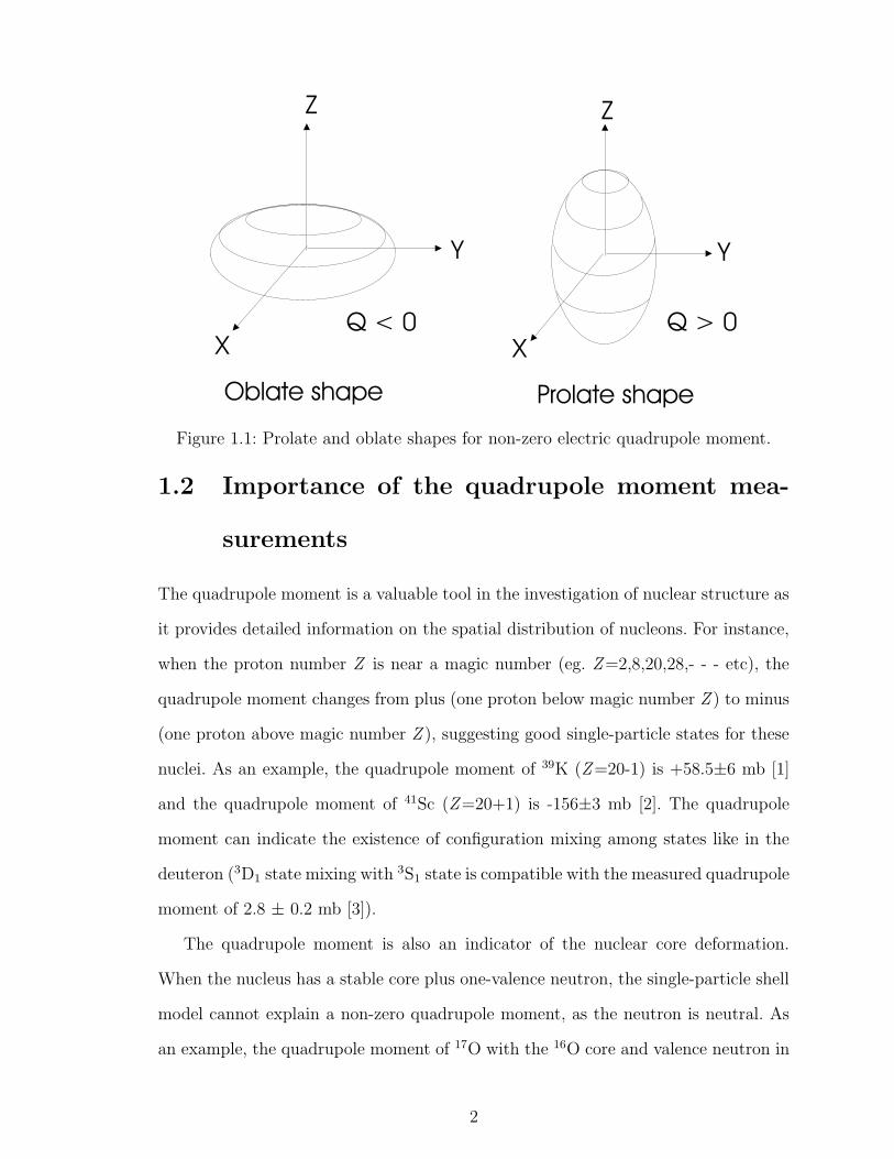
The nuclear electric quadrupole moment is a quantity that describes the shape of

the nuclear charge distribution. A quadrupole moment of zero indicates a spherically

symmetric charge distribution. By convention, the value of the quadrupole moment

is taken to be positive for a prolate-shaped charge distribution and negative for an

oblate-shaped charge distribution, as shown in Figure 1.1. The electric quadrupole

moment operator is given as,

eQ =

∫

ρ(~r)r2(3cos2θ − 1)dv, (1.1)

where eQ is the quadrupole moment, ρ(~r) is the charge density, ~r - (r, θ, φ) in polar

coordinates and dv is the small volume at point r.

1

Oblate shape Prolate shape

Z Z

Y

X

Y

XQ < 0 Q > 0

Figure 1.1: Prolate and oblate shapes for non-zero electric quadrupole moment.

1.2 Importance of the quadrupole moment mea-

surements

The quadrupole moment is a valuable tool in the investigation of nuclear structure as

it provides detailed information on the spatial distribution of nucleons. For instance,

when the proton number Z is near a magic number (eg. Z=2,8,20,28,- - - etc), the

quadrupole moment changes from plus (one proton below magic number Z ) to minus

(one proton above magic number Z ), suggesting good single-particle states for these

nuclei. As an example, the quadrupole moment of 39K (Z=20-1) is +58.5±6 mb [1]

and the quadrupole moment of 41Sc (Z=20+1) is -156±3 mb [2]. The quadrupole

moment can indicate the existence of configuration mixing among states like in the

deuteron (3D1 state mixing with 3S1 state is compatible with the measured quadrupole

moment of 2.8 ± 0.2 mb [3]).

The quadrupole moment is also an indicator of the nuclear core deformation.

When the nucleus has a stable core plus one-valence neutron, the single-particle shell

model cannot explain a non-zero quadrupole moment, as the neutron is neutral. As

an example, the quadrupole moment of 17O with the 16O core and valence neutron in

2

the 1d5/2 shell, is -25.78 mb [4]. The presence of a quadrupole moment of 17O can be

explained by the core deformation induced by the valence neutron. In the higher-mass

region, large quadrupole moments are observed that are several times larger than the

single-particle shell model predictions. As an example, the quadrupole moment of

20483 Bi is -700 ± 200 mb [2], which contains an even number of neutrons and one odd

proton outside the shell closure at Z=82. The calculated quadrupole moment using

single-particle shell model equations [5],

Qint = − < r2 >[2J − 1

2J + 2

]

, (1.2)

Qsp = Qint

[ J(2J − 1)

(J + 1)(2J + 3)

]

, (1.3)

is 246.4 mb. In equation 1.2 and 1.3, Qint is the intrinsic quadrupole moment, Qsp

is the spectroscopic quadrupole moment, r is the nuclear radius and J is the nuclear

spin. The intrinsic quadrupole moment is the quadrupole moment of a deformed nu-

cleus whose orientation is fixed in space. However, quantum-mechanically, a deformed

nucleus and its orientation are described by a wave function. In a β-NQR experiment,

we can measure only the projection of the intrinsic quadrupole moment to the ref-

erence axis that is called the spectroscopic quadrupole moment. The enhancement

of the experimental quadrupole moment implies large core deformation due to the

collective effect of nucleons. The nucleons in the unfilled shells move in a net nuclear

potential produced by the core. This potential is not the spherically symmetric one of

the shell model, but undergoes deformation. Therefore, even in the ground state, the

core is affected by the nucleons in the unfilled shell because of their non-spherically

symmetry.

The shape of the nucleus is one of the most important properties in understanding

nuclear structure far from the stability line. From the experiments of the interaction

cross-section measurements, nuclear matter radii can be determined. However, the

nuclear charge radius of 8B determined by the β-NQR measurement is 20% larger

3

than the matter radius of 2.45 fm determined from the interaction cross-section mea-

surement [6]. Moreover, the measured quadrupole moment of 8B by β-NQR method

is twice as large as the theoretical value predicted by conventional shell model calcu-

lations. This may be a result of the presence of proton halo due to the small proton

separation energy (140 keV) as claimed by T. Minamisono et al. [6]. However, the

Coulomb force among the protons, in opposition to the nuclear force, may prevent

the growth of the halo structure and push the protons inside the Coulomb barrier. In

addition, the last valence proton of 8B lies in a 1p3/2 state and the centrifugal barrier

is also against the formation of proton halo. M. Fukuda et al. measured the matter

radius of 8B using cross section measurements at projectile energies of 40 MeV/A and

60 MeV/A and proved that it is comparable with the charge radius extracted from

the β-NQR measurement [7]. This proves that β-NQR technique could be used as a

tool to measure the radial extent of the nuclei.

1.3 The quadrupole moment measuring techniques

The ground state quadrupole moment of exotic nuclei can be obtained using several

different techniques. As an example, the quadrupole moment can be deduced from the

reduced transition probabilities, B(E2). For even-even nuclei, rotational energy levels

are much simpler than in odd-even or odd-odd nuclei. Therefore, even-even nuclei

are preferentially used to extract B(E2) values and to deduce the intrinsic quadru-

pole moment. However, the B(E2) connects two states and extraction of quadrupole

moment of a respective state is theory dependent.

Laser spectroscopy is another technique used to measure the quadrupole moment

that involves hyperfine interactions of atoms. A laser beam induces transitions among

hyperfine levels, which are a result of coupling of electron spin with nuclear spin. The

hyperfine magnetic coupling constant (A) and hyperfine quadrupole coupling constant

(B), deduced from the resonance laser frequencies, can be used to deduce the magnetic

4

moment and the quadrupole moment. Restrictions in the laser spectroscopy technique

include the desired simple electronic structure of the system and limited available laser

frequencies.

Microwave spectroscopy can be applied to measure the quadrupole moment of

gas phase molecules. This technique is closely related to laser spectroscopy hyperfine

structure measurements. The intensity of the molecular beam should be at least 1017

pps to have a good accuracy [8]. Far from the stability line, the production rates of

isotopes are well below this limiting value.

Low temperature nuclear orientation is another method to determine the ground

state quadrupole moment. Lowering the temperature to the milliKlevin range induces

nuclear polarization, from which the quadrupole moment could be extracted from the

anisotropic distribution of γ and β rays. In general, the lifetime of the nuclei under

investigation should be may minutes or longer, due to the time required to orient the

nuclear spin ensemble. For the study of exotic nuclei, lifetimes are typically in the

millisecond range.

The method that will be discussed in this thesis is the Beta Nuclear Quadrupole

Resonance β-NQR method. It has several advantages over the above-mentioned tech-

niques. In contrast to B(E2) measurements, the β-NQR technique is capable to mea-

sure the ground state quadrupole moments of odd-even or odd-odd nuclei with theory

independent way. The β-NQR method uses a strong magnetic field that de-couples the

electron and nuclear spin that excludes the requirement of simple electronic structure

in laser spectroscopy. The β-NQR technique is sensitive to the beam intensities even

around 101 pps that is about 16 orders of magnitude lower than in microwave spec-

troscopy. This technique is capable to cope with nuclei having lifetimes as low as 10

ms that is much shorter than the requirement in low temperature nuclear orientation

technique.

In addition to the advantages stated above, implementation of β-NQR method at

the NSCL is desirable, because the NSCL facility is capable of producing spin po-

5

larized β emitting nuclei far from the stability line. Low production rates and short

lifetimes are the major limitations in the quadrupole moment measurements. The β-

NQR technique is one of the best methods to measure quadrupole moment detecting

spin polarization by β-ray asymmetry even with those limitations. Another advan-

tage is that it is implemented as an improvement of the present β-NMR system that

has successfully measured spin polarization by β-ray asymmetry in several previous

experiments. The β-NQR is a technique to measure nuclear electric quadrupole mo-

ment of unstable nuclei taking advantage of β-ray asymmetric distribution from spin

polarized-nuclei and a detailed explanation is given in chapter 2.

6

Chapter 2

β-NQR Methodology

The β-ray detected Nuclear Quadrupole Resonance (β-NQR) is a technique to mea-

sure nuclear electric quadrupole moments of unstable nuclei taking advantage of the

β-ray asymmetric-angular distribution from spin-polarized nuclei. The β-NQR tech-

nique has four principle requirements.

1. Nuclear ensemble must be polarized.

2. Polarization must be maintained for the nuclear lifetime.

3. There must be electric quadrupole interactions to observe the quadrupole mo-

ment.

4. Destruction of polarization by applied radio frequency (rf) magnetic field.

Each requirement will be explained in detail in the following sections.

2.1 Spin polarization

The nuclear spin polarization is one of the major requirements of the β-NQR tech-

nique. The nuclear spin is a result of the coupling of intrinsic spin of the nucleons

to the orbital angular momentum of nucleons. The nuclear spins are, in general, ran-

domly oriented. Therefore a sample of nuclei has zero net spin orientation. However,

if the nuclear spins are preferentially oriented relative to some external reference, the

7

nuclei are said to be spin polarized. In quantum mechanics, the spin polarization can

be considered as a linear distribution of population in magnetic sub-states given by

equation,

P = Σmam/I, (2.1)

where P is the nuclear polarization, m is the magnetic quantum number, am is the

population of magnetic sub-state m and I is the nuclear spin.

Low temperature nuclear orientation, laser optical pumping, nuclear reactions,

etc., can generate polarization. In this thesis, production of polarization by intermediate-

energy nuclear reactions is considered. In projectile fragmentation, nucleons in the

overlap region of the target and the projectile are removed and the remaining part of

the projectile moves as the projectile-like fragment with almost the same velocity of

the incident projectile. In this process, which is essentially peripheral, momentum is

carried away by the removed part and as a result the projectile-like fragment gains

an angular momentum L, which leads to the spin polarization of the projectile-like

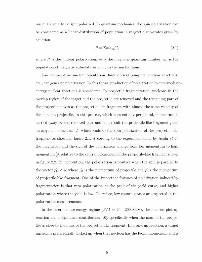
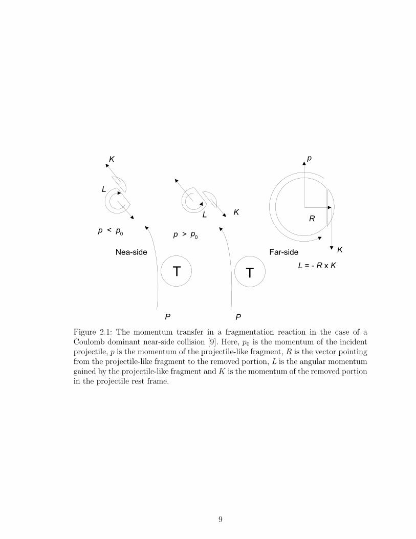
fragment as shown in figure 2.1. According to the experiment done by Asahi et al,

the magnitude and the sign of the polarization change from low momentum to high

momentum [9] relative to the central momentum of the projectile-like fragment shown

in figure 2.2. By convention, the polarization is positive when the spin is parallel to

the vector ~p0 × ~p, where ~p0 is the momentum of projectile and ~p is the momentum

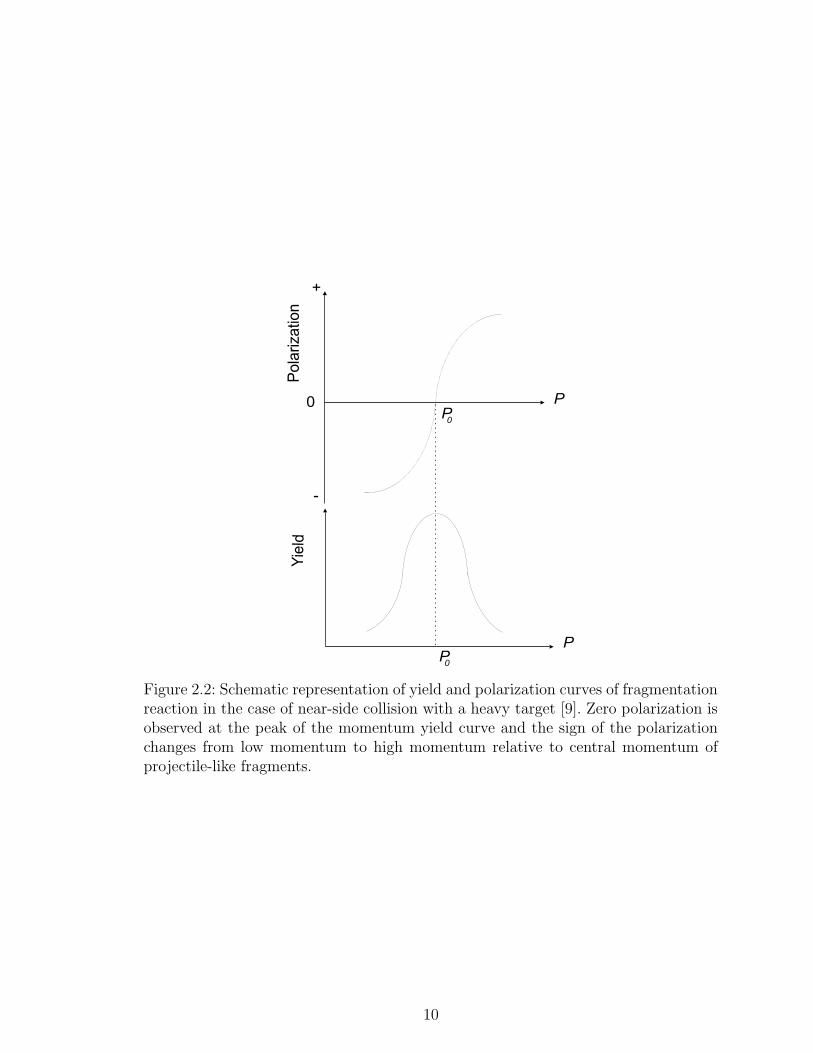
of projectile-like fragment. One of the important features of polarization induced by

fragmentation is that zero polarization at the peak of the yield curve, and higher

polarization where the yield is low. Therefore, low counting rates are expected in the

polarization measurements.

In the intermediate-energy regime (E/A = 20 - 200 MeV), the nucleon pick-up

reaction has a significant contribution [10], specifically when the mass of the projec-

tile is close to the mass of the projectile-like fragment. In a pick-up reaction, a target

nucleon is preferentially picked up when that nucleon has the Fermi momentum and is

8

T

K

p < p0

T

K

p > p0

L R K= - x

R

p

K

P P

L

L

Nea-side Far-side

Figure 2.1: The momentum transfer in a fragmentation reaction in the case of aCoulomb dominant near-side collision [9]. Here, p0 is the momentum of the incidentprojectile, p is the momentum of the projectile-like fragment, R is the vector pointingfrom the projectile-like fragment to the removed portion, L is the angular momentumgained by the projectile-like fragment and K is the momentum of the removed portionin the projectile rest frame.

9

0

+

-

P

P0

P

P0

Pola

rization

Yie

ld

Figure 2.2: Schematic representation of yield and polarization curves of fragmentationreaction in the case of near-side collision with a heavy target [9]. Zero polarization isobserved at the peak of the momentum yield curve and the sign of the polarizationchanges from low momentum to high momentum relative to central momentum ofprojectile-like fragments.

10

p

K

R

L R K= x

TargetProjectile

0

p

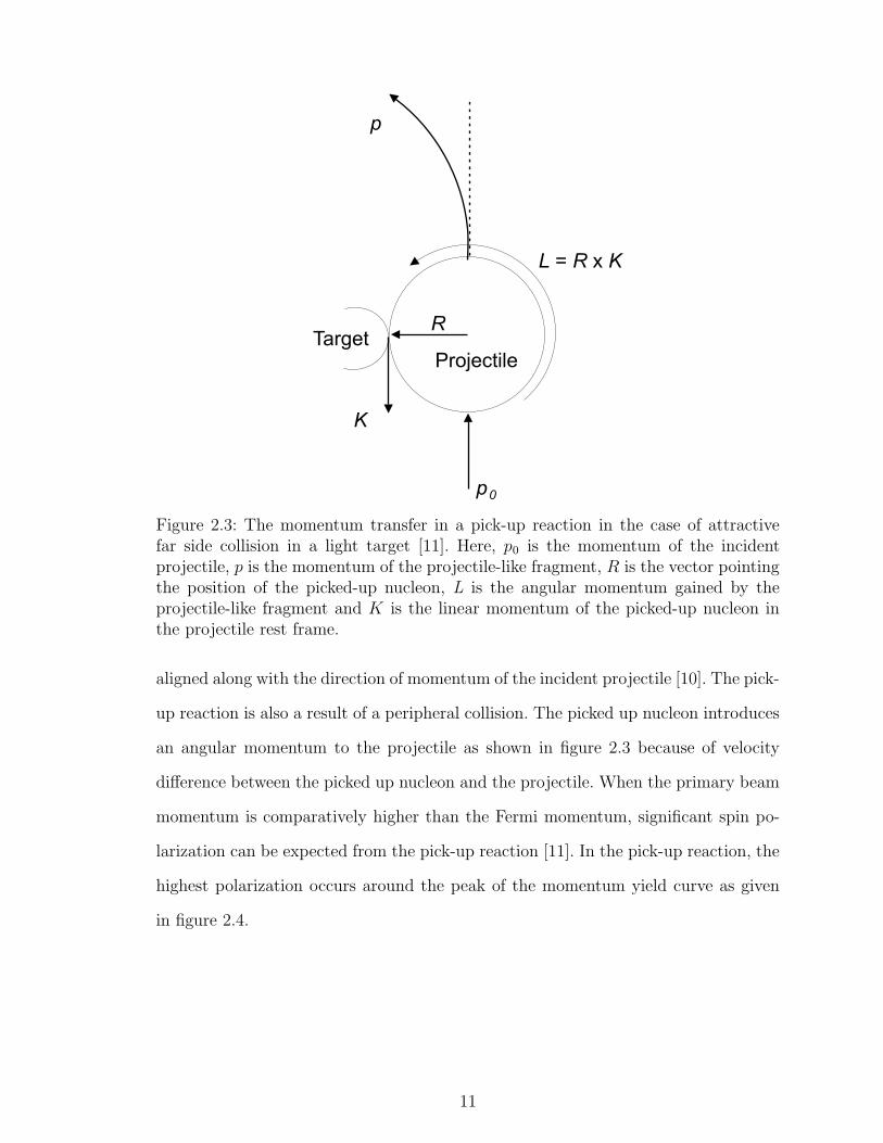
Figure 2.3: The momentum transfer in a pick-up reaction in the case of attractivefar side collision in a light target [11]. Here, p0 is the momentum of the incidentprojectile, p is the momentum of the projectile-like fragment, R is the vector pointingthe position of the picked-up nucleon, L is the angular momentum gained by theprojectile-like fragment and K is the linear momentum of the picked-up nucleon inthe projectile rest frame.

aligned along with the direction of momentum of the incident projectile [10]. The pick-

up reaction is also a result of a peripheral collision. The picked up nucleon introduces

an angular momentum to the projectile as shown in figure 2.3 because of velocity

difference between the picked up nucleon and the projectile. When the primary beam

momentum is comparatively higher than the Fermi momentum, significant spin po-

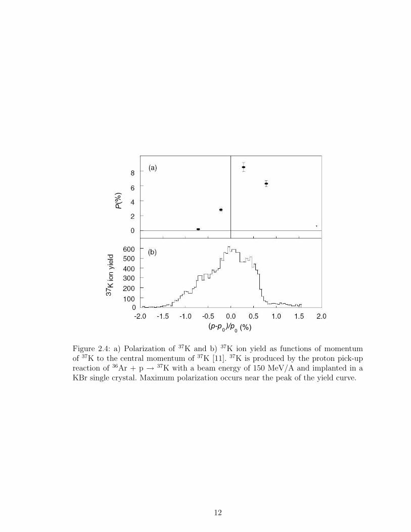
larization can be expected from the pick-up reaction [11]. In the pick-up reaction, the

highest polarization occurs around the peak of the momentum yield curve as given

in figure 2.4.

11

(p-p )/p0 0

(%)

P(%

)

Figure 2.4: a) Polarization of 37K and b) 37K ion yield as functions of momentumof 37K to the central momentum of 37K [11]. 37K is produced by the proton pick-upreaction of 36Ar + p → 37K with a beam energy of 150 MeV/A and implanted in aKBr single crystal. Maximum polarization occurs near the peak of the yield curve.

12

2.2 Implantation of nuclei and preservation of po-

larization in a host crystal

Polarized nuclei are implanted in a host crystal, which has an electric field gradient.

In the β-NQR technique, the polarization is measured by the angular distribution

of β particles. Therefore, polarization has to be preserved until the β decay occurs.

Depolarization occurs due to two main processes: spin-lattice relaxation and spin-spin

relaxation. Spin-lattice relaxation or longitudinal relaxation is a result of interaction

between nuclear spin with the surrounding crystal lattice that is characterized by the

spin-lattice relaxation time T1. In the process of spin-spin relaxation, or transverse

relaxation, polarization is destroyed due to the interaction between opposite spins.

This process is characterized by spin-spin relaxation time T2. The spin polarization

is preserved with the help of a strong external magnetic field H0 and symmetric

environment in the crystal. In addition, the strong magnetic field is helpful to avoid the

possible reduction of the polarization through coupling between the nucleus and the

orbital electrons during its flight from the final degrader to the host crystal. The strong

magnetic field prevents the coupling of the nuclear moments with the fluctuating

electromagnetic fields produced by the radiation damages during the implantation

process into the crystal.

2.3 Hyperfine interactions

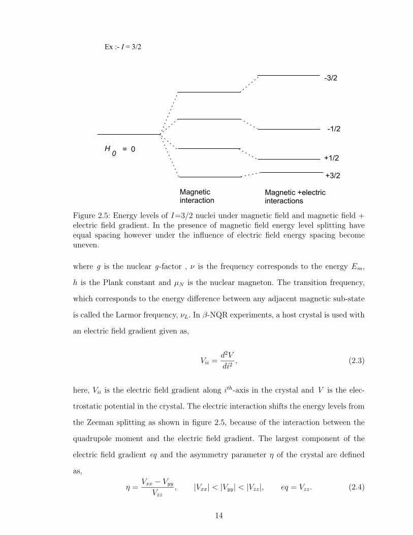
In the presence of a strong magnetic field H0, a nuclear spin energy level breaks

degeneracy into several magnetic sub-states (Zeeman splitting) represented by the

magnetic quantum number as shown in figure 2.5. The energy of the magnetic state,

Em, is given as,

Em = −mgµNH0 = hν, (2.2)

13

Ex :- = 3/2I

H0

= 0

Magneticinteraction

Magnetic +electricinteractions

-3/2

-1/2

+1/2

+3/2

Figure 2.5: Energy levels of I=3/2 nuclei under magnetic field and magnetic field +electric field gradient. In the presence of magnetic field energy level splitting haveequal spacing however under the influence of electric field energy spacing becomeuneven.

where g is the nuclear g-factor , ν is the frequency corresponds to the energy Em,

h is the Plank constant and µN is the nuclear magneton. The transition frequency,

which corresponds to the energy difference between any adjacent magnetic sub-state

is called the Larmor frequency, νL. In β-NQR experiments, a host crystal is used with

an electric field gradient given as,

Vii =d2V

di2, (2.3)

here, Vii is the electric field gradient along ith-axis in the crystal and V is the elec-

trostatic potential in the crystal. The electric interaction shifts the energy levels from

the Zeeman splitting as shown in figure 2.5, because of the interaction between the

quadrupole moment and the electric field gradient. The largest component of the

electric field gradient eq and the asymmetry parameter η of the crystal are defined

as,

η =Vxx − Vyy

Vzz

, |Vxx| < |Vyy| < |Vzz|, eq = Vzz. (2.4)

14

The Hamiltonian for magnetic and electric interactions is given by, 2.5,

H = HM + HQ

= −IzgµNH0 +e2qQ

h

h

4I(2I − 1)

[

3I2z − I(I + 1) +

1

2η(I2

+ + I2−)

]

, (2.5)

where, Q is the electric quadrupole moment, e is the electronic charge, I is the

nuclear spin, Iz is the third component of nuclear spin operator, I+, I− are the raising

and lowering operators and θ and φ are the rotating angles around z and Y axis

respectively. If the quantization axis is selected parallel to the external magnetic

field H0, the electric part of the Hamiltonian (second term in equation 2.5) can be

re-written, using the Euler angle defined in figure 2.6, as,

HQ =e2qQ

h

h

4I(2I − 1)

[1

2(3 cos2 θ − 1) + (

η

2sin2 θ cos 2φ)(3I2

z − I(I + 1))

+ (3

4sin 2θ − η

4sin 2θ cos 2φ + i

η

2sin θ sin 2φ)(I+Iz + IzI+)

+ (3

4sin 2θ − η

4sin 2θ cos 2φ − i

η

2sin θ sin 2φ)(I−Iz + IzI−)

+ (3

4sin2 θ +

η

4(cos2 θ + 1) cos 2φ − i

η

2sin θ sin 2φ)I2

+)

+ (3

4sin2 θ +

η

4(cos2 θ + 1) cos 2φ + i

η

2sin θ sin 2φ)I2

−)]

(2.6)

When the electric interaction is weaker than the magnetic interaction, the electric

part of the Hamiltonian HQ can be considered as a perturbation to the magnetic part

of the Hamiltonian HM . In the first-order perturbation calculation, the energy levels

Em are given as,

Em = −mgµNH0 +e2qQ

4I(2I − 1)

[3 cos2 θ − 1

2+

η sin2 θ cos 2φ

2

][

3m2 − I(I + 1)]

(2.7)

15

Because of m2 dependence, the m states are not equally split as shown in figure 2.5.

The transition frequency ν(m↔m−1) between two adjacent magnetic states is given as,

ν(m↔m−1) =gµNH0

h+

e2qQ

h

3

4I(2I − 1)

[3 cos2 θ − 1

2+

η sin2 θ cos 2φ

2

]

[1− 2m]. (2.8)

As an example, in the case of I=3/2, three resonance frequencies are νL − νQ, νL

and νL + νQ with θ=0 and η=0 and the split between highest and lowest transition

frequencies equals twice quadrupole coupling constant 2νQ.

νQ =3e2qQ

2hI(2I − 1)(2.9)

2.4 NMR search through β-ray asymmetric angu-

lar distribution

2.4.1 β-ray asymmetric angular distribution

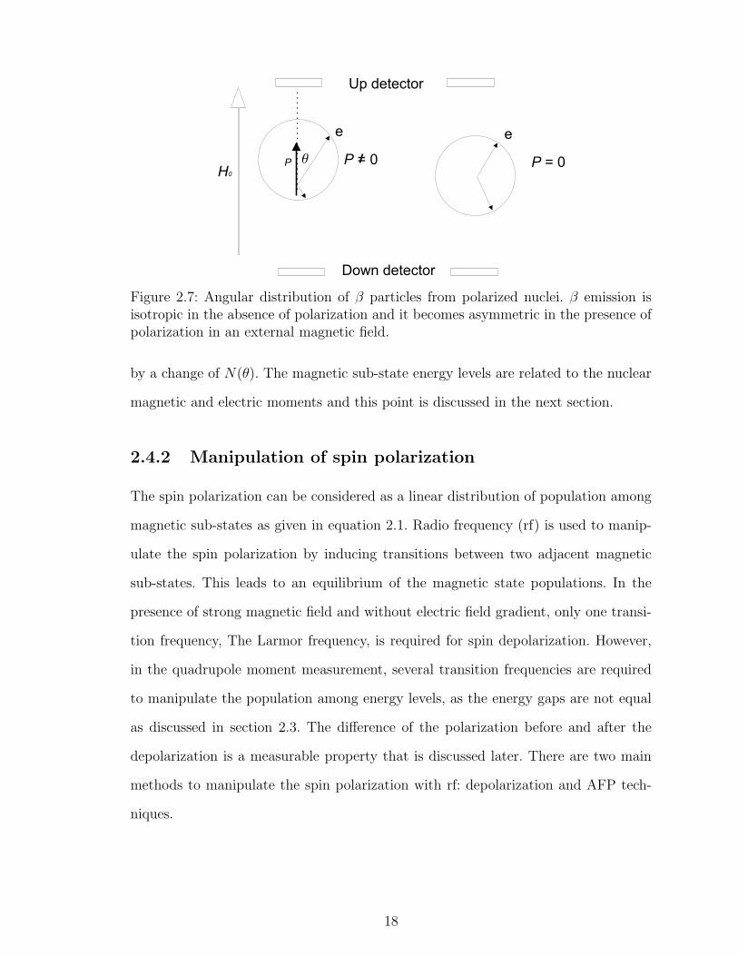
β decay is caused by the weak interaction which violates parity conservation [12].

Therefore, the angular distribution of β-particle emission is not symmetric relative to

the polarization direction as shown in figure 2.7, where β-rays are detected by placing

two sets of β-ray detectors at 00 (up) and 1800 (down). The angular distribution of

β emission is given by equation,

N(θ) ∼ 1 + AP cos θ, (2.10)

where, N(θ) is the number of β particles detected at an angle θ between the direction

of β-ray and polarization P and A is the asymmetry parameter. The magnetic sub-

state energy levels can be examined by inducing a polarization change that is detected

16

f

f

f

f

q

q

f

f

q

q

0

0

0

0

H0

a)

b)

c)

d)

z

y

Y

x

X

Z

z

z

z

y

y

y

Y

Y

YX

X

X

Z

Z

Z

x

x

x

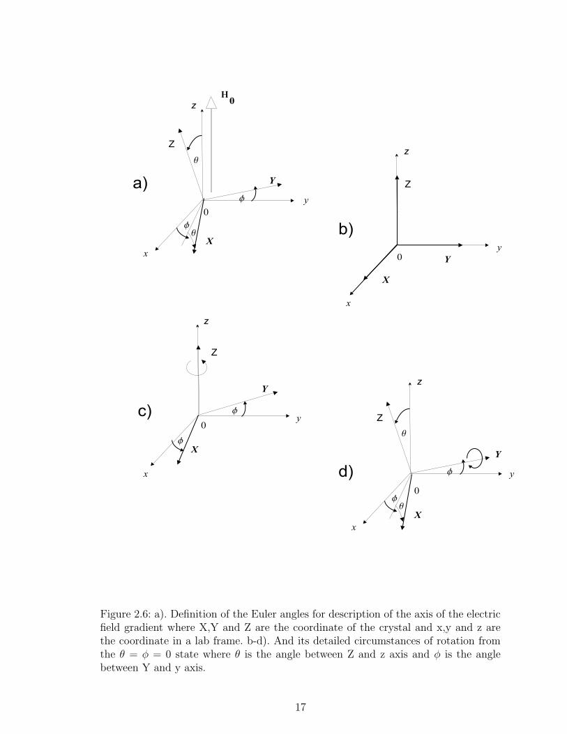
Figure 2.6: a). Definition of the Euler angles for description of the axis of the electricfield gradient where X,Y and Z are the coordinate of the crystal and x,y and z arethe coordinate in a lab frame. b-d). And its detailed circumstances of rotation fromthe θ = φ = 0 state where θ is the angle between Z and z axis and φ is the anglebetween Y and y axis.

17

q

ee

H0

P = 0P = 0

Up detector

Down detector

P

Figure 2.7: Angular distribution of β particles from polarized nuclei. β emission isisotropic in the absence of polarization and it becomes asymmetric in the presence ofpolarization in an external magnetic field.

by a change of N(θ). The magnetic sub-state energy levels are related to the nuclear

magnetic and electric moments and this point is discussed in the next section.

2.4.2 Manipulation of spin polarization

The spin polarization can be considered as a linear distribution of population among

magnetic sub-states as given in equation 2.1. Radio frequency (rf) is used to manip-

ulate the spin polarization by inducing transitions between two adjacent magnetic

sub-states. This leads to an equilibrium of the magnetic state populations. In the

presence of strong magnetic field and without electric field gradient, only one transi-

tion frequency, The Larmor frequency, is required for spin depolarization. However,

in the quadrupole moment measurement, several transition frequencies are required

to manipulate the population among energy levels, as the energy gaps are not equal

as discussed in section 2.3. The difference of the polarization before and after the

depolarization is a measurable property that is discussed later. There are two main

methods to manipulate the spin polarization with rf: depolarization and AFP tech-

niques.

18

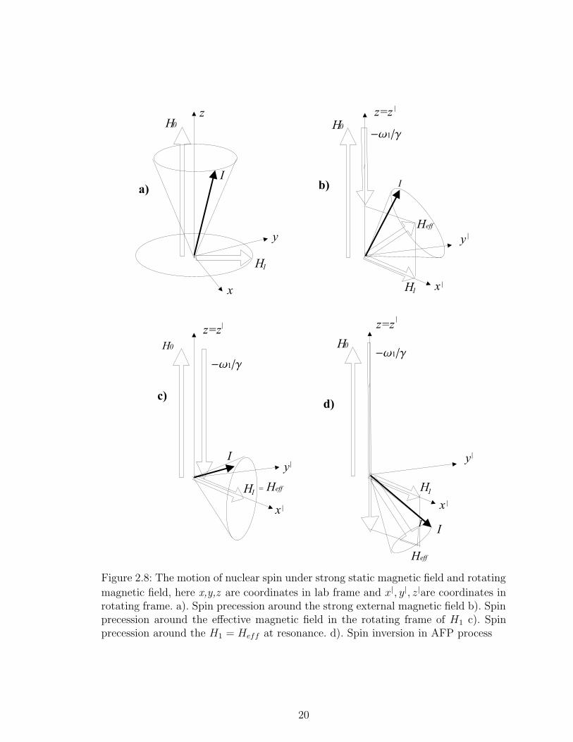
2.4.3 Depolarization technique

In the presence of a strong magnetic field H0, spin precesses around the field axis at

an angular frequency ω0. The equation of motion for spin precession is given as,

∂~I

∂t= γh~I × ~H0, (2.11)

where γ is the gyro-magnetic ratio. For NMR, an rf magnetic field H1, which rotates

at angular frequency ω1, is applied perpendicular to the H0 as shown in figure 2.8. In

the rotating frame of H1, nuclear spin feels effective magnetic field Heff and precesses

around Heff as shown in figure 2.8 b),

∂~I

∂t= γh~I × [ ~H0 +

~ω1

γ+ ~H1] ~Heff = [ ~H0 +

~ω1

γ+ ~H1]. (2.12)

At the resonance, ω1/γ is equal to H0 and H1 is equal to Heff . As a result, the spin

precesses around the Heff = H1 that is perpendicular to H0 as given in figure 2.8 c)

and as given in equation,

∂~I

∂t= γh~I × ~H1. (2.13)

Due to time averaging, the spin expectation value along the z-axis Iz becomes zero.

Therefore, spin polarization vanishes as it is defined as the expectation value of the

z-component Iz of the spin normalized by the total spin I as given in equation,

P =< Iz >

I. (2.14)

2.4.4 Adiabatic fast passage (AFP) technique

In this technique, the rf is swept once over the resonance frequency that results in an

inversion of the population between two adjacent magnetic sub-states. Two adiabatic

conditions have to be fulfilled to achieve efficient AFP process. Firstly, the rf magnetic

19

H0 H0

H0

z

y

H1

I

H1

H1

I

I

z=z

x|x

x|

y

|

y|

Heff

Heff=

-w /g1

-w /g1

b)

c)

a)

H0

H1

I

x|

y|

Heff

-w /g1

d)

I

|

z=z| z=z

|

Figure 2.8: The motion of nuclear spin under strong static magnetic field and rotating

magnetic field, here x,y,z are coordinates in lab frame and x|, y|, z|are coordinates inrotating frame. a). Spin precession around the strong external magnetic field b). Spinprecession around the effective magnetic field in the rotating frame of H1 c). Spinprecession around the H1 = Heff at resonance. d). Spin inversion in AFP process

20

field strength H1 and frequency sweeping speed should satisfy the first condition given

as,

(γNH1)2 À

∣

∣

∣

dω

dt

∣

∣

∣, (2.15)

where dω is the frequency modulation and dt is the frequency modulation time.

Secondly, H1 must be stronger than the local field HL at the nucleus given as,

γH1 À γHL. (2.16)

According to the relationship in 2.15, the sweeping speed should be less than the

angular velocity of spin precession around Heff so that the spin follows the change of

the effective magnetic field. In addition, according to the relationship in 2.16, the rf

magnetic field should be strong enough to prevent any coupling of the nuclear spins

with local fields. When there is a static magnetic field and perpendicular rf magnetic

field, the spin precesses around the effective field as explained in previous section.

Under the adiabatic conditions when the frequency is swept once, the direction of the

effective magnetic field is inverted. As a result, the bulk spin is also inverted as shown

in figure 2.8 d). Spin inversion makes the NMR signal two times larger than that in

depolarization technique as explain in the next section. However, higher rf magnetic

field strengths are required to satisfy the AFP condition compared with depolarization

technique. In the β-NQR technique, spin inversion needs several applied frequencies

in sequence. As an example for a I=3/2 nuclei, three transition frequencies rf1, rf2

and rf3 are required. Three frequencies have to be applied in a sequence of 1,2,3,1,2,1

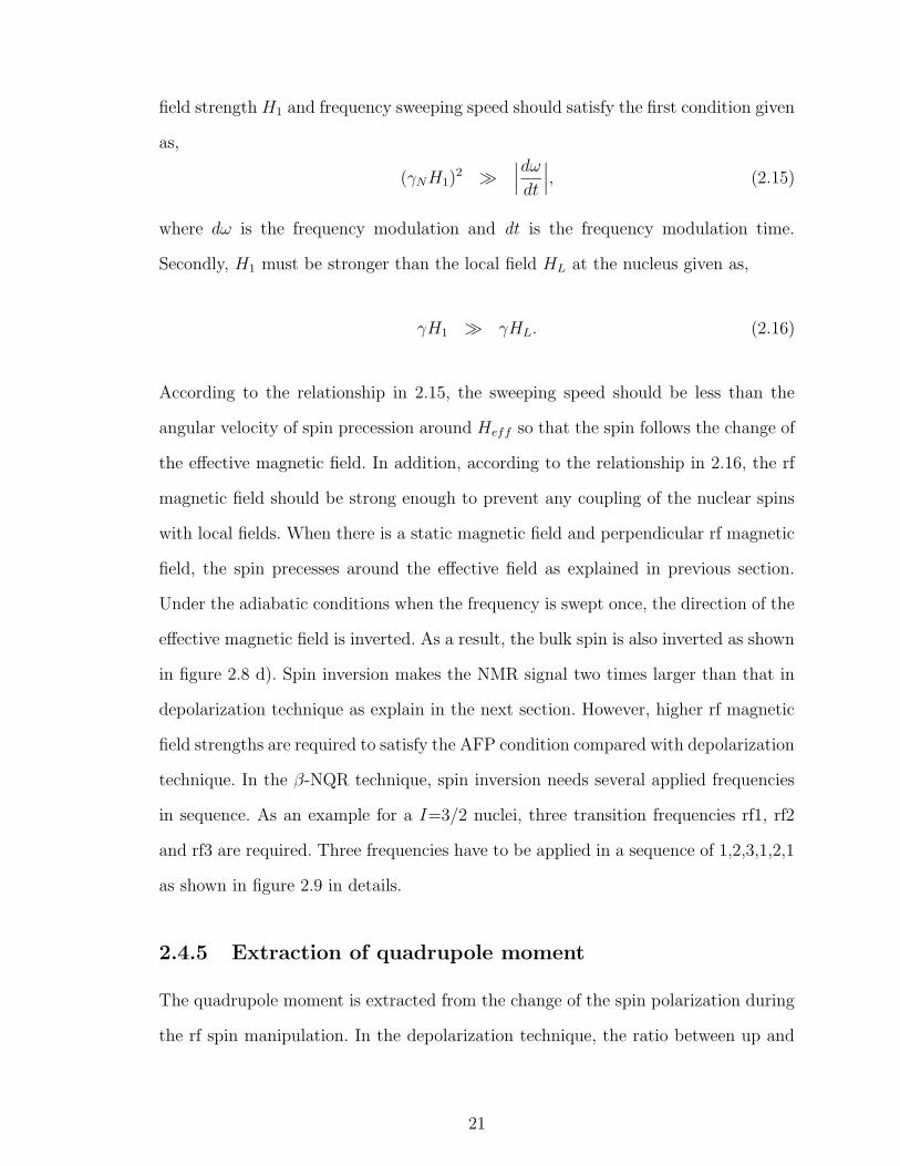
as shown in figure 2.9 in details.

2.4.5 Extraction of quadrupole moment

The quadrupole moment is extracted from the change of the spin polarization during

the rf spin manipulation. In the depolarization technique, the ratio between up and

21

Population

Transition frequency

rf1 rf2 rf3 rf1 rf2 rf1

-3/2

-1/2

1/2

3/2

Figure 2.9: In the case of I=3/2, spin inversion in AFP technique. Rf1 inverts the pop-ulation between magnetic state -3/2 and -1/2 and rf2 inverts the population between-1/2 and 1/2 states and so on. Total inversion of population occurs after applying thesequence of rf1, rf2, rf3, rf1, rf2 and rf1.

down counters is calculated for both rf field on (Ron) and off (Roff ),

Roff = gf1 + AP0

1 − AP0

Ron = gf1 + AP1

1 − AP1

. (2.17)

The difference ∆P = P0−P1 reflects the change in the magnetic sub-state population

distributed to the rf excitation, the geometrical factor, gf , is attributed to the imper-

fect symmetry of the experimental setup, for example, slight changes of efficiencies of

up and down counters. The geometrical factor is cancelled when the double ratio is

calculated as given in equation,

RD =Roff

Ron

≈ 1 + 2A(P0 − P1) = 1 + 2A∆P. (2.18)

The obtained signal RD is maximum when ∆P is maximum (∆P=P0 with P1=0). In

the AFP technique, the double ratio gives twice as large an asymmetry change than

in depolarization technique as shown in equations,

Roff = gf1 + AP0

1 − AP0

Ron = gf1 − AP0

1 + AP0

, (2.19)

22

RD =Roff

Ron

≈ 1 + 4AP0. (2.20)

One of the most important features in the quadrupole moment measurement is

that several transition frequencies are needed to manipulate the population among

energy levels, as energy gaps between adjacent m states are not equal to each other as

discussed in section 2.3. In depolarization technique, one resonance frequency equal-

izes population between two adjacent magnetic sub-states and reduces the spin po-

larization partially resulting in a small polarization change ∆P and hence small RD.

For I=3/2, the partial depolarization with one resonance frequency leads to only a

10% change of total asymmetry (A∆P ) and it needs hundred times more counting

time to reach the same statistics as in full depolarization, since the required time to

reach certain statistics is proportional to the figure of merit, 1/P 2Y, where Y is the

yield . These facts strongly indicate the importance of the total depolarization for a

reliable and an efficient measurement.

For I=3/2, the transition frequencies are calculated from equation 2.8 given in

sub-section 2.3, as a function of eqQ/h, and a set of three frequencies are applied

simultaneously. As discussed before, the split of highest and lowest transition fre-

quencies is proportional to νQ. If the RD is measured as a function of the electric

quadrupole-coupling constant νQ, at the true coupling constant there is resonance

as shown in figure 2.10. With the known electric field gradient of the host crystal,

the electric quadrupole moment can be extracted. For the extraction of quadrupole

moments are needed coupling constants of different isotopes measured in the same

crystal where one of the quadrupole moments is known,

Xknown

Xunknown

=Qknown

Qunknown

. (2.21)

Here, X represents the experimentally measured coupling constants.

23

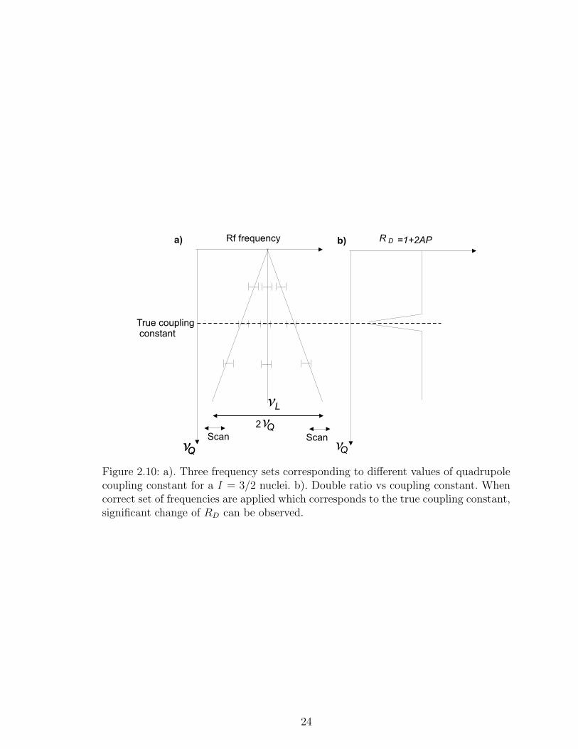
Rf frequency =1+2AP

True couplingconstant

R Da) b)

nQnQ

nQ2

nQ

nL

Scan Scan

Figure 2.10: a). Three frequency sets corresponding to different values of quadrupolecoupling constant for a I = 3/2 nuclei. b). Double ratio vs coupling constant. Whencorrect set of frequencies are applied which corresponds to the true coupling constant,significant change of RD can be observed.

24

Chapter 3

β-NQR Equipment Implementation

A β-NQR system is being implemented as an upgrade of the β-NMR system at the

NSCL with its β-NMR technique capabilities left intact. The β-NQR system can be

more efficient to perform β-NMR measurements as well. During the upgrade, sev-

eral important points were taken into consideration as summarized in the following

section. In a magnetic moment measurement with the β-NMR technique, only one

transition frequency is needed because the spacings are equal among the nuclear

magnetic sub-state energy levels under a strong external magnetic field. On the other

hand, in a quadrupole moment measurement with β-NQR technique, those spacings

become uneven as a result of the electric interactions introduced in the magnetically

interacting systems as explained in chapter 2. Therefore, the β-NQR system must

handle several different transition frequencies in sequences or almost simultaneously

in order to efficiently equalize or inverse the population of the magnetic sub-states.

Application of multiple-frequency NMR requires fast switching among these different

transition frequencies because the exotic nuclei of interest have very short life-times

(in millisecond range). Also, a high radio frequency (rf) magnetic field strength is

one of the important requirements for efficient measurements in both β-NMR and

β-NQR techniques, especially when the AFP technique is performed. A significant

current should flow through the rf coil to exert a high magnetic field (> 10G), which

25

RPV071

FG1 FG2 FG3

Mixer 50 W

Data U

RPV071

FG1 FG2 FG3 FG4

Six motor

drivers

250Wamplifier

50 W

Rf box

NMRchamber

Data U Vault

Gates

Driver

relayswitch

Spdaq

Relay switches

Variablecapacitors

VME bus

Rfcoil

Six

Logic signals

Rf signals

FG Function generators

LAN

LAN Local area network

Device server

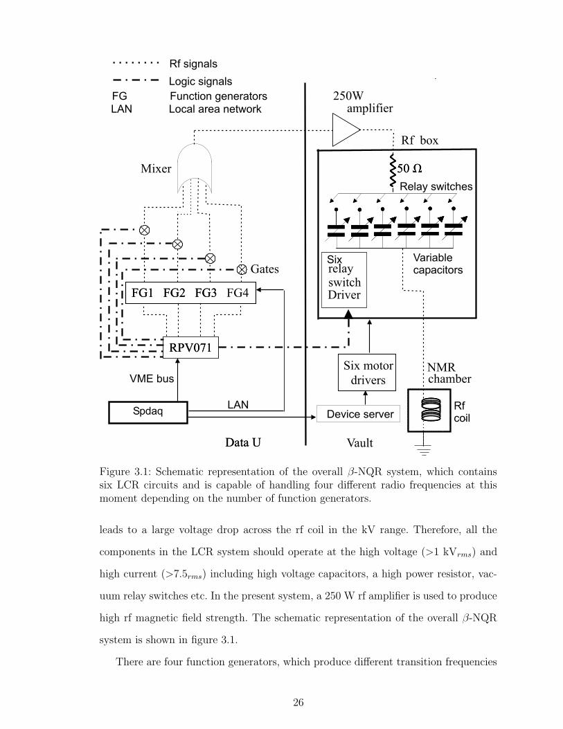
Figure 3.1: Schematic representation of the overall β-NQR system, which containssix LCR circuits and is capable of handling four different radio frequencies at thismoment depending on the number of function generators.

leads to a large voltage drop across the rf coil in the kV range. Therefore, all the

components in the LCR system should operate at the high voltage (>1 kVrms) and

high current (>7.5rms) including high voltage capacitors, a high power resistor, vac-

uum relay switches etc. In the present system, a 250 W rf amplifier is used to produce

high rf magnetic field strength. The schematic representation of the overall β-NQR

system is shown in figure 3.1.

There are four function generators, which produce different transition frequencies

26

relevant to specific electric coupling constant. A pulse pattern generator, RPV071,

triggers the function generators in sequence. Each rf signal is gated using the same

signal that triggers the function generator. After gating, the rf signal goes to a 250 W

rf amplifier and then to a LCR resonance circuit. A 50 Ω resistor or a transformer fulfill

the impedance matching between the amplifier and the rf coil. A 50 Ω resistor, six

variable capacitors and an rf coil make up virtually six independent LCR circuits. The

variable capacitors are controlled to tune the circuit to a specific frequency by stepper

motors, which are remotely controlled by stepper motor drivers. Relay switches are

used to select one of the LCR circuit out of six, depending on the transition frequency.

These relay switches are remotely controlled by a switch driver system to which TTL

control signals are sent by the RPV071 pulse pattern generators. An rf box contains

the impedance matching transformer, a 50 Ω resistor, six variable capacitors, six relay

switches, six relay switch drivers and a DC power supply for the switch drivers as

shown in figure 3.2. The rf coil, which produces rf magnetic field for NMR, is placed

in the vacuum chamber in the middle of the NMR magnet. The rf coil and the rf box

are connected by a coaxial 50 Ω cable. Each component will be explained in detail in

the following sections.

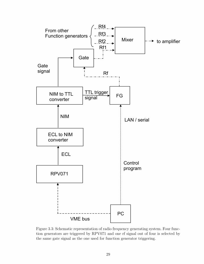
3.1 Radio frequency generation

Four different radio frequencies can be handled in the present system using four

function generators manufactured by Agilent Technologies. Some technical details of

the function generators are given in the table 3.1. The function generators can be

triggered internally or externally using TTL logic signal to start a linear frequency

sweep. The rf signals are gated by a module (X2M-01-411B / Pulser Corporation)

using trigger signals from RPV071. The rf signals from different function generators

are gathered to one path by a logic OR gate (433A / ORTEC) and sent to a 250 W

amplifier. The overall representation of the radio frequency generation and related

27

Stepper motors

Variablecapacitors

50 W resistor

Rf input

Rf output

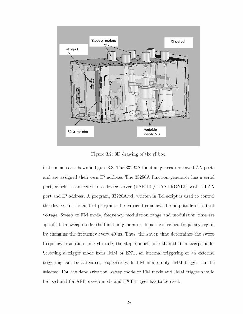
Figure 3.2: 3D drawing of the rf box.

instruments are shown in figure 3.3. The 33220A function generators have LAN ports

and are assigned their own IP address. The 33250A function generator has a serial

port, which is connected to a device server (USB 10 / LANTRONIX) with a LAN

port and IP address. A program, 33220A.tcl, written in Tcl script is used to control

the device. In the control program, the carrier frequency, the amplitude of output

voltage, Sweep or FM mode, frequency modulation range and modulation time are

specified. In sweep mode, the function generator steps the specified frequency region

by changing the frequency every 40 ns. Thus, the sweep time determines the sweep

frequency resolution. In FM mode, the step is much finer than that in sweep mode.

Selecting a trigger mode from IMM or EXT, an internal triggering or an external

triggering can be activated, respectively. In FM mode, only IMM trigger can be

selected. For the depolarization, sweep mode or FM mode and IMM trigger should

be used and for AFP, sweep mode and EXT trigger has to be used.

28

PC

RPV071

ECL to NIMconverter

NIM to TTLconverter

FG

Gate

Mixer to amplifier

ECL

NIM

Gatesignal

TTL triggersignal

Rf

Controlprogram

LAN / serial

VME bus

Rf1

Rf2

Rf3

Rf4From otherFunction generators

Figure 3.3: Schematic representation of radio frequency generating system. Four func-tion generators are triggered by RPV071 and one rf signal out of four is selected bythe same gate signal as the one used for function generator triggering.

29

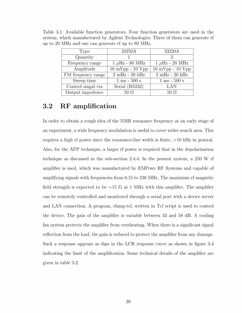
Table 3.1: Available function generators. Four function generators are used in thesystem, which manufactured by Agilent Technologies. Three of them can generate rfup to 20 MHz and one can generate rf up to 80 MHz.

Type 33250A 33220AQuantity 1 3

Frequency range 1 µHz - 80 MHz 1 µHz - 20 MHzAmplitude 10 mVpp - 10 Vpp 10 mVpp - 10 Vpp

FM frequency range 2 mHz - 20 kHz 2 mHz - 20 kHzSweep time 1 ms - 500 s 1 ms - 500 s

Control singal via Serial (RS232) LANOutput impedence 50 Ω 50 Ω

3.2 RF amplification

In order to obtain a rough idea of the NMR resonance frequency at an early stage of

an experiment, a wide frequency modulation is useful to cover wider search area. This

requires a high rf power since the resonance-line width is finite, <10 kHz in general.

Also, for the AFP technique, a larger rf power is required that in the depolarization

technique as discussed in the sub-section 2.4.4. In the present system, a 250 W rf

amplifier is used, which was manufactured by EMPowr RF Systems and capable of

amplifying signals with frequencies from 0.15 to 230 MHz. The maximum rf magnetic

field strength is expected to be ∼15 G at 1 MHz with this amplifier. The amplifier

can be remotely controlled and monitored through a serial port with a device server

and LAN connection. A program, rfamp.tcl, written in Tcl script is used to control

the device. The gain of the amplifier is variable between 33 and 58 dB. A cooling

fan system protects the amplifier from overheating. When there is a significant signal

reflection from the load, the gain is reduced to protect the amplifier from any damage.

Such a response appears as dips in the LCR response curve as shown in figure 3.4

indicating the limit of the amplification. Some technical details of the amplifier are

given in table 3.2.

30

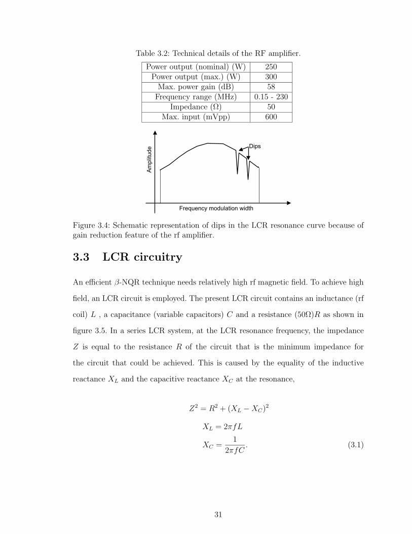
Table 3.2: Technical details of the RF amplifier.

Power output (nominal) (W) 250Power output (max.) (W) 300

Max. power gain (dB) 58Frequency range (MHz) 0.15 - 230

Impedance (Ω) 50Max. input (mVpp) 600

Am

plit

ude

Frequency modulation width

Dips

Figure 3.4: Schematic representation of dips in the LCR resonance curve because ofgain reduction feature of the rf amplifier.

3.3 LCR circuitry

An efficient β-NQR technique needs relatively high rf magnetic field. To achieve high

field, an LCR circuit is employed. The present LCR circuit contains an inductance (rf

coil) L , a capacitance (variable capacitors) C and a resistance (50Ω)R as shown in

figure 3.5. In a series LCR system, at the LCR resonance frequency, the impedance

Z is equal to the resistance R of the circuit that is the minimum impedance for

the circuit that could be achieved. This is caused by the equality of the inductive

reactance XL and the capacitive reactance XC at the resonance,

Z2 = R2 + (XL − XC)2

XL = 2πfL

XC =1

2πfC. (3.1)

31

Table 3.3: Technical details of the vacuum variable capacitors.

Model number CVDD-1000-15S C/UCSXF 1500 CMV1-4000-0005Type ceramic glass ceramic

Number of capacitors 2 2 2Capacity range (pF) 25 - 1000 20 - 1500 25 - 4000

Max. voltage peak (kV) 9.0 4.5 5.0Turn number 24 30 12

L

CA

B

Fromamplifier

R

Ferrite core

Figure 3.5: Schematic representation of the LCR circuit, where A represents 50 Ωimpedance matching resistor and B is the impedance matching transformer. Path Aor B will be selected depending on the experimental conditions.

When XL is equal to XC , the impedance of the system becomes R and the frequency

that gives this condition is called the resonance frequency given by,

fR =1

2π√

LC. (3.2)

By changing L and/or C the resonance frequency varies. The C is varied using variable

capacitors to tune the system for a specific frequency. There are six vacuum variable

capacitors, manufactured by Jennings Technology, and their technical details are pre-

sented in table 3.3. The capacitors are remotely tuned by stepper motors, which are

explained in section 3.5. Impedance of the LCR circuit should be matched to the out-

put impedance of the amplifier, which is 50 Ω. The impedance matching minimizes a

reflection of the rf signal back to the amplifier from the LCR circuit that distorts the

rf signal. There are two options in the system to match the impedance. One is to use

32

a 50 Ω, 250 W resistor and the other is to use an impedance matching transformer.

The transformer has two coils around a ferrite core: the primary coil is connected to

the rf amplifier and the secondary coil is connected to rf coil. Impedance matching of

the transformer is achieved using the relation,

RP

N2P

=RS

N2S

, (3.3)

where the RP and RS are the resistances and NP and NS are the turn numbers of

primary and secondary coils, respectively. Nominal resistance of the secondary coil is

∼1 Ω, the turn number is ∼ Np/Ns = 1/7.

A Quality factor Q, which is given by,

Q =2πfL

R=

f

∆f, (3.4)

defines the resonance response of the LCR circuit. The Q is lower for the resistor

system because the R is equal to 50 Ω compared with R ∼ 1 Ω of transformer system.

As a result, the 50 Ω resistor gives a low magnetic field strength but a broad power

output distribution over a wider frequency range; most useful in the depolarization

technique. On the other hand, the Q is higher for the transformer system in a narrower

frequency range that is useful in the AFP technique.

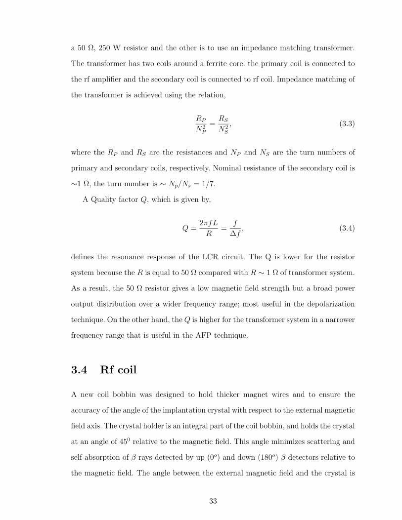
3.4 Rf coil

A new coil bobbin was designed to hold thicker magnet wires and to ensure the

accuracy of the angle of the implantation crystal with respect to the external magnetic

field axis. The crystal holder is an integral part of the coil bobbin, and holds the crystal

at an angle of 450 relative to the magnetic field. This angle minimizes scattering and

self-absorption of β rays detected by up (0o) and down (180o) β detectors relative to

the magnetic field. The angle between the external magnetic field and the crystal is

33

Catcher holder

Groove for the coil

Beam

Crystal holderRf arm H0

Bobbin

a).

b).

1’’

b detector

Figure 3.6: a). 3D drawing of the rf coil bobbin. b). Schematic presentation of theorientation of the coil bobbin. Catcher holder is an integral part of the bobbin andholds the crystal with an angle of 45o with respect to the Ho.

0o. There is minimum angular dependence of rf transition frequency as a function of

this angle. A schematic representation of the coil bobbin is given in figure 3.6. Several

rf coils were made with the same bobbin shape and different turn numbers. Each

rf coil has two equal windings in a Helmholtz-like geometry to achieve a uniform rf

magnetic field in the location of the host crystal. All rf coils were wound using gauge

24, Belden magnet wire (8078). A thicker wire was required to decrease the heat

generation as the high voltage drop across the coil. The inductances of the coils were

34

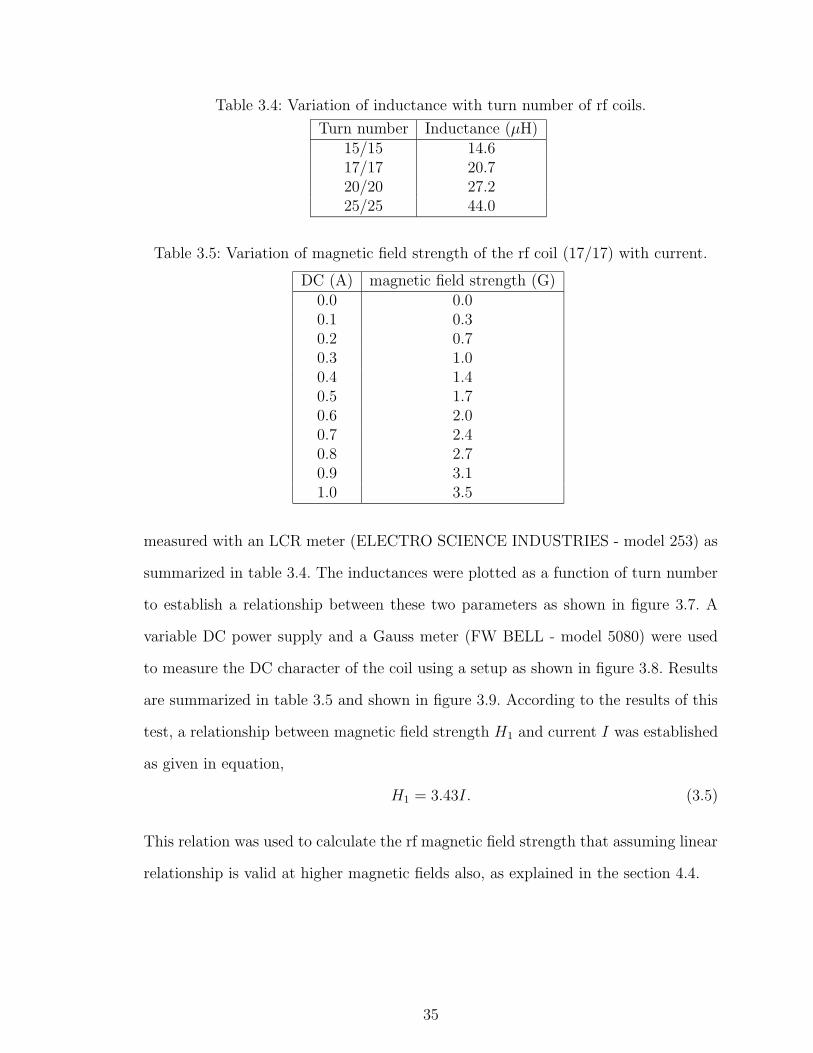
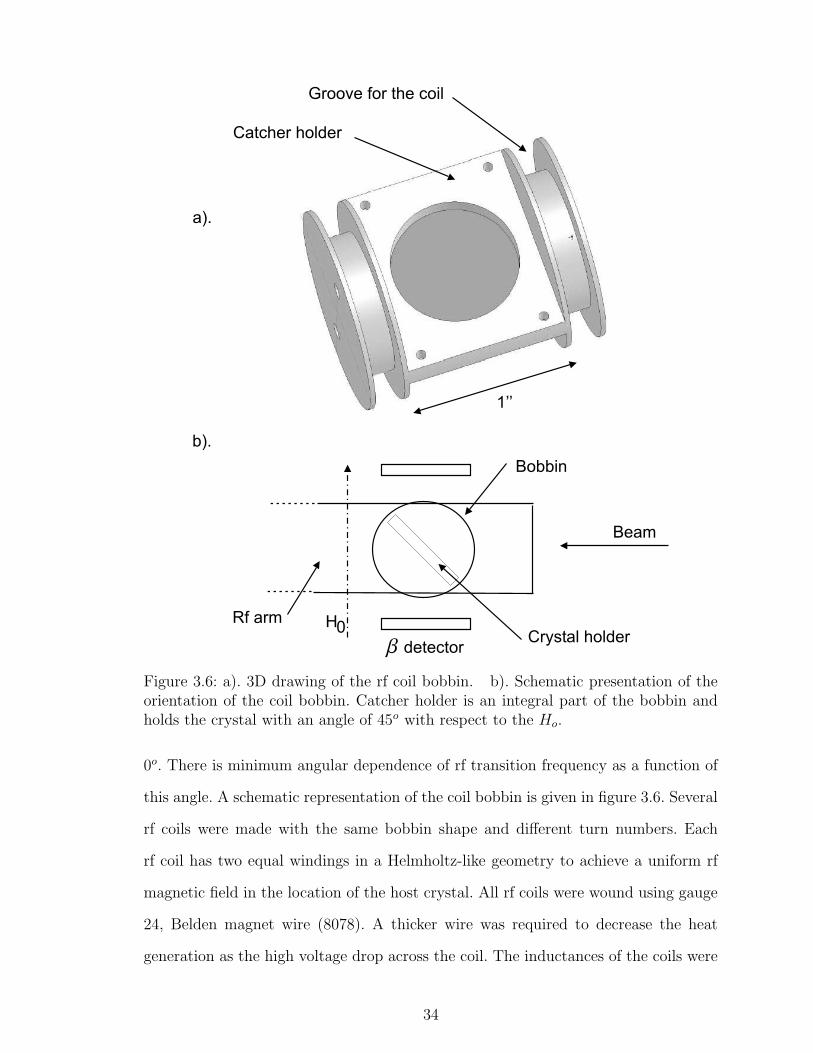
Table 3.4: Variation of inductance with turn number of rf coils.

Turn number Inductance (µH)15/15 14.617/17 20.720/20 27.225/25 44.0

Table 3.5: Variation of magnetic field strength of the rf coil (17/17) with current.

DC (A) magnetic field strength (G)0.0 0.00.1 0.30.2 0.70.3 1.00.4 1.40.5 1.70.6 2.00.7 2.40.8 2.70.9 3.11.0 3.5

measured with an LCR meter (ELECTRO SCIENCE INDUSTRIES - model 253) as

summarized in table 3.4. The inductances were plotted as a function of turn number

to establish a relationship between these two parameters as shown in figure 3.7. A

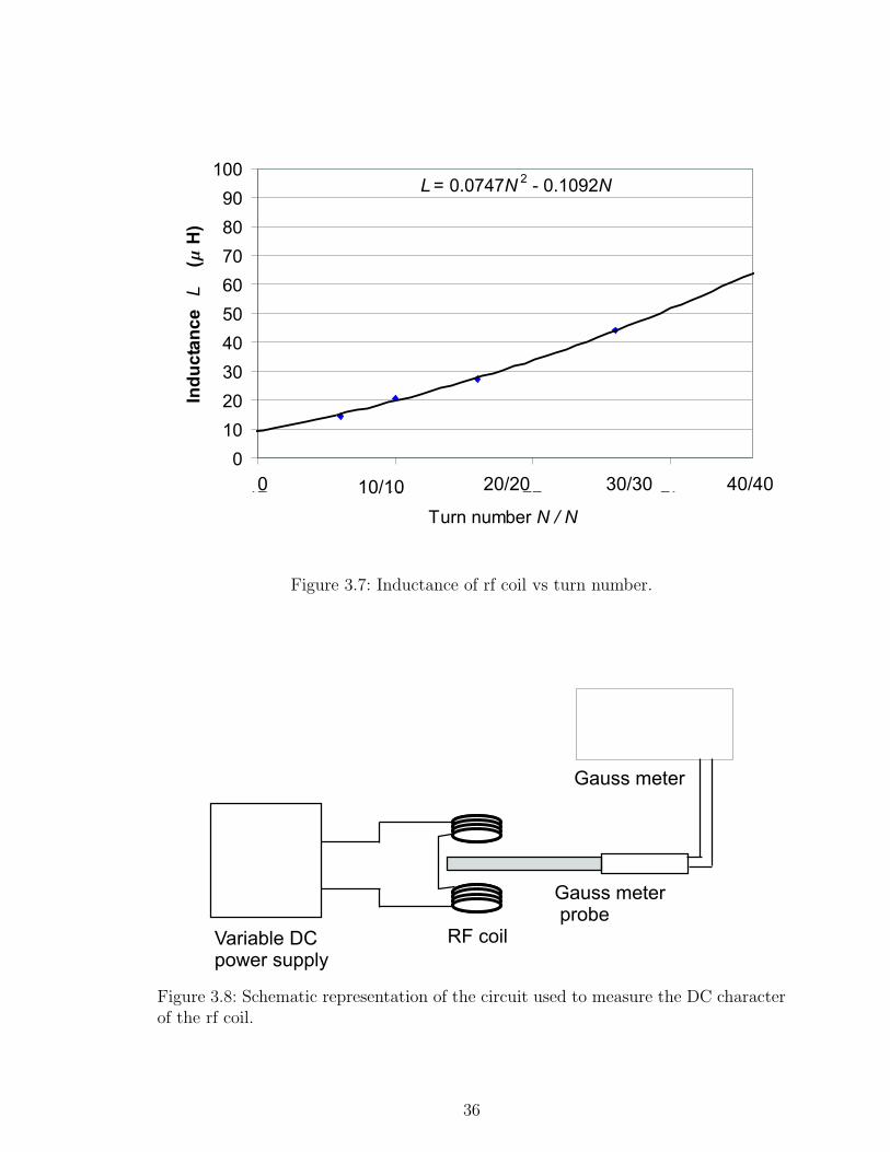
variable DC power supply and a Gauss meter (FW BELL - model 5080) were used

to measure the DC character of the coil using a setup as shown in figure 3.8. Results

are summarized in table 3.5 and shown in figure 3.9. According to the results of this

test, a relationship between magnetic field strength H1 and current I was established

as given in equation,

H1 = 3.43I. (3.5)

This relation was used to calculate the rf magnetic field strength that assuming linear

relationship is valid at higher magnetic fields also, as explained in the section 4.4.

35

L = 0.0747N2

- 0.1092N

0

10

20

30

40

50

60

70

80

90

100

12 17 22 27

Turn number N / N

Ind

ucta

nce

L(m

H)

10/10 20/20 30/30 40/400

Figure 3.7: Inductance of rf coil vs turn number.

Variable DCpower supply

RF coil

Gauss meterprobe

Gauss meter

Figure 3.8: Schematic representation of the circuit used to measure the DC characterof the rf coil.

36

H 1 = 3.4312I

0

0.5

1

1.5

2

2.5

3

3.5

4

0 0.2 0.4 0.6 0.8 1 1.2

Current I (A)

Magnetic

field

H1

(G)

Figure 3.9: Magnetic field strength of the 17/17 coil as a function of direct current.

Table 3.6: Node address hardware configuration.

Node addressesJ3 1 2 3 4 5 6 7 8 9 10 11 12 13 14 15 161 X X X X X X X X2 X X X X X X X X3 X X X X X X X X4 X X X X X X X X

3.5 Stepper motor controlling system

In experiments to search a nuclear quadrupole resonance by scanning the rf, different

of rf signals have to be applied. For each signal, the capacitors require adjustment to

have correct impedance matching. The variable capacitors are remotely adjusted by

stepper motors, which are driven by motor controllers with serial port connected to a

device server and LAN. The program testR4.tcl is a Tcl script written to control the

stepper motors. The motor controllers are manufactured by Eggert Electronics, model

37

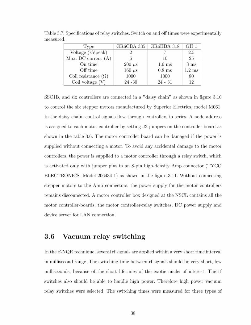
Table 3.7: Specifications of relay switches. Switch on and off times were experimentallymeasured.

Type GR6CBA 335 GR6HBA 318 GH 1Voltage (kVpeak) 2 7 2.5

Max. DC current (A) 6 10 25On time 200 µs 1.6 ms 3 msOff time 160 µs 0.8 ms 1.2 ms

Coil resistance (Ω) 1000 1000 80Coil voltage (V) 24 -30 24 - 31 12

SSC1B, and six controllers are connected in a ”daisy chain” as shown in figure 3.10

to control the six stepper motors manufactured by Superior Electrics, model M061.

In the daisy chain, control signals flow through controllers in series. A node address

is assigned to each motor controller by setting J3 jumpers on the controller board as

shown in the table 3.6. The motor controller board can be damaged if the power is

supplied without connecting a motor. To avoid any accidental damage to the motor

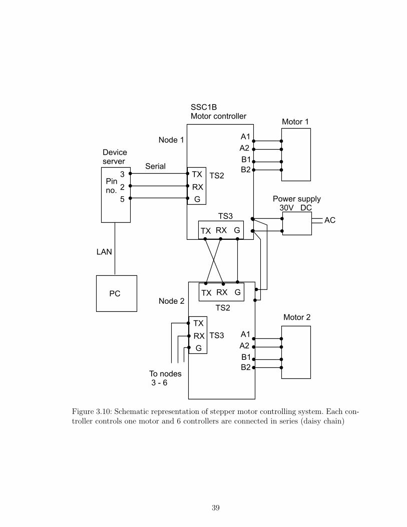
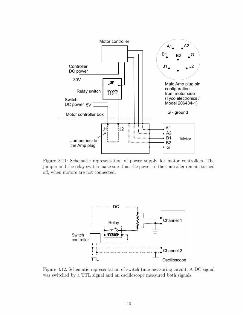
controllers, the power is supplied to a motor controller through a relay switch, which

is activated only with jumper pins in an 8-pin high-density Amp connector (TYCO

ELECTRONICS- Model 206434-1) as shown in the figure 3.11. Without connecting

stepper motors to the Amp connectors, the power supply for the motor controllers

remains disconnected. A motor controller box designed at the NSCL contains all the

motor controller-boards, the motor controller-relay switches, DC power supply and

device server for LAN connection.

3.6 Vacuum relay switching

In the β-NQR technique, several rf signals are applied within a very short time interval

in millisecond range. The switching time between rf signals should be very short, few

milliseconds, because of the short lifetimes of the exotic nuclei of interest. The rf

switches also should be able to handle high power. Therefore high power vacuum

relay switches were selected. The switching times were measured for three types of

38

PC

SSC1BMotor controller

Power supply30V DC

LAN

Serial

AC

Deviceserver

2

3

5

RX

TX

G

TS2

TX RX G

TS3

TX RX G

TS2

RX

TX

G

Node 1

Node 2

To nodes3 - 6

A1

A2

B1

B2

A1

A2

B1

B2

Motor 1

Motor 2

TS3

Pinno.

Figure 3.10: Schematic representation of stepper motor controlling system. Each con-troller controls one motor and 6 controllers are connected in series (daisy chain)

39

Motor controller

Jumper insidethe Amp plug

Relay switch

30V

5V

A1 A2

B1 B2 G

J1 J2

J1 J2

Male Amp plug pinconfigurationfrom motor side(Tyco electronics /Model 206434-1)

G - ground

A1

A2B1B2G

Motor

Motor controller box

ControllerDC power

SwitchDC power

Figure 3.11: Schematic representation of power supply for motor controllers. Thejumper and the relay switch make sure that the power to the controller remain turnedoff, when motors are not connected.

DC

TTL

Switchcontroller

Relay

Oscilloscope

Channel 1

Channel 2

Figure 3.12: Schematic representation of switch time measuring circuit. A DC signalwas switched by a TTL signal and an oscilloscope measured both signals.

40

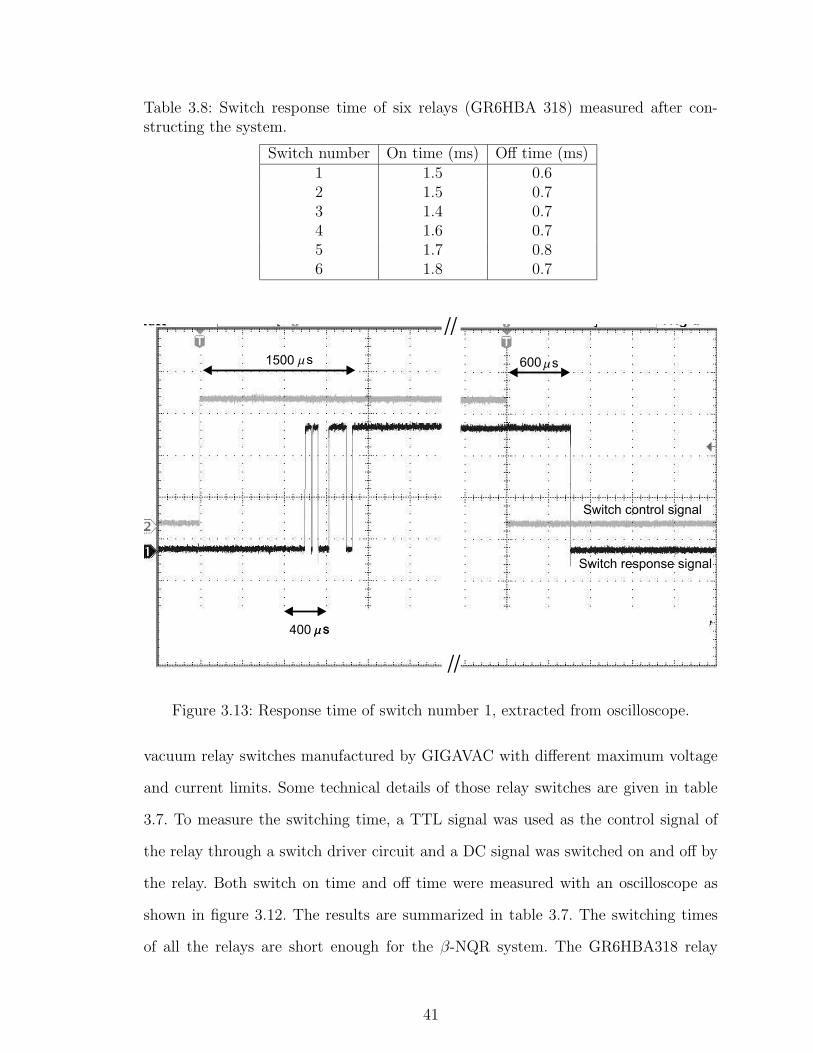
Table 3.8: Switch response time of six relays (GR6HBA 318) measured after con-structing the system.

Switch number On time (ms) Off time (ms)1 1.5 0.62 1.5 0.73 1.4 0.74 1.6 0.75 1.7 0.86 1.8 0.7

Switch control signal

Switch response signal

400 ms

//

//

1500 ms 600

ms

ms

Figure 3.13: Response time of switch number 1, extracted from oscilloscope.

vacuum relay switches manufactured by GIGAVAC with different maximum voltage

and current limits. Some technical details of those relay switches are given in table

3.7. To measure the switching time, a TTL signal was used as the control signal of

the relay through a switch driver circuit and a DC signal was switched on and off by

the relay. Both switch on time and off time were measured with an oscilloscope as

shown in figure 3.12. The results are summarized in table 3.7. The switching times

of all the relays are short enough for the β-NQR system. The GR6HBA318 relay

41

switch was selected for the system because of the high maximum voltage and current

and sufficient switching time, considering the decay lifetime of the 37K in the first

experiments that would be done to test the system as explained in the chapter 5.

However, depending on the experimental requirements, other types of relay switches

could be used. Six GR6HBA318 switches were purchased and installed in the rf box

and the switching times were checked for each relay. The results are summarized in

table 3.8 and a typical response is shown in figure 3.13. During the switch on time

period, a jitter was observed as the mechanical nature of the relays. A switch on time

of 2 ms would ensure that mechanical operation of relay close is complete.

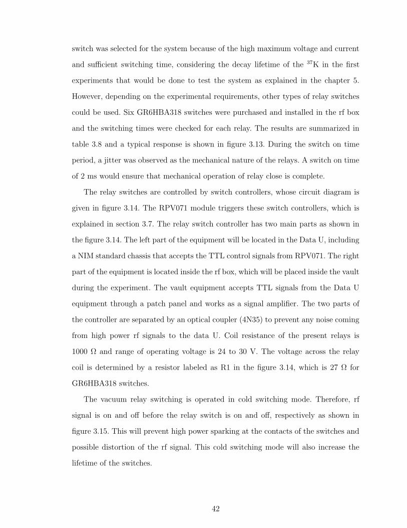
The relay switches are controlled by switch controllers, whose circuit diagram is

given in figure 3.14. The RPV071 module triggers these switch controllers, which is

explained in section 3.7. The relay switch controller has two main parts as shown in

the figure 3.14. The left part of the equipment will be located in the Data U, including

a NIM standard chassis that accepts the TTL control signals from RPV071. The right

part of the equipment is located inside the rf box, which will be placed inside the vault

during the experiment. The vault equipment accepts TTL signals from the Data U

equipment through a patch panel and works as a signal amplifier. The two parts of

the controller are separated by an optical coupler (4N35) to prevent any noise coming

from high power rf signals to the data U. Coil resistance of the present relays is

1000 Ω and range of operating voltage is 24 to 30 V. The voltage across the relay

coil is determined by a resistor labeled as R1 in the figure 3.14, which is 27 Ω for

GR6HBA318 switches.

The vacuum relay switching is operated in cold switching mode. Therefore, rf

signal is on and off before the relay switch is on and off, respectively as shown in

figure 3.15. This will prevent high power sparking at the contacts of the switches and

possible distortion of the rf signal. This cold switching mode will also increase the

lifetime of the switches.

42

12V

TTL 1K

1N22221N2222

1K

1K

4N35

2K8K

F

7812

50m

0.1m F

0.1mF

1K

2N22222.4K

3mF

2N2222

220mF

1N914A

1K

27W

30V

Data U Vault

Relay

R1

Figure 3.14: Circuit diagram of relay switch controllers. The two parts of the circuitare separated by an optical coupler (4N35) to minimize the possible noise coming tothe data U from the rf box.

Switch controlsignal

Rf gatesignal

2ms 1ms

Relay on time Relay off time

Figure 3.15: Relay switch control and rf gate signals. The rf gate signal is open withinthe limits of switch control signal to avoid any hot switching.

43

Clock NIM toTTL

RPV071

ECL to NIMNIM toTTL

FG Relay switchcontrollers

Dataacquisitionsystem

Cyclotron rf

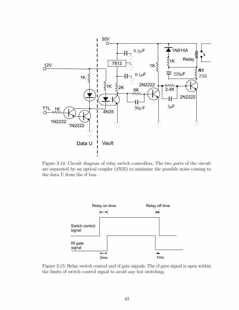
Figure 3.16: Schematic representation of triggering and timing system controlled bythe RPV071.

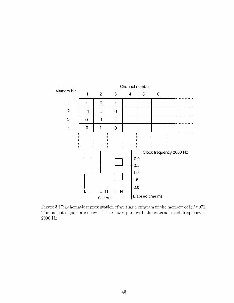
3.7 RPV071 module

RPV071 is a 32-channel pulse pattern generator manufactured by REPIC CORPO-

RATION according to the VME standards. The RPV071 controls all the triggering

and gating signals of experimental components and timing programs as shown in fig-

ure 3.16. A timing sequence is written to the memory of the RPV071 through the

VME bus. The memory of the RPV071 has 65K bins and each bin is divided into

32 channels. Writing 0 or 1 to each channel in the memory bins will result in low or

high output levels respectively, according to the clock signal given to the RPV071 as

shown in figure 3.17. Time resolution of the RPV071 depends on the clock signal that

can either be external or internal (50 MHz) source. As an example, if the frequency

of the clock signal is 2000 Hz, timing resolution is 0.5 ms (the bin position is incre-

mented every 0.5 ms). Since the total memory length is 65K long word, the maximum

time span would be about 30 s. For the proposed β-NQR experiments at the NSCL,

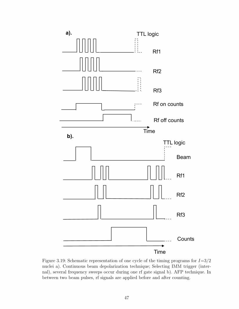
several timing programs will be used. Figure 3.18 shows a possible timing program

for the pulsed-beam depolarization method. Timing programs for continuous-beam

depolarization method and AFP method are shown schematically in figure 3.19 a) and

44

Channel numberMemory bin

1

2

3

4

1 0

1 2 3 4 5 6

0

0

0

1

1

1

1

1

0

0

Elapsed time ms

0.0

0.5

1.0

1.5

2.0

Out put

L H L H L H

Clock frequency 2000 Hz

Figure 3.17: Schematic representation of writing a program to the memory of RPV071.The output signals are shown in the lower part with the external clock frequency of2000 Hz.

45

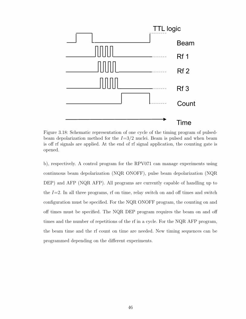
Beam

Rf 1

Rf 2

Rf 3

Count

TTL logic

Time

Figure 3.18: Schematic representation of one cycle of the timing program of pulsed-beam depolarization method for the I=3/2 nuclei. Beam is pulsed and when beamis off rf signals are applied. At the end of rf signal application, the counting gate isopened.

b), respectively. A control program for the RPV071 can manage experiments using

continuous beam depolarization (NQR ONOFF), pulse beam depolarization (NQR

DEP) and AFP (NQR AFP). All programs are currently capable of handling up to

the I=2. In all three programs, rf on time, relay switch on and off times and switch

configuration must be specified. For the NQR ONOFF program, the counting on and

off times must be specified. The NQR DEP program requires the beam on and off

times and the number of repetitions of the rf in a cycle. For the NQR AFP program,

the beam time and the rf count on time are needed. New timing sequences can be

programmed depending on the different experiments.

46

Rf1

Rf on counts

Rf off counts

Rf2

Rf3

a).

b).

Beam

Rf1

Rf2

Rf3

Counts

Time

Time

TTL logic

TTL logic

Figure 3.19: Schematic representation of one cycle of the timing programs for I=3/2nuclei a). Continuous beam depolarization technique; Selecting IMM trigger (inter-nal), several frequency sweeps occur during one rf gate signal b). AFP technique. Inbetween two beam pulses, rf signals are applied before and after counting.

47

Chapter 4

β-NQR system tests

Several tests were performed to evaluate individual components and the whole β-NQR

system.

4.1 Calibrating of stepper motor controllers for

variable capacitor operation

For the safety of the motor controlling system, upper and lower limits for the capac-

itors were set in the motor controlling program. A LCR meter was used to identify

the lowest and highest capacitance of each capacitor. Thereafter, the number of steps

taken by a stepper motor required to cover this range of capacitance was determined.

The turn number of a capacitor was calculated using the number of steps taken by a

stepper motor per revolution (200 steps/revolution). The results are summarized in

table 4.1.

48

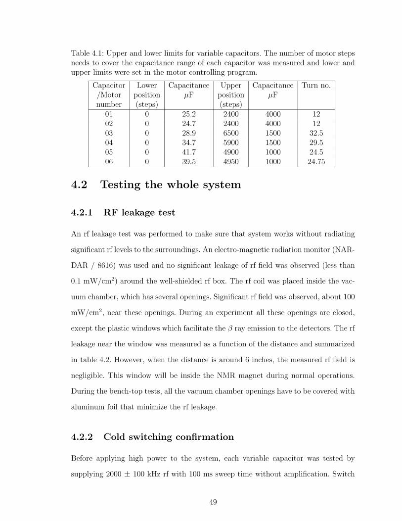
Table 4.1: Upper and lower limits for variable capacitors. The number of motor stepsneeds to cover the capacitance range of each capacitor was measured and lower andupper limits were set in the motor controlling program.

Capacitor Lower Capacitance Upper Capacitance Turn no./Motor position µF position µFnumber (steps) (steps)

01 0 25.2 2400 4000 1202 0 24.7 2400 4000 1203 0 28.9 6500 1500 32.504 0 34.7 5900 1500 29.505 0 41.7 4900 1000 24.506 0 39.5 4950 1000 24.75

4.2 Testing the whole system

4.2.1 RF leakage test

An rf leakage test was performed to make sure that system works without radiating

significant rf levels to the surroundings. An electro-magnetic radiation monitor (NAR-

DAR / 8616) was used and no significant leakage of rf field was observed (less than

0.1 mW/cm2) around the well-shielded rf box. The rf coil was placed inside the vac-

uum chamber, which has several openings. Significant rf field was observed, about 100

mW/cm2, near these openings. During an experiment all these openings are closed,

except the plastic windows which facilitate the β ray emission to the detectors. The rf

leakage near the window was measured as a function of the distance and summarized

in table 4.2. However, when the distance is around 6 inches, the measured rf field is

negligible. This window will be inside the NMR magnet during normal operations.

During the bench-top tests, all the vacuum chamber openings have to be covered with

aluminum foil that minimize the rf leakage.

4.2.2 Cold switching confirmation

Before applying high power to the system, each variable capacitor was tested by

supplying 2000 ± 100 kHz rf with 100 ms sweep time without amplification. Switch

49

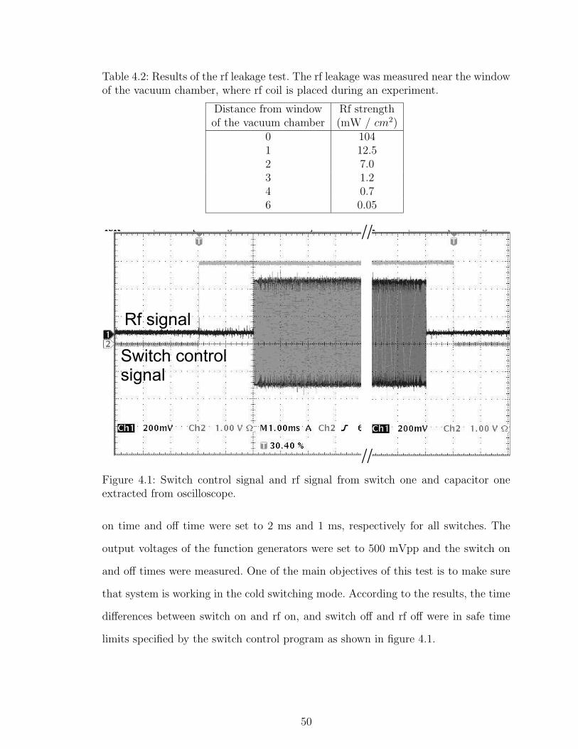
Table 4.2: Results of the rf leakage test. The rf leakage was measured near the windowof the vacuum chamber, where rf coil is placed during an experiment.

Distance from window Rf strengthof the vacuum chamber (mW / cm2)

0 1041 12.52 7.03 1.24 0.76 0.05

Rf signal

Switch controlsignal

//

//

Figure 4.1: Switch control signal and rf signal from switch one and capacitor oneextracted from oscilloscope.

on time and off time were set to 2 ms and 1 ms, respectively for all switches. The

output voltages of the function generators were set to 500 mVpp and the switch on

and off times were measured. One of the main objectives of this test is to make sure

that system is working in the cold switching mode. According to the results, the time

differences between switch on and rf on, and switch off and rf off were in safe time

limits specified by the switch control program as shown in figure 4.1.

50

700 kHz 1000 kHz 1300 kHz

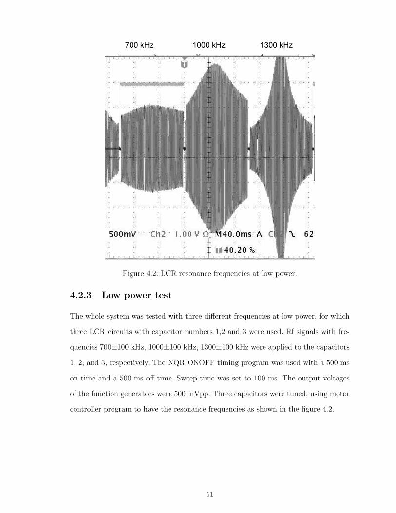
Figure 4.2: LCR resonance frequencies at low power.

4.2.3 Low power test

The whole system was tested with three different frequencies at low power, for which

three LCR circuits with capacitor numbers 1,2 and 3 were used. Rf signals with fre-

quencies 700±100 kHz, 1000±100 kHz, 1300±100 kHz were applied to the capacitors

1, 2, and 3, respectively. The NQR ONOFF timing program was used with a 500 ms

on time and a 500 ms off time. Sweep time was set to 100 ms. The output voltages

of the function generators were 500 mVpp. Three capacitors were tuned, using motor

controller program to have the resonance frequencies as shown in the figure 4.2.

51

Functiongenerator

Amplifier

Matchingtransformer

Variablecapacitor

Rf coil

Voltagedivider

Test point

Direct point

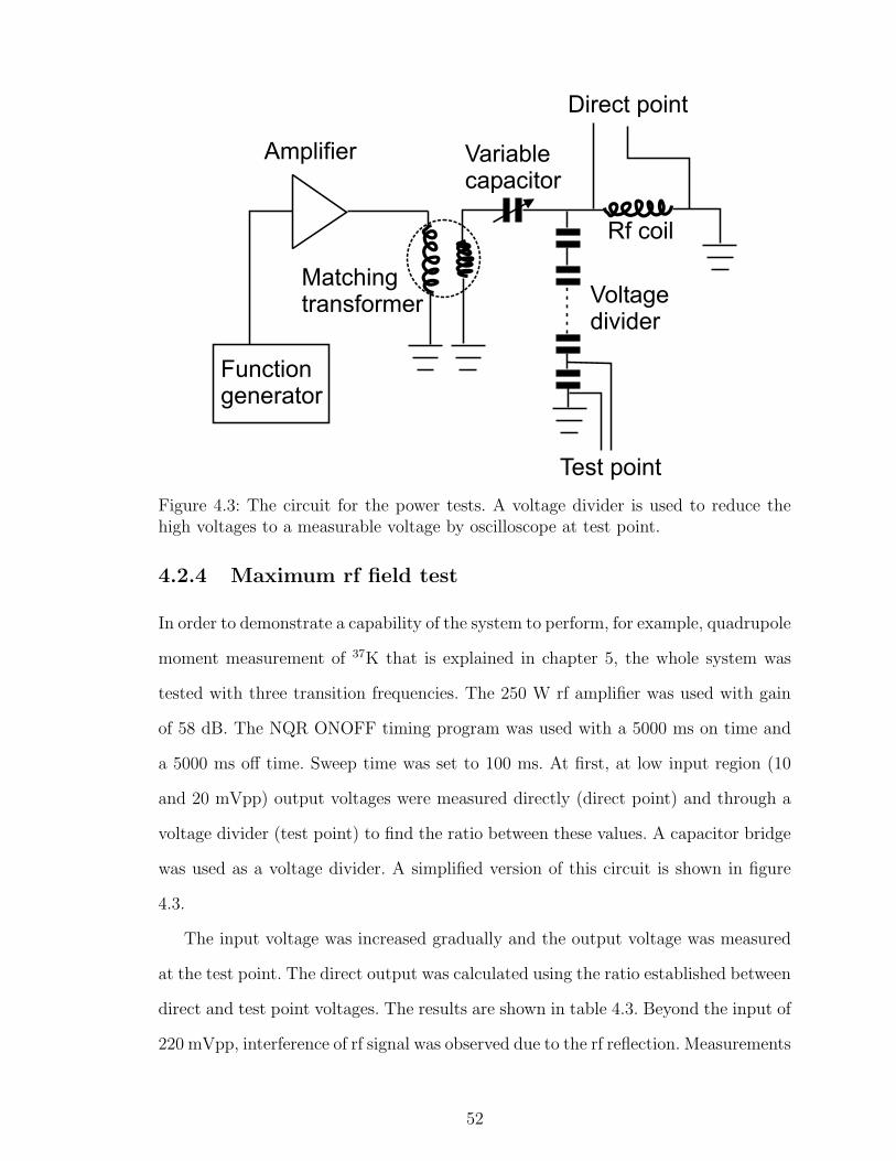
Figure 4.3: The circuit for the power tests. A voltage divider is used to reduce thehigh voltages to a measurable voltage by oscilloscope at test point.

4.2.4 Maximum rf field test

In order to demonstrate a capability of the system to perform, for example, quadrupole

moment measurement of 37K that is explained in chapter 5, the whole system was

tested with three transition frequencies. The 250 W rf amplifier was used with gain

of 58 dB. The NQR ONOFF timing program was used with a 5000 ms on time and

a 5000 ms off time. Sweep time was set to 100 ms. At first, at low input region (10

and 20 mVpp) output voltages were measured directly (direct point) and through a

voltage divider (test point) to find the ratio between these values. A capacitor bridge

was used as a voltage divider. A simplified version of this circuit is shown in figure

4.3.

The input voltage was increased gradually and the output voltage was measured

at the test point. The direct output was calculated using the ratio established between

direct and test point voltages. The results are shown in table 4.3. Beyond the input of

220 mVpp, interference of rf signal was observed due to the rf reflection. Measurements

52

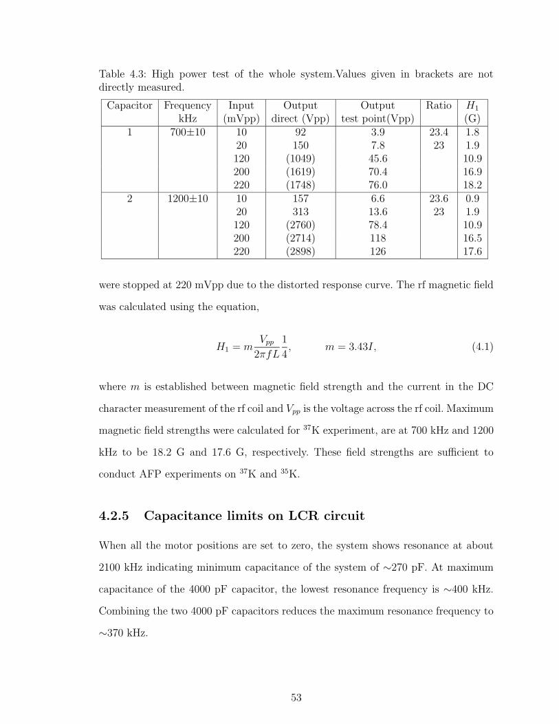
Table 4.3: High power test of the whole system.Values given in brackets are notdirectly measured.

Capacitor Frequency Input Output Output Ratio H1

kHz (mVpp) direct (Vpp) test point(Vpp) (G)1 700±10 10 92 3.9 23.4 1.8

20 150 7.8 23 1.9120 (1049) 45.6 10.9200 (1619) 70.4 16.9220 (1748) 76.0 18.2

2 1200±10 10 157 6.6 23.6 0.920 313 13.6 23 1.9120 (2760) 78.4 10.9200 (2714) 118 16.5220 (2898) 126 17.6

were stopped at 220 mVpp due to the distorted response curve. The rf magnetic field

was calculated using the equation,

H1 = mVpp

2πfL

1

4, m = 3.43I, (4.1)

where m is established between magnetic field strength and the current in the DC

character measurement of the rf coil and Vpp is the voltage across the rf coil. Maximum

magnetic field strengths were calculated for 37K experiment, are at 700 kHz and 1200

kHz to be 18.2 G and 17.6 G, respectively. These field strengths are sufficient to

conduct AFP experiments on 37K and 35K.

4.2.5 Capacitance limits on LCR circuit

When all the motor positions are set to zero, the system shows resonance at about

2100 kHz indicating minimum capacitance of the system of ∼270 pF. At maximum

capacitance of the 4000 pF capacitor, the lowest resonance frequency is ∼400 kHz.

Combining the two 4000 pF capacitors reduces the maximum resonance frequency to

∼370 kHz.

53

Chapter 5

β-NQR Application to 35,37K

The new β-NQR system is capable of measuring quadrupole moments of nuclei up

to I=2, according to the results of system tests explained in the last chapter. In this

chapter, the proposed experiments to measure quadrupole moments of the sd shell

nuclei 37K (Iπ=3/2+, t1/2=1.22 s) and 35K (Iπ=3/2+, t1/2=178 ms) are discussed.

5.1 Quadrupole moments of the nuclei in sd shell

A good agreement between experimental [2] and theoretical [13] (OXBASH) quadru-

pole moments for isospin T=1/2, sd shell nuclei, in general, is observed as shown in

figure 5.1. The trend of the quadrupole moments can be explained as follows. When

one single nucleon is in the 1d5/2 shell, the quadrupole moment takes a negative value.

The quadrupole moment changes sign as the 1d5/2 shell is filled, in agreement with

the single particle shell model. When the valence nucleons occupy the 2s1/2 orbit, the

quadrupole moment is zero, as the total angular momentum is equal to 1/2. When

the 1d3/2 shell has one nucleon, the quadrupole moment again is negative and changes

sign as the 1d3/2 shell is filled. The same type of systematic behavior of the quadru-

pole moment is expected for T=3/2 nuclei in the sd shell. However, as few (about

7 nuclei) measured quadrupole moments are available for T = 3/2 nuclei, especially

54

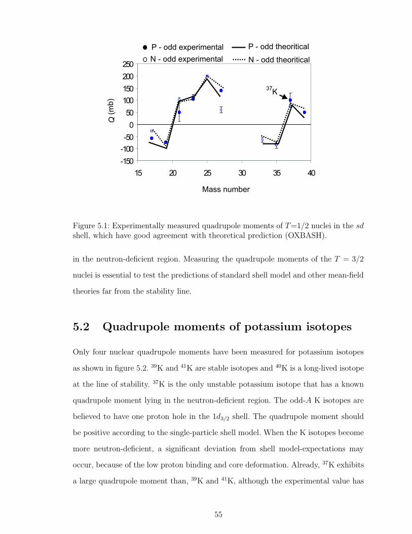
Fig 1. Quadrupole moments of T=1/2nuclei in the sd shell

-150

-100

-50

0

50

100

150

200

250

15 20 25 30 35 40

Massnumber

Qm

b

Mass number

Q(m

b)

K37

N - odd experimental

P - odd theoritical

N - odd theoritical

P - odd experimental

Figure 5.1: Experimentally measured quadrupole moments of T=1/2 nuclei in the sdshell, which have good agreement with theoretical prediction (OXBASH).

in the neutron-deficient region. Measuring the quadrupole moments of the T = 3/2

nuclei is essential to test the predictions of standard shell model and other mean-field

theories far from the stability line.

5.2 Quadrupole moments of potassium isotopes

Only four nuclear quadrupole moments have been measured for potassium isotopes

as shown in figure 5.2. 39K and 41K are stable isotopes and 40K is a long-lived isotope

at the line of stability. 37K is the only unstable potassium isotope that has a known

quadrupole moment lying in the neutron-deficient region. The odd-A K isotopes are

believed to have one proton hole in the 1d3/2 shell. The quadrupole moment should

be positive according to the single-particle shell model. When the K isotopes become

more neutron-deficient, a significant deviation from shell model-expectations may

occur, because of the low proton binding and core deformation. Already, 37K exhibits

a large quadrupole moment than, 39K and 41K, although the experimental value has

55

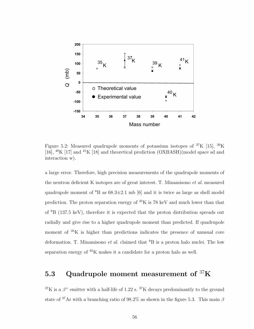
-150

-100

-50

0

50

100

150

200

34 35 36 37 38 39 40 41 42

Theoretical value

Experimental value

Q(m

b)

35K

37K 39

K

40K

41K

Mass number

Figure 5.2: Measured quadrupole moments of potassium isotopes of 37K [15], 39K[16], 40K [17] and 41K [18] and theoretical prediction (OXBASH)(model space sd andinteraction w).

a large error. Therefore, high precision measurements of the quadrupole moments of

the neutron deficient K isotopes are of great interest. T. Minamisono et al. measured

quadrupole moment of 8B as 68.3±2.1 mb [6] and it is twice as large as shell model

prediction. The proton separation energy of 35K is 78 keV and much lower than that

of 8B (137.5 keV), therefore it is expected that the proton distribution spreads out

radially and give rise to a higher quadrupole moment than predicted. If quadrupole

moment of 35K is higher than predictions indicates the presence of unusual core

deformation. T. Minamisono et al. claimed that 8B is a proton halo nuclei. The low

separation energy of 35K makes it a candidate for a proton halo as well.

5.3 Quadrupole moment measurement of 37K

37K is a β+ emitter with a half-life of 1.22 s. 37K decays predominantly to the ground

state of 37Ar with a branching ratio of 98.2% as shown in the figure 5.3. This main β

56

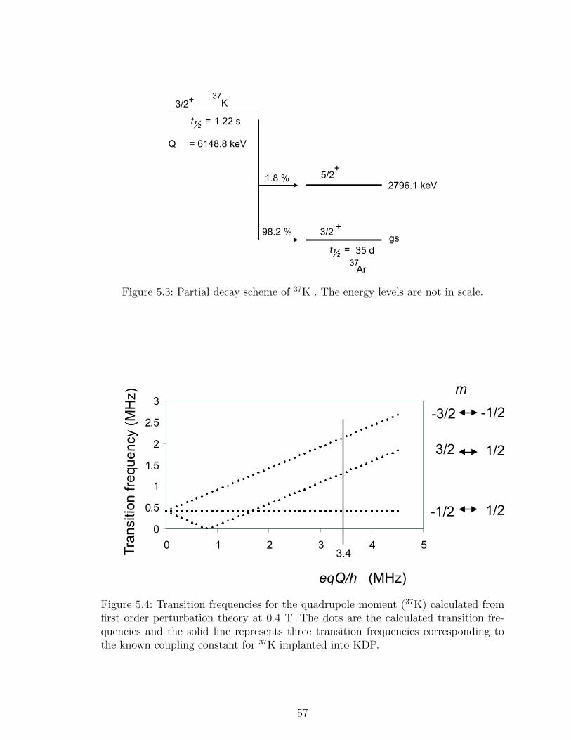
37K

Q = 6148.8 keV

3/2+

3/2+

5/2+

Ar37

t½ =

35 d

1.22 s

t½ =

98.2 %

1.8 %

gs

2796.1 keV

Figure 5.3: Partial decay scheme of 37K . The energy levels are not in scale.

0

0.5

1

1.5

2

2.5

3

0 1 2 3 4 5

X (MHz)

Tra

ns

fre

q.

MH

zT

ran

sitio

nfr

eq

ue

ncy (

MH

z)

eqQ/h (MHz)

3.4

-3/2 -1/2

3/2 1/2

-1/2 1/2

m

Figure 5.4: Transition frequencies for the quadrupole moment (37K) calculated fromfirst order perturbation theory at 0.4 T. The dots are the calculated transition fre-quencies and the solid line represents three transition frequencies corresponding tothe known coupling constant for 37K implanted into KDP.

57

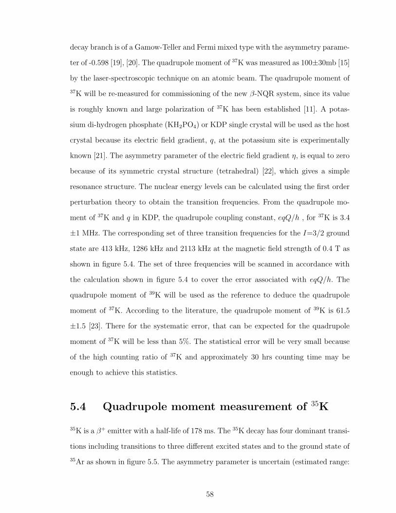
decay branch is of a Gamow-Teller and Fermi mixed type with the asymmetry parame-

ter of -0.598 [19], [20]. The quadrupole moment of 37K was measured as 100±30mb [15]

by the laser-spectroscopic technique on an atomic beam. The quadrupole moment of

37K will be re-measured for commissioning of the new β-NQR system, since its value

is roughly known and large polarization of 37K has been established [11]. A potas-

sium di-hydrogen phosphate (KH2PO4) or KDP single crystal will be used as the host

crystal because its electric field gradient, q, at the potassium site is experimentally

known [21]. The asymmetry parameter of the electric field gradient η, is equal to zero

because of its symmetric crystal structure (tetrahedral) [22], which gives a simple

resonance structure. The nuclear energy levels can be calculated using the first order

perturbation theory to obtain the transition frequencies. From the quadrupole mo-

ment of 37K and q in KDP, the quadrupole coupling constant, eqQ/h , for 37K is 3.4

±1 MHz. The corresponding set of three transition frequencies for the I=3/2 ground

state are 413 kHz, 1286 kHz and 2113 kHz at the magnetic field strength of 0.4 T as

shown in figure 5.4. The set of three frequencies will be scanned in accordance with

the calculation shown in figure 5.4 to cover the error associated with eqQ/h. The

quadrupole moment of 39K will be used as the reference to deduce the quadrupole

moment of 37K. According to the literature, the quadrupole moment of 39K is 61.5

±1.5 [23]. There for the systematic error, that can be expected for the quadrupole

moment of 37K will be less than 5%. The statistical error will be very small because

of the high counting ratio of 37K and approximately 30 hrs counting time may be

enough to achieve this statistics.

5.4 Quadrupole moment measurement of 35K

35K is a β+ emitter with a half-life of 178 ms. The 35K decay has four dominant transi-

tions including transitions to three different excited states and to the ground state of

35Ar as shown in figure 5.5. The asymmetry parameter is uncertain (estimated range:

58

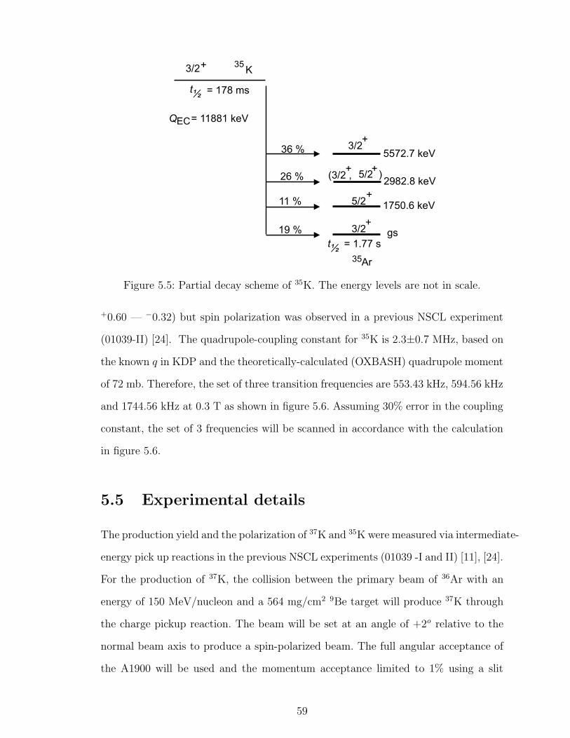
35K

t½

t½ = 178 ms

= 1.77 s

35Ar

Q = 11881 keV

+

3/2+

(3/2 ,+

3/2+

5/2 )

+5/2

36 %

26 %

19 %

11 %

3/2+

EC

5572.7 keV

2982.8 keV

1750.6 keV

gs

Figure 5.5: Partial decay scheme of 35K. The energy levels are not in scale.

+0.60 — −0.32) but spin polarization was observed in a previous NSCL experiment

(01039-II) [24]. The quadrupole-coupling constant for 35K is 2.3±0.7 MHz, based on

the known q in KDP and the theoretically-calculated (OXBASH) quadrupole moment

of 72 mb. Therefore, the set of three transition frequencies are 553.43 kHz, 594.56 kHz

and 1744.56 kHz at 0.3 T as shown in figure 5.6. Assuming 30% error in the coupling

constant, the set of 3 frequencies will be scanned in accordance with the calculation

in figure 5.6.

5.5 Experimental details

The production yield and the polarization of 37K and 35K were measured via intermediate-

energy pick up reactions in the previous NSCL experiments (01039 -I and II) [11], [24].

For the production of 37K, the collision between the primary beam of 36Ar with an

energy of 150 MeV/nucleon and a 564 mg/cm2 9Be target will produce 37K through

the charge pickup reaction. The beam will be set at an angle of +2o relative to the

normal beam axis to produce a spin-polarized beam. The full angular acceptance of

the A1900 will be used and the momentum acceptance limited to 1% using a slit

59

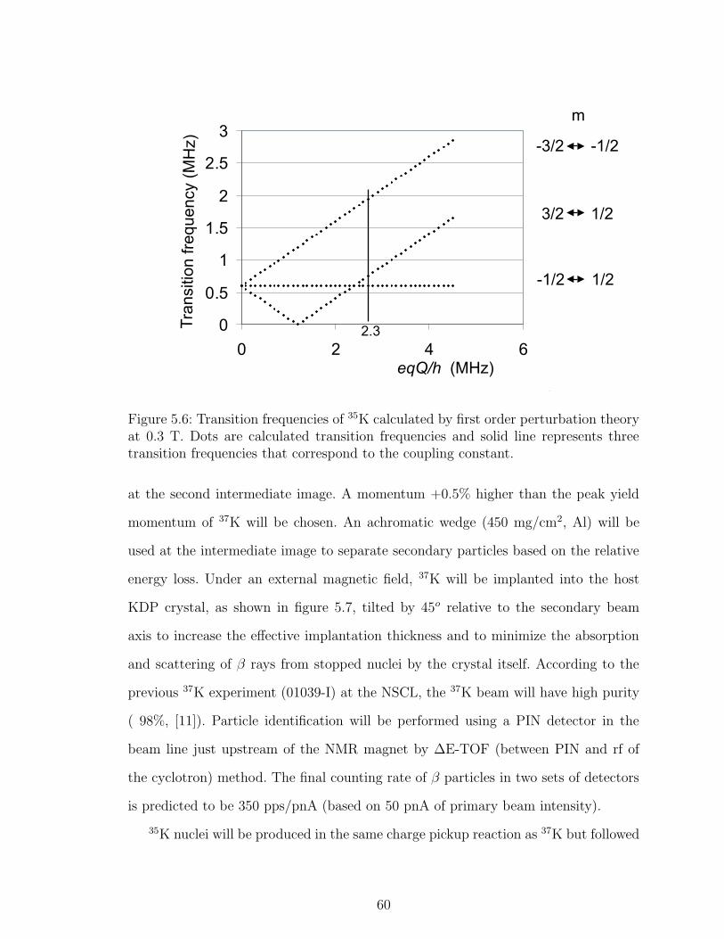
0

0.5

1

1.5

2

2.5

3

0 2 4 6

Tra

nsitio

nfr

eq

ue

ncy

(MH

z)

eqQ/h (MHz)

2.3

-3/2 -1/2

3/2 1/2

-1/2 1/2

m

Figure 5.6: Transition frequencies of 35K calculated by first order perturbation theoryat 0.3 T. Dots are calculated transition frequencies and solid line represents threetransition frequencies that correspond to the coupling constant.

at the second intermediate image. A momentum +0.5% higher than the peak yield

momentum of 37K will be chosen. An achromatic wedge (450 mg/cm2, Al) will be

used at the intermediate image to separate secondary particles based on the relative

energy loss. Under an external magnetic field, 37K will be implanted into the host

KDP crystal, as shown in figure 5.7, tilted by 45o relative to the secondary beam

axis to increase the effective implantation thickness and to minimize the absorption

and scattering of β rays from stopped nuclei by the crystal itself. According to the

previous 37K experiment (01039-I) at the NSCL, the 37K beam will have high purity

( 98%, [11]). Particle identification will be performed using a PIN detector in the

beam line just upstream of the NMR magnet by ∆E-TOF (between PIN and rf of

the cyclotron) method. The final counting rate of β particles in two sets of detectors

is predicted to be 350 pps/pnA (based on 50 pnA of primary beam intensity).

35K nuclei will be produced in the same charge pickup reaction as 37K but followed

60

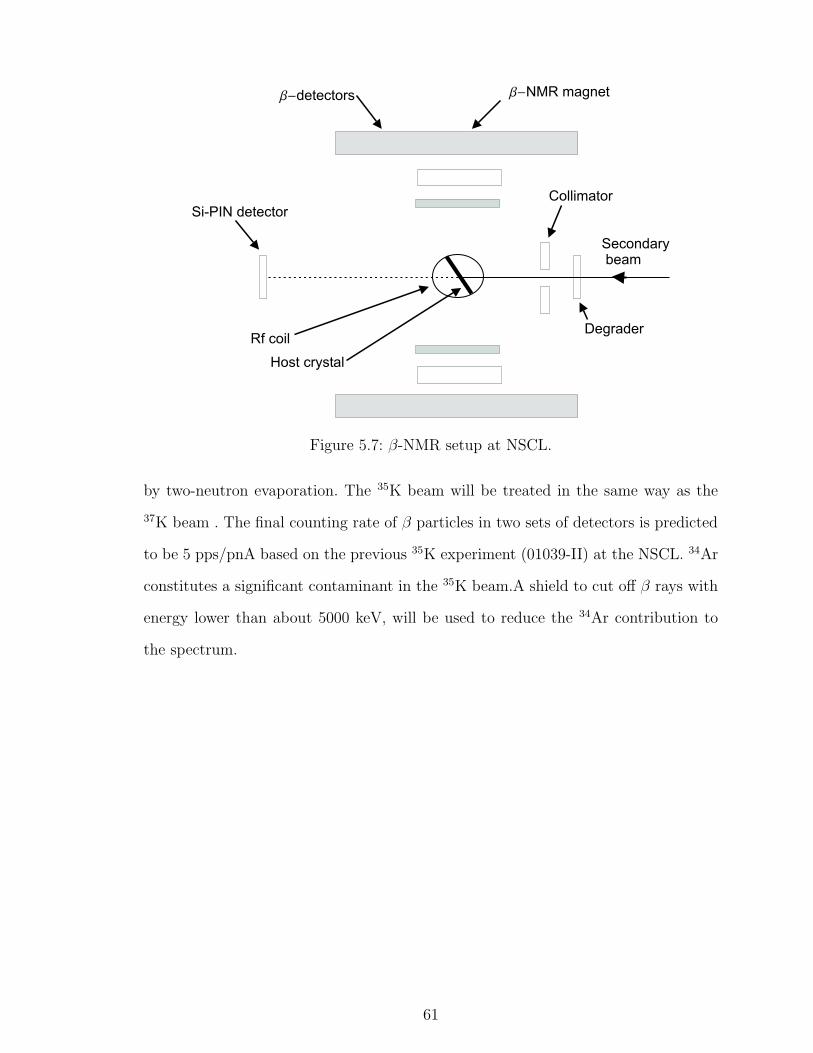
b-NMR magnetb-detectors

Si-PIN detectorCollimator

Degrader

Host crystal

Rf coil

Secondarybeam

Figure 5.7: β-NMR setup at NSCL.

by two-neutron evaporation. The 35K beam will be treated in the same way as the

37K beam . The final counting rate of β particles in two sets of detectors is predicted

to be 5 pps/pnA based on the previous 35K experiment (01039-II) at the NSCL. 34Ar

constitutes a significant contaminant in the 35K beam.A shield to cut off β rays with

energy lower than about 5000 keV, will be used to reduce the 34Ar contribution to

the spectrum.

61

Chapter 6

Summary

The Quadrupole moment is a direct measure of the deviation of charge distribution

of a nucleus from its spherical shape. Therefore, it is zero for spherical-shaped nuclei

and takes positive value and negative value for prolate-shaped and oblate-shaped

deformed nuclei, respectively.

The quadrupole moment is used as an important observable to investigate the

nuclear structure, as it changes sign over a shell indicating the presence of a proton

hole or an odd valence proton, respectively. The quadrupole moment can be used as

evidence for the presence of configuration mixing in the nucleus. Core deformation

is also a concept that can be investigated by quadruple moment measurements, es-

pecially in the heavy-mass nuclei. The measured large quadrupole moments of heavy

nuclei helped to establish the collective effects of valence nucleons on the core de-

formation. The quadrupole moment can be used to extract the charge radius of the

nucleus, which is important to understand the radial extent of a nucleus.

There are several techniques to measure the quadrupole moments including laser

spectroscopy, low temperature nuclear orientation, nuclear quadrupole resonance tech-

nique, and microwave spectroscopy. Each technique has its own advantages and dis-

advantages.

The β-NQR technique moreover, is probably the most effective method to mea-

62

sure nuclear electric quadrupole moments of exotic nuclei. The technique requires an

ensemble of spin-polarized β emitting nuclei. At the NSCL, nuclear spin polarization

is produced directly in intermediate-energy heavy-ion reactions. Both nucleon pickup

and removal reactions can be used to generate polarizations of order 1% or greater

for nuclei a few nucleons away from the projectile.

The β-NQR method requires a host material with a non-cubic lattice structure.

Polarized nuclei are implanted in a crystal with an electric field gradient placed in a

strong magnetic field. The strong magnetic field helps to preserve the spin polariza-

tion that can be depolarized due to the spin-lattice relaxation and spin-spin relaxation

processes. In addition, Zeeman splitting is induced by the magnetic field. The electric

interactions shift the evenly spaced energy levels because of the electric field gradient

of the host crystal. The spin manipulation is performed by applying rf magnetic field

perpendicular to the external magnetic field. Several different transition frequencies

are required for the depolarization because of the uneven energy gaps among mag-

netic sub-states. There are two spin manipulation techniques as depolarization and

AFP technique. In the depolarization technique, spin precesses around the effective

magnetic field that is a result of the external magnetic field and at the resonance, the

spin precess around the rf magnetic field and the spin polarization vanishes. In the

AFP technique, an rf is swept once over the resonance frequency that leads to the

spin inversion. The spin inversion makes the NMR effect two times larger, however,

it needs higher rf magnetic field than that in the depolarization method.

The β-NQR system described in this thesis was designed to meet the criteria listed

above. The system is an upgrade of the previous β-NMR system at the NSCL. It has

a multi rf capability, utilizing four function generators to produce four different tran-

sition frequencies. A 250 W rf amplifier is used to achieve the high magnetic field

for spin manipulation .A LCR circuit is used to match the output impedance of the

amplifier. A high voltage drop will exist in the LCR circuit and the individual com-

ponents of this circuit were chosen to be capable of handling high voltages. All the

63

variable vacuum capacitors can handle high voltage up to ∼5 kV and are remotely

tunable by a stepper motor controlling system. Vacuum relay switches are used to

select the capacitors depending applied frequency to realize highest quadrupole mo-

ment for LCR circuit. The vacuum relay switches are able to handle high voltages.

The response time of the relay switches are fast,(few milliseconds) and in an accept-

able limits comparing with the life-tine of the exotic nuclei of interest. The resistor,

capacitors, switches are all contained in an rf box. All variable functions of the rf box

and function generators are remotely controllable.

The complete β-NQR system was tested at high power (58 dB amplification). No

rf leaks were observed. The maximum field at the rf coil was ∼18 G for 700 and 1200

kHz testing frequencies.

The minimum capacitance of the system was measured as 270 pF indicating that

the maximum resonance frequency is limited to 2100 kHz at the present conditions.

Minimum resonance frequency of 370 kHz was achieved by combining two 4000 pF

capacitors.

The first application of the new β-NQR system will be to measure the quadru-

pole moments of the neutron deficient odd-A K isotopes. The physics goal is to find

evidence for low binding of the valence proton in 35,37K. The quadrupole moment

measurement can provide direct information as the radial charge distribution of these

nuclei.

In these proposed experiments, 36Ar primary beam with an energy of 150 MeV/A

and 9B production target with the thickness of 564 mg/cm2 will be used. The charge

pickup reaction produces both 37K and 35K nuclei are produced by charge pickup

reaction followed by two neutron evaporations. A KDP single crystals will be used as

the host crystal and β-count rates of 37K and 35K are expected as 350 pps/pnA and

5 pps/pnA, respectively.

64

Bibliography

[1] V. Kello and A. J. Sadlej. Chemical. Physics. Letters., 292:403, 1998.

[2] N. J. Stone. At. Data and Nucl. Data Tables, 90:75, 2005.

[3] J. E. Kammeraad and L. D. Knutson. Nucl. Phys. A, 435:502, 1985.

[4] H. F. Schaefer et al. Phys. Rev., 181:181, 1969.

[5] N. A. Jelly. Fundamentals of nuclear physics. University of Cambridge, Cam-bridge, 1990.

[6] T. Minamisono et al. Phys. Rev. Lett., 69:2058, 1992.

[7] M. Fukuda et al. Nucl. Phys. A, 656:209, 1999.

[8] W. A. Hardy et al. Phys. Rev., 92:1532, 1953.

[9] K. Asahi et al. Phys. Lett. B, 251:488, 1990.

[10] G. A. Souliotis et al. Phys. Rev. C, 46:1383, 1992.

[11] D. E. Groh et al. Phys. Rev. Lett., 90:202502–1, 2003.

[12] T. D. Lee and C. N. Yano. Phys. Rev., 104:254, 1956.

[13] B. A. Brown et al. MSU computer code oxbash. Cyclotron Laboratory Report524, MSU, 1986.

[14] H. Ogawa et al. Phys. Rev. C, 67:064308–1, 2003.

[15] J. A. Behr et al. Phys. Rev. Lett., 79:375, 1997.

[16] R. M. Sternheimer and R. F. Peiris. Phys. Rev. A, 3:837, 1971.

[17] R. W. Schmieder and A. Lurio. Phys. Rev., 173:76, 1968.

[18] P. A. Bonczyk and V. W. Hughes. Phys. Rev., 161:15, 1967.

[19] Masato Morita. Beta Decay and Muon Capture. W. A. Benjamin, INC., Mas-sachusetts, 1973.

[20] C. R. Sun and B. T. Wright. Phys. Rev., 109:109, 1958.

65

[21] J. Seliger and V. Zager. Phys. Rev. B, 49:14918, 1994.

[22] C. Slatter. J. Chem. Phys., 9:16, 1941.

[23] O. Sundhomln and J. Olsen. 98:7152, 1993.

[24] T. J. Mertzimekis et al. Phys. Rev. C, 73:024318, 2006.

66