Higher differentiability of solutions of elliptic systems...
22
Higher differentiability of solutions of elliptic systems with Sobolev coefficients: the case p = n =2 Antonia Passarelli di Napoli April 3, 2013 Abstract We establish higher differentiability results for local solutions of elliptic systems of the type divA(x, Du)=0 in a bounded open set in R 2 . The operator A(x, ξ ) is assumed to be strictly monotone and Lips- chitz continuous with respect to variable ξ . The novelty of the paper is that we allow discontinuous dependence with respect to the x-variable, through a suitable Sobolev function. AMS Classifications. 35B65; 49N60. Key words. Discontinuous coefficients, Higher differentiability. 1 Introduction and statements In this paper, we address the study of the higher differentiability of local solutions of quasilinear ellip- tic systems, as well as local minimizer of convex variational integrals having quadratic growth in the gradient, allowing discontinuous dependence with respect to the x-variable, through a suitable Sobolev function. In order to make our presentation precise, we shall introduce and discuss our hypotheses. We shall consider elliptic system of the form divA(x, Du)=0 in Ω ⊂ R 2 (1.1) acting on Sobolev mappings u ∈ W 1,2 (Ω, R N ), with N ≥ 1. Here Ω is a bounded open set in R 2 , Du = Du(x) stands for the Jacobi matrix of u, an N × 2 matrix whose entries D j u i are the first order partial derivatives of the coordinate functions, A(x, Du) is an N × 2 matrix with columns A 1 ,A 2 and divA(x, Du)= 2 X i=1 D i A i (x, Du(x)) is interpreted as an R N valued distribution. We assume that A(x, ξ ):Ω × R N ×2 → R N ×2 is a Carath´ eodory mapping, satisfying for positive constants α ≤ β , the following set of hypotheses: A(x, λξ )= λA(x, ξ ) (H0) 1
Transcript of Higher differentiability of solutions of elliptic systems...
Higher differentiability of solutions of elliptic systems withSobolev coefficients: the case p = n = 2
Antonia Passarelli di Napoli
April 3, 2013
Abstract
We establish higher differentiability results for local solutions of elliptic systems of the type
divA(x,Du) = 0
in a bounded open set in R2. The operator A(x, ξ) is assumed to be strictly monotone and Lips-chitz continuous with respect to variable ξ. The novelty of the paper is that we allow discontinuousdependence with respect to the x-variable, through a suitable Sobolev function.
AMS Classifications. 35B65; 49N60.
Key words. Discontinuous coefficients, Higher differentiability.
1 Introduction and statements
In this paper, we address the study of the higher differentiability of local solutions of quasilinear ellip-tic systems, as well as local minimizer of convex variational integrals having quadratic growth in thegradient, allowing discontinuous dependence with respect to the x-variable, through a suitable Sobolevfunction. In order to make our presentation precise, we shall introduce and discuss our hypotheses.We shall consider elliptic system of the form
divA(x,Du) = 0 in Ω ⊂ R2 (1.1)
acting on Sobolev mappings u ∈ W1,2(Ω,RN ), with N ≥ 1. Here Ω is a bounded open set in R2,Du = Du(x) stands for the Jacobi matrix of u, an N × 2 matrix whose entries Dju
i are the first orderpartial derivatives of the coordinate functions, A(x,Du) is an N × 2 matrix with columns A1, A2 and
divA(x,Du) =2∑i=1
DiAi(x,Du(x))
is interpreted as an RN valued distribution. We assume that
A(x, ξ) : Ω× RN×2 → RN×2
is a Caratheodory mapping, satisfying for positive constants α ≤ β, the following set of hypotheses:
A(x, λξ) = λA(x, ξ) (H0)
1
〈A(x, ξ)−A(x, η), ξ − η〉 ≥ α|η − ξ|2 (H1)
|A(x, ξ)−A(x, η)| ≤ β|ξ − η|, (H2)
for all constant λ > 0, for almost every x ∈ Ω and all ξ, η ∈ RN×2.Concerning the dependence on the x-variable, we shall assume that there exists a function k such thatk(x) ∈ L2(Ω) and
|A(x, ξ)−A(y, ξ)| ≤ (|k(x)|+ |k(y)|)|x− y|(1 + |ξ|) , (H3)
for almost every x, y ∈ Ω and all ξ ∈ RN×2.The function k plays the role of the derivative of the function x → A(x, ξ) and so the assumption (H3)serves to describe the continuity of the operator A(x, ξ) with respect to the x-variable. Obviously, this isa weak form of continuity, since the function k may blows up at some points.The model case we have in mind is an equation of the form
div(a(x)Du) = 0,
where a(x) is a function in the Sobolev class W1,2 ∩L∞. Typical examples of operators that exhibit theabove monotonicity and Lipschitz continuity properties arise from Euler-Lagrange systems of variationalintegrals
F(v,O) =∫OF (x,Dv(x)) dx (1.2)
with smooth integrand F = F (x, ξ) satisfying, for positive constants `, L and for a function k(x) ∈L2(Ω) the following assumptions:
ξ 7→ F (x, ξ) is a strictly convex C2 function for a.e. x ∈ Ω (F1)
`|ξ|2 ≤ F (x, ξ) ≤ L|ξ|2 (F2)
〈DξξF (x, ξ)η, η〉 ≥ ν|η|2 (F3)
DξF (x, λξ) = λDξF (x, ξ) (F4)
|DξF (x, ξ)−DξF (y, ξ)| ≤ L(|k(x)|+ |k(y)|)|x− y|(1 + |ξ|) , (F5)
for all constant λ > 0, for almost every x, y ∈ Ω and all ξ ∈ RN×2.There exists a wide literature concerning the regularity of solutions of the system (1.1) and of localminimizers of the integral functional (1.2), in case assumptions (H3) and (F5) are replaced by
|A(x, ξ)−A(y, ξ)| ≤ ω(|x− y|)(1 + |ξ|) (H3′)
and|DξF (x, ξ)−DξF (y, ξ)| ≤ ω(|x− y|)(1 + |ξ|) , (F5′)
respectively. In the classical setting, the function ω : [0,∞)→ [0,∞) is assumed to be Holder continu-ous, i.e.,
ω(ρ) = minρα, 1 for some (α, 1]. (1.3)
For an exhaustive treatment of the regularity of solutions of elliptic systems under the assumptions (H0)–(H2) and (H3′), or local minimizers under the assumptions (F1)–(F4) and (F5′), we refer the interestedreader to [17, 18] and the references therein.
2
In the last few years, the study of the regularity has been successfully carried out under weaker assump-tions on the function ω(ρ), which, roughly speaking, measures the continuity of the operator A withrespect to the x-variable. In particular, in [14] (see also [10, 11]), a partial C0,α regularity result has beenestablished relaxing the assumption (1.3) in a continuity assumption of the type
limρ→0
ω(ρ) = 0.
Very recently, the result of [14] has been extended in [4] to operators that have discontinuous dependenceon the x-variable, through a VMO coefficient. We also recall that a continuity result for solutions oflinear elliptic equations with Sobolev coefficients has been established in [27].In [25], we established the higher differentiability of local minimizers of convex degenerate functionals,with integrand F : Ω × RN → R, Ω ⊂ Rn, having p-growth in the gradient and depending on thex-variable through a function in the Sobolev class W1,n. More precisely, we assumed (F5) for k ∈Ln(Ω). The higher differentiability of the gradient of the local minimizers is obtained in the case 2 ≤p < n, by establishing higher differentiability estimates for solutions to a class of auxiliary problems.Such problems are constructed adding singular higher order perturbations to the integrand, following thetechniques in [5]. We took advantage from the assumption k ∈ Ln, by the use of the Sobolev imbeddingTheorem, that cannot be used in the critical growth exponent case p = n = 2.
In this paper we fill this gap, proving the following
Theorem 1.1. Let A : Ω × RN×2 → RN×2 be a Caratheodory function satisfying the assumptions(H0)–(H3). If u ∈W1,2
loc(Ω,RN×2) is a local solution of the system (1.1), then
D2u ∈W1,ploc(Ω,RN×2),
for any exponent p, p < 2. Furthermore, there exists a radius R0 = R0(α, β, p,N) such that, wheneverB2R ⊂ BR0 b Ω, we have the Caccioppoli type inequality∫
BR4
|D2u|p dx ≤ c
Rp
∫BR
|Du|p dx (1.4)
for a constant c = c(α, β, p,N).
We also have
Theorem 1.2. Let F : Ω × RN×2 → R satisfy the assumptions (F1)–(F5). If u ∈ W1,1loc(Ω,RN×2) is a
local minimizer of the functional (1.2), then
D2u ∈W1,ploc(Ω,RN×2)
where p is any exponent such that p < 2. Furthermore, there exists a radius R0 = R0(α, β, p,N) suchthat whenever B2R ⊂ BR0 b Ω we have the Caccioppoli type inequality∫
BR4
|D2u|p dx ≤ c
Rp
∫BR
|Du|p dx (1.5)
for a constant c = c(α, β, p,N).
3
The proof of Theorems 1.1 and 1.2 is achieved combining a suitable a priori estimate for the secondderivatives of the local solutions of the system with an approximation argument.Our main idea in order to establish the a priori estimate is to treat the regularity of local solutions ofsystems with discontinuous coefficients with the tools needed to deal with functionals satisfying (p, q)growth conditions. Functionals with (p, q) growth conditions have been widely investigated both in thescalar and in the vectorial setting (see for example [1, 2, 8, 9, 12, 13, 22, 23, 24, 26]).
A classical tool in order to establish the higher differentiability of the gradient is the differencequotient method. The main difficulty here is due to the fact that we deal with the critical growth exponentp = n = 2. Therefore, in order to obtain suitable a priori estimates, we construct test functions obtainedcombining the difference quotient method with the use of the Hodge decomposition, inspired by [21]. Infact, the difference quotient method, as usual, leads to the higher differentiability result, while the Hodgedecomposition allows us to establish the a priori estimates in a Sobolev space with less integrability than2, so avoiding the difficulties due to the critical growth case.Actually, this is not only a technical feature, since for the solutions of (1.1) under the assumptions (H0)–(H3), we can not expect second derivatives in L2, as it is shown in Example 4.1. where it is constructeda quasilinear elliptic equation that satisfying (H3) for a function k ∈ L2, having a solution u that doesn’tbelong to W1,2 .Moreover, we’d like to point out that the assumption on k can not be weakened in order to have solutionswith second derivatives in Lp, with p arbitrarily close to 2 (see Example 4.2).Once Theorem 1.1 is proven, Theorem 1.2 follows by noticing that local minimizers of the functional(1.2), under the assumptions (F0)–(F5), are local solutions of the Euler Lagrange system
divDξF (x,Du) = 0
and the operator DξF (x, ξ) satisfies the assumptions (H0)–(H3).The plan of the paper is the following. We have collected standard preliminary material in Section 2,which at the same time serves as our reference for notation. The proofs of the higher differentiabilityresults stated in Theorems 1.1 and 1.2 are presented in Section 3. The examples are contained in Section4
2 Preliminaries
For matrices ξ, η ∈ RN×n we write 〈ξ, η〉 := trace(ξT η) for the usual inner product of ξ and η, and|ξ| := 〈ξ, ξ〉
12 for the corresponding euclidean norm. When a ∈ RN and b ∈ Rn we write a⊗ b ∈ RN×n
for the tensor product defined as the matrix that has the element arbs in its r-th row and s-th column.Observe that |a ⊗ b| = |a||b|, where |a|, |b| denote the usual euclidean norms of a in RN , b in Rn,respectively.When F : Ω× RN×n → R is sufficiently differentiable we write
DξF (x, ξ)[η] :=ddt
∣∣∣t=0
F (x, ξ + tη) and DξξF (x, ξ)[η, η] :=d2
dt2
∣∣∣t=0
F (x, ξ + tη)
for ξ, η ∈ RN×n.Let us give the definition of local solution of the system (1.1) and of local minimizer of the integral (1.2):
Definition 2.1. A mapping u ∈W1,2loc(Ω,RN ) is a local solution of the system (1.1) if
4
∫suppϕ
〈A(x,Du), Dϕ〉 dx = 0
for any O b Ω and any ϕ ∈ C∞0 (O,RN ).
Definition 2.2. A mapping u ∈W1,2loc(Ω,RN ) is a local F–minimizer if∫
suppϕF (x,Du) dx ≤
∫suppϕ
F (x,Du+Dϕ) dx
for any O b Ω and any ϕ ∈ C∞0 (O,RN ).
Now, we state a very well-known iteration lemma.
Lemma 2.3. Let Φ: [R2 , R]→ R be a bounded nonnegative function on the interval [R2 , R] whereR > 0.Assume that for all R2 ≤ r < s ≤ R we have
Φ(r) ≤ ϑΦ(s) +A+B
(s− r)2+
C
(s− r)γ
where ϑ ∈ (0, 1), A, B, C ≥ 0 and 0 < γ are constants. Then there exists a constant c = c(ϑ, γ) suchthat
Φ(R
2
)≤ c
(A+
B
R2+
C
Rγ
)See for instance [18], pp. 191–192.
2.1 Difference quotient
In order to get the higher differentiability of the solutions of system (1.1) we have to use the differencequotient method. Therefore we introduce the following finite difference operator.
Definition 2.4. For every vector valued function F : Rn → RN the finite difference operator is definedby
τs,hF (x) = F (x+ hes)− F (x)
where h ∈ R, es is the unit vector in the xs direction and s ∈ 1, . . . , n.The difference quotient is defined for h ∈ R \ 0 as
∆s,hF (x) =τs,hF (x)
h.
The following proposition describes some elementary properties of the finite difference operator and canbe found, for example, in [18].
Proposition 2.5. Let f and g be two functions such that F,G ∈ W 1,p(Ω; RN ), with p ≥ 1, and let usconsider the set
Ω|h| := x ∈ Ω : dist(x, ∂Ω) > |h| .
Then
5
(d1) τs,hF ∈W 1,p(Ω) andDi(τs,hF ) = τs,h(DiF ).
(d2) If at least one of the functions F or G has support contained in Ω|h| then∫ΩF τs,hGdx = −
∫ΩGτs,−hF dx.
(d3) We haveτs,h(FG)(x) = F (x+ hes)τs,hG(x) +G(x)τs,hF (x).
The next result about finite difference operator is a kind of integral version of Lagrange Theorem.
Lemma 2.6. If 0 < ρ < R, |h| < R−ρ2 , 1 < p < +∞, s ∈ 1, . . . , n and F,DsF ∈ Lp(BR) then∫
Bρ
|τs,hF (x)|p dx ≤ |h|p∫BR
|DsF (x)|p dx.
Moreover ∫Bρ
|F (x+ hes)|p dx ≤ c(n, p)∫BR
|F (x)|p dx.
Now, we recall the fundamental Sobolev embedding property. (For the proof see, for example, [18,Lemma 8.2]).
Lemma 2.7. Let F : Rn → RN , F ∈ Lp(BR) with 1 < p < +∞. Suppose that there exist ρ ∈ (0, R)and M > 0 such that
n∑s=1
∫Bρ
|τs,hF (x)|p dx ≤Mp|h|p,
for every h with |h| < R−ρ2 . Then F ∈W 1,p(Bρ; RN ) ∩ L
npn−p (Bρ; RN ). Moreover
||DF ||Lp(Bρ) ≤M
and||F ||
Lnpn−p (Bρ)
≤ c(M + ||F ||Lp(BR)
),
with c ≡ c(n,N, p).
2.2 Hodge decomposition
We recall that for a vector field F ∈ Lp(Rn,Rn), with 1 < p < +∞, the Poisson equation
∆w = divF
is solved by a function w ∈ W1,p whose gradient can be expressed in terms of the Riesz transform asfollows
Dw = −(R⊗R)(F ).
6
The tensor product operator R⊗R is the n×nmatrix whose entries are the second order Riesz transformsRj Rk (1 ≤ j, k ≤ n) and therefore the above identity reads as
Djw = −n∑k=1
RjRkFk,
where F k denotes the k − th component of the vector field F .Setting E = −(R⊗R), since div(Dw − F ) = 0, we have that the range of the operator
B = Id−E
consists of divergence free vector fields and the Hodge decomposition of F is given by
F = E(F ) + B(F ).
When F is a N × n matrix field, then we define E(F ) and B(F ) row-wise. Then E(F ) is a N × nmatrix field whose rows are rotation free and B(F ) is a N × n matrix field whose rows are divergencefree. Standard Calderon-Zygmund theory yields Lp bounds for the operators E and B, whenever 1 <p < +∞. However, we will need a more precise estimate, which is contained in the following stabilityproperty of the Hodge decomposition.
Lemma 2.8. Let w ∈ W1,2−ε(R2,RN ), for 0 < ε < 1. Then there exist Φ ∈ W2−ε1−ε (R2; RN ) and
H ∈ L2−ε1−ε (R2; RN ) with divH = 0, such that
DΦ = Dw|Dw|−ε +H. (2.1)
Moreover||DΦ||
L2−ε1−ε (R2;RN )
≤ cH ||Dw||1−εL2−ε(R2;RN )(2.2)
and||H||
L2−ε1−ε (R2;RN )
≤ cHε||Dw||1−εL2−ε(R2;RN ), (2.3)
for an absolute positive constant cH .
The proof of previous Lemma is contained in [21, Theorem 4]. The fact that the constant is indepen-dent of the dimension and of ε can be derived as in [19, Corollary 3].
3 Proof of Theorem 1.1
This section is devoted to the proof of our main result, that will be divided in two parts. In the firstone, we will establish an a priori estimate and in the second we will conclude through an approximationprocedure.
Proof of Theorem 1.1.Step 1. The a priori estimate
7
Suppose that the local solution u ∈W 2,2loc (Ω; RN ). Let us fix a ball BR b Ω and arbitrary radii R2 < r <
s < t < λr < R, with 1 < λ < 2. Further, let us consider a cut off function ρ ∈ C∞0 (Bt) such thatρ = 1 on Bs , |∇ρ| ≤ c
t−s and for a fixed exponent p, with 1 < p < 2, let us consider the matrix field
D(ρτs,hu)|D(ρτs,hu)|p−2.
The function ρτs,hu can be considered as a W1,p map on R2 that vanishes off Bt. Therefore, the Hodge
decomposition of Theorem 2.8 implies that there exist ψ ∈Wpp−1
0 (Bt; RN ) andB ∈ Lpp−1 (Bt; RN ) with
divB = 0 such thatDψ = D(ρτs,hu)|D(ρτs,hu)|p−2 +B (3.1)
and||Dψ||
Lpp−1 (Bt;RN )
≤ cH ||D(ρτs,hu)||p−1Lp(Bt;RN )
(3.2)
||B||L
pp−1 (Bt;RN )
≤ cH(2− p)||D(ρτs,hu)||p−1Lp(Bt;RN )
, (3.3)
where cH is an absolute constant. Using ϕ = τs,−h(ψ) as a test function in the system (1.1), we get∫Bt
〈A(x,Du), Dϕ〉dx = 0,
which, by virtue of (d2) of Proposition 2.5, is equivalent to the following∫Bt
〈τs,hA(x,Du), Dψ〉dx = 0. (3.4)
We write the left hand side of (3.4) as follows∫Bt
〈τs,hA(x,Du), Dψ〉 dx
=∫Bt
⟨A(x+ sh,Du(x+ sh))−A(x,Du(x)), Dψ
⟩dx
=∫Bt
⟨A(x+ sh,Du(x+ sh))−A(x+ sh,Du(x)), Dψ
⟩dx
+∫Bt
⟨A(x+ sh,Du(x))−A(x,Du(x)), Dψ
⟩dx
=∫Bt
⟨A(x+ sh,Du(x+ sh))−A(x+ sh,Du(x)), D(ρτs,hu)|D(ρτs,hu)|p−2
⟩dx
+∫Bt
⟨A(x+ sh,Du(x+ sh))−A(x+ sh,Du(x)), B
⟩dx
+∫Bt
⟨A(x+ sh,Du(x))−A(x,Du(x)), Dψ
⟩dx , (3.5)
where the last equality is due to the Hodge decomposition (3.1). Inserting (3.5) in (3.4), we have∫Bt
ρ⟨A(x+ sh,Du(x+ sh))−A(x+ sh,Du(x)), D(ρτs,hu)|D(ρτs,hu)|p−2
⟩dx
8
=∫Bt
(ρ− 1)⟨A(x+ sh,Du(x+ sh))−A(x+ sh,Du(x)), D(ρτs,hu)|D(ρτs,hu)|p−2
⟩dx
−∫Bt
⟨A(x+ sh,Du(x+ sh))−A(x+ sh,Du(x)), B
⟩dx
−∫Bt
⟨A(x+ sh,Du(x))−A(x,Du(x)), Dψ
⟩dx . (3.6)
The homogeneity of the operator A(x, ξ) at (H0) yields∫Bt
⟨A(x+ sh, ρDu(x+ sh))−A(x+ sh, ρDu(x)), D(ρτs,hu)|D(ρτs,hu)|p−2
⟩dx
= −∫Bt
(1− ρ)⟨A(x+ sh,Du(x+ sh))−A(x+ sh,Du(x)), D(ρτs,hu)|D(ρτs,hu)|p−2
⟩dx
−∫Bt
⟨A(x+ sh,Du(x+ sh))−A(x+ sh,Du(x)), B
⟩dx
−∫Bt
⟨A(x+ sh,Du(x))−A(x,Du(x)), Dψ
⟩dx . (3.7)
Adding to both sides of (3.7) the quantity∫Bt
⟨A(x+ sh, ρDu(x+ sh) +∇ρ⊗ τs,hu), D(ρτs,hu)|D(ρτs,hu)|p−2
⟩dx ,
we obtain∫Bt
⟨A(x+ sh, ρDu(x+ sh) +∇ρ⊗ τs,hu)−A(x+ sh, ρDu(x)), D(ρτs,hu)|D(ρτs,hu)|p−2
⟩dx
=∫Bt
⟨A(x+ sh, ρDu(x+ sh) +∇ρ⊗ τs,hu)−A(x+ sh, ρDu(x+ sh)), D(ρτs,hu)|D(ρτs,hu)|p−2
⟩dx
−∫Bt
(1− ρ)⟨A(x+ sh,Du(x+ sh))−A(x+ sh,Du(x)), D(ρτs,hu)|D(ρτs,hu)|p−2
⟩dx
−∫Bt
⟨A(x+ sh,Du(x+ sh))−A(x+ sh,Du(x)), B
⟩dx
−∫Bt
⟨A(x+ sh,Du(x))−A(x,Du(x)), Dψ
⟩dx . (3.8)
The left hand side of (3.8) can be written as∫Bt
⟨A(x+sh, ρDu(x+sh)+∇ρ⊗τs,hu)−A(x+sh, ρDu(x)), ρDu(x+sh)−ρDu(x)+∇ρ⊗τs,hu
⟩|D(ρτs,hu)|p−2
and so, the monotonicity assumption (H1) with ξ = ρDu(x+ sh) +∇ρ⊗ τs,hu and η = ρDu(x) yieldsthat
α
∫Bt
|D(ρτs,hu)|p dx
≤∫Bt
|A(x+ sh, ρDu(x+ sh) +∇ρ⊗ τs,hu)−A(x+ sh, ρDu(x+ sh))||D(ρτs,hu)|p−1 dx
9
+∫Bt\Bs
|A(x+ sh,Du(x+ sh))−A(x+ sh,Du(x))||D(ρτs,hu)|p−1 dx
+∫Bt
|A(x+ sh,Du(x+ sh))−A(x+ sh,Du(x))||B|dx
+∫Bt
|A(x+ sh,Du(x))−A(x,Du(x))||Dψ|dx
=: I + II + III + IV , (3.9)
where we also used the properties of ρ. In order to estimate I, we use the assumption (H2) and Young’sinequality as follows
I ≤ β
∫Bt\Bs
|∇ρ||τs,hu||D(ρτs,hu)|p−1 dx
≤ β
(t− s)p
∫Bt\Bs
|τs,hu|pdx+ β
∫Bt\Bs
|D(ρτs,hu)|p dx
≤ cβ|h|p
(t− s)p
∫Bλr
|Du|pdx+ β
∫Bt\Bs
|D(ρτs,hu)|p dx, (3.10)
where in last line we used Lemma 2.6. The assumption (H2) and Young’s inequality yield
II ≤ β
∫Bt\Bs
|Du(x+ sh)−Du(x)||D(ρτs,hu)|p−1 dx
≤ β
∫Bt\Bs
|τs,hDu|p dx+ β
∫Bt\Bs
|D(ρτs,hu)|p dx. (3.11)
In order to estimate III, we use again the Lipschitz continuity of the operatorA(x, ξ) at (H2) and Holder’sinequality thus getting
III ≤ β
∫Bt
|Du(x+ sh)−Du(x)||B| dx
≤ β
(∫Bt
|τs,hDu|p dx) 1p(∫
Bt
|B|pp−1 dx
) p−1p
≤ cHβ(2− p)(∫
Bt
|τs,hDu|p dx) 1p(∫
Bt
|D(ρτs,hu)|p dx) p−1
p
≤ 4p−1cHβp
αp−1(2− p)p
∫Bt
|τs,hDu|p dx+α
4
∫Bt
|D(ρτs,hu)|p dx,
where we used (3.3) and Young’s inequality. Since p < 2, we have that 4p−1cH < 4cH =: c, for aconstant c independent of p. Therefore
III ≤ c βp
αp−1(2− p)p
∫Bt
|τs,hDu|p dx+α
4
∫Bt
|D(ρτs,hu)|p dx. (3.12)
In order to estimate IV, we use the assumption (H3), the fact that k(x) ∈ L2(Ω) and Holder’s inequalitythus obtaining
IV ≤ |h|∫Bt
(|k(x+ sh)|+ |k(x)|)|Du(x)|Dψ| dx
10
≤ |h|(∫
Bt
|Dψ|pp−1 dx
) p−1p
·(∫
Bt
(|k(x+ sh)|+ |k(x)|)2 dx) 1
2(∫
BλR
|Du(x)|2p
2−p dx) 2−p
2p
≤ c|h|(∫
BR
|k(x)|2 dx) 1
2(∫
Bt
|Dψ|pp−1 dx
) p−1p(∫
Bt
|Du(x)|2p
2−p dx) 2−p
2p
,
where we used Lemma 2.6 and c is an absolute constant. Using (3.2) and Young’s inequality in previousestimate, we obtain
IV ≤ cH |h|(∫
BR
|k(x)|2 dx) 1
2(∫
Bt
|D(ρτs,hu)|p dx) p−1
p(∫
Bt
|Du(x)|2p
2−p dx) 2−p
2p
≤ α
4
∫Bt
|D(ρτs,hu)|p dx+ c|h|p
αp−1
(∫BR
|k(x)|2 dx) p
2(∫
Bt
|Du(x)|2p
2−p dx) 2−p
2
,(3.13)
where c is a constant independent of p. Inserting estimates (3.10), (3.11), (3.12) and (3.13) in (3.9), weget
α
∫Bt
|D(ρτs,hu)|p dx
≤ α
2
∫Bt
|D(ρτs,hu)|p dx+ 2β∫Bt\Bs
|D(ρτs,hu)|p dx
+ β
∫Bt\Bs
|τs,hDu|p dx+ cβp
αp−1(2− p)p
∫Bt
|τs,hDu|p dx
+ c|h|p
αp−1
(∫BR
|k(x)|2 dx) p
2(∫
Bλr
|Du(x)|2p
2−p dx) 2−p
2
+ cβ|h|p
(t− s)p
∫Bλr
|Du|p dx. (3.14)
Reabsorbing the first integral in the right hand side of (3.14) by the left hand side, we have
α
2
∫Bt
|D(ρτs,hu)|p dx ≤ 2β∫Bt\Bs
|D(ρτs,hu)|p dx
+ β
∫Bt\Bs
|τs,hDu|p dx+ cβp
αp−1(2− p)p
∫Bt
|τs,hDu|p dx
+ c|h|p
αp−1
(∫BR
|k(x)|2 dx) p
2(∫
Bλr
|Du(x)|2p
2−p dx) 2−p
2
+ cβ|h|p
(t− s)p
∫Bλr
|Du|p dx. (3.15)
By virtue of the elementary inequality (|a|+ |b|)p ≤ 2p(|a|p + |b|p) ≤ 4(|a|p + |b|p), we get
α
2
∫Bt
|D(ρτs,hu)|p dx ≤ 9β∫Bt\Bs
|τs,hDu|p dx
11
+ 8β∫Bt\Bs
|Dρ|p|τs,hu|p dx+ cβp
αp−1(2− p)p
∫Bt
|τs,hDu|p dx
+ c|h|p
αp−1
(∫BR
|k(x)|2 dx) p
2(∫
Bλr
|Du(x)|2p
2−p dx) 2−p
2
+ cβ|h|p
(t− s)p
∫Bλr
|Du|p dx
≤ 9β∫Bt\Bs
|Dτs,hu|p dx+ cβp
αp−1(2− p)p
∫Bt
|τs,hDu|p dx
+ c|h|p
αp−1
(∫BR
|k(x)|2 dx) p
2(∫
Bλr
|Du(x)|2p
2−p dx) 2−p
2
+ cβ|h|p
(t− s)p
∫Bλr
|Du|p dx+ 8β∫Bt\Bs
|Dρ|p|τs,hu|p dx , (3.16)
where c and c are absolute constants. By the properties of ρ and Lemma 2.6, from (3.16) we infer that∫Bs
|Dτs,hu|p dx ≤∫Bt
|D(ρτs,hu)|p dx
≤ 18β
α
∫Bt\Bs
|Dτs,hu|p dx+ cβp
αp(2− p)p
∫Bt
|Dτs,hu|p dx
+ c|h|p
αp
(∫BR
|k(x)|2 dx) p
2(∫
Bλr
|Du(x)|2p
2−p dx) 2−p
2
+ c(α, β)|h|p
(t− s)p
∫Bλr
|Du|pdx . (3.17)
Using the hole filling trick of Widman, i.e. adding to both sides of (3.17) the quantity
18βα
∫Bt\Bs
|D(τs,hu)|p dx,
we get ∫Bs
|D(τs,hu)|p dx ≤
≤ 18βαp−1 + cβp(2− p)p
18βαp−1 + αp
∫Bt
|D(τs,hu)|p dx
+ c(α, β)|h|p(∫
BR
|k(x)|2 dx) p
2(∫
Bλr
|Du(x)|2p
2−p dx) 2−p
2
+ c(α, β)|h|p
(t− s)p
∫Bλr
|Du|p dx. (3.18)
Setting
ϕ(r) =∫Br
|D(τs,hu)|p dx ,
12
we can write inequality (3.18) as
ϕ(s) ≤ ϑϕ(t) +A+B
(t− s)p,
where
ϑ =18βαp−1 + cβp(2− p)p
18βαp−1 + αpA = c(α, β)|h|p
(∫BR
|k(x)|2 dx) p
2(∫
Bλr
|Du(x)|2p
2−p dx) 2−p
2
and
B = c(α, β)|h|p∫Bλr\Br
|Du|p dx .
Choosing p < 2 such that
ϑ =18βαp−1 + cβp(2− p)p
18βαp−1 + αp< 1 or, equivalently, p > 2− α
β
(1c
) 1p
,
we are legitimate to apply Lemma 2.3 thus obtaining∫Br
|D(τs,hu)|p dx
≤ c(α, β, p)|h|p(∫
BR
|k(x)|2 dx) p
2(∫
Bλr
|Du(x)|2p
2−p dx) 2−p
2
+ c(α, β, p)|h|p
(λ− 1)prp
∫Bλr
|Du|p dx. (3.19)
By virtue of (3.19), we can apply Lemma 2.7 in order to obtain∫Br
|Du|2p
2−p dx ≤ c
(∫BR
|k(x)|2 dx) p
2−p∫Bλr
|Du(x)|2p
2−p dx
+c
(λ− 1)2p
2−p r2p
2−p
(∫Bλr
|Du|p dx) 2
2−p(3.20)
where c = c(α, β, p,N). By the absolute continuity of the integral we can choose R0 = R0(α, β, p,N)such that
c(α, β, p,N)
(∫BR0
|k(x)|2 dx
) p2−p
≤ 12
(3.21)
so that, if R < R0, estimate (3.20) becomes
∫Br
|Du|2p
2−p dx ≤ 12
∫Bλr
|Du|2p
2−p dx+c(α, β, p,N)
(λ− 1)2p
2−p r2p
2−p
(∫Bλr
|Du|p dx) 2
2−p. (3.22)
13
Since estimate (3.22) is valid for radii R2 < r < λr < R < R0 for any λ > 1, the iteration Lemma 2.3
with ϕ(r) =∫Br|Du|
2p2−p dx and ϑ = 1
2 implies∫BR
2
|Du|2p
2−p dx ≤ c(α, β, p,N)
R2p
2−p
(∫BR
|Du|p dx) 2
2−p. (3.23)
In view of (3.23) and (3.21) and by the arbitrariness of the ballBR ⊂ BR0 , estimate (3.19) can be writtenas follows ∫
BR4
|D(τs,hu)|p dx ≤ |h|p c(α, β, p,N)Rp
∫BR
|Du|p dx (3.24)
and therefore, by the use of Lemma 2.7, we conclude with the estimate∫BR
4
|D2u|p dx ≤ c(α, β, p,N)Rp
∫BR
|Du|p dx . (3.25)
Step 2. The approximationFix a compact set Ω′ b Ω, and for a smooth kernel φ ∈ C∞c (B1(0)) with φ ≥ 0 and
∫B1(0)φ = 1, let us
consider the corresponding family of mollifiers (φε)ε>0 and put
kε = k ∗ φε
andAε(x, ξ) =
∫B1
φ(ω)A(x+ εω, ξ) dω (3.26)
on Ω′ for each positive ε < dist (Ω′,Ω). The assumptions (H0)–(H2) imply that
Aε(x, λξ) = λAε(x, ξ) (A0)
〈Aε(x, ξ)−Aε(x, η), ξ − η〉 ≥ α|η − ξ|2 (A1)
|Aε(x, ξ)−Aε(x, η)| ≤ β|ξ − η| (A2)
By virtue of assumption (H3), we have that
|Aε(x1, ξ)−Aε(x2, ξ)| ≤ (|kε(x1)|+ |kε(x2)|)|x1 − x2|(1 + |ξ|) . (A3)
for almost every x1, x2 ∈ Ω and for all ξ, η ∈ RN×2. Let u be a local solution of the system (1.1) andlet fix a ball BR b BR0
2
⊂ Ω′, where R0 is the radius determined in previous step. Let us denote by
uε ∈W1,2(BR) the solution of the Dirichlet problemdivAε(x,Dv) = 0 in BR
v = u on ∂BR .
(Pε)
It is well known that uε ∈W2,2loc(BR; RN ) and, sinceAε satisfies conditions (A0)–(A3), for ε sufficiently
small, we are legitimate to apply estimate (3.25) to get∫B r
4
|D2uε|p dx ≤ c(α, β, p,N)rp
∫Br
(|Duε|p) dx , (3.27)
14
for every ball Br b BR. By the inequality (A1) and using that uε solves the problem (Pε), we get that
α
∫BR
|Duε|2dx ≤∫BR
〈Aε(x,Duε), Duε〉dx
=∫BR
〈Aε(x,Duε), Du〉 dx ≤ β∫Br
|Duε||Du|dx
≤ α
2
∫BR
|Duε|2dx+ c(α, β)∫BR
|Du|2 dx , (3.28)
where we also used (A2) and Young’s inequality. Reabsorbing the first integral in the right hand side of(3.28) by the left hand side we obtain∫
BR
|Duε|2dx ≤ c(α, β)∫BR
|Du|2 dx , (3.29)
i.e., the sequence (Duε) is bounded in L2(BR,RN ). Therefore, there exists a not relabeled sequence uεsuch that
uε v weakly in W1,2(BR; RN ).
Our next aim is to prove that the sequence Duε converge to Dv in measure, i.e we shall prove that forevery η, λ > 0, there exists ν = ν(η, λ) such that
|x ∈ BR : |Duε −Duε′ | > λ| < η, (3.30)
for every ε and ε′ in (0, ν). For some B > 1, let us define the sets
E1 = x ∈ BR : |Duε| > B ∪ x ∈ BR : |Duε′ | > B,E2 = x ∈ BR : |Duε| ≤ B, |Duε′ | ≤ B, |Duε −Duε′ | > λ.
Obviuosly, we havex ∈ BR : |Duε −Duε′ | > λ ⊂ E1 ∪ E2.
Since, by (3.29), the following estimate holds
||Duε||L2(BR) ≤ c(α, β)||Du||L2(BR) := C,
we have that |E1| < η2 , for B ≥ C
√2η , independently of ε, ε′. So from now on, we will suppose that
B = 2C√
2η . The definition of Aε and elementary calculations yield
〈Aε(x,Duε)−Aε′(x,Duε′), Duε −Duε′〉
≥ α|Duε −Duε′ |2 − |ε− ε′| |kε + kε′ ||Duε||Duε −Duε′ |
and so, integarting previous estimate over the set E2, we get
α
∫E2
|Duε −Duε′ |2dx
15
≤∫E2
〈Aε(x,Duε)−Aε′(x,Duε′), Duε −Duε′〉 dx
+ |ε− ε′|∫E2
|kε + kε′ ||Duε||Duε −Duε′ | dx
≤∫E2
〈Aε(x,Duε)−Aε′(x,Duε′), Duε −Duε′〉 dx
+α
2
∫E2
|Duε −Duε′ |2dx+ c|ε− ε′|2∫E2
|kε + kε′ |2|Duε|2 dx , (3.31)
where we used Young’s inequality. Reabsorbing the second integral in the right hand side of (3.31) bythe left hand side and using the definition of E2, we deduce that
α
2
∫E2
|Duε−Duε′ |2dx
≤∫E2
〈Aε(x,Duε)−Aε′(x,Duε′), Duε−Duε′〉dx+ cB2|ε−ε′|2∫BR
(k2ε + k2
ε′) dx
≤∫E2
〈Aε(x,Duε)−Aε′(x,Duε′), Duε−Duε′〉dx+ c|ε−ε′|2
η
∫BR
(k2ε + k2
ε′)dx, (3.32)
where, in the last inequality, we used that B = 2C√
2η . We can verify, as in [3], that E2 is a compact
set. In order to estimate the first integral in the right hand side of (3.32), let us denote by E2,t, for everyt > 0, the set E2,t = x ∈ E2 : dist(x, ∂E2) > t. Consider the subset Lt = E2, t
2\ E2,t and a smooth
cut-off function ψt ∈ C∞0 (E2, t2; [0, 1]) such that ψt = 1 on E2,t. As the thickness of the strip Lt is
of order t, we have an upper bound of the form ||∇ψt||∞ ≤ ct . Using ψt(uε − uε′) as test function in
problems (Pε) and (Pε′), we get∫E2
〈Aε(x,Duε)−Aε′(x,Duε′), Duε −Duε′〉dx
=∫E2,t
〈Aε(x,Duε)−Aε′(x,Duε′), ψt(Duε −Duε′)〉dx
+∫E2\E2,t
〈Aε(x,Duε)−Aε′(x,Duε′), Duε −Duε′〉dx
=∫E
2, t2
〈Aε(x,Duε)−Aε′(x,Duε′), ψt(Duε −Duε′)〉dx
+∫E2\E2,t
〈Aε(x,Duε)−Aε′(x,Duε′), Duε −Duε′〉dx
−∫E
2, t2\E2,t
〈Aε(x,Duε)−Aε′(x,Duε′), ψt(Duε −Duε′)〉dx
= −∫E
2, t2
〈Aε(x,Duε)−Aε′(x,Duε′),∇ψt(uε − uε′)〉dx
+∫E2\E2,t
〈Aε(x,Duε)−Aε′(x,Duε′), Duε −Duε′〉dx
16
−∫E
2, t2\E2,t
〈Aε(x,Duε)−Aε′(x,Duε′), ψt(Duε −Duε′)〉dx
≤ c
t
∫E2
|Aε(x,Duε)−Aε′(x,Duε′)||uε − uε′ |dx
+ 2B∫E2\E2,t
|Aε(x,Duε)−Aε′(x,Duε′)|dx
+ 2B∫E
2, t2\E2,t
|Aε(x,Duε)−Aε′(x,Duε′)|dx
≤ cB
t
∫E2
|uε − uε′ |dx+ cB2(|E2 \ E2,t|+ |E2, t
2\ E2,t|
), (3.33)
where we used that |Duε| ≤ B and |Duε′ | ≤ B on the set E2. Using Holder’s inequality and that
B = 2C√
2η in (3.33), we obtain∫
E2
〈Aε(x,Duε)−Aε′(x,Duε′), Duε −Duε′〉dx
≤ c
t√η
(∫BR
|uε − uε′ |2dx) 1
2
+c
η(|E2 \ E2,t|+ |E2, t
2\ E2,t|)
≤ c
t√η
(∫BR
|uε − uε′ |2dx) 1
2
+ct
η, (3.34)
where in the last line we used that the thickness of the strips E2 \ E2,t and E2, t2\ E2,t is of order t.
Choosing t = η2λ and inserting estimate (3.34) in (3.32), we finally obtain
α
2
∫E2
|Duε −Duε′ |2dx ≤ c
η2√ηλ||uε − uε′ ||2 + cηλ+ c
|ε− ε′|2
η
∫BR
(k2ε + k2
ε′)dx
≤ c
η2√ηλ||uε − uε′ ||2 + cηλ+ c(||k||2)
|ε− ε′|2
η, (3.35)
where we used that limε ||kε||2 = ||k||2. The strong convergence of the sequence uε in L2 implies thatthere exists ν(η, λ) such that for every ε, ε′ < ν we have
α
2
∫E2
|Duε −Duε′ |2dx ≤ cηλ, (3.36)
and hence (3.30) follows. The convergence in measure of (Duε) together with the weak convergence of(Duε) to Dv in L2(BR,RN ) implies that
Duε → Dv strongly in Lp(BR,RN ), (3.37)
for every 1 < p < 2. Next we show that v solves the Dirichlet problemdivA(x,Dv) = 0 in BR
v = u on ∂BR .
(P)
17
In fact, for every test function ϕ ∈ C∞0 (BR; RN ), we have∣∣∣∣∫BR
〈A(x,Dv), Dϕ〉dx∣∣∣∣
≤∣∣∣∣∫BR
〈A(x,Dv), Dϕ〉dx−∫BR
〈Aε(x,Dv), Dϕ〉 dx∣∣∣∣
+∣∣∣∣∫BR
〈Aε(x,Dv), Dϕ〉 dx−∫BR
〈Aε(x,Duε), Dϕ〉dx∣∣∣∣
≤ ||Dϕ||∞ε(∫
BR
(|k|2 + |k|2ε) dx) 1
2(∫
BR
|Dv|2 dx) 1
2 + β
∫BR
|Dv −Duε| dx
(3.38)
where we used that ∫BR
〈Aε(x,Duε), Dϕ〉 dx = 0.
Since Duε → Dv strongly in Lp(BR,RN ), taking the limit as ε→ 0 in (3.38) we obtain∫BR
〈A(x,Dv), Dϕ〉dx = 0.
Since v = u on ∂BR in the sense of traces, we can use u − v as a test function in the system thusobtaining
α
∫BR
|Du−Dv|2 dx ≤∫BR
〈A(x,Dv)−A(x,Du), Du−Dv〉dx = 0
and therefore
u ≡ v in BR.
By passing to the limit as ε 0 in (3.27), thanks to Fatou’s Lemma and (3.37), we finally get∫B r
2
|D2u|p dx ≤ c(α, β, p,N)rp
∫Br
|Du|p dx (3.39)
which is the conclusion.
Now, we give the proof of Theorem 1.2.
Proof of Theorem 1.2. Let u be a local minimizer of the functional (1.2). It is well known that, thanks tothe assumptions (F1)-(F2), u is a local solution of the Euler Lagrange system
divDξF (x,Du) = 0.
One can easily check that the operator DξF (x, ξ) satisfies the assumptions (H0)–(H3) and we concludeby virtue of Theorem 1.1.
18
4 Examples
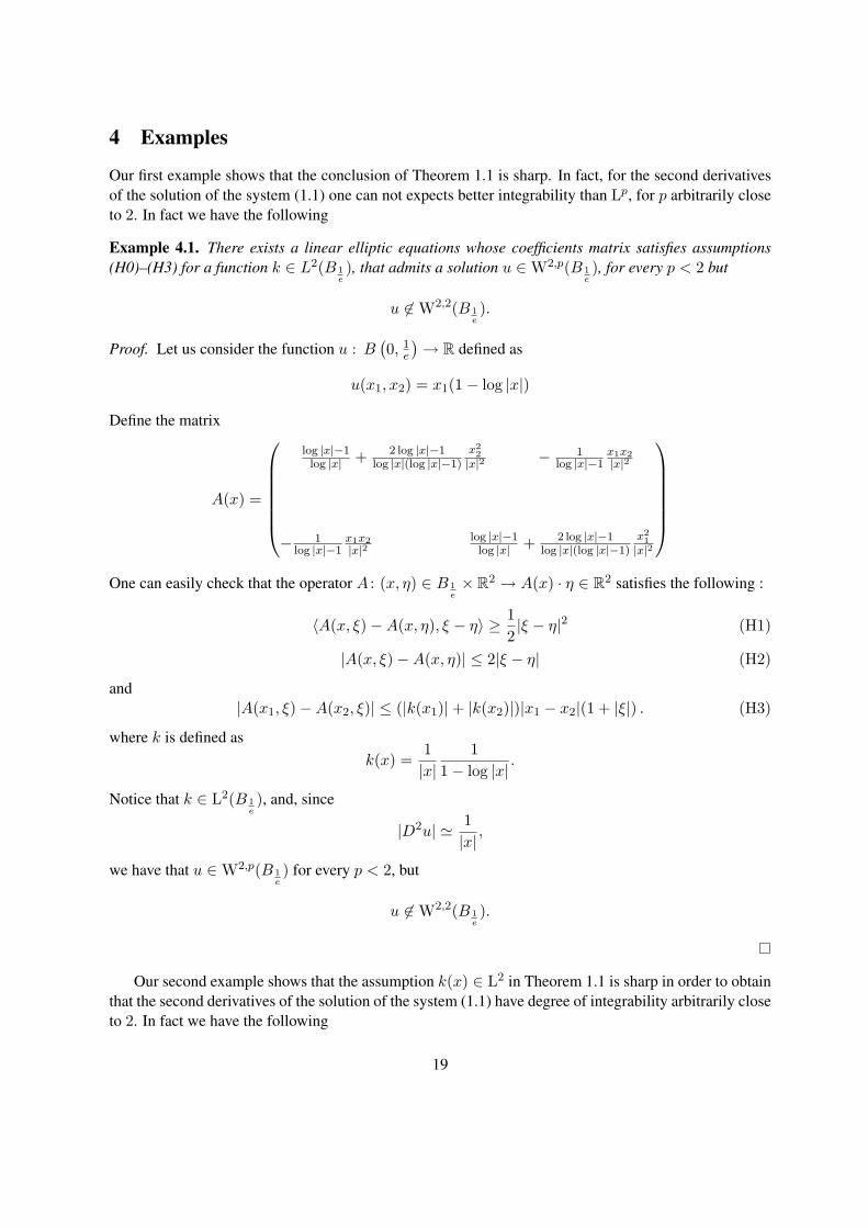
Our first example shows that the conclusion of Theorem 1.1 is sharp. In fact, for the second derivativesof the solution of the system (1.1) one can not expects better integrability than Lp, for p arbitrarily closeto 2. In fact we have the following
Example 4.1. There exists a linear elliptic equations whose coefficients matrix satisfies assumptions(H0)–(H3) for a function k ∈ L2(B 1
e), that admits a solution u ∈W2,p(B 1
e), for every p < 2 but
u 6∈W2,2(B 1e).
Proof. Let us consider the function u : B(0, 1
e
)→ R defined as
u(x1, x2) = x1(1− log |x|)
Define the matrix
A(x) =
log |x|−1log |x| + 2 log |x|−1
log |x|(log |x|−1)x22|x|2 − 1
log |x|−1x1x2|x|2
− 1log |x|−1
x1x2|x|2
log |x|−1log |x| + 2 log |x|−1
log |x|(log |x|−1)x21|x|2
One can easily check that the operator A : (x, η) ∈ B 1
e× R2 → A(x) · η ∈ R2 satisfies the following :
〈A(x, ξ)−A(x, η), ξ − η〉 ≥ 12|ξ − η|2 (H1)
|A(x, ξ)−A(x, η)| ≤ 2|ξ − η| (H2)
and|A(x1, ξ)−A(x2, ξ)| ≤ (|k(x1)|+ |k(x2)|)|x1 − x2|(1 + |ξ|) . (H3)
where k is defined ask(x) =
1|x|
11− log |x|
.
Notice that k ∈ L2(B 1e), and, since
|D2u| ' 1|x|,
we have that u ∈W2,p(B 1e) for every p < 2, but
u 6∈W2,2(B 1e).
Our second example shows that the assumption k(x) ∈ L2 in Theorem 1.1 is sharp in order to obtainthat the second derivatives of the solution of the system (1.1) have degree of integrability arbitrarily closeto 2. In fact we have the following
19
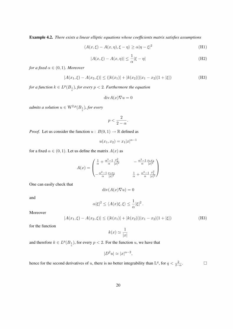
Example 4.2. There exists a linear elliptic equations whose coefficients matrix satisfies assumptions
〈A(x, ξ)−A(x, η), ξ − η〉 ≥ α|η − ξ|2 (H1)
|A(x, ξ)−A(x, η)| ≤ 1α|ξ − η| (H2)
for a fixed α ∈ (0, 1). Moreover
|A(x1, ξ)−A(x2, ξ)| ≤ (|k(x1)|+ |k(x2)|)|x1 − x2|(1 + |ξ|) (H3)
for a function k ∈ Lp(B 1e), for every p < 2. Furthermore the equation
divA(x)∇u = 0
admits a solution u ∈W2,p(B 1e), for every
p <2
2− α.
Proof. Let us consider the function u : B(0, 1)→ R defined as
u(x1, x2) = x1|x|α−1
for a fixed α ∈ (0, 1). Let us define the matrix A(x) as
A(x) =
1α + α2−1
αx22|x|2 − α2−1
αx1x2|x|2
−α2−1α
x1x2|x|2
1α + α2−1
αx21|x|2
One can easily check that
div(A(x)∇u) = 0
andα|ξ|2 ≤ 〈A(x)ξ, ξ〉 ≤ 1
α|ξ|2 .
Moreover|A(x1, ξ)−A(x2, ξ)| ≤ (|k(x1)|+ |k(x2)|)|x1 − x2|(1 + |ξ|) (H3)
for the functionk(x) ' 1
|x|
and therefore k ∈ Lp(B 1e), for every p < 2. For the function u, we have that
|D2u| ' |x|α−2,
hence for the second derivatives of u, there is no better integrability than Lq, for q < 22−α .
20
References
[1] E. Acerbi and N. Fusco. Partial regularity under anisotropic (p, q) growth conditions. J. Diff. Eq.107 (1994), 46–67.
[2] M. Bildhauer. Convex variational problems. Linear, nearly linear and anisotropic growth condi-tions. Lecture Notes in Mathematics, 1818. Springer-Verlag, Berlin, 2003.
[3] Boccardo, L. and Gallouet, T., Nonlinear elliptic equations with right hand side measures. Comm.Part. Diff. Equ. 17 (1992)(3–4), 641 – 655.
[4] V. Bogelein, F. Duzaar, J. Habermann and C. Scheven. Partial Holder continuity for discontinuouselliptic problems with VMO-coefficients, Proc. London Math. Soc. (2011), 1–34.
[5] M. Carozza, J. Kristensen and A. Passarelli di Napoli . Higher differentiability of minimizers ofconvex variational integrals. Ann. Inst. H. Poincare Anal. Non Lineaire 28 (2011), no. 3, 395–411.
[6] A. Cianchi and L. Pick. Sobolev embeddings into BMO, VMO and L∞, Ark. Mat. 36 (1998), 319–340
[7] A. Clop, D. Faraco, J. Mateu, J. Orobitg and X. Zhong. Beltrami equations with coefficient in theSobolev space W 1,p, Publ. Mat. 53 (2009), no. 1, 197–230.
[8] B. De Maria and A. Passarelli di Napoli Partial regularity for non autonomous functionals with nonstandard growth conditions. Calc. Var. Partial Differential Equations 38 (2010), no. 3–4, 417–439.
[9] B. De Maria and A. Passarelli di Napoli A new partial regularity result for non-autonomous convexintegrals with non-standard growth conditions. J. Differential Equations 250 (2011), no. 3, 1363–1385.
[10] F. Duzaar, A. Gastel and J.F. Grotowski. Partial regularity for almost minimizers of quasiconvexintegrals. SIAM J. Math. Anal. 32 (2000), 665–687.
[11] F. Duzaar and M. Krontz. Regularity of ω- minimizers of quasiconvex integrals. Diff. Geom. Appl.17 (2002), 139–152.
[12] L. Esposito, F. Leonetti and G. Mingione. Regularity for minimizers of functionals with p−q growth.NoDEA, Nonlinear Differ. Eq. Appl. 6 (1999), 133–148.
[13] L. Esposito, F. Leonetti and G. Mingione. Sharp regularity for functionals with (p, q) growth. J. Dif-ferential Equations 204 (2004), no. 1, 5–55.
[14] M. Foss and G.R. Mingione. Partial continuity for elliptic problems Ann. I. H. Poincare AN 25(2008), 471–503
[15] F. Giannetti, L. Greco and A. Passarelli di Napoli. Regularity of solutions of degenerate A-harmonicequations, Nonlinear Anal. 73 (2010), 2651–2665.
[16] F. Giannetti and A. Passarelli di Napoli. On very weak solutions of degenerate p-harmonic equa-tions. NoDEA, Nonlinear Differ. Equ. Appl. 14 (2007), 739–751
21
[17] M. Giaquinta. Multiple integrals in the calculus of variations and nonlinear elliptic systems. Annalsof Math. Studies 105, Princeton Univ. Press, 1983.
[18] E. Giusti. Direct methods in the calculus of variations. World Scientific, 2003.
[19] J. Kristensen and C. Melcher. Regularity in oscillatory nonlinear elliptic systems. Math. Z. 260(2008), 813–847.
[20] J. Kristensen and G. Mingione. Boundary regularity in variational problems. Arch. Ra-tion. Mech. Anal. 198 (2010), 369–455.
[21] T. Iwaniec and C. Sbordone, Weak minima of variational integrals. J. Reine Angew. Math. 454(1994), 143-161.
[22] P. Marcellini. Regularity of minimizers of integrals of the calculus of variations with non-standardgrowth conditions. Arch. Ration. Mech. Anal. 105 (1989), 267–284.
[23] P. Marcellini. Regularity and existence of solutions of elliptic equations with (p, q) growth condi-tions. J. Diff. Eq. 90 (1991), 1–30.
[24] P. Marcellini. Everywhere regularity for a class of elliptic systems without growth conditions.Ann. Scuola Normale Sup. Pisa, Cl. Sci. 23 (1996), 1–25.
[25] A. Passarelli di Napoli . Higher differentiability of minimizers of variational integrals with Sobolevcoefficients. Adv. Cal. Var. (2012).
[26] A. Passarelli di Napoli and F. Siepe. A regularity result for a class of anisotropic systems.Rend. Ist. Mat di Trieste (1997), 13–31.
[27] D. Percivale Continuity of solutions of a class of linear non uniformly elliptic equations. RicercheMat. 48 (1999), no. 2, 249–258 (2000).
[28] W.P. Ziemer. Weakly differentiable functions. Graduate Texts in Maths. 120, Springer-Verlag, 1989.
Universita di Napoli ”Federico II”Dipartimento di Mat. e Appl. ”R. Caccioppoli”,Via Cintia, 80126 Napoli, ItalyE-mail address: [email protected]
22


![Modules over the noncommutative torus, elliptic curves …wpage.unina.it/francesco.dandrea/Files/HIM14.[slides].pdf · Modules over the noncommutative torus, elliptic curves and cochain](https://static.fdocument.org/doc/165x107/5b9ef74409d3f2d0208c7863/modules-over-the-noncommutative-torus-elliptic-curves-wpageuninait-slidespdf.jpg)