Stochastic Homogenization For Elliptic NonlocalEquations... And Beyond

(Ginzburg-Landau equations, Dislocations andHomogenization– Ile de Re, May 2011)

Russell Schwab

Carnegie Mellon University

26 May, 2011

thanks

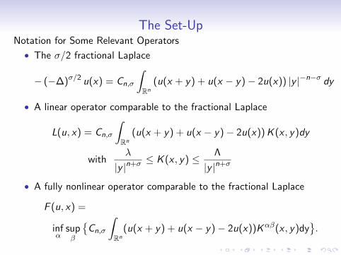
The Set-UpNotation for Some Relevant Operators

• The σ/2 fractional Laplace

− (−∆)σ/2 u(x) = Cn,σ

∫Rn

(u(x + y) + u(x − y)− 2u(x)) |y |−n−σ dy

• A linear operator comparable to the fractional Laplace

L(u, x) = Cn,σ

∫Rn

(u(x + y) + u(x − y)− 2u(x)) K (x , y)dy

withλ

|y |n+σ≤ K (x , y) ≤ Λ

|y |n+σ

• A fully nonlinear operator comparable to the fractional Laplace

F (u, x) =

infα

supβ

Cn,σ

∫Rn

(u(x + y) + u(x − y)− 2u(x))Kαβ(x , y)dy.

quick comments

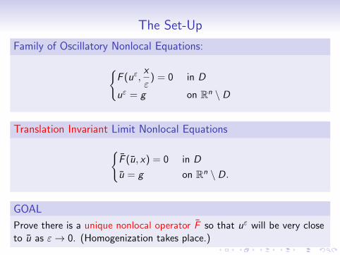
The Set-Up

Family of Oscillatory Nonlocal Equations:

F (uε,

x

ε, ω) = 0 in D

uε = g on Rn \ D

F (u,x

ε, ω) =

infα

supβ

f αβ(

x

ε, ω) + Cn,σ

∫Rn

(u(x + y) + u(x − y)− 2u(x))Kαβ(x

ε, y , ω)dy

.(

Think of a more familiar 2nd order equation:

F (D2u,x

ε) = inf

αsupβ

f αβ(

x

ε) + aαβij (

x

ε)uxixj (x)

)

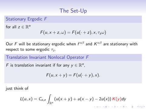
The Set-Up

Stationary Ergodic F

for all z ∈ Rn

F (u, x + z , ω) = F (u(·+ z), x , τzω)

Our F will be stationary ergodic when f αβ and Kαβ are stationary withrespect to some ergodic τz .

Translation Invariant Nonlocal Operator F

F is translation invariant if for any y ∈ Rn,

F (u, x + y) = F (u(·+ y), x).

just think of

L(u, x) = Cn,σ

∫Rn

(u(x + y) + u(x − y)− 2u(x)) K (y)dy

The Set-Up

Family of Oscillatory Nonlocal Equations:

F (uε,

x

ε) = 0 in D

uε = g on Rn \ D

Translation Invariant Limit Nonlocal Equations

F (u, x) = 0 in D

u = g on Rn \ D.

GOAL

Prove there is a unique nonlocal operator F so that uε will be very closeto u as ε→ 0. (Homogenization takes place.)

The Set-Up

picture of εXε−σt in random environment.

The Set-Up

Which is more important, “integro” intuition or “differential” intuition???

Main Theorem

Theorem (Stochastic Homogenization of Nonlocal Equations–preprint at arXiv.org)

If F is stationary ergodic and uniformly elliptic, plus technicalassumptions, then there exists a translation invariant elliptic nonlocaloperator F with the same ellipticity as F , such that for a.e. ω uε(ω)→ ulocally uniformly and u is the unique solution of

F (u, x) = 0 in D

u = g on Rn \ D.

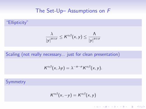
The Set-Up– Assumptions on F

“Ellipticity”

λ

|y |n+σ≤ Kαβ(x , y) ≤ Λ

|y |n+σ

Scaling (not really necessary... just for clean presentation)

Kαβ(x , λy) = λ−n−σKαβ(x , y).

Symmetry

Kαβ(x ,−y) = Kαβ(x , y)

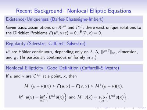
Recent Background– Nonlocal Elliptic Equations

Existence/Uniqueness (Barles-Chasseigne-Imbert)

Given basic assumptions on Kαβ and f αβ, there exist unique solutions tothe Dirichlet Problems F (uε, x/ε) = 0, F (u, x) = 0.

Regularity (Silvestre, Caffarelli-Silvestre)

uε are Holder continuous, depending only on λ, Λ, ‖f αβ‖∞, dimension,and g . (In particular, continuous uniformly in ε.)

Nonlocal Ellipticity– Good Definition (Caffarelli-Silvestre)

If u and v are C 1,1 at a point, x , then

M−(u − v)(x) ≤ F (u, x)− F (v , x) ≤ M+(u − v)(x).

M−u(x) = infαβ

Lαβu(x)

and M+u(x) = sup

αβ

Lαβu(x)

.

Historical Homogenization Background

• De Giorgi, Jikov, Kozlov, Murat, Spagnolo, Tartar, Yurinskii, ...many many more

• Bensoussan-Lions-Papanicolaou 1978– Asymptotic analysis forperiodic structures

• Papanicolaou-Varadhan– Random Homogenization Linear EllipticOperators

• Lions-Papanicolaou-Varadhan (unpublished)– PeriodicHomogenization of Hamilton-Jacobi Equations

• Evans 1992– Periodic Homogenization of Fully Nonlinear PDEs

• Arisawa-Lions 1998– On Ergodic Stochastic Control

• Caffarelli-Souganidis-Wang 2005– Stochastic Homogenization OfFully Nonlinear Elliptic Equations

• (related results) Arisawa 2009– Homogenization of a Class ofIntegro-Differential Equations with Levy Operators

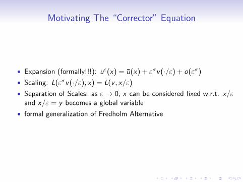
Motivating The “Corrector” Equation

• Expansion (formally!!!): uε(x) = u(x) + εσv(·/ε) + o(εσ)

• Scaling: L(εσv(·/ε), x) = L(v , x/ε)

• Separation of Scales: as ε→ 0, x can be considered fixed w.r.t. x/εand x/ε = y becomes a global variable

• formal generalization of Fredholm Alternative

Motivating The “Corrector” EquationJust for the fractional Laplace sufficient for the idea...

−(−∆)σ/2uε = f (x

ε)

• Plug Expansion into equation plus scaling:

−(−∆)σ/2u(x) +−(−∆)σ/2v(x

ε) = f (

x

ε)

• Global variables:

−(−∆)σ/2u(x) +−(−∆)σ/2v(y) = f (y) + F

• Need to find such a v : Fredholm says only if

F +

∫Q1

fdy − (−(−∆)σ/2u(x)) = 0

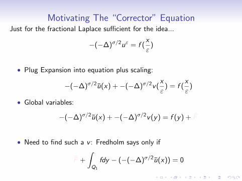
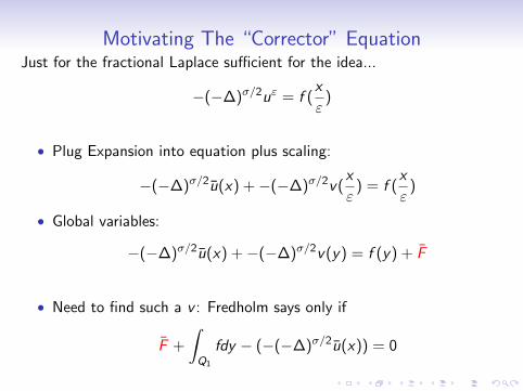
Motivating The “Corrector” EquationJust for the fractional Laplace sufficient for the idea...

−(−∆)σ/2uε = f (x

ε)

• Plug Expansion into equation plus scaling:

−(−∆)σ/2u(x) +−(−∆)σ/2v(x

ε) = f (

x

ε)

• Global variables:

−(−∆)σ/2u(x) +−(−∆)σ/2v(y) = f (y) + F

• Need to find such a v : Fredholm says only if

F +

∫Q1

fdy − (−(−∆)σ/2u(x)) = 0

Motivating The “Corrector” EquationRestate what we just did...

True Corrector... Special Case

For all u and x fixed, there exists a unique constant, F , such that thereis a bounded periodic periodic solution of

(−(−∆)σ/2u(x))− (−∆)σ/2v(y) = f (y) + F (u, x)

Formal Solution To Homogenization

−(−∆)σ/2u(x) +−(−∆)σ/2v(x

ε) = f (

x

ε)

which reads, after ε→ 0,F (u, x) = 0

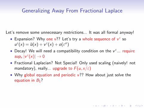
Generalizing Away From Fractional Laplace

Let’s remove some unnecessary restrictions... It was all formal anyway!

• Expansion? Why one v?? Let’s try a whole sequence of v ε souε(x) = u(x) + v ε(x) + o(εσ)

• Decay! We will need a compatibility condition on the v ε... requiresupx |v ε(x)| → 0

• Fractional Laplacian? Not Special! Only used scaling (naively! notmandatory), really... upgrade to F (u, x/ε)

• Why global equation and periodic v?? How about just solve theequation in B1?

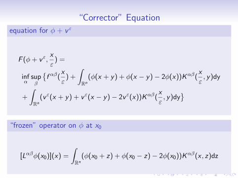
“Corrector” Equation

equation for φ + v ε

F (φ+ v ε,x

ε) =

infα

supβ

f αβ(

x

ε) +

∫Rn

(φ(x + y) + φ(x − y)− 2φ(x))Kαβ(x

ε, y)dy

+

∫Rn

(v ε(x + y) + v ε(x − y)− 2v ε(x))Kαβ(x

ε, y)dy

“frozen” operator on φ at x0

[Lαβφ(x0)](x) =

∫Rn

(φ(x0 + z) + φ(x0 − z)− 2φ(x0))Kαβ(x , z)dz

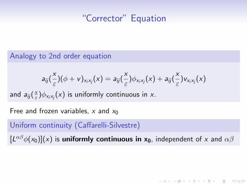
“Corrector” Equation

Analogy to 2nd order equation

aij(x

ε)(φ+ v)xixj (x) = aij(

x

ε)φxixj (x) + aij(

x

ε)vxixj (x)

and aij(xε )φxixj (x) is uniformly continuous in x .

Free and frozen variables, x and x0

Uniform continuity (Caffarelli-Silvestre)

[Lαβφ(x0)](x) is uniformly continuous in x0, independent of x and αβ

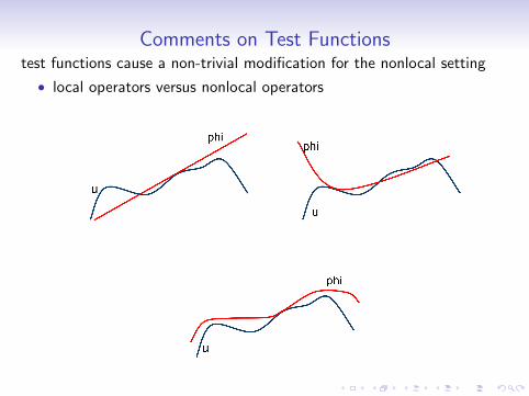
Comments on Test Functionstest functions cause a non-trivial modification for the nonlocal setting

• local operators versus nonlocal operators

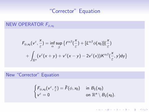
“Corrector” Equation

NEW OPERATOR Fφ,x0

Fφ,x0(v ε,x

ε) = inf

αsupβ

f αβ(

x

ε) + [Lαβφ(x0)](

x

ε)

+

∫Rn

(v ε(x + y) + v ε(x − y)− 2v ε(x))Kαβ(x

ε, y)dy

New “Corrector” Equation

Fφ,x0(v ε, xε ) = F (φ, x0) in B1(x0)

v ε = 0 on Rn \ B1(x0).

“Corrector” Equation

Proposition (“Corrector” Equation)

For all smooth φ and x0 fixed, there exists a set of full measure Ωφ,x0 anda unique choice for the value of F (φ, x0) such that for ω ∈ Ωφ,x0 , thesolutions of the “corrector” equation also satisfy

limε→0

maxB1(x0)

|v ε| = 0.

(via the perturbed test function method, this proposition is equivalent tohomogenization)

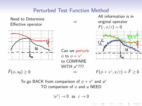
Perturbed Test Function Method

Need to DetermineEffective operator

⇒All information is inoriginal operatorF (·, x/ε) = 0

Can we perturbφ to φ+ v ε

to COMPAREWITH uε???

F (φ, x0) ≥ 0 ⇒ F (φ+ v ε, x/ε) = F ≥ 0

To go BACK from comparison of φ+ v ε and uε

TO comparison of φ and u NEED

|v ε| → 0 as ε→ 0

Finding F ... Variational Problem

(Caffarelli-Sougandis-Wang... *In spirit)

Consider a generic choice of a Right Hand Side, l is fixed

Fφ,x0(v εl ,

xε ) = l in B1(x0)

v εl = 0 on Rn \ B1(x0).

How does the choice of l affect the decay of v εl ?

decay property

limε→0 maxB1(x0) |v ε| = 0 ⇐⇒ (v εl )∗ = (v εl )∗ = 0

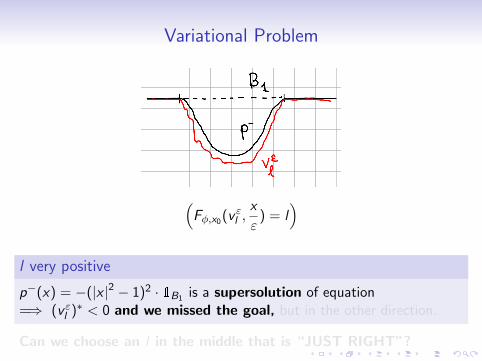
Variational Problem

l very negative

p+(x) = (1− |x |2)2 · 1B1 is a subsolution of equation=⇒ (v εl )∗ > 0 and we missed the goal.

(Fφ,x0(v εl ,

x

ε) = l

)

Variational Problem

(Fφ,x0(v εl ,

x

ε) = l

)l very positive

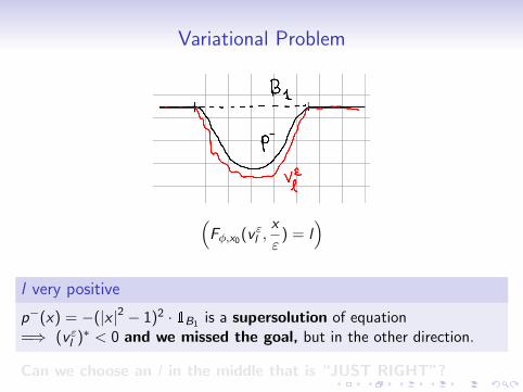
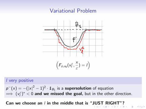
p−(x) = −(|x |2 − 1)2 · 1B1 is a supersolution of equation=⇒ (v εl )∗ < 0 and we missed the goal, but in the other direction.

Can we choose an l in the middle that is “JUST RIGHT”?

Variational Problem

(Fφ,x0(v εl ,

x

ε) = l

)l very positive

p−(x) = −(|x |2 − 1)2 · 1B1 is a supersolution of equation=⇒ (v εl )∗ < 0 and we missed the goal, but in the other direction.

Can we choose an l in the middle that is “JUST RIGHT”?

Variational Problem

(Fφ,x0(v εl ,

x

ε) = l

)l very positive

p−(x) = −(|x |2 − 1)2 · 1B1 is a supersolution of equation=⇒ (v εl )∗ < 0 and we missed the goal, but in the other direction.

Can we choose an l in the middle that is “JUST RIGHT”?

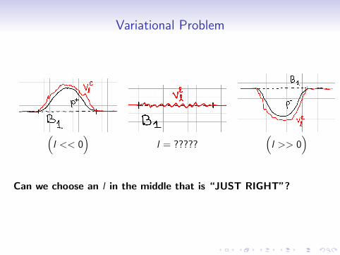
Variational Problem

(l << 0

)l = ?????

(l >> 0

)

Can we choose an l in the middle that is “JUST RIGHT”?

Obstacle Problem

(Caffarelli-Sougandis-Wang) The answer is YES.

Information From Obstacle Problem

The obstacle problem gives relationship between the choice of l and thedecay of v εl .

Obstacle Problem

The Solution of The Obstacle Problem In a Set A

U lA = inf

u : Fφ,x0(u, y) ≤ l in A and u ≥ 0 in Rn

equation: U l

A is the least supersolution of Fφ,x0 = l in A

obstacle: U lA must be above the obstacle which is 0 in all of Rn

Lemma (Holder Continuity)

U lA is γ-Holder Continuous depending only on λ, Λ, ‖f αβ‖∞, φ,

dimension, and A.

Monotonicity and Stationarity of Obstacle Problem

If A ⊂ B, then U lA ≤ U l

B . For z ∈ Rn, U lA+z(x , ω) = U l

A(x − z , τzω)

Obstacle Problem

The Solution of The Obstacle Problem In a Set A

U lA = inf

u : Fφ,x0(u, y) ≤ l in A and u ≥ 0 in Rn

equation: U l

A is the least supersolution of Fφ,x0 = l in A

obstacle: U lA must be above the obstacle which is 0 in all of Rn

Lemma (Holder Continuity)

U lA is γ-Holder Continuous depending only on λ, Λ, ‖f αβ‖∞, φ,

dimension, and A.

Monotonicity and Stationarity of Obstacle Problem

If A ⊂ B, then U lA ≤ U l

B . For z ∈ Rn, U lA+z(x , ω) = U l

A(x − z , τzω)

Obstacle Problem

NOTATION

Rescaled Solution

uε,l = inf

u : Fφ,x0(u,y

ε) ≤ l in Q1 and u ≥ 0 in Rn

.

Solution in Q1 and Solution in Q1/ε

uε,l(x) = εσU lQ1/ε

(x

ε)

Contact Set

Kε = U lQ1/ε

= 0 and kε = uε,l = 0

Obstacle Problem- Relationship to v εlEquation for uε,l

Fφ,x0(uε,l ,x

ε) ≤ C (F )1kε + l and uε,l = 0 in Rn \ Q1

Equation for uε,l − v εl

M−(uε,l − v εl ) ≤ Fφ,x0(uε,l ,x

ε)− Fφ,x0(v εl ,

x

ε) ≤ C (F )1kε

Obstacle Problem- Contact Limits

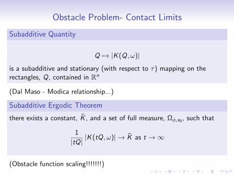
Subadditive Quantity

Q 7→ |K (Q, ω)|

is a subadditive and stationary (with respect to τ) mapping on therectangles, Q, contained in Rn

(Dal Maso - Modica relationship...)

Subadditive Ergodic Theorem

there exists a constant, K , and a set of full measure, Ωφ,x0 , such that

1

|tQ||K (tQ, ω)| → K as t →∞

(Obstacle function scaling!!!!!!!)

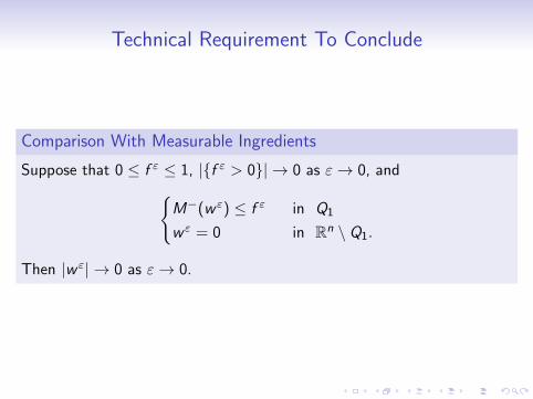
Technical Requirement To Conclude

Comparison With Measurable Ingredients

Suppose that 0 ≤ f ε ≤ 1, |f ε > 0| → 0 as ε→ 0, andM−(w ε) ≤ f ε in Q1

w ε = 0 in Rn \ Q1.

Then |w ε| → 0 as ε→ 0.

Conclusion of “Corrector” Equation

K characterizes limits of v εl

if K > 0, then (v εl )∗ ≤ 0 and if K = 0 then (v ε)∗ ≥ 0

The Good Choice of F

F (φ, x0) = sup

l : K = 0

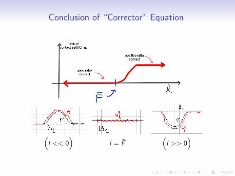
Conclusion of “Corrector” Equation

(l << 0

)l = F

(l >> 0

)

A Very Basic QuestionWhen does comparison with measurable ingredients hold? Even forLINEAR EQUATIONS!

Equations with measurable ingredients (supersolutions)

Lw ε ≤ f ε in Q1

w ε = 0 in Rn \ Q1.

Lw(x) =

∫(w(x + y) + w(x − y)− 2w(x))K (x , y)dy

(K bounded measurable, comparable to |y |−n−σ)

limit as |f ε > 0| → 0????? (simplest case 0 ≤ f ε ≤ 1)

‖w ε‖∞ → 0??????

A Very Basic Question

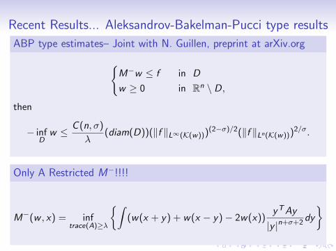
Recent Results... Aleksandrov-Bakelman-Pucci type results

ABP type estimates– Joint with N. Guillen, preprint at arXiv.org

M−w ≤ f in D

w ≥ 0 in Rn \ D,

then

− infD

w ≤ C (n, σ)

λ(diam(D))(‖f ‖L∞(K(w)))

(2−σ)/2(‖f ‖Ln(K(w)))2/σ.

Only A Restricted M−!!!!

M−(w , x) = inftrace(A)≥λ

∫(w(x + y) + w(x − y)− 2w(x))

yTAy

|y |n+σ+2dy

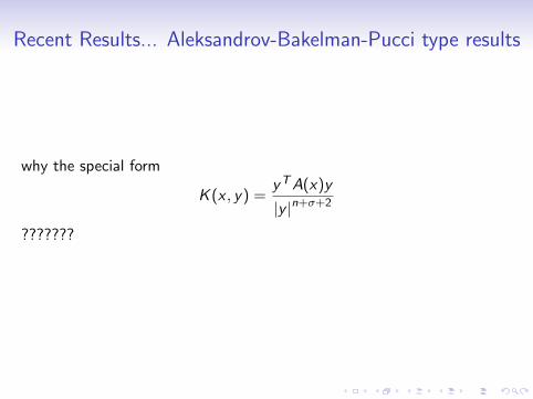
Recent Results... Aleksandrov-Bakelman-Pucci type results

why the special form

K (x , y) =yTA(x)y

|y |n+σ+2

???????

Thank You!

M. Arisawa and P.-L. Lions. On ergodic stochastic control. Comm.Partial Differential Equations, 23(11-12):2187–2217, 1998.

Mariko Arisawa. Homogenization of a class of integro-differentialequations with Levy operators. Comm. Partial Differential Equations,34(7-9):617–624, 2009.

G. Barles, E. Chasseigne, and C. Imbert. On the dirichlet problem forsecond-order elliptic integro-differential equations. Indiana Univ.Math. J., 57(1):213–246, 2008.

Guy Barles and Cyril Imbert. Second-order elliptic integro-differentialequations: viscosity solutions’ theory revisited. Ann. Inst. H.Poincare Anal. Non Lineaire, 25(3):567–585, 2008.

Alain Bensoussan, Jacques-Louis Lions, and George Papanicolaou.Asymptotic analysis for periodic structures, volume 5 of Studies inMathematics and its Applications. North-Holland Publishing Co.,Amsterdam, 1978.

L. A. Caffarelli and L. Silvestre. The Evans-Krylov theorem for nonlocal fully non linear equations. Ann. of Math. (2), To Appear.

Luis A. Caffarelli, Panagiotis E. Souganidis, and L. Wang.Homogenization of fully nonlinear, uniformly elliptic and parabolicpartial differential equations in stationary ergodic media. Comm.Pure Appl. Math., 58(3):319–361, 2005.

Lawrence C. Evans. Periodic homogenisation of certain fullynonlinear partial differential equations. Proc. Roy. Soc. EdinburghSect. A, 120(3-4):245–265, 1992.

Russell W. Schwab. Periodic homogenization for nonlinearintegro-differential equations. SIAM J. Math. Analysis, to appear.