1

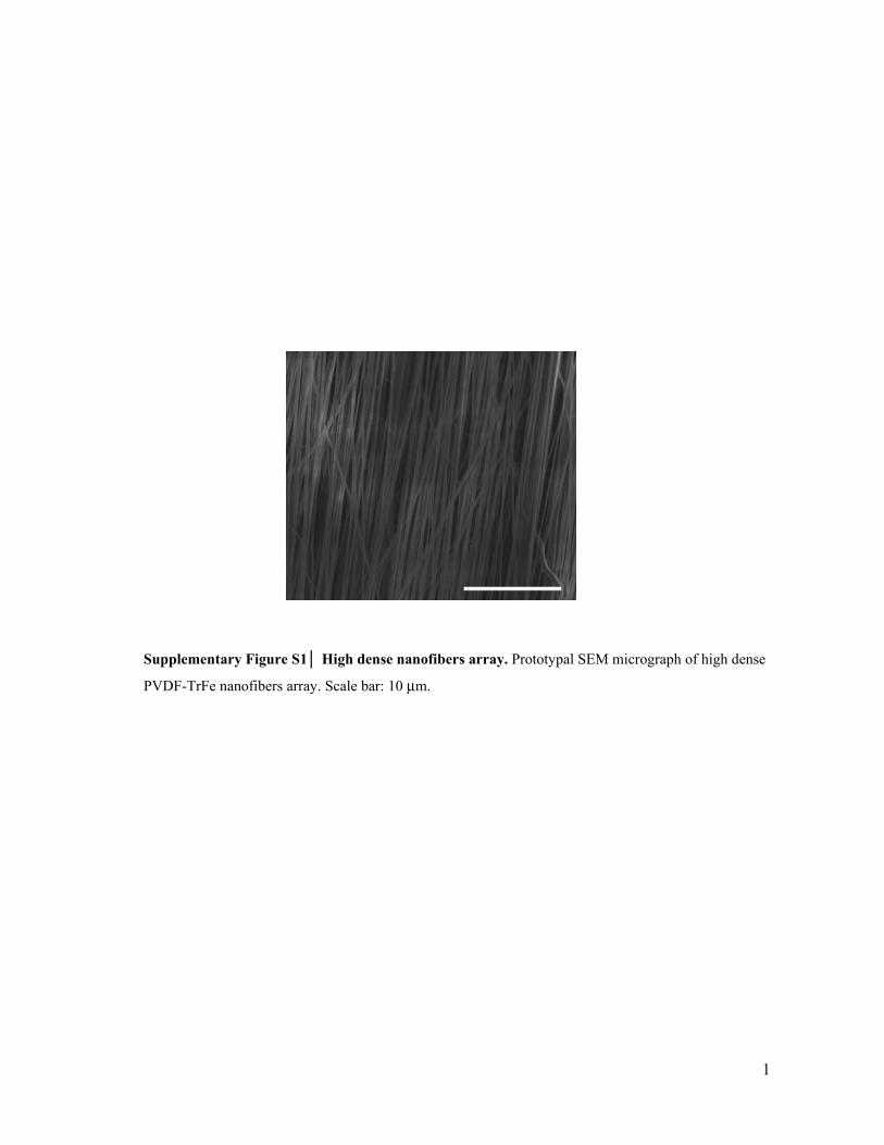
Supplementary Figure S1│ High dense nanofibers array. Prototypal SEM micrograph of high dense

PVDF-TrFe nanofibers array. Scale bar: 10 μm.

2

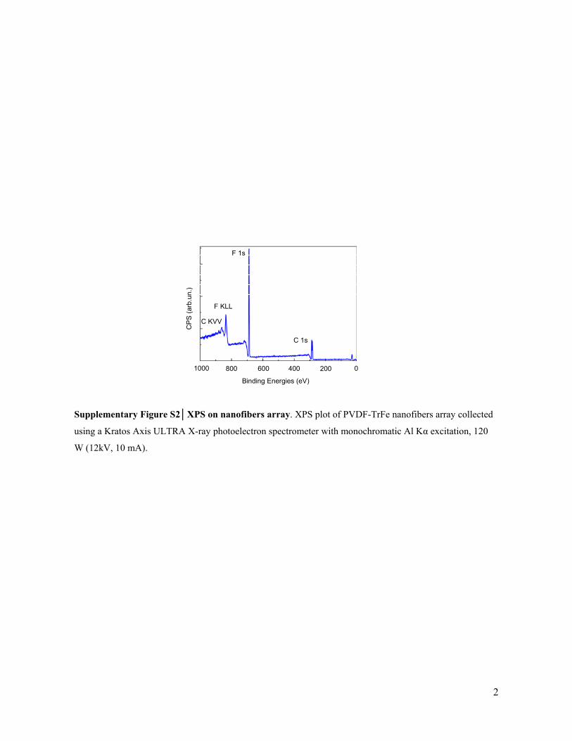
Supplementary Figure S2│XPS on nanofibers array. XPS plot of PVDF-TrFe nanofibers array collected

using a Kratos Axis ULTRA X-ray photoelectron spectrometer with monochromatic Al Kα excitation, 120

W (12kV, 10 mA).

1000 800 600 400 200 0

Binding Energies (eV)

CP

S (

arb.

un.)

C KVV

F KLL

F 1s

C 1s

3

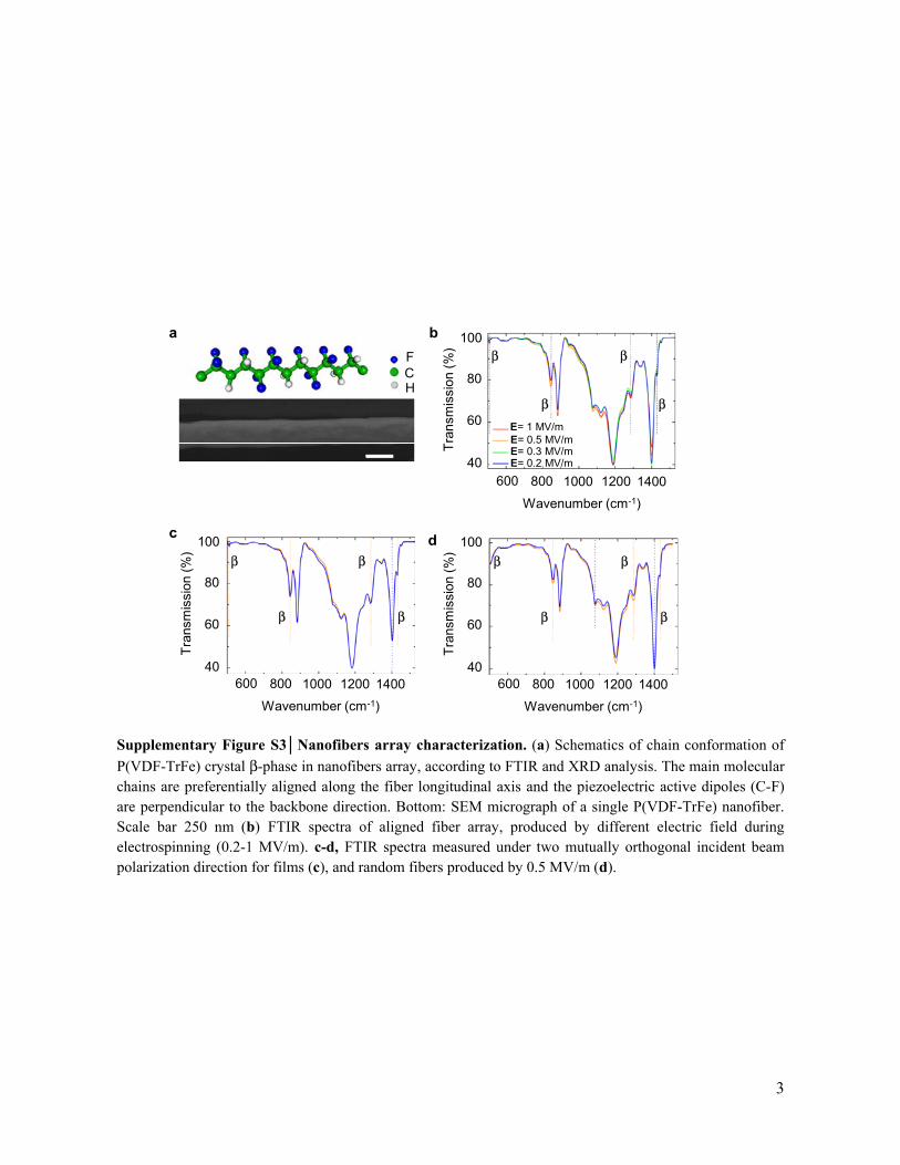
Supplementary Figure S3│Nanofibers array characterization. (a) Schematics of chain conformation of

P(VDF-TrFe) crystal β-phase in nanofibers array, according to FTIR and XRD analysis. The main molecular chains are preferentially aligned along the fiber longitudinal axis and the piezoelectric active dipoles (C-F) are perpendicular to the backbone direction. Bottom: SEM micrograph of a single P(VDF-TrFe) nanofiber. Scale bar 250 nm (b) FTIR spectra of aligned fiber array, produced by different electric field during electrospinning (0.2-1 MV/m). c-d, FTIR spectra measured under two mutually orthogonal incident beam polarization direction for films (c), and random fibers produced by 0.5 MV/m (d).

E= 1 MV/mE= 0.5 MV/m

E= 0.2 MV/mE= 0.3 MV/m

600 800 1000 1200 1400

100

80

60

40

Wavenumber (cm-1)

Tra

nsm

issi

on (

%) β

β

β

β

FCH

600 800 1000 1200 1400

100

80

60

40

Wavenumber (cm-1)

Tra

nsm

issi

on (

%)

β

β

β

β

600 800 1000 1200 1400

100

80

60

40

Wavenumber (cm-1)

Tra

nsm

issi

on (

%)

β

β

β

β

a

c

b

d

4

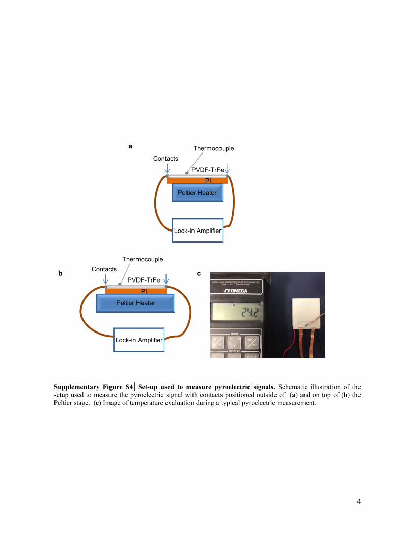
Supplementary Figure S4│Set-up used to measure pyroelectric signals. Schematic illustration of the setup used to measure the pyroelectric signal with contacts positioned outside of (a) and on top of (b) the Peltier stage. (c) Image of temperature evaluation during a typical pyroelectric measurement.

Contacts

Lock-in Amplifier

Lock-in Amplifier

Peltier Heater

Thermocouple

Peltier Heater

Thermocouple

Contacts

PI

PI

PVDF-TrFe

a

b cPVDF-TrFe

5

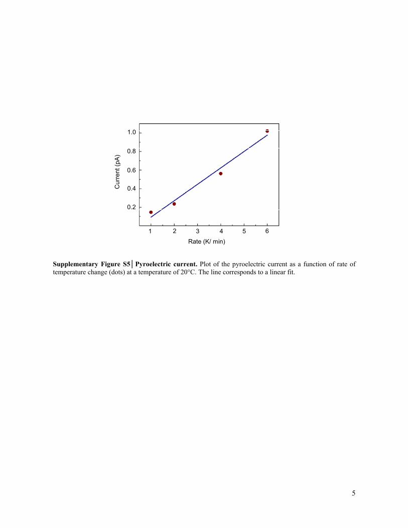
Supplementary Figure S5│Pyroelectric current. Plot of the pyroelectric current as a function of rate of temperature change (dots) at a temperature of 20°C. The line corresponds to a linear fit.

Rate (K/ min)

Cur

rent

(pA

)

1 2 3 4 5 6

0.2

0.4

0.6

0.8

1.0

6

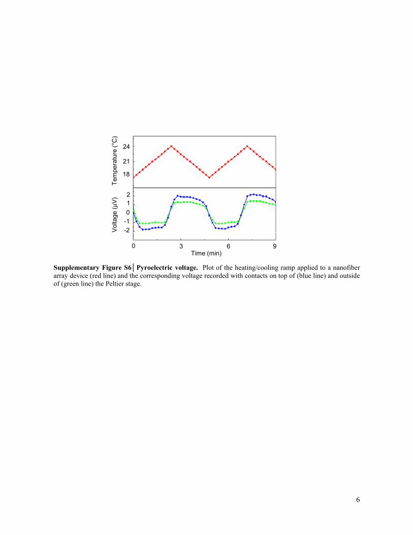
Supplementary Figure S6│Pyroelectric voltage. Plot of the heating/cooling ramp applied to a nanofiber array device (red line) and the corresponding voltage recorded with contacts on top of (blue line) and outside of (green line) the Peltier stage.

Time (min)

Vol

tage

(μV

)T

empe

ratu

re (

°C)

18

21

24

1

0

-1

0 3 6 9

2

-2

7

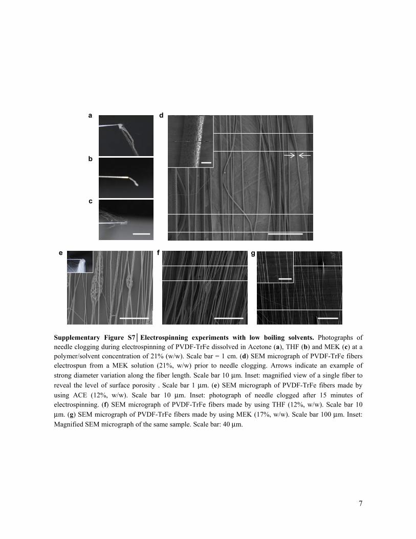
Supplementary Figure S7│Electrospinning experiments with low boiling solvents. Photographs of needle clogging during electrospinning of PVDF-TrFe dissolved in Acetone (a), THF (b) and MEK (c) at a polymer/solvent concentration of 21% (w/w). Scale bar = 1 cm. (d) SEM micrograph of PVDF-TrFe fibers electrospun from a MEK solution (21%, w/w) prior to needle clogging. Arrows indicate an example of

strong diameter variation along the fiber length. Scale bar 10 μm. Inset: magnified view of a single fiber to

reveal the level of surface porosity . Scale bar 1 μm. (e) SEM micrograph of PVDF-TrFe fibers made by

using ACE (12%, w/w). Scale bar 10 μm. Inset: photograph of needle clogged after 15 minutes of electrospinning. (f) SEM micrograph of PVDF-TrFe fibers made by using THF (12%, w/w). Scale bar 10

μm. (g) SEM micrograph of PVDF-TrFe fibers made by using MEK (17%, w/w). Scale bar 100 μm. Inset:

Magnified SEM micrograph of the same sample. Scale bar: 40 μm.

a

b

c

d

e f g

8

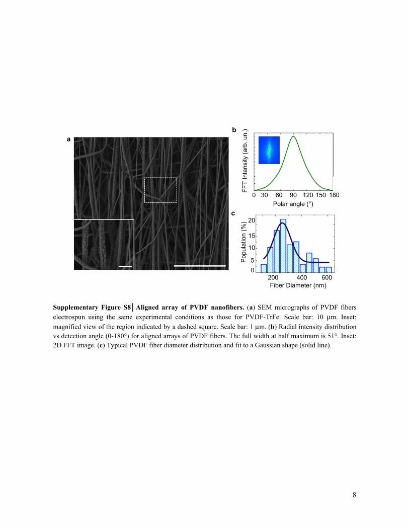
Supplementary Figure S8│Aligned array of PVDF nanofibers. (a) SEM micrographs of PVDF fibers

electrospun using the same experimental conditions as those for PVDF-TrFe. Scale bar: 10 μm. Inset:

magnified view of the region indicated by a dashed square. Scale bar: 1 μm. (b) Radial intensity distribution vs detection angle (0-180°) for aligned arrays of PVDF fibers. The full width at half maximum is 51°. Inset: 2D FFT image. (c) Typical PVDF fiber diameter distribution and fit to a Gaussian shape (solid line).

1800 30 60 90 120 150

FF

T In

tens

ity(a

rb. u

n.)

Polar angle (°)

200 6000

10

5

15P

opul

atio

n (%

)

Fiber Diameter (nm)400

20

ab

c

9

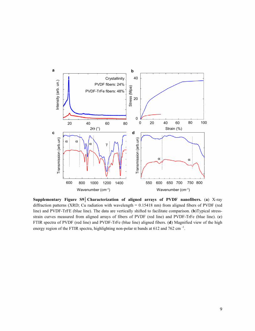
Supplementary Figure S9│Characterization of aligned arrays of PVDF nanofibers. (a) X-ray diffraction patterns (XRD; Cu radiation with wavelength = 0.15418 nm) from aligned fibers of PVDF (red line) and PVDF-TrFE (blue line). The data are vertically shifted to facilitate comparison. (b)Typical stress-strain curves measured from aligned arrays of fibers of PVDF (red line) and PVDF-TrFe (blue line). (c) FTIR spectra of PVDF (red line) and PVDF-TrFe (blue line) aligned fibers. (d) Magnified view of the high

energy region of the FTIR spectra, highlighting non-polar α bands at 612 and 762 cm -1.

γαα

α

α α

550800 1000 1200 1400

Wavenumber (cm-1)

Tra

nsm

issi

on (

arb.

un)

600 650 700 750 800600

Wavenumber (cm-1)

Tra

nsm

issi

on (

arb.

un)

0 20 40 60 80 100

Strain (%)S

tres

s (M

pa)

0

20

40

a b

dc

Inte

nsity

(arb

. un.

)

20 40 60 802Θ (°)

Crystallinity

PVDF fibers: 24%

PVDF-TrFe fibers: 48%

10

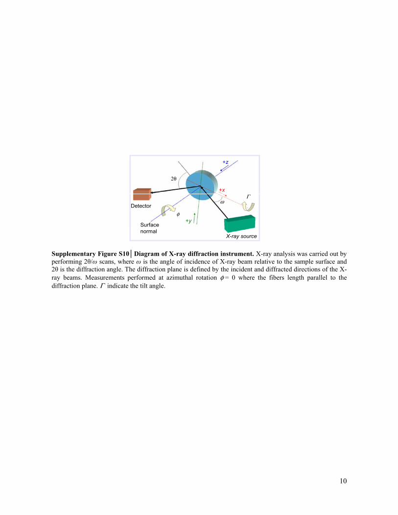
Supplementary Figure S10│Diagram of X-ray diffraction instrument. X-ray analysis was carried out by performing 2θ/ω scans, where ω is the angle of incidence of X-ray beam relative to the sample surface and 2θ is the diffraction angle. The diffraction plane is defined by the incident and diffracted directions of the X-ray beams. Measurements performed at azimuthal rotation φ = 0 where the fibers length parallel to the diffraction plane. Γ indicate the tilt angle.

Detector

Surfacenormal

φ+y

+x

+z

X-ray source

2θ

ωΓ

11

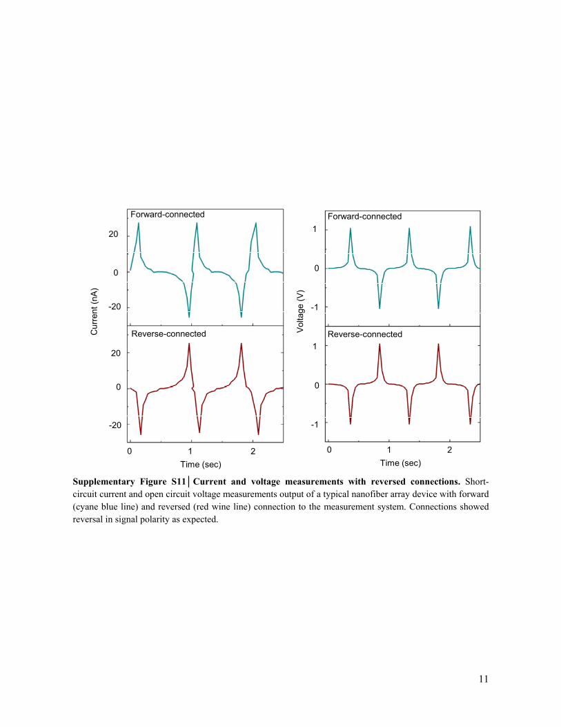
Supplementary Figure S11│Current and voltage measurements with reversed connections. Short-circuit current and open circuit voltage measurements output of a typical nanofiber array device with forward (cyane blue line) and reversed (red wine line) connection to the measurement system. Connections showed reversal in signal polarity as expected.

Time (sec)

Cur

rent

(nA

)

0 1 2

0

-20

20

-20

0

20

Vol

tage

(V

)

0

1

-1

0

1

-1

Time (sec)

0 1 2

Forward-connected Forward-connected

Reverse-connected Reverse-connected

12

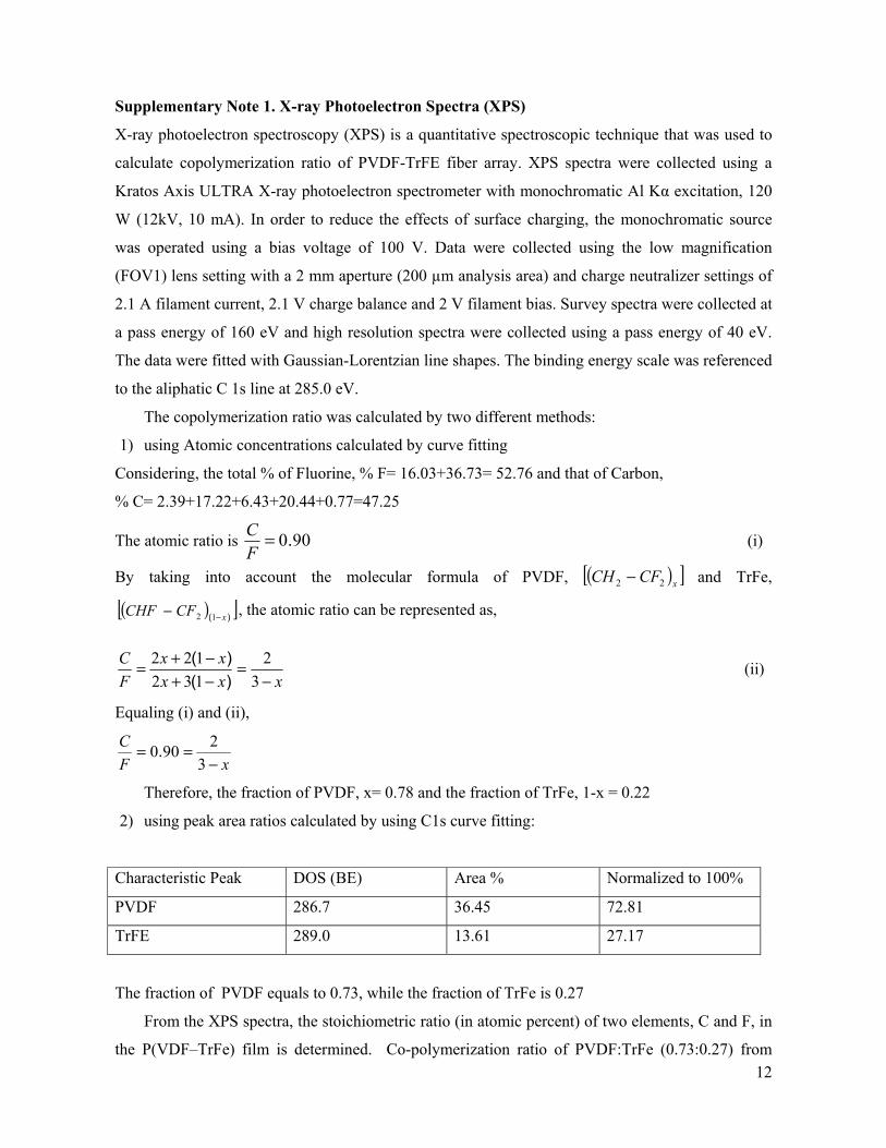
Supplementary Note 1. X-ray Photoelectron Spectra (XPS)

X-ray photoelectron spectroscopy (XPS) is a quantitative spectroscopic technique that was used to

calculate copolymerization ratio of PVDF-TrFE fiber array. XPS spectra were collected using a

Kratos Axis ULTRA X-ray photoelectron spectrometer with monochromatic Al Kα excitation, 120

W (12kV, 10 mA). In order to reduce the effects of surface charging, the monochromatic source

was operated using a bias voltage of 100 V. Data were collected using the low magnification

(FOV1) lens setting with a 2 mm aperture (200 µm analysis area) and charge neutralizer settings of

2.1 A filament current, 2.1 V charge balance and 2 V filament bias. Survey spectra were collected at

a pass energy of 160 eV and high resolution spectra were collected using a pass energy of 40 eV.

The data were fitted with Gaussian-Lorentzian line shapes. The binding energy scale was referenced

to the aliphatic C 1s line at 285.0 eV.

The copolymerization ratio was calculated by two different methods:

1) using Atomic concentrations calculated by curve fitting

Considering, the total % of Fluorine, % F= 16.03+36.73= 52.76 and that of Carbon,

% C= 2.39+17.22+6.43+20.44+0.77=47.25

The atomic ratio is 0 90.CF

= (i)

By taking into account the molecular formula of PVDF, ( )[ ]xCFCH 22 − and TrFe,

( )[ ])( xCFCHF −− 12 , the atomic ratio can be represented as,

xxx

xx

F

C

−=

−+−+=

3

2

132

122

)(

)( (ii)

Equaling (i) and (ii),

xF

C

−==

3

2900.

Therefore, the fraction of PVDF, x= 0.78 and the fraction of TrFe, 1-x = 0.22

2) using peak area ratios calculated by using C1s curve fitting:

Characteristic Peak DOS (BE) Area % Normalized to 100%

PVDF 286.7 36.45 72.81

TrFE 289.0 13.61 27.17

The fraction of PVDF equals to 0.73, while the fraction of TrFe is 0.27

From the XPS spectra, the stoichiometric ratio (in atomic percent) of two elements, C and F, in

the P(VDF–TrFe) film is determined. Co-polymerization ratio of PVDF:TrFe (0.73:0.27) from

13

XPS results shows excellent agreement with actual co-polymer ratio of commercial PVDF:TrFE

(0.75:0.25).

14

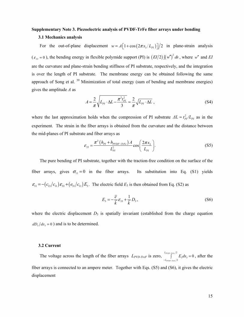
Supplementary Note 2. Piezoelectric analysis of PVDF-TrFe fiber arrays under compression

The constitutive model of piezoelectric materials gives the relations among the stress ijσ , strain ijε ,

electric field Ei and electric displacement Di as

( )

11 12 1311 11 31

12 11 1322 22 31

13 13 3333 33 33

4423 23 15

4431 31 15

11 1212 12

0 0 0 0 0

0 0 0 0 0

0 0 0 0 0

0 0 0 0 0 2 0 0

0 0 0 0 0 2 0 0

0 0 0 0 0 2 2 0 0 0

c c c e

c c c e

c c c e

c e

c e

c c

σ εσ εσ εσ εσ εσ ε

= −

−

1

2

3

E

E

E

, (S1)

11

221 15 11 1

332 15 22 2

233 31 31 33 33 3

31

12

0 0 0 0 0 0 0

0 0 0 0 0 0 02

0 0 0 0 02

2

D e k E

D e k E

D e e e k E

εεεεεε

= +

. (S2)

Consider a uniaxial compression applied along the x1 direction (normal to fibers, Fig. 3a)

instantaneously at time t=0, i.e., i.e., ( )11 pH tσ = − , where H is the Heavyside step function

( ) 0 0

1 0

for tH t

for t

<= ≥

. For 22 33 0ε ε= ≈ because the P(VDF-TrFE) fiber arrays (elastic modulus ~

200 MPa) are bonded to the much thicker and stiffer plastic substrate (elastic modulus 2.5 GPa),

Eqs. (S1) and (S2) give ( ) 11 11 31 3pH t c e Eε− = − and 3 31 11 33 3D e k Eε= + , respectively, where D3 is

the electric displacement along the poling direction, and the electric field 3E is related to the

voltage V and effective contact length Leff by 3 effE V L= . Elimination of 11ε from these two

equations yields the electric displacement ( ) ( )3 effD dpH t kV L= − + , where 31 11d e c= and

233 31 11k k e c= + . The voltage V and current 3PVDF TrFe PVDF TrFeI h w D− −= − are also related by the

resistance R of the voltmeter, V=IR. These yield the coupling equation of the voltage

( )eff eff

PVDF TrFe PVDF TrFe

L dLdVV t

dt kh w R kδ

− −

+ = , (S3)

where ( )tδ is the delta function. For the initial condition ( )0 0V t −= = , the solution of Eq. (S3) is

( ) ( )expeff eff PVDF TrFe PVDF TrFeV dL k p L t kRh w− − = − . The maximum value is given in Eq. (1) in the

main text.

15

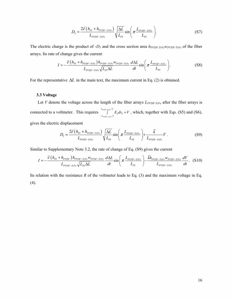
Supplementary Note 3. Piezoelectric analysis of PVDF-TrFe fiber arrays under bending

3.1 Mechanics analysis

For the out-of-plane displacement ( )31 cos 2 2PIw A x Lπ= + in plane-strain analysis

( 22 0ε = ), the bending energy in flexible polymide support (PI) is ( ) ( )22EI w ds′′ , where w′′ and EI

are the curvature and plane-strain bending stiffness of PI substrate, respectively, and the integration

is over the length of PI substrate. The membrane energy can be obtained following the same

approach of Song et al. 39 Minimization of total energy (sum of bending and membrane energies)

gives the amplitude A as

2 22 2

3PI

PI PI

tA L L L L

ππ π

= ⋅Δ − ≈ ⋅Δ , (S4)

where the last approximation holds when the compression of PI substrate PIPI /LtΔL 2≈ as in the

experiment. The strain in the fiber arrays is obtained from the curvature and the distance between

the mid-planes of PI substrate and fiber arrays as

( )23

33 2

2cosPI PVDF TrFe

PI PI

h h A x

L L

π πε −+ =

. (S5)

The pure bending of PI substrate, together with the traction-free condition on the surface of the

fiber arrays, gives 11 0σ = in the fiber arrays. Its substitution into Eq. (S1) yields

( ) ( )11 13 11 33 31 11 3c c e c Eε ε= − + . The electric field E3 is then obtained from Eq. (S2) as

3 33 3

1eE D

k kε= − + , (S6)

where the electric displacement D3 is spatially invariant (established from the charge equation

3 3 0dD dx = ) and is to be determined.

3.2 Current

The voltage across the length of the fiber arrays LPVD-TreF is zero, 2

3 32

0PVDF TrFe

PVDF TrFe

L

L

E dx−

−−= , after the

fiber arrays is connected to an ampere meter. Together with Eqs. (S5) and (S6), it gives the electric

displacement

16

( )

3

2sinPI PVDF TrFe PVDF TrFe

PVDF TrFe PI PI

e h h LLD

L L Lπ− −

−

+ Δ=

. (S7)

The electric charge is the product of -D3 and the cross section area hPVDF-TrFewPVDF-TrFe of the fiber

arrays. Its rate of change gives the current

( )

sinPI PVDF TrFe PVDF TrFe PVDF TrFe PVDF TrFe

PIPVDF TrFe PI

e h h h w Ld LI

dt LL L Lπ− − − −

−

+ Δ= − Δ . (S8)

For the representative LΔ in the main text, the maximum current in Eq. (2) is obtained.

3.3 Voltage

Let V denote the voltage across the length of the fiber arrays LPVDF-TrFe after the fiber arrays is

connected to a voltmeter. This requires 2

3 32

PVDF TrFe

PVDF TrFe

L

L

E dx V−

−−= , which, together with Eqs. (S5) and (S6),

gives the electric displacement

( )

3

2sinPI PVDF TrFe PVDF TrFe

PVDF TrFe PI PI PVDF TrFe

e h h LL kD V

L L L Lπ− −

− −

+ Δ= +

. (S9)

Similar to Supplementary Note 3.2, the rate of change of Eq. (S9) gives the current

( )

sinPI PVDF PVDF TrFe PVDF TrFe PVDF TrFe PVDF TrFe PVDF TrFe

PI PVDF TrFePVDF TrFe PI

e h h h w L kh wd L dVI

dt L L dtL L Lπ− − − − −

−−

+ Δ= − − Δ . (S10)

Its relation with the resistance R of the voltmeter leads to Eq. (3) and the maximum voltage in Eq.

(4).

17

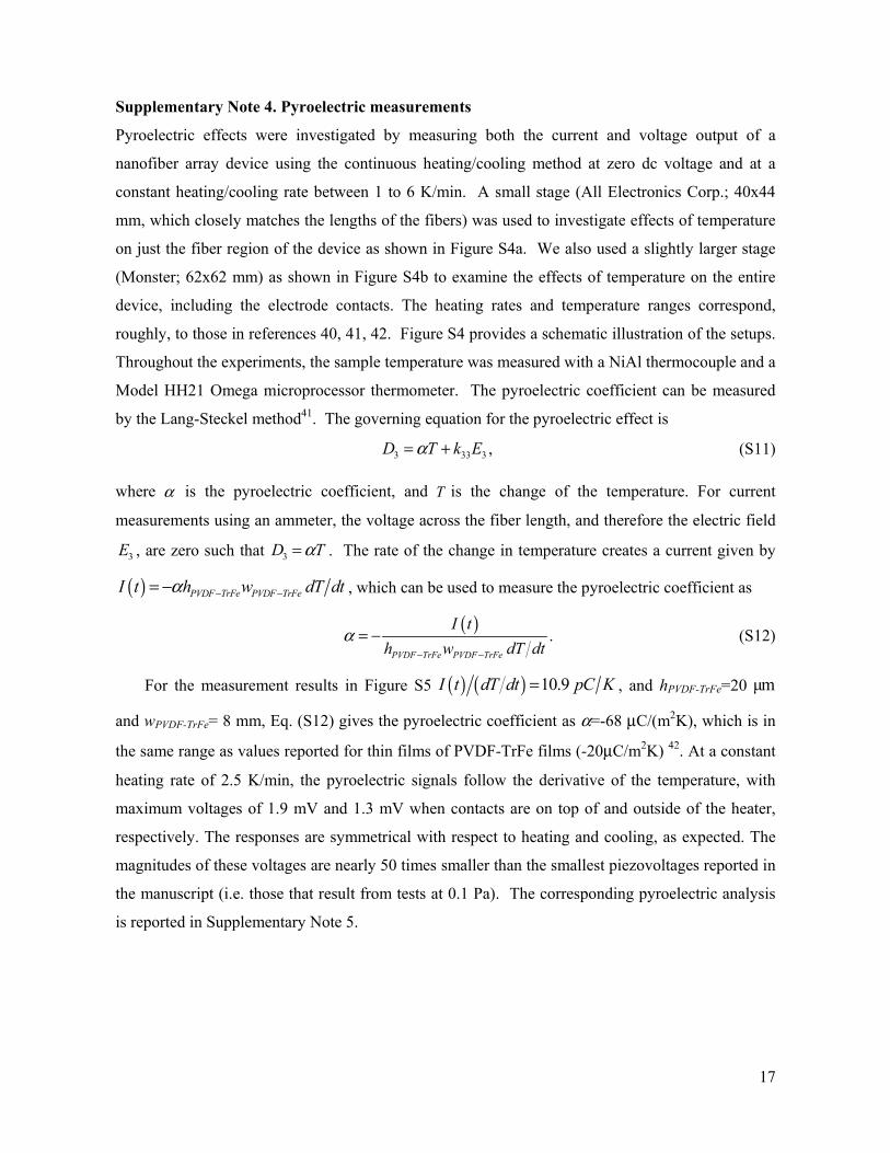
Supplementary Note 4. Pyroelectric measurements

Pyroelectric effects were investigated by measuring both the current and voltage output of a

nanofiber array device using the continuous heating/cooling method at zero dc voltage and at a

constant heating/cooling rate between 1 to 6 K/min. A small stage (All Electronics Corp.; 40x44

mm, which closely matches the lengths of the fibers) was used to investigate effects of temperature

on just the fiber region of the device as shown in Figure S4a. We also used a slightly larger stage

(Monster; 62x62 mm) as shown in Figure S4b to examine the effects of temperature on the entire

device, including the electrode contacts. The heating rates and temperature ranges correspond,

roughly, to those in references 40, 41, 42. Figure S4 provides a schematic illustration of the setups.

Throughout the experiments, the sample temperature was measured with a NiAl thermocouple and a

Model HH21 Omega microprocessor thermometer. The pyroelectric coefficient can be measured

by the Lang-Steckel method41. The governing equation for the pyroelectric effect is

3 33 3D T k Eα= + , (S11)

where α is the pyroelectric coefficient, and T is the change of the temperature. For current

measurements using an ammeter, the voltage across the fiber length, and therefore the electric field

3E , are zero such that 3D Tα= . The rate of the change in temperature creates a current given by

( ) PVDF TrFe PVDF TrFeI t h w dT dtα − −= − , which can be used to measure the pyroelectric coefficient as

( )

PVDF TrFe PVDF TrFe

I t

h w dT dtα

− −

= − . (S12)

For the measurement results in Figure S5 ( ) ( ) 10.9I t dT dt pC K= , and hPVDF-TrFe=20 μm

and wPVDF-TrFe= 8 mm, Eq. (S12) gives the pyroelectric coefficient as α=-68 μC/(m2K), which is in

the same range as values reported for thin films of PVDF-TrFe films (-20μC/m2K) 42. At a constant

heating rate of 2.5 K/min, the pyroelectric signals follow the derivative of the temperature, with

maximum voltages of 1.9 mV and 1.3 mV when contacts are on top of and outside of the heater,

respectively. The responses are symmetrical with respect to heating and cooling, as expected. The

magnitudes of these voltages are nearly 50 times smaller than the smallest piezovoltages reported in

the manuscript (i.e. those that result from tests at 0.1 Pa). The corresponding pyroelectric analysis

is reported in Supplementary Note 5.

18

Supplementary Note 5. Pyroelectric analysis

For voltage measurement of the fiber arrays via a voltmeter, Eq. (S11) still holds. The electric field

3E and electric displacement D3 are related to the voltage V and current I by 3 PVDF TrFeE V L −= and

3PVDF TrFe PVDF TrFeI h w D− −= − , respectively, where PVDF TrFeL − is the length of fiber arrays and

PVDF TrFe PVDF TrFeh w− − is the cross section area. The voltage V and current I are also related by the

resistance R of the voltmeter, V=IR. These give the equation for V as

33 33

PVDF TrFe PVDF TrFe

PVDF TrFe PVDF TrFe

L LdV dTV

dt k Rh w k dt

α− −

− −

+ = − . (S16)

For the initial condition ( )0 0V t = = , the above equation has the solution

( )

33

33 0

PVDF TrFe

PVDF TrFe PVDF TrFe

Lt tk Rh wPVDF TrFeL dT

V e dk d

τα ττ

−

− −−

−= − . (S17)

For LPVDF-TrFe=40 mm, thickness hPVDF=20 μm , width wPVDF-TrFe=8 mm, and the measured

pyroelectric coefficient 68α = − ( )2μC m K and resistance of the voltmeter R=4 MΩ in

experiments, the maximum voltage is 1.81 μV for the measured temperature T(t) in Fig. S6 and the

dielectric constant k33=5.31*10-11 F/m 38. In fact, for the normalized time ( )33 1PVDF TrFeL t Sk R− ,

Eq. (S17) can be simplified to Eq. (5) in the main text, which also gives the maximum voltage 1.81

V, and agrees well with maximum voltage of 1.9 V when the PVDF-TrFe fiber arrays are in contact

with the top of the heater.

It should be pointed out that different voltmeters were used for pyroelectric and piezoelectric

measurements, with resistance of the voltmeter R=4 MΩ and 70 MΩ, respectively due to different

sensing range of voltmeters. Even for R=70 MΩ and heating rate 6.5 K/min, the pyroelectric

voltage is still smaller than the piezoelectric voltage even at the lower end of the range of pressure

sensitivity (0.1 Pa, in the type of tests reported here).

19

Supplementary Note 6. Comparison between PVDF-TrFe and PVDF fibers

For purposes of comparison, PVDF fibers were formed with the same experimental conditions used

for PVDF-TrFe. In particular, PVDF (Sigma Aldrich) was dissolved in a 3:2 volume ratio of

dimethylformamide/acetone at a polymer/solvent concentration of 21% w/w. A potential of 30 kV

was applied between a nozzle tip with inner diameter of 200 μm, fed by a syringe pump at a flow-

rate of 1 mL/hr, and a collector at a distance of 6 cm. The collector disk rotated at angular speed of

4000 rpm, corresponding to linear speeds > 16 m/s at the collector surface. The fibers were

collected on aluminium strips with widths of 0.8 cm and lengths of 25 cm. The morphological,

crystallographic and mechanical properties of PVDF fibers were measured and compared with those

of PVDF-TrFe. The most immediate, striking difference from PVDF-TrFe was that the PVDF fibers

were not sufficiently robust to exist as stable, free-standing films. In nearly all cases the process of

detaching the PVDF fibers from the aluminium foil mechanically destroyed the samples by fracture

and tearing. Furthermore, we found that PVDF fibers are poorly aligned (Figure S8a). 2D FFT

analysis indicates that the full width at half maximum of the radial intensity distribution of the

elliptical profile is 51°, which is more than three times larger than that of the PVDF-TrFe arrays

(Figure S8b). Although the average fiber diameters (250 nm) and the corresponding distribution of

diameters are comparable (Figure S8c), the surfaces of the PVDF fibers are rough, with protrusions

that have characteristic dimensions of ~100 nm (Inset of Figure S9a). X-ray diffraction (XRD)

patterns indicate that PVDF fibers exhibit 24% crystallinity, which is two times lower than that of

PVDF-TrFe fibers (Figure S9a) and the non-polar α (612,762, 976 cm-1) and γ (1234 cm-1) phases

are here clearly distinguishable by FTIR (Figure S9c and d). The mechanical properties were

investigated using dynamic mechanical analysis (DMA Q800, TA Instruments, New Castle, DE), in

tensile mode at constant temperature (25°C). At least three different fibrous specimens for each

polymer were tested. Specimen dimensions were approximately 8.0×12.0 mm (width×length) with

thicknesses between 20 and 40 μm. The stress-strain curves were recorded with a ramp/rate of 0.5

N/min (up to 18 N). Typical stress-strain curves of PVDF and PVDF-TrFe fibers are reported in

Figure S9b. The measured Young Modulus is 168 ±8 MPa for PVDF-TrFe and 86 ±11 MPa for

PDVF fibers respectively. The maximum elongation of PVDF-TrFE fibers is ~100%

(corresponding to a tensile strength of about 40 MPa) while that of PVDF fibers is ~32%

(corresponding to a tensile strength of about 5 MPa). These results clearly indicate that PVDF-TrFe

fibers exhibit superior mechanical properties compared to PVDF fibers. Such differences are

critically important to use in the classes of devices described in our manuscript. In addition, the

formation of inter-fibers joints or adhesion points further increase both the tensile strength and the

elongation path44.

20

Supplementary Methods . PVDF-TrFe fibers made with low-boiling solvents

PVDF-TrFe was dissolved in three different low-boiling point (Tb) solvents: Acetone (ACE, Tb:

57°C), Tetrahydrofuran (THF, Tb: 66°C) and methylethylketone (MEK, Tb: 80°C) at different

polymer/solvent concentrations in the range 12-21% (w/w). At the highest concentration, needle

clogging occurs almost instantaneously with ACE and THF (Figure S7 a and b respectively), and

after tens of seconds with MEK (Figure S7c). In this last case, collected fibers take the form of

isolated strands (about 7 x102 roughly parallel fibers per mm) with an average diameter ~570 nm.

Such fibers have non-uniform morphologies, with both flat and porous surfaces, and in short,

discontinuous segments due to the presence of necks and beads (Figure S7d).

At lower concentrations, the maximum electrospinning time could be extended to ~15 minutes

with ACE (corresponding to 300 μL of solution at the lowest concentration of 12% w/w) before

needle clogging stopped irreversibly the electrospinning process. Fibers in this case appear in the

form of isolated strands (2 x 103 fibers per mm) with an average diameter of ~340 nm. As with

MEK, fiber continuity is interrupted due to the formation of numerous beads (width of 2-8 μm and

length of 5-20 μm) and the surface morphology of the fibers is inhomogeneous. In general, such

discontinuities are observed at any solution concentration (Figure S7e).

Using THF, electrospinning was not interrupted by needle clogging, but the produced fibers

are, nevertheless, discontinuous with beads and a large variety of surface morphologies. Fibers

exhibit an average diameter of ~570 nm, and a density below 1x103 fibers per mm for solutions at

12% polymer/solvent (Figure S7f). Finally in case of MEK beads and surface discontinuity can be

strongly reduced but the resulting fibers are still in the form of isolated strands (1x 102 fibers per

mm) with an average diameter of 590 nm even after 1 hour of continuous spinning (Figure S7g).

21

Supplementary References

44. Rizvi, M. S., Kumar, P., Katti, D. S. & Pal A. Mathematical model of mechanical behavior of

micro/nanofibrous materials designed for extracellular matrix substitutes. Acta Biomaterialia 8,

4111–4122, (2012).