Graphical Models

Michael I. Jordan

Computer Science Division and Department of Statistics

University of California, Berkeley 94720

Abstract

Statistical applications in fields such as bioinformatics, information retrieval, speech processing, im-

age processing and communications often involve large-scale models in which thousands or millions

of random variables are linked in complex ways. Graphical models provide a general methodology

for approaching these problems, and indeed many of the models developed by researchers in these

applied fields are instances of the general graphical model formalism. We review some of the basic

ideas underlying graphical models, including the algorithmic ideas that allow graphical models to

be deployed in large-scale data analysis problems. We also present examples of graphical models

in bioinformatics, error-control coding and language processing.

Keywords: Probabilistic graphical models; junction tree algorithm; sum-product algorithm; Markov

chain Monte Carlo; variational inference; bioinformatics; error-control coding.

1. Introduction

The fields of Statistics and Computer Science have generally followed separate paths for the past

several decades, which each field providing useful services to the other, but with the core concerns

of the two fields rarely appearing to intersect. In recent years, however, it has become increasingly

evident that the long-term goals of the two fields are closely aligned. Statisticians are increasingly

concerned with the computational aspects, both theoretical and practical, of models and inference

procedures. Computer scientists are increasingly concerned with systems that interact with the

external world and interpret uncertain data in terms of underlying probabilistic models. One area

in which these trends are most evident is that of probabilistic graphical models.

A graphical model is a family of probability distributions defined in terms of a directed or

undirected graph. The nodes in the graph are identified with random variables, and joint probability

1

distributions are defined by taking products over functions defined on connected subsets of nodes.

By exploiting the graph-theoretic representation, the formalism provides general algorithms for

computing marginal and conditional probabilities of interest. Moreover, the formalism provides

control over the computational complexity associated with these operations.

The graphical model formalism is agnostic to the distinction between frequentist and Bayesian

statistics. However, by providing general machinery for manipulating joint probability distribu-

tions, and in particular by making hierarchical latent variable models easy to represent and manip-

ulate, the formalism has proved to be particularly popular within the Bayesian paradigm. Viewing

Bayesian statistics as the systematic application of probability theory to statistics, and viewing

graphical models as a systematic application of graph-theoretic algorithms to probability theory,

it should not be surprising that many authors have viewed graphical models as a general Bayesian

“inference engine”(Cowell et al., 1999).

What is perhaps most distinctive about the graphical model approach is its naturalness in

formulating probabilistic models of complex phenomena in applied fields, while maintaining control

over the computational cost associated with these models. Accordingly, in this article our principal

focus is on the presentation of graphical models that have proved useful in applied domains, and on

ways in which the formalism encourages the exploration of extensions of classical methods. Before

turning to these examples, however, we begin with an overview of basic concepts.

2. Representation

The two most common forms of graphical model are directed graphical models and undirected

graphical models, based on directed acylic graphs and undirected graphs, respectively.

Let us begin with the directed case. Let G(V, E) be a directed acyclic graph, where V are the

nodes and E are the edges of the graph. Let {Xv : v ∈ V} be a collection of random variables indexed

by the nodes of the graph. To each node v ∈ V , let πv denote the subset of indices of its parents.

We allow sets of indices to appear wherever a single index appears, thus Xπv denotes the vector of

random variables indexed by the parents of v. Given a collection of kernels, {k(xv |xπv) : v ∈ V},

2

1Z 2Z 3Z NZ

θ

N

θ

nZ

(a) (b)

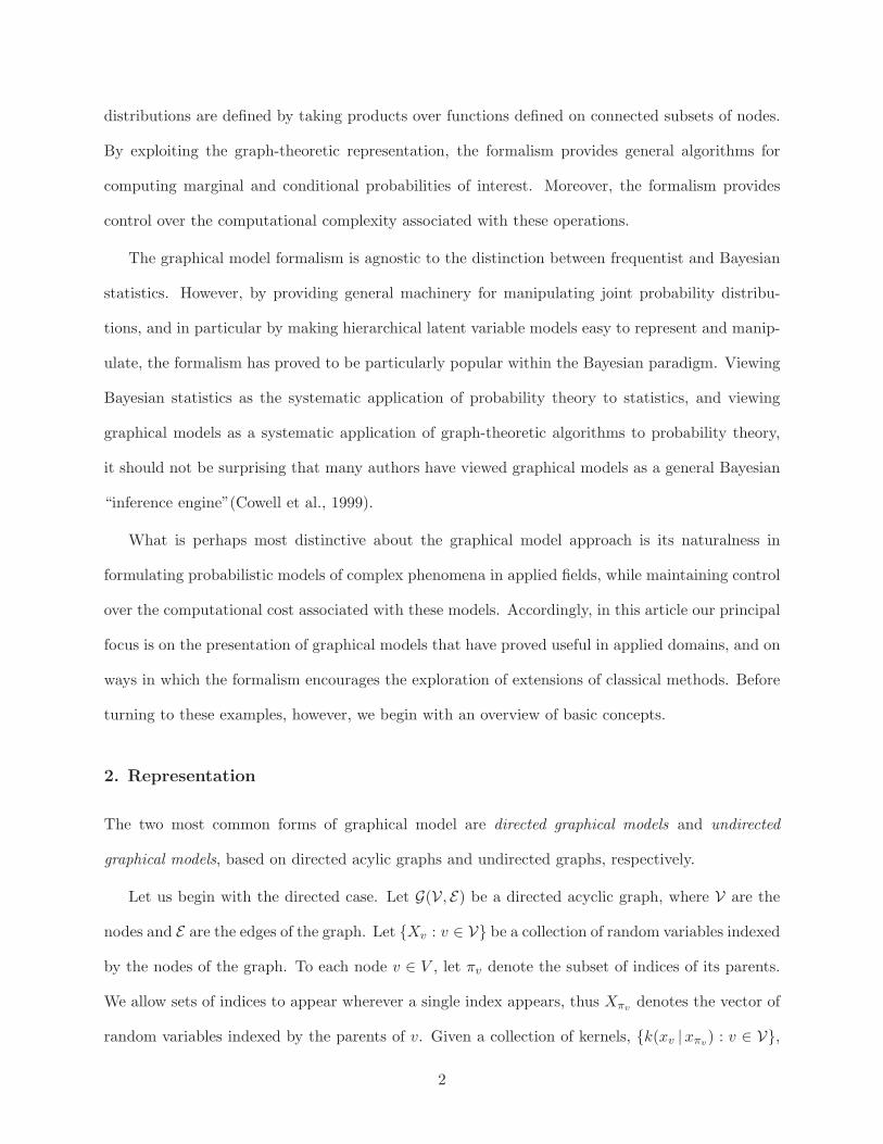
Figure 1: The diagram in (a) is a shorthand for the graphical model in (b). This model asserts

that the variables Zn are conditionally independent and identically distributed given θ,

and can be viewed as a graphical model representation of the De Finetti theorem. Note

that shading, here and elsewhere in the paper, denotes conditioning.

that sum (in the discrete case) or integrate (in the continuous case) to one (with respect to xv),

we define a joint probability distribution (a probability mass function or probability density as

appropriate) as follows:

p(xV) =∏v∈V

k(xv |xπv). (1)

It is easy to verify that this joint probability distribution has {k(xv |xπv)} as its conditionals; thus,

henceforth, we write k(xv |xπv) = p(xv |xπv).

Note that we have made no distinction between data and parameters, and indeed it is natural

to include parameters among the nodes in the graph.

A plate is a useful device for capturing replication in graphical models, including the facto-

rial and nested structures that occur in experimental designs. A simple example of a plate is

shown in Figure 1; this figure can be viewed as a graphical model representation of the de Finetti

exchangeability theorem.

Directed graphical models are familiar as representations of hierarchical Bayesian models. An

example is given in Figure 2.

3

X

Z

Y U

K

C

N

θ

λ

β

W

i

i

i

i i

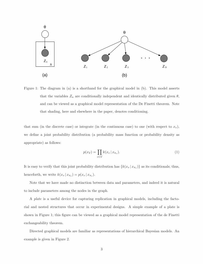
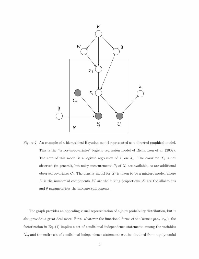
Figure 2: An example of a hierarchical Bayesian model represented as a directed graphical model.

This is the “errors-in-covariates” logistic regression model of Richardson et al. (2002).

The core of this model is a logistic regression of Yi on Xi. The covariate Xi is not

observed (in general), but noisy measurements Ui of Xi are available, as are additional

observed covariates Ci. The density model for Xi is taken to be a mixture model, where

K is the number of components, W are the mixing proportions, Zi are the allocations

and θ parameterizes the mixture components.

The graph provides an appealing visual representation of a joint probability distribution, but it

also provides a great deal more. First, whatever the functional forms of the kernels p(xv |xπv), the

factorization in Eq. (1) implies a set of conditional independence statements among the variables

Xv, and the entire set of conditional independence statements can be obtained from a polynomial

4

1X

2X

3X

X 4

X 5

X6

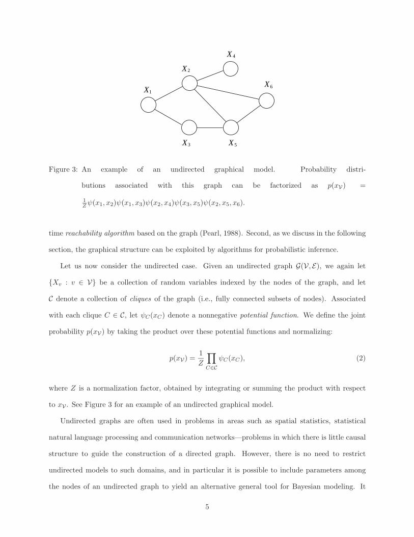
Figure 3: An example of an undirected graphical model. Probability distri-

butions associated with this graph can be factorized as p(xV) =

1Zψ(x1, x2)ψ(x1, x3)ψ(x2, x4)ψ(x3, x5)ψ(x2, x5, x6).

time reachability algorithm based on the graph (Pearl, 1988). Second, as we discuss in the following

section, the graphical structure can be exploited by algorithms for probabilistic inference.

Let us now consider the undirected case. Given an undirected graph G(V, E), we again let

{Xv : v ∈ V} be a collection of random variables indexed by the nodes of the graph, and let

C denote a collection of cliques of the graph (i.e., fully connected subsets of nodes). Associated

with each clique C ∈ C, let ψC(xC) denote a nonnegative potential function. We define the joint

probability p(xV) by taking the product over these potential functions and normalizing:

p(xV) =1Z

∏C∈C

ψC(xC), (2)

where Z is a normalization factor, obtained by integrating or summing the product with respect

to xV . See Figure 3 for an example of an undirected graphical model.

Undirected graphs are often used in problems in areas such as spatial statistics, statistical

natural language processing and communication networks—problems in which there is little causal

structure to guide the construction of a directed graph. However, there is no need to restrict

undirected models to such domains, and in particular it is possible to include parameters among

the nodes of an undirected graph to yield an alternative general tool for Bayesian modeling. It

5

is also possible to work with hybrids that include both directed and undirected edges (Lauritzen,

1996).

In general, directed graphs and undirected graphs make different assertions of conditional in-

dependence. Thus, there are families of probability distributions that are captured by a directed

graph and are not captured by any undirected graph, and vice versa (Pearl, 1988).

The representations shown in Eq. (1) and Eq. (2) can be overly coarse for some purposes. In

particular, in the undirected formalism the cliques C may be quite large, and it is often useful to

consider potential functions that are themselves factorized, in ways that need not be equated with

conditional independencies. Thus, in general, we consider a set of “factors,” {fi(xCi) : i ∈ I}, for

some index set I, where Ci is the subset of nodes associated with the ith factor. Note in particular

that the same subset can be repeated multiple times (i.e., we allow Ci = Cj for i �= j). We define

a joint probability by taking the product across these factors:

p(xV) =1Z

∏i∈I

fi(xCi). (3)

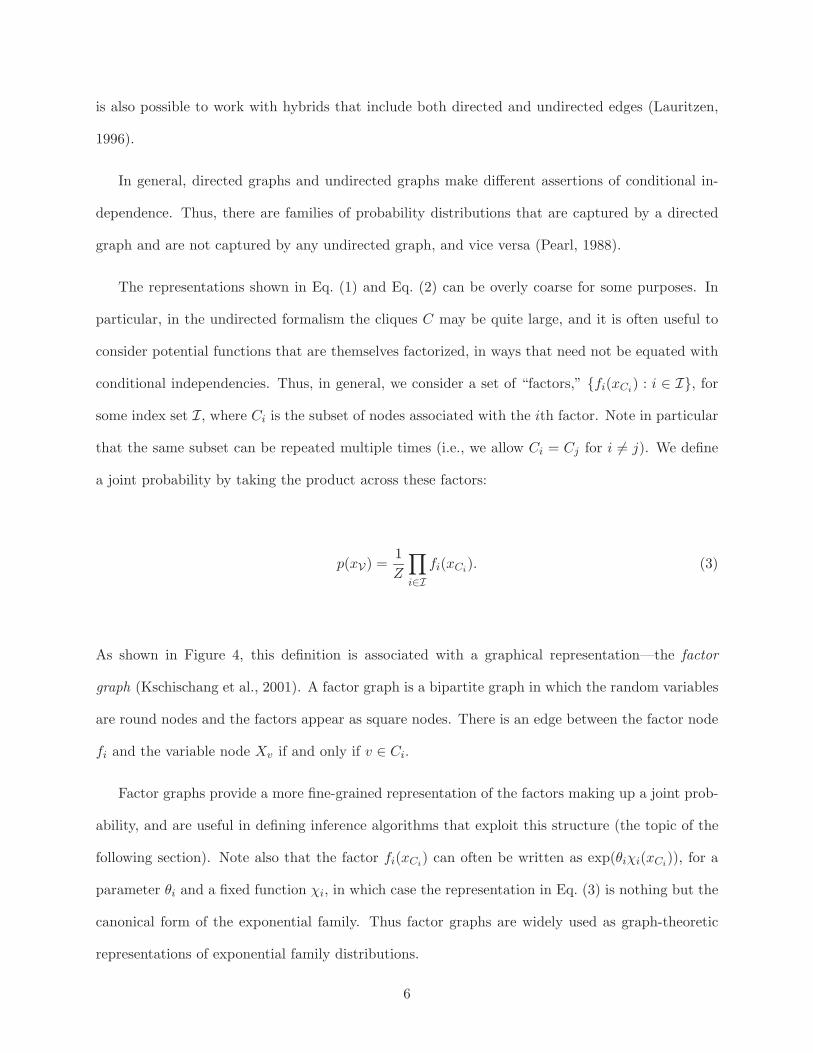
As shown in Figure 4, this definition is associated with a graphical representation—the factor

graph (Kschischang et al., 2001). A factor graph is a bipartite graph in which the random variables

are round nodes and the factors appear as square nodes. There is an edge between the factor node

fi and the variable node Xv if and only if v ∈ Ci.

Factor graphs provide a more fine-grained representation of the factors making up a joint prob-

ability, and are useful in defining inference algorithms that exploit this structure (the topic of the

following section). Note also that the factor fi(xCi) can often be written as exp(θiχi(xCi)), for a

parameter θi and a fixed function χi, in which case the representation in Eq. (3) is nothing but the

canonical form of the exponential family. Thus factor graphs are widely used as graph-theoretic

representations of exponential family distributions.

6

1X 2X 3X X 4 X 5

af bf cf df

Figure 4: An example of a factor graph. Probability distributions associated with this graph can

be factorized as p(xV) = 1Z fa(x1, x3)fb(x3, x4)fc(x2, x4, x5)fd(x1, x3).

3. Algorithms for probabilistic inference

The general problem of probabilistic inference is that of computing conditional probabilities p(xF |xE),

where V = E ∪ F ∪H for given subsets E, F and H. In this section we are concerned with algo-

rithms for performing such computations, and the role that graphical structure can play in making

such computations efficient.

In discussing inference algorithms, it proves useful to treat directed graphs and undirected

graphs on an equal footing. This is done by converting the former to the latter. Note in particular

that Eq. (1) could be treated as a special case of Eq. (2) if it were the case that each factor p(xi |xπi)

were a function on a clique. In general, however, the parents πi of a given node i are not connected,

and so the set πi ∪ {i} is not a clique. We can force this set to be a clique by adding (undirected)

edges between all of the parents πi, essentially constructing a new graph that is a graphical cover

of the original graph. If we also convert the directed edges (from parents to children) to undirected

edges, the result is an undirected graphical cover—the so-called moral graph—in which all of the

arguments of the function p(xi |xπi) are contained in a clique. That is, in the moral graph, the

factorization in Eq. (1) is a special case of Eq. (2). Thus we can proceed by working exclusively

within the undirected formalism.

7

It is also useful to note that from a computational point of view the conditioning plays little

essential role in the problem. Indeed, to condition on the event {XE = xE}, it suffices to redefine the

original clique potentials. Thus, for i ∈ E , we multiply the potential ψC(xC) by the Kronecker delta

function δ(xi), for any C such that {i} ∈ C∩E. The result is an unnormalized representation of the

conditional probability that has the factorized form in Eq. (2). Thus, from a computational point

of view, it suffices to focus on the problem of marginalization of the general factorized expression in

Eq. (2). We are interested in controlling the growth in computational complexity of performing such

marginalization, as a function of the cardinality of V. In the following three sections, we describe

the three principal classes of methods that attempt to deal with this computational issue—exact

algorithms, sampling algorithms, and variational algorithms. Our presentation will be brief; for a

fuller presentation see Cowell et al. (1999) and Jordan (1999).

3.1 Exact algorithms

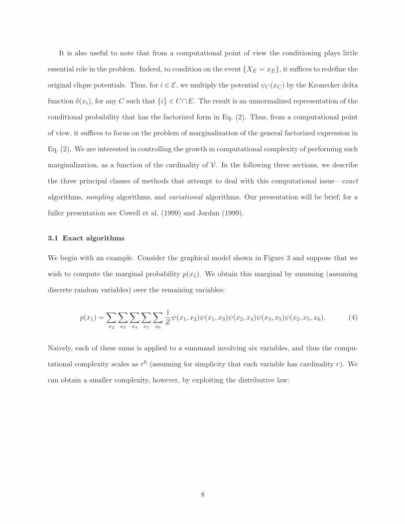
We begin with an example. Consider the graphical model shown in Figure 3 and suppose that we

wish to compute the marginal probability p(x1). We obtain this marginal by summing (assuming

discrete random variables) over the remaining variables:

p(x1) =∑x2

∑x3

∑x4

∑x5

∑x6

1Zψ(x1, x2)ψ(x1, x3)ψ(x2, x4)ψ(x3, x5)ψ(x2, x5, x6). (4)

Naively, each of these sums is applied to a summand involving six variables, and thus the compu-

tational complexity scales as r6 (assuming for simplicity that each variable has cardinality r). We

can obtain a smaller complexity, however, by exploiting the distributive law:

8

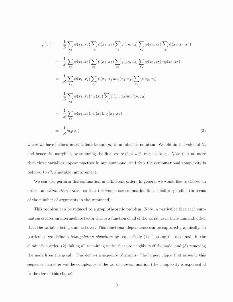
p(x1) =1Z

∑x2

ψ(x1, x2)∑x3

ψ(x1, x3)∑x4

ψ(x2, x4)∑x5

ψ(x3, x5)∑x6

ψ(x2, x5, x6)

=1Z

∑x2

ψ(x1, x2)∑x3

ψ(x1, x3)∑x4

ψ(x2, x4)∑x5

ψ(x3, x5)m6(x2, x5)

=1Z

∑x2

ψ(x1, x2)∑x3

ψ(x1, x3)m5(x2, x3)∑x4

ψ(x2, x4)

=1Z

∑x2

ψ(x1, x2)m4(x2)∑x3

ψ(x1, x3)m5(x2, x3)

=1Z

∑x2

ψ(x1, x2)m4(x2)m3(x1, x2)

=1Zm2(x1), (5)

where we have defined intermediate factors mi in an obvious notation. We obtain the value of Z,

and hence the marginal, by summing the final expression with respect to x1. Note that no more

than three variables appear together in any summand, and thus the computational complexity is

reduced to r3, a notable improvement.

We can also perform this summation in a different order. In general we would like to choose an

order—an elimination order—so that the worst-case summation is as small as possible (in terms

of the number of arguments in the summand).

This problem can be reduced to a graph-theoretic problem. Note in particular that each sum-

mation creates an intermediate factor that is a function of all of the variables in the summand, other

than the variable being summed over. This functional dependence can be captured graphically. In

particular, we define a triangulation algorithm by sequentially (1) choosing the next node in the

elimination order, (2) linking all remaining nodes that are neighbors of the node, and (3) removing

the node from the graph. This defines a sequence of graphs. The largest clique that arises in this

sequence characterizes the complexity of the worst-case summation (the complexity is exponential

in the size of this clique).

9

The minimum (over elimination orders) of the size of the maximal clique is known as the

treewidth of the graph.1 To minimize the computational complexity of inference, we wish to choose

an elimination ordering that achieves the treewidth. This is a graph-theoretic problem—it is

independent of the numerical values of the potentials.2

The problem of finding an elimination ordering that achieves the treewidth turns out to be

NP-hard (Arnborg et al., 1987). It is often possible in practice, however, to find good or even

optimal orderings for specific graphs, and a variety of inference algorithms in specific fields (e.g.,

the algorithms for inference on phylogenies and pedigrees in Section 4.1) have been based on specific

choices of elimination orderings in problems of interest. In general this class of algorithms is known

as probabilistic elimination, and it forms an important class of exact inference algorithms.

A limitation of the elimination approach to inference is that it yields only a single marginal prob-

ability. We often require more than one marginal probability, and we wish to avoid the inefficiency

of requiring multiple runs of an elimination algorithm.

To see how to compute general marginal probabilities, let us first restrict ourselves to the special

case in which the graph is a tree. In an undirected tree, the cliques are pairs of nodes and singleton

nodes, and thus the probability distribution is parameterized with potentials {ψ(xi, xj) : (i, j) ∈ E}

and {ψ(xi) : i ∈ V}. To compute a specific marginal, p(xf ), consider a rooted tree in which node f

is taken to be the root of the tree, and choose an elimination order in which all children of any node

are eliminated before the node itself is eliminated. Given this choice, the steps of the elimination

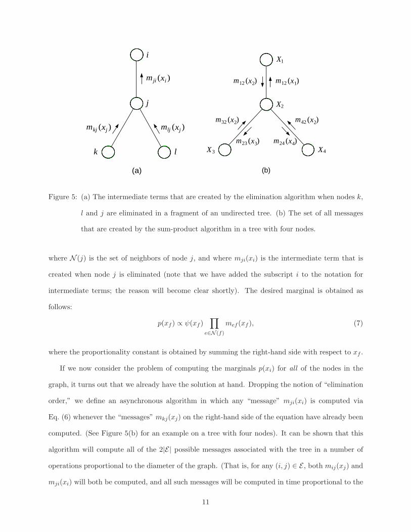
algorithm can be written in the following general way (see Figure 5(a)):

mji(xi) =∑xj

⎛⎝ψ(xj)ψ(xi, xj)

∏k∈N (j)\i

mkj(xj)

⎞⎠ , (6)

1. By convention the treewidth is actually one less than this maximal size.2. Moreover, it is also directly applicable to continuous variables. Replacing sums with integrals, and taking care with

regularity conditions, our characterization of computational complexity in graphical terms still applies. There is

of course the issue of computing individual integrals, which introduces additional computational considerations.

10

i

j

mji ( )xi

mkj ( )xj mlj ( )xj

k l

(a)

m32 ( )x2

m23 ( )x3

m12 ( )x2

m42 ( )x2

m24 ( )x4

m12 ( )x1

(b)

3X

2X

4X

1X

Figure 5: (a) The intermediate terms that are created by the elimination algorithm when nodes k,

l and j are eliminated in a fragment of an undirected tree. (b) The set of all messages

that are created by the sum-product algorithm in a tree with four nodes.

where N (j) is the set of neighbors of node j, and where mji(xi) is the intermediate term that is

created when node j is eliminated (note that we have added the subscript i to the notation for

intermediate terms; the reason will become clear shortly). The desired marginal is obtained as

follows:

p(xf ) ∝ ψ(xf )∏

e∈N (f)

mef (xf ), (7)

where the proportionality constant is obtained by summing the right-hand side with respect to xf .

If we now consider the problem of computing the marginals p(xi) for all of the nodes in the

graph, it turns out that we already have the solution at hand. Dropping the notion of “elimination

order,” we define an asynchronous algorithm in which any “message” mji(xi) is computed via

Eq. (6) whenever the “messages” mkj(xj) on the right-hand side of the equation have already been

computed. (See Figure 5(b) for an example on a tree with four nodes). It can be shown that this

algorithm will compute all of the 2|E| possible messages associated with the tree in a number of

operations proportional to the diameter of the graph. (That is, for any (i, j) ∈ E , both mij(xj) and

mji(xi) will both be computed, and all such messages will be computed in time proportional to the

11

length of the longest path in the graph). Once all messages have been computed, we compute the

marginal for any node via Eq. (7).

This algorithm is known as the sum-product algorithm. It is essentially a dynamic-programming-

like algorithm that achieves the effect of multiple elimination orders by computing the intermediate

terms that are needed for any given marginal only once, reusing these intermediate terms for other

marginals. In the case of discrete nodes with cardinality r, the algorithm has a computational

complexity of O(|E|r2).

The sum-product algorithm can be generalized in a number of ways. First, a variant of the

algorithm can be defined on factor graphs. In this case two kinds of messages are defined, in accor-

dance with the bipartite structure of factor graphs. Second, the algebraic operations that underly

the sum-product algorithm are justified by the fact that sums and products form a commutative

semiring, and the algorithm generalizes immediately to any other commutative semiring (Aji and

McEliece, 2000, Shenoy and Shafer, 1990). In particular, “maximization” and “product” form a

commutative semiring, and a “max-product” variant of the sum-product algorithm can be used for

computing modes of posterior distributions. Finally, as we now describe, a generalization of the

sum-product algorithm known as junction tree algorithm can be used for computing marginals in

general graphs.

The junction tree algorithm can be viewed as combining the ideas of the elimination algorithm

and the sum-product algorithm. The basic idea is to work with a tree-like data structure in which

the nodes are cliques rather than single nodes. (Such a graph is known as a hypergraph). A variant

of the sum-product algorithm is defined that defines messages that pass between cliques rather than

single nodes, and this algorithm is run on a tree of cliques. Which cliques do we use in forming

this tree? It turns out that it is not possible (in general) to use the cliques from the original

graph, but rather we must use the cliques from an augmented graph obtained by triangulating

the original graph. Conceptually we go through the operations associated with the elimination

algorithm, using a specific elimination ordering. Rather than actually performing these operations,

however, we perform only the graph-theoretic triangulation process. This defines a set of cliques,

12

which are formed into a tree. The sum-product algorithm running on this tree yields not only a

single marginal, but all marginals, where by “marginal” we now mean the marginal probability of

all variables in each clique. The computational complexity of the algorithm is determined by the

size of the largest clique, which is lower bounded by the treewidth of the graph.

In summary, exact inference algorithms such as the elimation algorithm, the sum-product algo-

rithm, and the junction tree algorithm compute marginal probabilities by systematically exploiting

the graphical structure; in essence exploiting the conditional independencies encoded in the pattern

of edges in the graph. In the best case, the treewidth of the graph is small, and an elimination

order that achieves the treewidth can be found easily. Many classical graphical models, including

hidden Markov models, trees, and the state-space models associated with Kalman filtering, are of

this kind. In general, however, the treewidth can be overly large, and in such cases exact algorithms

are not viable.

To see how to proceed in the case of more complex models, note that large treewidth heuristically

implies that the intermediate terms that are computed by the exact algorithms are sums of many

terms. This provides hope that there might be concentration phenomena that can be exploited by

approximate inference methods. These concentrations (if they exist) are necessarily dependent on

the specific numerical values of the potentials. In the next two sections, we overview some of the

algorithms that aim to exploit both the numerical and the graph-theoretic properties of graphical

models.

3.2 Sampling algorithms

Sampling algorithms such as importance sampling and Markov chain Monte Carlo (MCMC) provide

a general methodology for probabilistic inference (Liu, 2001, Robert and Casella, 2004). The

graphical model setting provides an opportunity for graph-theoretic structure to be exploited in

the design, analysis and implementation of sampling algorithms.

Note in particular that the class of MCMC algorithms known as Gibbs sampling requires the

computation of the probability of individual variables conditioned on all of the remaining variables.

13

The Markov properties of graphical models are useful here; conditioning on the so-called Markov

blanket of a given node renders the node independent of all other variables. In directed graphical

models, the Markov blanket is the set of parents, children and co-parents of a given node (“co-

parents” are nodes which have a child in common with the node). In the undirected case, the Markov

blanket is simply the set of neighbors of a given node. Using these definitions, Gibbs samplers can

be set up automatically from the graphical model specification, a fact that is exploited in the BUGS

software for Gibbs sampling in graphical models (Gilks et al., 1994). The Markov blanket is also

useful in the design of Metropolis-based algorithms—factors that do not appear in the Markov

blanket of a set of variables being considered in a proposed update can be neglected.

Finally, a variety of hybrid algorithms can be defined in which exact inference algorithms are

used locally within an overall sampling framework (Jensen et al., 1995, Murphy, 2002).

3.3 Variational algorithms

The basic idea of variational inference is to characterize a probability distribution as the solution

to an optimization problem, to perturb this optimization problem, and to solve the perturbed

problem. While these methods are applicable in principle to general probabilistic inference, thus

far their main domain of application has been to graphical models.

In their earliest application to general statistical inference, variational methods were formulated

in terms of the minimization of a Kullback-Leibler (KL) divergence, and the space over which the

optimization was performed was a set of “simplified” probability distributions, generally obtained

by removing edges from a graphical model (see Titterington, 2004, this volume). A more general

perspective has emerged, however, which relaxes the constraint that the optimization is performed

over a set of probability distributions, and no longer focuses on the KL divergence as the sole

optimization functional of interest. This approach can yield significantly tighter approximations.

We briefly overview the key ideas here; for a detailed presentation see Wainwright and Jordan

(2003).

14

We focus on finitely-parameterized probability distributions, which we express in exponential

family form. In particular, if we assume that each of the factors in Eq. (1), Eq. (2) or Eq. (3) can

be expressed in exponential family form, relative to a common measure ν, then the product of such

factors is also in exponential family form, and we write:

p(xV | θ) = exp{〈θ, φ(xV)〉 − A(θ)

}, (8)

where φ(xV) is the vector of sufficient statistics (a vector whose components are functions on the

cliques of the graph), and where the cumulant generating function A(θ) is defined by the integral:

A(θ) = log∫

exp〈θ, φ(xV)〉 ν(dxV), (9)

where 〈·, ·〉 denotes an inner product.

We now use two important facts: (1) the cumulant generating function A(θ) is a convex function

on a convex domain Θ (Brown, 1986), and (2) any convex function can be expressed variationally

in terms of its conjugate dual function (Rockafellar, 1970). This allows us to express the cumulant

generating function as follows:

A(θ) = supμ∈M

{〈θ, μ〉 −A∗(μ)}, (10)

where M is the set of realizable mean parameters:

M ={μ ∈ R

d∣∣ ∃ p(·) s. t.

∫φ(xV) p(xV)ν(dxV) = μ

}, (11)

and where A∗(μ) is the conjugate dual function:

A∗(μ) = supθ∈Θ

{〈μ, θ〉 −A(θ)}. (12)

(Note the duality between Eq. (10) and Eq. (12)). In Eq. (10) we have expressed the cumulant

generating function variationally—as the solution to an optimization problem. Moreover, the op-

timizing arguments μ are precisely the expectations that we wish to solve for—e.g., in the discrete

15

case they are the marginal probabilities that were our focus in Sec. 3.1. Eq. (10) is a general

expression of the inference problem that any algorithm (such as the junction tree algorithm) aims

to solve.

Approximate inference algorithms can now be obtained by perturbing the optimization problem

in Eq. (10) in various ways. One approach is to restrict the optimization to a class of simplified

or “tractable” distributions—this is known as the mean field approach (Jordan et al., 1999). Thus

we consider a subset MTract ⊆ M corresponding to distributions that are tractable vis-a-vis an

algorithm such as the junction tree algorithm, and restrict the optimization to this set:

supμ∈MTract

{〈μ, θ〉 −A∗(μ)}. (13)

The optimizing values of μ are the mean field approximations to the expected sufficient statistics.

Moreover, because we have restricted the optimization to an inner approximation to the set M, we

obtain a lower bound on the cumulant generating function.

Another class of variational inference algorithms can be obtained by considering outer approx-

imations to the set M. In particular, the parameters μ must satisfy a number of consistency

relations if they are to be expected sufficient statistics of some probability distribution. The Bethe

approximation involves retaining only those consistency relations that arise from local neighbor-

hood relationships in the graphical model, dropping all other constraints (Yedidia et al., 2001).

E.g., for a linked pair of nodes (s, t), the marginal μst(xs, xt) must equal μs(xs) if we sum over xt,

and also the marginal μsu(xs, xu) must also equal μs(xs) if we sum over xu for a link (s, u). Let

us refer to the set containing such vectors μ as MLocal, where M ⊆ MLocal. Carrying out the

optimization over this set, we have the Bethe variational problem:

supμ∈MLocal

{〈μ, θ〉 −A∗Bethe(μ)

}. (14)

Note that A∗ has been replaced by A∗Bethe in this expression. Indeed, by assumption it is infeasible to

compute the conjugate function A∗ on M, and moreover it can be shown that A∗ is infinite outside

of M, so an approximation to A∗ is needed. The quantity A∗Bethe is known as the Bethe entropy,

16

and it is a sum of entropy terms associated with the edges of the graph; a natural counterpart to

MLocal.

One can attempt to solve Eq. (14) by adding Lagrange multipliers to reflect the constraints

defining MLocal and differentiating to obtain a set of fixed point equations. Surprisingly, these

equations end up being equivalent to the “sum-product” algorithm for trees in Eq. (6). The

messages mij(xj) are simply exponentiated Lagrange multipliers. Thus the Bethe approximation

is equivalent to applying the local message-passing scheme developed for trees to graphs that have

loops (Yedidia et al., 2001). The algorithm has been surprisingly successful in practice, and in

particular has been the algorithm of choice in the applications to error-control codes discussed in

Section 5.

The area of variational inference has been quite active in recent years. Algorithms known as

“cluster variation methods” have been proposed that extend the Bethe approximation to high-order

clusters of variables (Yedidia et al., 2001). Other papers on higher-order variational methods in-

clude Leisink and Kappen (2002) and Minka (2002). Wainwright and Jordan (2004) have presented

algorithms based on semidefinite relaxations of the variational problem. Theoretical analysis of vari-

ational inference is still in its infancy; see Tatikonda and Jordan (2002) for initial steps towards an

analysis of convergence.

Given that variational inference methods involve treating inference problems as optimization

problems, empirical Bayes procedures are particularly easy to formulate within the variational

framework, and many of the applications of variational methods to date have been empirical

Bayesian. The framework does not require one to stop short of full Bayesian inference, how-

ever. See, e.g., Attias (2000) and Ghahramani and Beal (2001) for recent papers devoted to full

Bayesian applications of variational inference.

4. Bioinformatics

The field of bioinformatics is a fertile ground for the application of graphical models. Many of

the classical probabilistic models in the field can be viewed as instances of graphical models, and

17

variations on these models are readily handled within the formalism. Moreover, graphical models

naturally accommodate the need to fuse multiple sources of information, a characteristic feature of

modern bioinformatics.

4.1 Phylogenetic trees

Phylogenetic trees can be viewed as graphical models. Let us briefly outline the key ideas and then

consider some extensions. We assume that we are given a set of homologous biological sequences,

one from each member of a set of species, where “homologous” means that the sequences are

assumed to derive from a common ancestor. We focus on DNA or protein sequences, in which the

individual elements in the sequences are referred to as “sites,” but phylogenetic trees are also often

based on sequences of other “characters” such as morphological traits.

Essentially all current methods for inferring phylogenetic trees assume that the sites are inde-

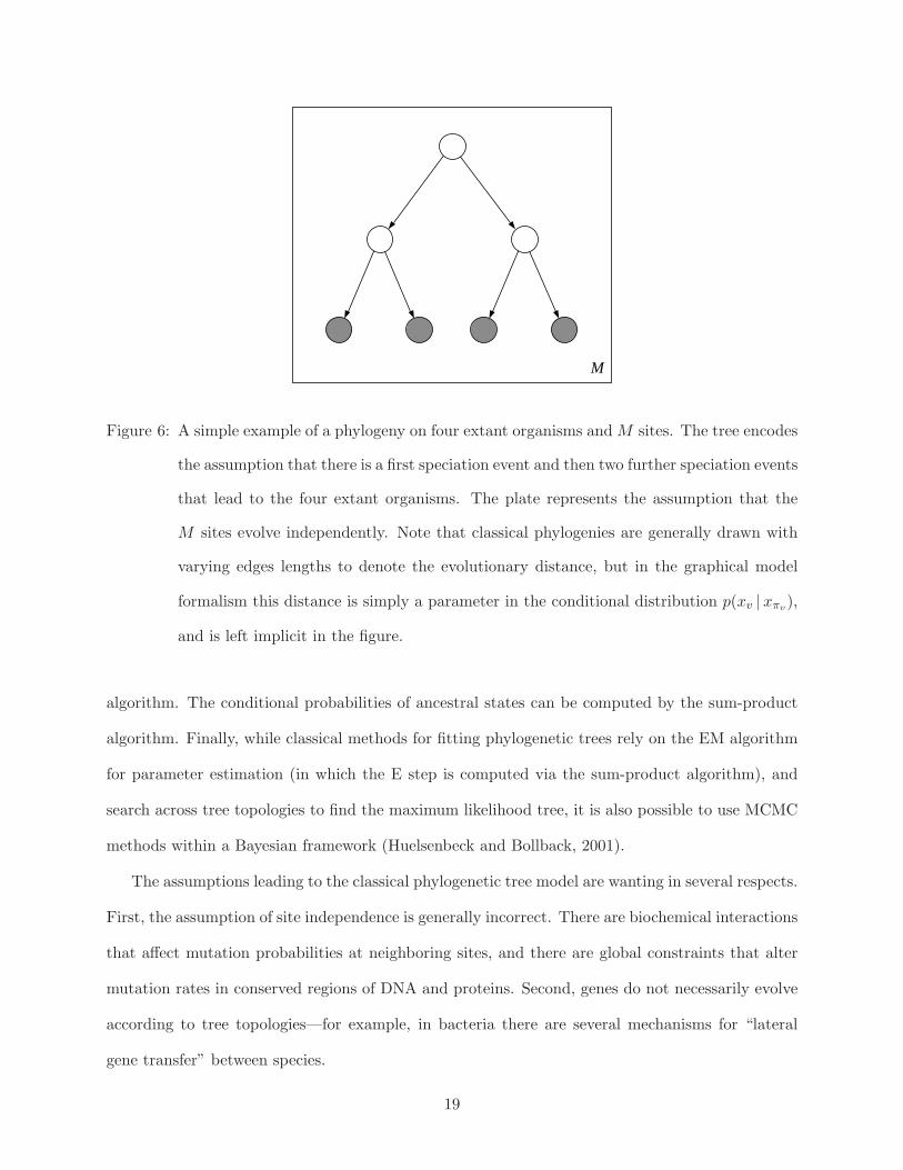
pendent, and let us begin by making that assumption. We represent a phylogeny as a binary tree

in which the leaves of the tree are the observed values of a given site in the different species and

the nonterminals are the values of the site for putative ancestral species (see Figure 6). Thus, in

the case of DNA, all of the nodes in the tree are multinomial random variables with four states,

and in the case of proteins, all nodes are multinomial with twenty states. Treating the tree as a

directed graphical model, we parameterize the tree by following the recipe in Eq. (1) and annotating

each edge with the conditional probability of a state given its ancestral state.3 These conditional

probabilities are generally parameterized in terms of an “evolutionary distance” parameter that is

to be estimated, and their parametric form is an exponential decay to an equilibrium distribution

across the four nucleotides or twenty amino acids (Felsenstein, 1981).

Taking the product of the local parameterizations, we obtain the joint probability of the states

of a given site, and taking a further product over sites (the plate in Figure 6), we obtain the joint

probability across all sites. The likelihood is easily computed via the elimination algorithm—indeed

the “pruning” algorithm of Felsenstein (1981) was an early instance of a graphical model elimination

3. In fact, the likelihood of a phylogenetic tree is generally independent of the choice of root, and the undirected

formalism is often more appropriate.

18

M

Figure 6: A simple example of a phylogeny on four extant organisms and M sites. The tree encodes

the assumption that there is a first speciation event and then two further speciation events

that lead to the four extant organisms. The plate represents the assumption that the

M sites evolve independently. Note that classical phylogenies are generally drawn with

varying edges lengths to denote the evolutionary distance, but in the graphical model

formalism this distance is simply a parameter in the conditional distribution p(xv |xπv),

and is left implicit in the figure.

algorithm. The conditional probabilities of ancestral states can be computed by the sum-product

algorithm. Finally, while classical methods for fitting phylogenetic trees rely on the EM algorithm

for parameter estimation (in which the E step is computed via the sum-product algorithm), and

search across tree topologies to find the maximum likelihood tree, it is also possible to use MCMC

methods within a Bayesian framework (Huelsenbeck and Bollback, 2001).

The assumptions leading to the classical phylogenetic tree model are wanting in several respects.

First, the assumption of site independence is generally incorrect. There are biochemical interactions

that affect mutation probabilities at neighboring sites, and there are global constraints that alter

mutation rates in conserved regions of DNA and proteins. Second, genes do not necessarily evolve

according to tree topologies—for example, in bacteria there are several mechanisms for “lateral

gene transfer” between species.

19

The graphical model formalism provides a natural upgrade path for considering more realistic

phylogenetic models that capture these phenomena. Lateral gene transfer is readily accommodated

by simply removing the restriction to a tree topology. Lack of independence between sites is

captured by replacing the plate in Figure 6 with an explicit array of graphs, one for each site,

with horizontal edges capturing interactions. For example, one could consider Markovian models

in which there are edges between ancestral nodes in neighboring sites. In general, such models

create loops in the underlying graph and approximate inference methods will generally be required.

4.2 Pedigrees and multilocus linkage analysis

While phylogenies attempt to model relationships among the instances of a single gene as found in

different species in evolutionary time, pedigrees are aimed at a finer level of granularity. A pedigree

displays the parent-child relationships within a group of organisms in a single species, and attempts

to account for the presence of variants of a gene as they flow through the population. A multilocus

pedigree is a pedigree which accounts for the flow of multiple genes. Multilocus pedigrees turn out

to be a special case of a graphical model known as a factorial hidden Markov model.

Let us briefly review the relevant genetic terminology. Arrayed along each chromosome are a set

of loci, which correspond to genes or other markers. Chromosomes occur in pairs, and thus there

are a pair of genes at each locus.4 Each gene occurs in one of several variant forms—alleles—in

the population. Thus at each locus, there is a pair of alleles. The full set of all such pairs for a

given individual is referred to as the genotype of that individual. Given the genotype, there is a

(generally stochastic) mapping to the phenotype—a set of observable traits. One often makes the

simplifying assumption that each trait is determined by a single pair of alleles, but as will be seen

our modeling formalism does not require this (generally inaccurate) assumption.

4. This is true for humans (for all but the X and Y chromosomes), but not for all organisms. The models that

we discuss can easily be specialized to organisms in which chromosomes are not paired, and in particular can

accommodate the X and Y chromosomes in humans.

20

π( )i fG π( )i mG μ( )i fG μ( )i mG

i fG imG

ifHimH

( )n ( )n ( )n ( )nP

( )nP

( )n

P( )n

( )n ( )n

( )n ( )n

π( )i

i

μ( )i

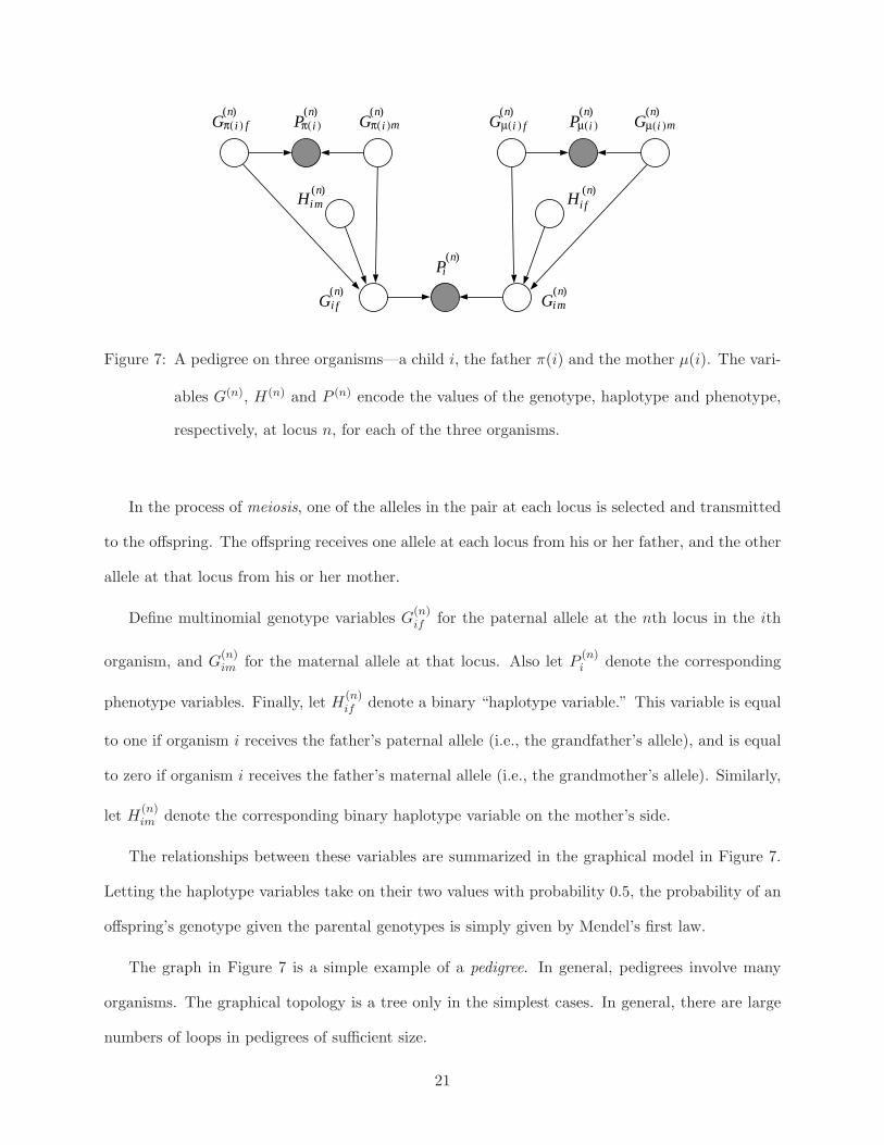
Figure 7: A pedigree on three organisms—a child i, the father π(i) and the mother μ(i). The vari-

ables G(n), H(n) and P (n) encode the values of the genotype, haplotype and phenotype,

respectively, at locus n, for each of the three organisms.

In the process of meiosis, one of the alleles in the pair at each locus is selected and transmitted

to the offspring. The offspring receives one allele at each locus from his or her father, and the other

allele at that locus from his or her mother.

Define multinomial genotype variables G(n)if for the paternal allele at the nth locus in the ith

organism, and G(n)im for the maternal allele at that locus. Also let P (n)

i denote the corresponding

phenotype variables. Finally, let H(n)if denote a binary “haplotype variable.” This variable is equal

to one if organism i receives the father’s paternal allele (i.e., the grandfather’s allele), and is equal

to zero if organism i receives the father’s maternal allele (i.e., the grandmother’s allele). Similarly,

let H(n)im denote the corresponding binary haplotype variable on the mother’s side.

The relationships between these variables are summarized in the graphical model in Figure 7.

Letting the haplotype variables take on their two values with probability 0.5, the probability of an

offspring’s genotype given the parental genotypes is simply given by Mendel’s first law.

The graph in Figure 7 is a simple example of a pedigree. In general, pedigrees involve many

organisms. The graphical topology is a tree only in the simplest cases. In general, there are large

numbers of loops in pedigrees of sufficient size.

21

mH( )ni

fH( )ni

mHi

fHi( )n+1

( )n+1

G( )n

P( )n

G( )n+1

P( )n+1

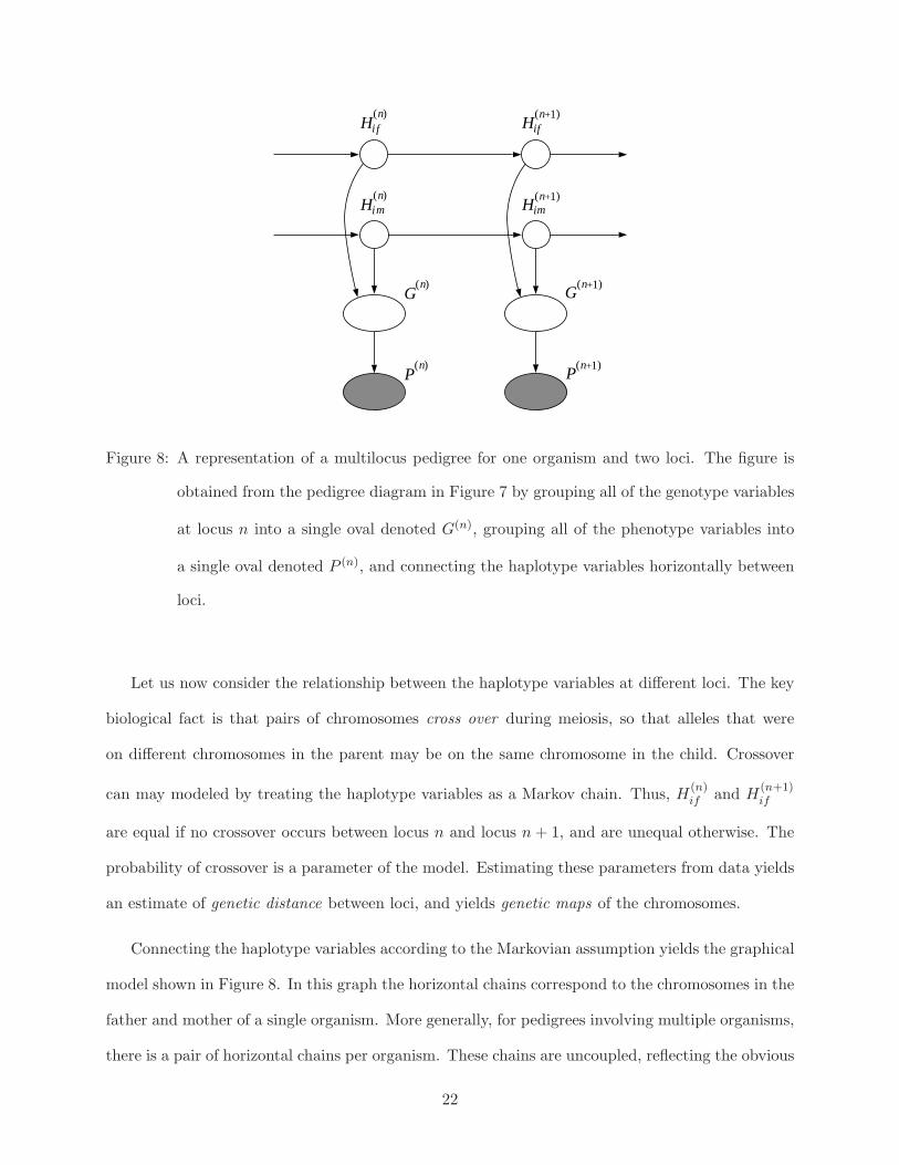
Figure 8: A representation of a multilocus pedigree for one organism and two loci. The figure is

obtained from the pedigree diagram in Figure 7 by grouping all of the genotype variables

at locus n into a single oval denoted G(n), grouping all of the phenotype variables into

a single oval denoted P (n), and connecting the haplotype variables horizontally between

loci.

Let us now consider the relationship between the haplotype variables at different loci. The key

biological fact is that pairs of chromosomes cross over during meiosis, so that alleles that were

on different chromosomes in the parent may be on the same chromosome in the child. Crossover

can may modeled by treating the haplotype variables as a Markov chain. Thus, H(n)if and H

(n+1)if

are equal if no crossover occurs between locus n and locus n+ 1, and are unequal otherwise. The

probability of crossover is a parameter of the model. Estimating these parameters from data yields

an estimate of genetic distance between loci, and yields genetic maps of the chromosomes.

Connecting the haplotype variables according to the Markovian assumption yields the graphical

model shown in Figure 8. In this graph the horizontal chains correspond to the chromosomes in the

father and mother of a single organism. More generally, for pedigrees involving multiple organisms,

there is a pair of horizontal chains per organism. These chains are uncoupled, reflecting the obvious

22

fact that meiosis is independent among different organisms. The coupling among organisms is

restricted to couplings among the G(n)i variables (these couplings are contained in the ovals in

Figure 8; they have been suppressed to simplify the diagram).

The model in Figure 8 is an instance of a graphical model family known as a factorial hidden

Markov model (fHMM) (Ghahramani and Jordan, 1996); see Figure 10(c) for a generic example.

Classical algorithms for inference on multilocus pedigrees are variants of the elimination algorithm

on this fHMM, and correspond to different choices of elimination order (Lander and Green, 1987,

Elston and Stewart, 1971). While these algorithms are viable for small problems, exact inference

is intractable for general multilocus pedigrees. Indeed, focusing only on the haplotype variables,

it can be verified that the treewidth is bounded below by the number of organisms, and thus

the computational complexity is exponential in the number of organisms. More recently, Gibbs

sampling methods have been studied; in particular, Thomas et al. (2000) have proposed a blocking

Gibbs sampler that takes advantage of the graphical structure in Figure 8. Ghahramani and

Jordan (1996) presented a suite of variational and Gibbs sampling algorithms for fHMMs, and

further developments are presented by Murphy (2002).

5. Error-control codes

Graphical models play an important role in the modern theory of error-control coding. Ties between

graphs and codes were explored in the early sixties by Gallager (1963), but this seminal line of

research was largely forgotten, due at least in part to a lack of sufficiently powerful computational

tools. A flurry of recent work, however, has built on Gallager’s work and shown that surprisingly

effective codes can be built from graphical models. Codes based on graphical models are now the

most effective codes known for many channels, achieving rates near the Shannon capacity.

The basic problem of error-control coding is that of transmitting a message (a sequence of bits)

through a noisy channel, in such a way that a receiver can recover the original message despite

the noise. In general, this is achieved by transmitting additional (redundant) bits in addition to

the original message sequence. The receiver uses the redundancy to detect, and possibly correct,

23

any corruption of the message due to the noise. The key problems are that of deciding the overall

mapping between messages and the redundant bits (the problem of code design), that of computing

the redundant bits for any given message (the encoding problem), and that of estimating the original

message based on a transmitted message (the decoding problem).

There are three ways in which probability enters into the problem. First, the set of possible

messages (the source) is given a prior distribution. We will treat this distribution as uniform,

assuming in essence that a source code has been developed that extracts the statistical redundancy

from the source (this redundancy is distinct from the redundancy that we wish to impose on the

the message, a redundancy which is designed to be appropriate for a given channel). Second, the

channel is noisy. A simple example of a channel model is a binary symmetric channel (BSC), in

which each message bit is transmitted correctly (with probability α) or flipped (with probability

1−α). These transmission events are often assumed IID across the bits in a message sequence; that

is, the channel is often assumed to be memoryless. We make that assumption here for simplicity,

but it will be clear that the graphical model formalism can readily cope with non-memoryless

channels.

Finally, the code itself is often taken to be random. In the graphical model setting, in which an

instance of a code is identified with a graph, this means that we are considering random ensembles

of graphs. This assumption is not an inherent feature of the problem; rather it is imposed to allow

probabilistic tools to be applied to theoretical analysis of the properties of a code (see below).

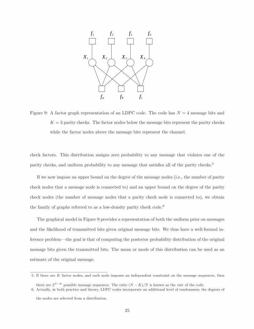
In Figure 9, we show a specific example of a graph from an ensemble known as a low-density

parity check (LDPC) code. The variable nodes in the graph are binary-valued, and represent the

message bits; a message is a specific instance of the 2N possible states of these nodes. The factor

nodes above the message nodes represent the channel. Thus, for the message variable Xi, the

factor node fi represents the likelihood p(yi |xi), where yi is the observed value of the transmitted

message. The factor nodes below the message nodes are parity-check nodes; these are equal to one

only if and only if an even number of the nodes that they are connected to are equal to one. The

prior probability distribution on messages is obtained as an instance of Eq. (3) based on the parity

24

1X 2X 3X X 4

fa fb fc

1f 2f 3f f4

Figure 9: A factor graph representation of an LDPC code. The code has N = 4 message bits and

K = 3 parity checks. The factor nodes below the message bits represent the parity checks

while the factor nodes above the message bits represent the channel.

check factors. This distribution assigns zero probability to any message that violates one of the

parity checks, and uniform probability to any message that satisfies all of the parity checks.5

If we now impose an upper bound on the degree of the message nodes (i.e., the number of parity

check nodes that a message node is connected to) and an upper bound on the degree of the parity

check nodes (the number of message nodes that a parity check node is connected to), we obtain

the family of graphs referred to as a low-density parity check code.6

The graphical model in Figure 9 provides a representation of both the uniform prior on messages

and the likelihood of transmitted bits given original message bits. We thus have a well-formed in-

ference problem—the goal is that of computing the posterior probability distribution of the original

message bits given the transmitted bits. The mean or mode of this distribution can be used as an

estimate of the original message.

5. If there are K factor nodes, and each node imposes an independent constraint on the message sequences, then

there are 2N−K possible message sequences. The ratio (N − K)/N is known as the rate of the code.6. Actually, in both practice and theory, LDPC codes incorporate an additional level of randomness; the degrees of

the nodes are selected from a distribution.

25

While in principle any of the inference algorithms associated with general graphical models

could be used for LDPC codes, the presence of loops in the graph, and the large scale of graphs

that are used (in which N may be as large as many tens of thousands) rules out exact inference.

Moreover, MCMC algorithms do not appear to be viable in this domain. The algorithm that is

used in practice is the sum-product algorithm. The algorithm is quite successful in practice for

large block lengths (large values of N). Moreover, theoretical convergence results are available for

the sum-product algorithm in this setting (Richardson et al., 2001). Averaging over the ensemble

of graphs, it can be shown that the average error probability goes to zero over the iterations of

the sum-product algorithm, given conditions on the channel, the degree distributions, the block

length and the code rate. Also, a martingale argument can be invoked to show that almost all

codes behave like the average code, which justifies the random selection of a specific code from the

ensemble for use in practice.

Graphical models continue to play a central role in the development of error-control codes.

New codes are designed by proposing alternative graphical structures, and the analysis of decoding

performance makes direct use of the graphical structure. The graphical framework allows the

exploration of more complex channel models (for example, the factor nodes representing the channel

can connect to multiple message nodes in Figure 9 in the case of channels with memory).

6. Speech, language and information retrieval

The fields of speech recognition, natural language processing and information retrieval involve the

study of complex phenomena that exhibit many kinds of structural relationships. Graphical models

play an increasingly important role in attempts to model these phenomena and extract information

that is needed in a given problem domain.

6.1 Markov and hidden Markov models

Markov models and hidden Markov models are graphical models that attempt to capture some

of the simplest sequential structure inherent in speech and language. In both cases the graphical

26

model is a chain of multinomial “state” nodes Xt, with links between these nodes parameterized by

a state transition matrix. In the case of a first-order Markov model, there is an edge between state

Xt−1 and state Xt, for t ∈ {1, . . . T}, while in higher-order Markov models there are edges from

earlier states Xt−τ . Hidden Markov models (HMMs) have an additional set of “output” nodes Yt,

with edges between Xt and Yt.

A simple yet important application of HMMs arises in the part-of-speech problem. In this

problem, the data are word sequences, and the goal is to tag the words according to their part of

speech (noun, verb, preposition, etc.). Thus the states Xt take as many values as there are parts

of speech (typically several dozen), and the outputs Yt take as many values as there are words

in the vocabulary (typically many tens of thousands). Training data generally consist of “tagged

data”—(Xt, Yt) pairs—and the subsequent inference problem is that of inferring a sequence of Xt

values given a sequence of Yt values.

Speech recognition provides a wide-ranging set of examples of the application of HMMs. In this

setting, the observables Yt are generally short-term acoustic spectra, either continuous-valued or

discretized. A single HMM is often designed to cover a small phonetic unit of speech such as a

syllable or diphone, and the states Xt are generally treated as unobserved (latent) variables. A

library of such HMMs is created based on a corpus of training data. The HMMs in this library

are then assembled into a lattice, which is itself a large graphical model that has edges between

each of the elemental HMMs. The inference problem in this lattice of HMMs is generally that of

finding the mode of the posterior distribution on state sequences, a computation which effectively

segments a long observation sequence into its component speech units.

The elemental HMMs in this lattice are often trained based on “segmented data,” in which the

portion of the speech sequence appropriate to each HMM is known in advance. It is also necessary

to estimate the parameters associated with the transitions between the speech units, a problem

known as language modeling. In this setting, Markov models are widely used. In particular, it is

generally necessary to provide an estimate of the probability of a given word based on the previous

two words (a “trigram model”). Given the large number of words in the vocabulary, this involves

27

a large number of parameters relative to the amount of available data, and fully Bayesian methods

(or adhoc “smoothing” techniques) are generally necessary for parameter estimation.

Finally, returning briefly to bioinformatics, it is worth noting that HMMs have a large number of

applications in bioinformatics, including the problems of gene-finding in DNA and domain modeling

in proteins. See Durbin et al. (1998) for a discussion of these applications.

6.2 Variations on Markovian models

A large number of variations on Markovian models are currently being explored in the fields of

speech and language processing, and also in bioinformatics. Many of these models are readily seen

to be members of the larger family of graphical models.

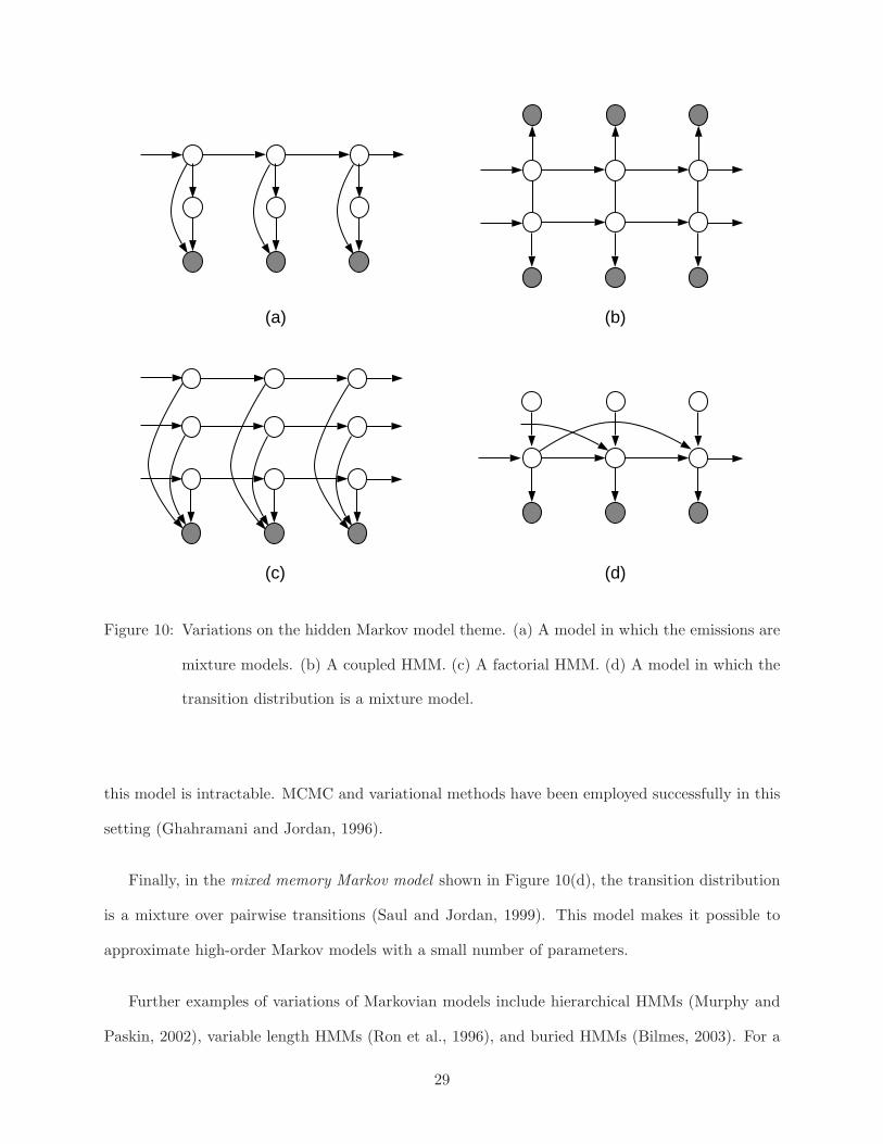
In speech recognition models, the state-to-output distribution, p(yt |xt), is commonly taken to

be a mixture of Gaussians, reflecting the multimodality that is commonly observed in practice. As

shown in Figure 10(a), this can be represented as a graphical model in which additional (multino-

mial) variables are introduced to encode the allocations of the mixture components. The model

remains eminently tractable for exact inference.

A more serious departure is the coupled hidden Markov model shown in Figure 10(b) (Saul

and Jordan, 1995). This model involves two chains of state variables which are coupled via links

between the chains.7 Triangulating this graph yields cliques of size three, and the model remains

tractable for exact inference.

More generally, the factorial hidden Markov model shown in Figure 10(c) is an instance of model

involving multiple chains (Ghahramani and Jordan, 1996). In this particular model the states are

coupled only via their connection to a common set of output variables (but variations can also be

considered in which there are links among the chains). The factorial HMM allows large state spaces

to be represented with a small number of parameters. Note that triangulation of this model yields

cliques of size M + 1, where M is the number of chains, and thus for even moderate values of M

7. The model is a hybrid of the directed and undirected formalisms; an instance of the family of chain graphs (Lau-

ritzen, 1996).

28

(a) (b)

(c) (d)

Figure 10: Variations on the hidden Markov model theme. (a) A model in which the emissions are

mixture models. (b) A coupled HMM. (c) A factorial HMM. (d) A model in which the

transition distribution is a mixture model.

this model is intractable. MCMC and variational methods have been employed successfully in this

setting (Ghahramani and Jordan, 1996).

Finally, in the mixed memory Markov model shown in Figure 10(d), the transition distribution

is a mixture over pairwise transitions (Saul and Jordan, 1999). This model makes it possible to

approximate high-order Markov models with a small number of parameters.

Further examples of variations of Markovian models include hierarchical HMMs (Murphy and

Paskin, 2002), variable length HMMs (Ron et al., 1996), and buried HMMs (Bilmes, 2003). For a

29

N

nZα

β

θ nW

M

Figure 11: The latent Dirichlet allocation model for document collections. The outer plate repre-

sents a corpus containing M documents, while the inner plate represents an N -word

document within that corpus.

recent overview of these models in the context of applications to speech and language problems,

see Bilmes (2003).

6.3 A hierarchical Bayesian model for document collections

For large-scale collections of documents (such as the World Wide Web), it is generally computa-

tionally infeasible to attempt to model the sequential structure of individual documents, and the

field of information retrieval is generally built on the “bag-of-words” assumption—the assumption

that word order within a document can be neglected for the purposes of indexing and retrieving

documents. This is simply an assumption of exchangeability, and leads (via the de Finetti theorem)

to the consideration of latent variable models for documents.

While neglecting sequential structure, it may be desirable to attempt to capture other kinds of

statistical structure in document collections, in particular the notion that documents are character-

ized by topics. Blei et al. (2002) have proposed a hierarchical latent variable model that has explicit

representations for documents, topics and words. The model is shown in Figure 11. Words are

represented by a multinomial variable W and topics are represented by a multinomial variable Z.

Generally the cardinality of Z is significantly smaller than that of W . As shown by the innermost

30

plate, the M words in a document are generated by repeatedly choosing a topic variable and then

choosing a word corresponding to that topic. The probabilities of the topics are document-specific,

and they are assigned via the value of a Dirichlet random variable θ. As shown by the outermost

plate, this variable is sampled once for each of the N documents in the corpus. As this example

demonstrates, the graphical model formalism is useful in the design of a wide variety of mixed

effects models and hierarchical latent variable models.

7. Discussion

Let us close with a few remarks on the present and future of graphical models in statistics. Until

very recently, graphical models have been relegated to the periphery in statistics, viewed as useful

in specialized situations but not a central theme. Several factors are responsible for their increas-

ing prominence. First, hierarchical Bayesian models are naturally specified as directed graphical

models, and the ongoing interest in the former has raised the visibility of the latter. Second,

graph-theoretic concepts are key in recent attempts to provide theoretical guarantees for MCMC

algorithms. Third, a increasing awareness of the importance of graph-theoretic representations of

probability distributions in fields such as statistical and quantum physics, bioinformatics, signal

processing, econometrics and information theory has accompanied a general increase in interest in

applications of statistics. Finally, the realization that seemingly specialized methods developed in

these disciplines are instances of a general class of variational inference algorithms has led to an

increasing awareness that there may be alternatives to MCMC for general statistical inference that

are worth exploring.

While the links to graph theory and thence to computational issues are a major virtue of the

graphical model formalism, there is much that is still lacking. In the setting of large-scale graphical

models, one would like to have some general notion of a tradeoff between computation and accuracy

on which to base choices in model specification and the design of inference algorithms. Such a

tradeoff is of course missing not only in the graphical model formalism but in statistics at large.

Taking a decision-theoretic perspective, we should ask that our loss functions reflect computational

31

complexity as well as statistical fidelity. By having a foot in both graph theory and probability

theory, graphical models may provide hints as to how to proceed if we wish to aim at a further and

significantly deeper linkage of statistical science and computational science.

References

Aji, S. M. and McEliece, R. J. (2000). The generalized distributive law. IEEE Transactions on

Information Theory 46 325–343.

Arnborg, S., Corneil, D. G., and Proskurowski, A. (1987). Complexity of finding embeddings

in a k-tree. SIAM Journal on Algebraic and Discrete Methods 8 277–284.

Attias, H. (2000). A variational Bayesian framework for graphical models. In Advances in Neural

Information Processing Systems 12, MIT Press, Cambridge, MA.

Bilmes, J. (2003). Graphical models and automatic speech recognition. In Mathematical Founda-

tions of Speech and Language Processing, Springer-Verlag, New York, NY.

Blei, D. M., Jordan, M. I., and Ng, A. Y. (2002). Hierarchical Bayesian models for applications

in information retrieval. In Bayesian Statistics 7, Oxford University Press, Oxford.

Brown, L. (1986). Fundamentals of Statistical Exponential Families. Institute of Mathematical

Statistics, Hayward, CA.

Cowell, R. G., Dawid, A. P., Lauritzen, S. L., and Spiegelhalter, D. J. (1999). Probabilistic

Networks and Expert Systems. Springer, New York, NY.

Durbin, R., Eddy, S., Krogh, A., and Mitchison, G. (1998). Biological Sequence Analysis.

Cambridge University Press, Cambridge.

Elston, R. C. and Stewart, J. (1971). A general model for the genetic analysis of pedigree data.

Human Heredity 21 523–542.

32

Felsenstein, J. (1981). Evolutionary trees from DNA sequences: a maximum likelihood approach.

Journal of Molecular Evolution 17 368–376.

Gallager, R. G. (1963). Low-Density Parity Check Codes. MIT Press, Cambridge, MA.

Ghahramani, Z. and Beal, M. (2001). Propagation algorithms for variational Bayesian learning.

In Advances in Neural Information Processing Systems 13, MIT Press, Cambridge, MA.

Ghahramani, Z. and Jordan, M. I. (1996). Factorial hidden Markov models. Machine Learning

37 183–233.

Gilks, W., Thomas, A., and Spiegelhalter, D. (1994). A language and a program for complex

Bayesian modelling. The Statistician 43 169–178.

Huelsenbeck, J. P. and Bollback, J. P. (2001). Empirical and hierarchical Bayesian estimation

of ancestral states. Systematic Biology 50 351–366.

Jensen, C. S., Kong, A., and Kjaerulff, U. (1995). Blocking-Gibbs sampling in very large

probabilistic expert systems. International Journal of Human-Computer Studies 42 647–666.

Jordan, M. I., editor (1999). Learning in Graphical Models. MIT Press, Cambridge, MA.

Jordan, M. I., Ghahramani, Z., Jaakkola, T. S., and Saul, L. K. (1999). Introduction to

variational methods for graphical models. Machine Learning 37 183–233.

Kschischang, F., Frey, B. J., and Loeliger, H.-A. (2001). Factor graphs and the sum-product

algorithm. IEEE Transactions on Information Theory 47 498–519.

Lander, E. S. and Green, P. (1987). Construction of multilocus genetic maps in humans. Pro-

ceedings of the National Academy of Sciences 84 2363–2367.

Lauritzen, S. L. (1996). Graphical Models. Clarendon Press, Oxford.

33

Leisink, M. A. R. and Kappen, H. J. (2002). General lower bounds based on computer generated

higher order expansions. In Uncertainty in Artificial Intelligence, Morgan Kaufmann, San Mateo,

CA.

Liu, J. (2001). Monte Carlo Strategies in Scientific Computing. Springer, New York, NY.

Minka, T. (2002). A family of algorithms for approximate Bayesian inference. PhD thesis, Mas-

sachusetts Institute of Technology.

Murphy, K. (2002). Dynamic Bayesian Networks: Representation, Inference and Learning. PhD

thesis, University of California, Berkeley.

Murphy, K. and Paskin, M. (2002). Linear time inference in hierarchical HMMs. In Advances in

Neural Information Processing Systems 13, MIT Press, Cambridge, MA.

Pearl, J. (1988). Probabilistic Reasoning in Intelligent Systems: Networks of Plausible Inference.

Morgan Kaufmann, San Mateo, CA.

Richardson, S., Leblond, L., Jaussent, I., and Green, P. J. (2002). Mixture models in

measurement error problems, with reference to epidemiological studies. Biostatistics (submitted).

Richardson, T., Shokrollahi, A., and Urbanke, R. (2001). Design of provably good low-

density parity check codes. IEEE Transactions on Information Theory 47 619–637.

Robert, C. and Casella, G. (2004). Monte Carlo Statistical Methods. Springer, New York, NY.

Rockafellar, G. (1970). Convex Analysis. Princeton University Press, Princeton, NJ.

Ron, D., Singer, Y., and Tishby, N. (1996). The power of amnesia: Learning probabilistic

automata with variable memory length. Machine Learning 25 117–149.

Saul, L. K. and Jordan, M. I. (1995). Boltzmann chains and hidden Markov models. In Advances

in Neural Information Processing Systems 7, MIT Press, Cambridge, MA.

34

Saul, L. K. and Jordan, M. I. (1999). Mixed memory Markov models: Decomposing complex

stochastic processes as mixture of simpler ones. Machine Learning 37 75–87.

Shenoy, P. and Shafer, G. (1990). Axioms for probability and belief-function propagation. In

Uncertainty in Artificial Intelligence, Morgan Kaufmann, San Mateo, CA.

Tatikonda, S. and Jordan, M. I. (2002). Loopy belief propagation and Gibbs measures. In

Uncertainty in Artificial Intelligence, Morgan Kaufmann, San Mateo, CA.

Thomas, A., Gutin, A., Abkevich, V., and Bansal, A. (2000). Multilocus linkage analysis by

blocked Gibbs sampling. Statistics and Computing 10 259–269.

Wainwright, M. J. and Jordan, M. I. (2003). Graphical models, exponential families, and

variational inference. Technical Report 649, Department of Statistics, University of California,

Berkeley.

Wainwright, M. J. and Jordan, M. I. (2004). Semidefinite relaxations for approximate inference

on graphs with cycles. In Advances in Neural Information Processing Systems 16, MIT Press,

Cambridge, MA.

Yedidia, J., Freeman, W., and Weiss, Y. (2001). Generalized belief propagation. In Advances

in Neural Information Processing Systems 13, MIT Press, Cambridge, MA.

35