Global description of patterns far from onset: a case...

Physica D 184 (2003) 127–140

Global description of patterns far from onset: a case study

N. Ercolania, R. Indika,∗, A.C. Newella, T. Passotba Department of Mathematics, University of Arizona, Tucson, AZ 85721, USA

b CNRS, Observatoire de la Cˆote d’Azur, B.P. 4229, 06304 Nice Cedex 4, France

Abstract

The Cross–Newell phase diffusion equationτ(k)ΘT = −∇ · kB(k), k = ∇Θ, |k| = k, and its regularization describepatterns and defects far from onset in large aspect ratio systems with translational and rotational symmetry. In this paper weshow how director field solutions of this equation can be used to describe features of global patterns. The ideas are illustratedin the context of a non-trivial case study of high Prandtl number convection in a large aspect ratio, shallow, elliptical containerwith heated sidewalls, for which we also have the results of simulation and experiment.© 2003 Elsevier B.V. All rights reserved.

Keywords:Patterns; Defects; Convection

1. Introduction

A macroscopic description of convection patternsfar from the onset of the convective instability stillpresents a considerable challenge for both physicistsand mathematicians. The path we have followed totackle this problem is to study the phase diffusionequation that results from the elimination of the com-plex three-dimensional structure of the microscopicroll pattern and that focuses on the large-scale dy-namics of the phase gradient, which is perpendicularto the rolls.

We recently established[1] rigorous proofs for theexistence and form of solutions to the regularizedphase diffusion equation in the limit where the in-verse aspect ratioε (ratio of the roll wavelength tothe typical size of the container) goes to zero. Thebasis of this work was first to remark that solving thephase diffusion equation amounts to solving a mini-

∗ Corresponding author.E-mail address:[email protected] (R. Indik).

mization problem for an energyE which is the sumof two terms, one associated with roll bending andthe other with the mismatch between the local andthe preferred wave number. Generally pattern form-ing systems are not gradient flows. However in thehigh Prandtl number limit the Oberbeck–Boussinesqequations behave as if they were[2]. A second pointwas to study a separate, although closely related,problem defined by equating the two components ofthe energy. Thisself-dual reductionleads to solu-tions which are also solutions of the original phasediffusion equation when the Gaussian curvature ofthe graph of the phase vanishes. For many of theobserved structures in patterns, the curvature doesvanish except in the neighborhood of certain pointsor curves. In general, however, the solutions of theself-dual equations are not solutions of this phaseequation but they do provide, for eachε, an up-per bound on the energy. The remarkable point isthat, for a model form of the phase equation validwhen the wave number is everywhere close to theselected one, the self-dual equation can be linearized

0167-2789/$ – see front matter © 2003 Elsevier B.V. All rights reserved.doi:10.1016/S0167-2789(03)00217-3

128 N. Ercolani et al. / Physica D 184 (2003) 127–140

and leads to explicit solutions whose limits asε goesto zero, are well controlled. In special cases, a lowerbound for the energy can be found, that equals theupper bound and thus provides an explicit minimizer(not necessarily unique).

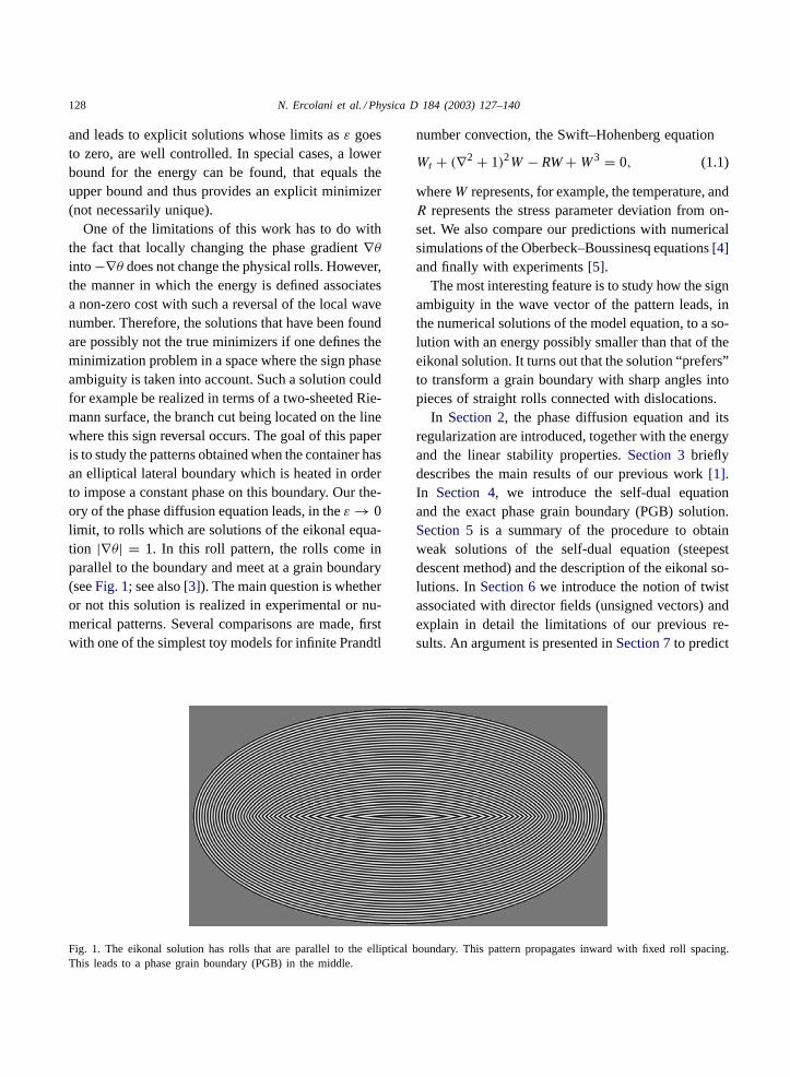
One of the limitations of this work has to do withthe fact that locally changing the phase gradient∇θinto −∇θ does not change the physical rolls. However,the manner in which the energy is defined associatesa non-zero cost with such a reversal of the local wavenumber. Therefore, the solutions that have been foundare possibly not the true minimizers if one defines theminimization problem in a space where the sign phaseambiguity is taken into account. Such a solution couldfor example be realized in terms of a two-sheeted Rie-mann surface, the branch cut being located on the linewhere this sign reversal occurs. The goal of this paperis to study the patterns obtained when the container hasan elliptical lateral boundary which is heated in orderto impose a constant phase on this boundary. Our the-ory of the phase diffusion equation leads, in theε→ 0limit, to rolls which are solutions of the eikonal equa-tion |∇θ| = 1. In this roll pattern, the rolls come inparallel to the boundary and meet at a grain boundary(seeFig. 1; see also[3]). The main question is whetheror not this solution is realized in experimental or nu-merical patterns. Several comparisons are made, firstwith one of the simplest toy models for infinite Prandtl

Fig. 1. The eikonal solution has rolls that are parallel to the elliptical boundary. This pattern propagates inward with fixed roll spacing.This leads to a phase grain boundary (PGB) in the middle.

number convection, the Swift–Hohenberg equation

Wt + (∇2 + 1)2W − RW+W3 = 0, (1.1)

whereW represents, for example, the temperature, andR represents the stress parameter deviation from on-set. We also compare our predictions with numericalsimulations of the Oberbeck–Boussinesq equations[4]and finally with experiments[5].

The most interesting feature is to study how the signambiguity in the wave vector of the pattern leads, inthe numerical solutions of the model equation, to a so-lution with an energy possibly smaller than that of theeikonal solution. It turns out that the solution “prefers”to transform a grain boundary with sharp angles intopieces of straight rolls connected with dislocations.

In Section 2, the phase diffusion equation and itsregularization are introduced, together with the energyand the linear stability properties.Section 3brieflydescribes the main results of our previous work[1].In Section 4, we introduce the self-dual equationand the exact phase grain boundary (PGB) solution.Section 5is a summary of the procedure to obtainweak solutions of the self-dual equation (steepestdescent method) and the description of the eikonal so-lutions. InSection 6we introduce the notion of twistassociated with director fields (unsigned vectors) andexplain in detail the limitations of our previous re-sults. An argument is presented inSection 7to predict

N. Ercolani et al. / Physica D 184 (2003) 127–140 129

the critical angle at which a PGB becomes unsta-ble towards the formation of dislocations.Sections 8and 9, respectively, describe the numerical simulationsof the Swift–Hohenberg equation and the compar-isons with simulations of the Oberbeck–Boussinesqequation and laboratory experiments. Some conclud-ing remarks are made inSection 10.

2. Background

Let us consider a straight roll solution of theOberbeck–Boussinesq[6], or the Swift–Hohenberg(SH) equations, of the form

w(x, y, t) = F(θ) = ΣAn(k) cosnθ. (2.1)

F(θ) is a 2π periodic function of a phaseθ whose gra-dient k is the constant wave vector of the pattern. Animportant point, related to the question of twist dis-cussed inSection 6, is to remark that the microscopicfield is unchanged on the reversal ofθ, θ → −θ. Next,we seek nearby solutions in the form

w(x, y, t) = F(

1

εΘ

)+ εw1 + ε2w2 + · · · (2.2)

for which the local phaseΘ varies over large spatialand temporal scales defined asX = εx, T = ε2t. Inparticular, the wave vectork = ∇θ = ∇XΘ = (f, g),changes by order 1 over distances of(1/ε)λ, whereλ is the wavelength andε,0 < ε 1 is the inverseaspect ratio of the system. For the modulated solution,the amplitudesAn are still slaved to the local wavenumberk = |∇θ| via An = An(k).

Because the original system is translationally invari-ant, the variation ofw aboutF(θ) has a non-trivial nullspace and the non-homogeneous equation for the cor-rectionsw1, w2, . . . to F(θ) must satisfy solvabilityconditions. These express the fact that the right-handsides of these equations must lie in the range of thelinear operator obtained by linearizingw about the ex-act solutionF(θ). To dominant order inε [7],

τ(k)ΘT = −∇ · kB(k). (2.3)

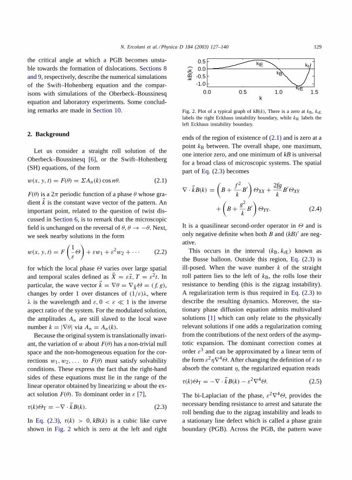
In Eq. (2.3), τ(k) > 0, kB(k) is a cubic like curveshown in Fig. 2 which is zero at the left and right

kB

kr

krE

klE

0.0 0.5 1.0 1.5k

-1.0-0.50.00.5

kB(k

)

Fig. 2. Plot of a typical graph ofkB(k), There is a zero atkB, krElabels the right Eckhaus instability boundary, whileklE labels theleft Eckhaus instability boundary.

ends of the region of existence of(2.1)and is zero at apoint kB between. The overall shape, one maximum,one interior zero, and one minimum ofkB is universalfor a broad class of microscopic systems. The spatialpart ofEq. (2.3)becomes

∇ · kB(k) =(B + f 2

kB′)ΘXX + 2fg

kB′ΘXY

+(B + g2

kB′)ΘYY. (2.4)

It is a quasilinear second-order operator inΘ and isonly negative definite when bothB and(kB)′ are neg-ative.

This occurs in the interval(kB, krE) known asthe Busse balloon. Outside this region,Eq. (2.3) isill-posed. When the wave numberk of the straightroll pattern lies to the left ofkB, the rolls lose theirresistance to bending (this is the zigzag instability).A regularization term is thus required inEq. (2.3)todescribe the resulting dynamics. Moreover, the sta-tionary phase diffusion equation admits multivaluedsolutions[1] which can only relate to the physicallyrelevant solutions if one adds a regularization comingfrom the contributions of the next orders of the asymp-totic expansion. The dominant correction comes atorderε3 and can be approximated by a linear term ofthe formε2η∇4Θ. After changing the definition ofε toabsorb the constantη, the regularized equation reads

τ(k)ΘT = −∇ · kB(k)− ε2∇4Θ. (2.5)

The bi-Laplacian of the phase,ε2∇4Θ, provides thenecessary bending resistance to arrest and saturate theroll bending due to the zigzag instability and leads toa stationary line defect which is called a phase grainboundary (PGB). Across the PGB, the pattern wave


vector k changes abruptly (over distances of the rollwavelength).

Considering a compact domainΩ with smoothboundary, one easily finds thatEq. (2.5)is essentiallya gradient flow

τ(k)ΘT = − δFδΘ

(2.6)

with

F [Θ] =∫Ω

(1

2G2(k)+ 1

2ε2(∇2Θ)2

)dX, (2.7)

and

G2(k) = −2∫ k

kB

kB(k)dk. (2.8)

In F [Θ], theG2 term is zero whenk = kB, the pre-ferred wave number. It represents the wave numbermismatch energy density while theε2(∇2Θ)2 termrepresents the bending energy density. The systemwould like to relax to the state wherek = kB every-where. In interesting circumstances, such as the prob-lem posed inSection 1, this cannot be the case andpatches of planform wherek = kB are mediated byline and point defects.

Before analyzing the minimization problem forthe energy(2.7), we emphasize the sense in whichequation (2.5)is universal. First, we have assumedthat there are no other slow modes than the one asso-ciated with the translational invariance of the system.In particular, we exclude cases (such as in small tomoderate Prandtl number convection) where a meanflow, driven by roll curvature gradients, is present.Second, we have assumed that noshort scaleinsta-bility (e.g. a cross-roll instability) can develop andtrigger a modification to the local roll planform.

3. Description of asymptotic minimizers for RCN

For k close tokB, G2 is approximated to secondorder by(k2 − k2

B)2. ChoosingkB = 1, the RCN (reg-

ularized Cross–Newell) free energy divided byε be-comes

Eε[Θ] =∫Ω

(ε(∇ · k)2 + 1

ε(k2 − 1)2

)dX. (3.1)

Our goal is to study the asymptotic form, asε → 0,of the minimizersΘε of Eε[Θ] within the family oflocally gradient vector fieldsk = ∇Θ for which thephaseΘ belongs to the class

Aε=Θ ∈ H2(Ω);Θ

∣∣∣∣Ω=αε(s), ∂Θ∂n

∣∣∣∣Ω

= βε(s),

(3.2)

whereαε(s) andβε(s) are two sequences of smoothbounded functions of the boundary arclengths whichare, respectively, uniformly convergent inε.

The energy associated with the variational prob-lem (3.1) has the form of the well-known Ginzburg–Landau functional[1]. The difference is that in theRCN variational problem this energy is restricted tovector fields which are gradient. We are able to saysomething about the asymptotic limit of these mini-mizers, in the class ofAε coming from Dirichlet vis-cosity boundary conditions (these will be described inthe next section). We summarize here what is knownabout this limit.

Theorem 3.1.

(a) As ε → 0, the minimizersΘε → Θ0 in H1(Ω),whereΘ0 solves the eikonal equation|∇Θ0| =1. Defects are, therefore, supported on locallyone-dimensional sets which are a union of locallyrectifiable curves. LetΣ denote this total defectlocus.

(b) The asymptotic minimal energy is bounded:

lim infε→0E(Θε) ≤ 1

3

∫Σ

|[∇Θ0]|3 ds,

where[∇Θ0] is the jump ink0 acrossΣ and dsis the element of arclength.

(c) In the class of cases whenΣ is a single straightline segment, the previous inequality becomes anequality; i.e., the upper bound is tight.

Details about the proofs of these results may befound in[1]. In that work we show thatΘε convergesweakly toΘ0; however, more recent results on thesetypes of minimization problems[8–10] enable one toimprove this to the strong convergence stated above.


We will construct some explicit examples of eikonalsolutions inSection 5.

These one-dimensional defect loci are what wehave calledphase grain boundaries. Our bound on theasymptotic minimum energy indicates that the bendingterm

∫Ω

|∇k|2 in this free energy will diverge as 1/ε.This is a major increase in energetic cost comparedto the log(1/ε) cost of the original Ginzburg–Landauproblem whose defects are point vortices. We reit-erate that this difference is due to the fact that, incomparison to Ginzburg–Landau, the minimizationfor RCN is done over the smaller class of irrotationalvector fields; i.e., thosek which are gradient.

4. Self-dual test functions

Although it is straightforward to conclude the ex-istence of the minimizersΘε of Eε[Θ], it is far fromstraightforward to calculate them (they are solutionsof a fourth-order variational problem). Except in ex-tremely special instances this has not, as far as weknow, been done.

In earlier papers[1,11,12], we had proved thatself-dual (or anti-self-dual) solutions, namely phasefunctionsΘ(X, Y) which satisfy

ε∇2Θ = ±√G2 (4.1)

are solutions of the Euler–Lagrange equation forF [Θ],

ε2∇4Θ+ ∇ · kB(k) = 0, (4.2)

provided the Hessian (proportional to the Gaussiancurvature of the graph ofΘ) vanishes; i.e.,

ΘXXΘYY−Θ2XY = 0. (4.3)

The motivation for considering solutions of theself-dual equation come from the observation that, formany of the structures observed in convection pat-terns (PGBs, almost everywhere in the neighborhoodsof dislocations and disclinations), the free energy isequipartitioned between the wave number mismatchand the bending energy components. In the weakbending limit we proved[11] that this equipartition

was a fact in general; i.e., solutions of the associ-ated self-dual equations were also solutions of thefourth-order variational equations. Although this isnot the case here, because of the Hessian obstruction,it turns out that the self-dual solutions are either agood approximation (in the smallε limit, the Hes-sian has its support at point defects[11] and alongcurved line defects) or, at worst, serve as good testfunctions for bounding the free energy in theε → 0limit. This is the fundamental idea underlying ouranalysis. Because they solve a second-order PDE, onecan get precise estimates on the asymptotic behav-ior of self-dual solutions in the limit asε → 0. ForG2 = (k2 − 1)2, which is a good quantitative approx-imation neark = 1, and a good qualitative match forklE < k < krE, Eq. (4.1)becomes

ε∇2Θ = ±(1 − (∇Θ)2). (4.4)

The transformation

Θ = ε ln Ψ (4.5)

linearizes(4.4) as

ε2∇2Ψ − Ψ = 0. (4.6)

The straight roll solution of(4.6) is

Ψ = ek· X/ε, k = 1 or Θ = k · X. (4.7)

The regularized PGB solution is simply the sum oftwo exponentials

Ψ = ek+· X/ε + e

k−· X/ε, (4.8)

where k± = ( cosϕ,± sinϕ). The correspondingphase has gradient

∇Θ = k =(

cosϕ, sinϕ tanh

(Y

εsinϕ

)). (4.9)

The free energy of the roll solution is zero. For theexactly self-dual regularized PGB solution (its Gaus-sian curvature is zero), the self-duality allows us toexpress the free energy as twice one of its terms:

Eε = 2

ε

∫Ω

(1 − k2)2 dX

= 2

ε

∫Ω

sin4ϕ sech4(Y

εsinϕ

)dX dY,


which, if ϕ is constant inX, gives

limε→0Eε = 8L

3sin3ϕ, (4.10)

This coincides with the general result stated inTheorem 3.1.

We now use these self-dual solutions to explore howone might uncover configurations which would mini-mize (3.1) on Ω within the classAε of functionsΘsatisfying boundary conditionsΘ|∂Ω = α(s), indepen-dent ofε, andβε(s)=∂νΘεSD|∂Ω, whereΘεSD is the sol-ution of (4.4) corresponding to the boundary valuesα(s).

In [9] we show that as long asα(s) has a Lipschitzconstant less than 1,βε(s) is uniformly convergentand therefore satisfies our admissibility conditions forthe classAε. In the next section we will observe thatwithin such an admissible class of boundary condi-tions, the self-dual solutions limit to viscosity solu-tions of the unregularized phase equation which, inour present model, is just the eikonal equation. Forthis reason we refer to these boundary conditions asDirichlet viscosity boundary conditions.

5. Weak solutions

For admissible Dirichlet viscosity boundary condi-tions, described at the end of the previous section, weconsider the sequence

ΘεSD = ε ln Ψε,

whereΨ satisfies the Helmholtzequation (4.6)withboundary value eα(s)/ε. It can be shown thatlimε→0Θ

εSD is the unique continuous viscosity solu-

tion v to

|∇v|2 − 1 = 0 on Ω, v|∂Ω = α(s). (5.1)

By a steepest descent calculation[1] we give a pre-scription for constructing the gradient of this viscositysolution which is the appropriate object to considerwhen making comparisons between the self-dual so-lutions and minimizing sequences of the RCN energy

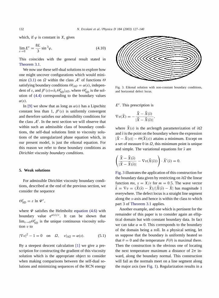
Fig. 3. Eikonal solution with non-constant boundary conditions,and horizontal defect locus.

Eε. This prescription is

∇v( X) = −X− X(s)

| X− X(s)| ,

where X(s) is the arclength parameterization of∂Ωands is the point on the boundary where the expression| X− X(s)| −Θ( X(s)) attains a minimum. Except ona set of measure 0 inΩ, this minimum point is uniqueand simple. The variational equations fors are( X− X(s)

| X− X(s)| − ∇v( X(s)))

· X′(s) = 0.

Fig. 3illustrates the application of this construction forthe boundary data given by restricting on∂Ω the linearfunction mx, x = X/ε for m = 0.5. The wave vectork = ∇v = ( X(s) − X)/| X(s) − X| has magnitude 1everywhere. The defect locus is a straight line segmentalong thex-axis and hence is within the class to whichpart 3 ofTheorem 3.1applies.

Another example, and one which is pertinent for theremainder of this paper is to consider again an ellip-tical domain but with constant boundary data. In factwe can takeα ≡ 0. This corresponds to the boundaryof the domain being a roll. In a physical setting, letus suppose that the boundary is uniformly heated sothatθ = 0 and the temperatureF(θ) is maximal there.Then the construction is the obvious one of locatingthe next temperature maximum a distance of 2π in-ward, along the boundary normal. This constructionwill fail as the normals meet on a line segment alongthe major axis (seeFig. 1). Regularization results in a


PGB along that segment; it is centered about the ori-gin between two points which are the curvature cen-ters of the ellipse and which we refer to as terminaldisclinations. Associated with each point on this opensegment there are two distinct points on the boundarywhich have the same distance to the given point onthe segment. Therefore forX on (or within a wave-length distance of) the line segment joining the twoterminal disclinations, from the steepest descent argu-ment,Ψ( X) is well approximated as the sum of twoexponentials

Ψ( X) ≈ exp

(1

εk1 · ( X− X(1)(s))

)

+exp

(1

εk2 · ( X− X(2)(s))

), (5.2)

where kj = ( X(j)(s) − X)/| X − X(j)(s)|, andX(j)(s), j = 1,2, are the two minimizing boundarypoints for X on the line segment joining the twoterminal disclinations. It is natural to regard this asa modulated PGB solution. This example will bediscussed in further detail inSection 8.

6. Multiple values and twist

Because the variational problem (3.1) studied in[1]considers only variations over fields which are con-servative, it cannot realize certain types of defects,such as disclinations, which are commonly seen inpattern-forming systems far from threshold. The rea-son is topological. Modulation equations such as CNor RCN are derived under the assumption that the fieldis locally gradient. Away from defects, striped patternslocally look like the level curves of a function such ascos(θ). The phaseθ itself need not be well defined (forinstance,θ → −θ leaves the local pattern unaltered).The existence of these ambiguities is intimately relatedto the types of defects that can occur. For instance,wave vector fields(f, g) with f − ig = z1/2 or z−1/2,wherez = x + iy give examples of harmonic vectorfields for which there is not asingle-valuedpotentialθ. Traversing a closed circuit counterclockwise aboutthe origin of these fields one would find that the wavevector returns to itself but rotated by∓π, in contrast

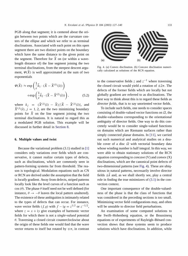
Fig. 4. (a) Convex disclination. (b) Concave disclination numeri-cally calculated as solutions of the RCN equation.

to the conservative fieldsz andz−1 where traversingthe closed circuit would yield a rotation of±2π. Thedefects of the former fields which are locally but notglobally gradient are referred to as disclinations. Thebest way to think about this is to regard these fields asdirector fields, that is to say unoriented vector fields.

To include such fields, one needs to consider spacesconsisting of double-valued vector functions onΩ, thedouble-valuedness corresponding to the orientationalambiguity of director fields. One way to do this con-cretely would be to consider single-valued functionson domains which are Riemann surfaces rather thansimply connected planar domains. In[11], we carriedout such numerical and analytical studies on a dou-ble cover of a discΩ with vectorial boundary datawhose winding number is half integral. In this way, wewere able to obtain stationary solutions of the RCNequation corresponding toconcave(V) andconvex(X)disclinations, which are the canonical point defects oftwo-dimensional patterns (seeFig. 4). These are ubiq-uitous in natural patterns, necessarily involve directorfields ±k and, as we shall shortly see, play a centralrole in finding the true minimizers of(3.1) in the con-vection context.

One important consequence of the double-valued-ness of the phase is that the class of functions thatwas considered in the preceding sections is too small.Minimizing vector field configurations may, and oftenwill be unstable to director field perturbations.

An examination of some computed solutions tothe Swift–Hohenberg equation, or the Boussinesqequations or of experiments of Rayleigh–Bénard con-vection shows that these systems seem to producesolutions which have disclinations. In addition, while


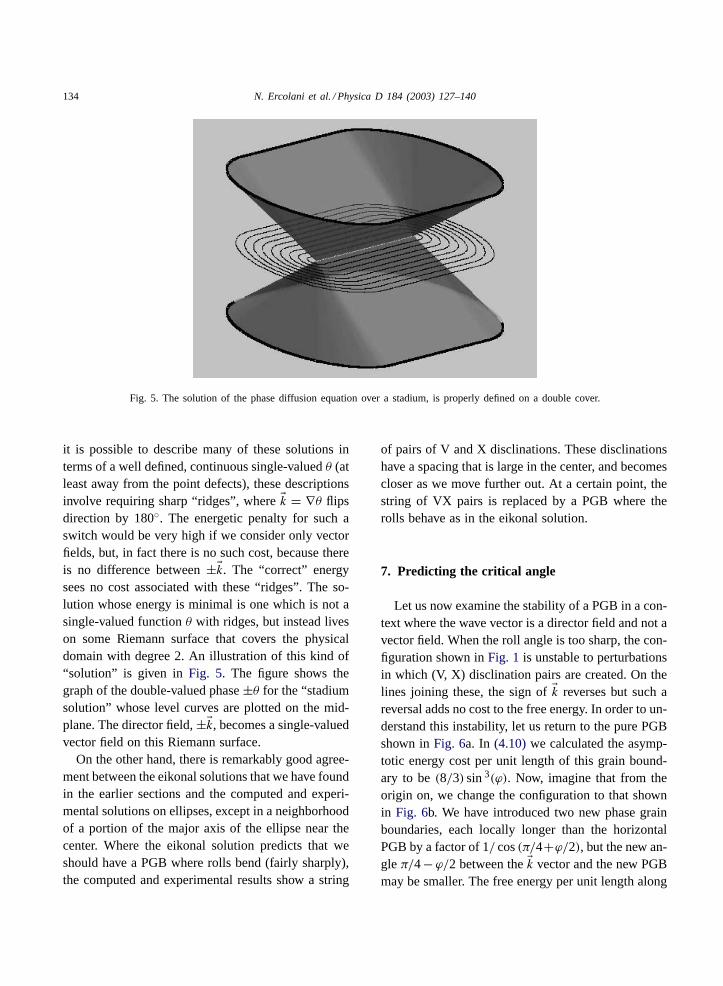
Fig. 5. The solution of the phase diffusion equation over a stadium, is properly defined on a double cover.

it is possible to describe many of these solutions interms of a well defined, continuous single-valuedθ (atleast away from the point defects), these descriptionsinvolve requiring sharp “ridges”, wherek = ∇θ flipsdirection by 180. The energetic penalty for such aswitch would be very high if we consider only vectorfields, but, in fact there is no such cost, because thereis no difference between±k. The “correct” energysees no cost associated with these “ridges”. The so-lution whose energy is minimal is one which is not asingle-valued functionθ with ridges, but instead liveson some Riemann surface that covers the physicaldomain with degree 2. An illustration of this kind of“solution” is given in Fig. 5. The figure shows thegraph of the double-valued phase±θ for the “stadiumsolution” whose level curves are plotted on the mid-plane. The director field,±k, becomes a single-valuedvector field on this Riemann surface.

On the other hand, there is remarkably good agree-ment between the eikonal solutions that we have foundin the earlier sections and the computed and experi-mental solutions on ellipses, except in a neighborhoodof a portion of the major axis of the ellipse near thecenter. Where the eikonal solution predicts that weshould have a PGB where rolls bend (fairly sharply),the computed and experimental results show a string

of pairs of V and X disclinations. These disclinationshave a spacing that is large in the center, and becomescloser as we move further out. At a certain point, thestring of VX pairs is replaced by a PGB where therolls behave as in the eikonal solution.

7. Predicting the critical angle

Let us now examine the stability of a PGB in a con-text where the wave vector is a director field and not avector field. When the roll angle is too sharp, the con-figuration shown inFig. 1 is unstable to perturbationsin which (V, X) disclination pairs are created. On thelines joining these, the sign ofk reverses but such areversal adds no cost to the free energy. In order to un-derstand this instability, let us return to the pure PGBshown inFig. 6a. In (4.10)we calculated the asymp-totic energy cost per unit length of this grain bound-ary to be(8/3) sin3(ϕ). Now, imagine that from theorigin on, we change the configuration to that shownin Fig. 6b. We have introduced two new phase grainboundaries, each locally longer than the horizontalPGB by a factor of 1/ cos(π/4+ϕ/2), but the new an-gleπ/4−ϕ/2 between thek vector and the new PGBmay be smaller. The free energy per unit length along


Fig. 6. (a) A single PGB may have higher energy than (b) a configuration of three phase grain boundaries with a pair of disclinations(phase grain boundaries are shown as thin solid gray lines).

the pair of phase grain boundaries shown inFig. 6b is

2

cos(π/4 + ϕ/2) sin3(π

4− ϕ

2

) 8

3

= 8

3(1 − sinϕ). (7.1)

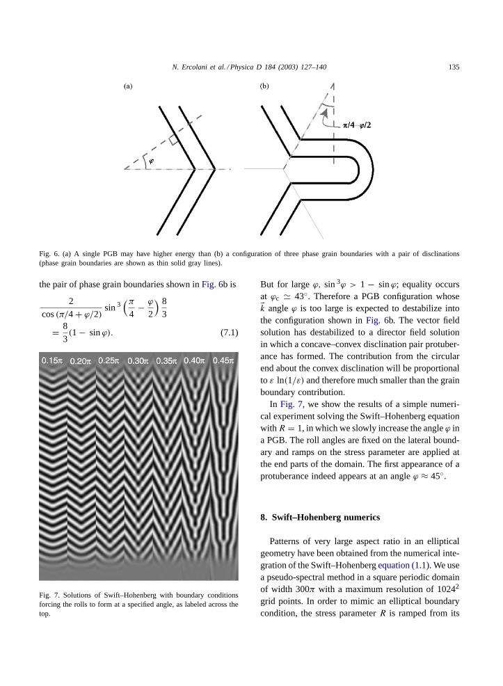
Fig. 7. Solutions of Swift–Hohenberg with boundary conditionsforcing the rolls to form at a specified angle, as labeled across thetop.

But for largeϕ, sin3ϕ > 1 − sinϕ; equality occursat ϕc 43. Therefore a PGB configuration whosek angleϕ is too large is expected to destabilize intothe configuration shown inFig. 6b. The vector fieldsolution has destabilized to a director field solutionin which a concave–convex disclination pair protuber-ance has formed. The contribution from the circularend about the convex disclination will be proportionalto ε ln(1/ε) and therefore much smaller than the grainboundary contribution.

In Fig. 7, we show the results of a simple numeri-cal experiment solving the Swift–Hohenberg equationwithR = 1, in which we slowly increase the angleϕ ina PGB. The roll angles are fixed on the lateral bound-ary and ramps on the stress parameter are applied atthe end parts of the domain. The first appearance of aprotuberance indeed appears at an angleϕ ≈ 45.

8. Swift–Hohenberg numerics

Patterns of very large aspect ratio in an ellipticalgeometry have been obtained from the numerical inte-gration of the Swift–Hohenbergequation (1.1). We usea pseudo-spectral method in a square periodic domainof width 300π with a maximum resolution of 10242

grid points. In order to mimic an elliptical boundarycondition, the stress parameterR is ramped from its


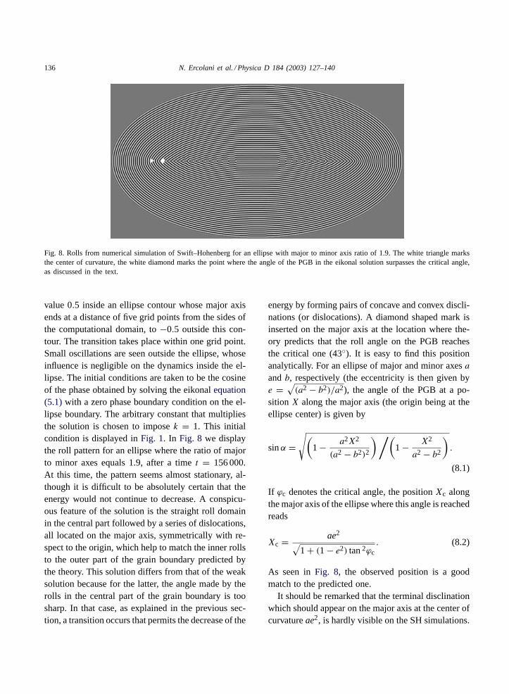
Fig. 8. Rolls from numerical simulation of Swift–Hohenberg for an ellipse with major to minor axis ratio of 1.9. The white triangle marksthe center of curvature, the white diamond marks the point where the angle of the PGB in the eikonal solution surpasses the critical angle,as discussed in the text.

value 0.5 inside an ellipse contour whose major axisends at a distance of five grid points from the sides ofthe computational domain, to−0.5 outside this con-tour. The transition takes place within one grid point.Small oscillations are seen outside the ellipse, whoseinfluence is negligible on the dynamics inside the el-lipse. The initial conditions are taken to be the cosineof the phase obtained by solving the eikonalequation(5.1) with a zero phase boundary condition on the el-lipse boundary. The arbitrary constant that multipliesthe solution is chosen to imposek = 1. This initialcondition is displayed inFig. 1. In Fig. 8 we displaythe roll pattern for an ellipse where the ratio of majorto minor axes equals 1.9, after a timet = 156 000.At this time, the pattern seems almost stationary, al-though it is difficult to be absolutely certain that theenergy would not continue to decrease. A conspicu-ous feature of the solution is the straight roll domainin the central part followed by a series of dislocations,all located on the major axis, symmetrically with re-spect to the origin, which help to match the inner rollsto the outer part of the grain boundary predicted bythe theory. This solution differs from that of the weaksolution because for the latter, the angle made by therolls in the central part of the grain boundary is toosharp. In that case, as explained in the previous sec-tion, a transition occurs that permits the decrease of the

energy by forming pairs of concave and convex discli-nations (or dislocations). A diamond shaped mark isinserted on the major axis at the location where the-ory predicts that the roll angle on the PGB reachesthe critical one (43). It is easy to find this positionanalytically. For an ellipse of major and minor axesaandb, respectively (the eccentricity is then given bye =

√(a2 − b2)/a2), the angle of the PGB at a po-

sitionX along the major axis (the origin being at theellipse center) is given by

sinα =√(

1 − a2X2

(a2 − b2)2

)/(1 − X2

a2 − b2

).

(8.1)

If ϕc denotes the critical angle, the positionXc alongthe major axis of the ellipse where this angle is reachedreads

Xc = ae2√1 + (1 − e2) tan2ϕc

. (8.2)

As seen inFig. 8, the observed position is a goodmatch to the predicted one.

It should be remarked that the terminal disclinationwhich should appear on the major axis at the center ofcurvatureae2, is hardly visible on the SH simulations.


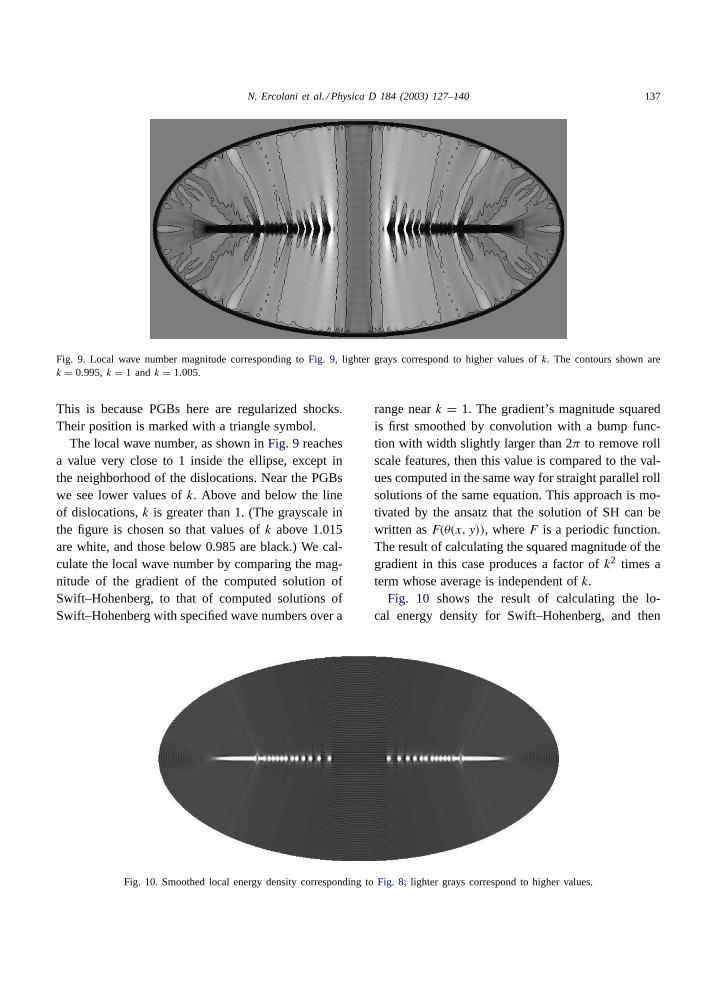
Fig. 9. Local wave number magnitude corresponding toFig. 9, lighter grays correspond to higher values ofk. The contours shown arek = 0.995, k = 1 andk = 1.005.

This is because PGBs here are regularized shocks.Their position is marked with a triangle symbol.

The local wave number, as shown inFig. 9 reachesa value very close to 1 inside the ellipse, except inthe neighborhood of the dislocations. Near the PGBswe see lower values ofk. Above and below the lineof dislocations,k is greater than 1. (The grayscale inthe figure is chosen so that values ofk above 1.015are white, and those below 0.985 are black.) We cal-culate the local wave number by comparing the mag-nitude of the gradient of the computed solution ofSwift–Hohenberg, to that of computed solutions ofSwift–Hohenberg with specified wave numbers over a

Fig. 10. Smoothed local energy density corresponding toFig. 8; lighter grays correspond to higher values.

range neark = 1. The gradient’s magnitude squaredis first smoothed by convolution with a bump func-tion with width slightly larger than 2π to remove rollscale features, then this value is compared to the val-ues computed in the same way for straight parallel rollsolutions of the same equation. This approach is mo-tivated by the ansatz that the solution of SH can bewritten asF(θ(x, y)), whereF is a periodic function.The result of calculating the squared magnitude of thegradient in this case produces a factor ofk2 times aterm whose average is independent ofk.

Fig. 10 shows the result of calculating the lo-cal energy density for Swift–Hohenberg, and then


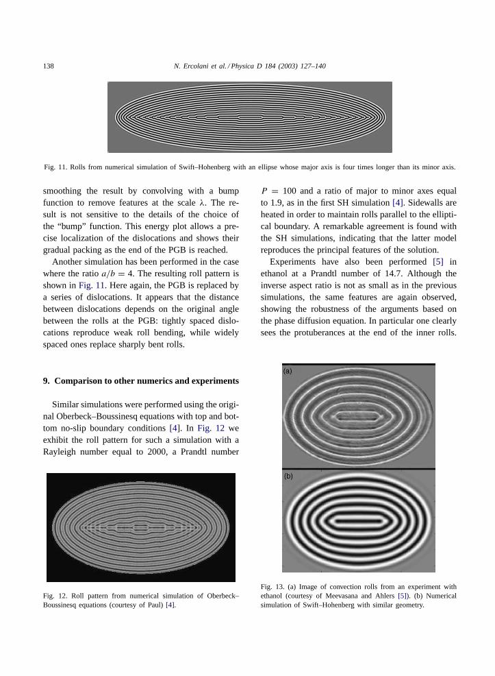
Fig. 11. Rolls from numerical simulation of Swift–Hohenberg with an ellipse whose major axis is four times longer than its minor axis.

smoothing the result by convolving with a bumpfunction to remove features at the scaleλ. The re-sult is not sensitive to the details of the choice ofthe “bump” function. This energy plot allows a pre-cise localization of the dislocations and shows theirgradual packing as the end of the PGB is reached.

Another simulation has been performed in the casewhere the ratioa/b = 4. The resulting roll pattern isshown inFig. 11. Here again, the PGB is replaced bya series of dislocations. It appears that the distancebetween dislocations depends on the original anglebetween the rolls at the PGB: tightly spaced dislo-cations reproduce weak roll bending, while widelyspaced ones replace sharply bent rolls.

9. Comparison to other numerics and experiments

Similar simulations were performed using the origi-nal Oberbeck–Boussinesq equations with top and bot-tom no-slip boundary conditions[4]. In Fig. 12 weexhibit the roll pattern for such a simulation with aRayleigh number equal to 2000, a Prandtl number

Fig. 12. Roll pattern from numerical simulation of Oberbeck–Boussinesq equations (courtesy of Paul)[4].

P = 100 and a ratio of major to minor axes equalto 1.9, as in the first SH simulation[4]. Sidewalls areheated in order to maintain rolls parallel to the ellipti-cal boundary. A remarkable agreement is found withthe SH simulations, indicating that the latter modelreproduces the principal features of the solution.

Experiments have also been performed[5] inethanol at a Prandtl number of 14.7. Although theinverse aspect ratio is not as small as in the previoussimulations, the same features are again observed,showing the robustness of the arguments based onthe phase diffusion equation. In particular one clearlysees the protuberances at the end of the inner rolls.

Fig. 13. (a) Image of convection rolls from an experiment withethanol (courtesy of Meevasana and Ahlers[5]). (b) Numericalsimulation of Swift–Hohenberg with similar geometry.


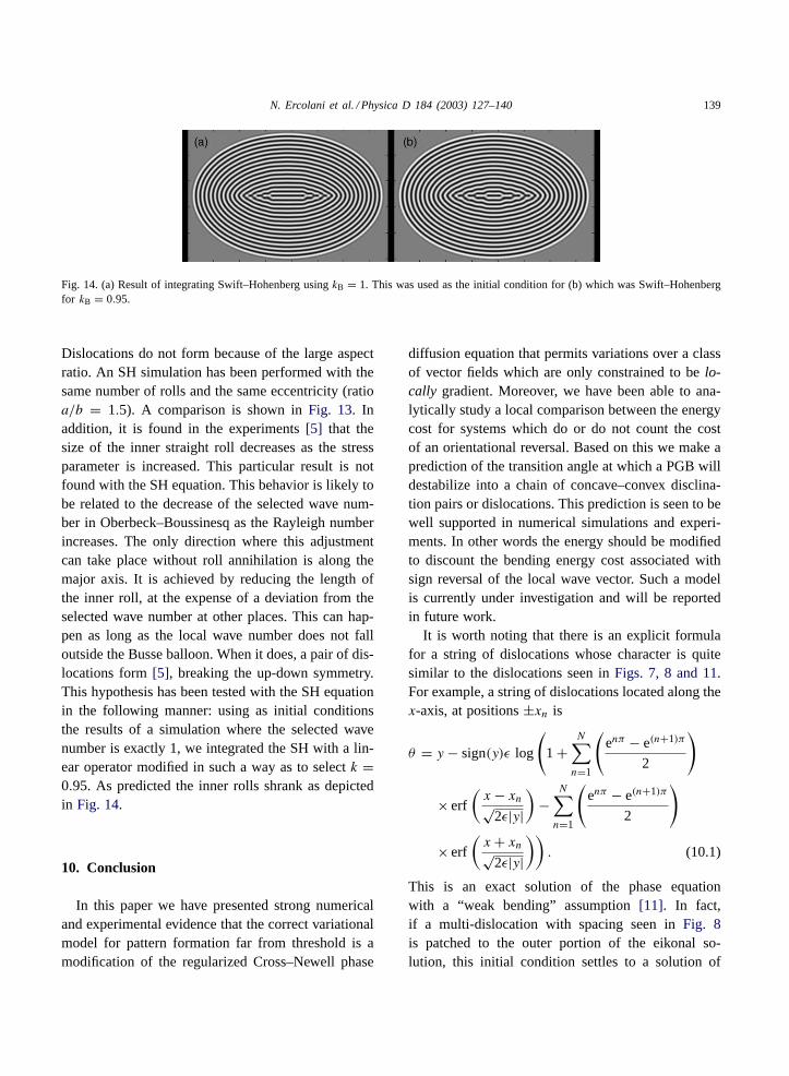
Fig. 14. (a) Result of integrating Swift–Hohenberg usingkB = 1. This was used as the initial condition for (b) which was Swift–Hohenbergfor kB = 0.95.

Dislocations do not form because of the large aspectratio. An SH simulation has been performed with thesame number of rolls and the same eccentricity (ratioa/b = 1.5). A comparison is shown inFig. 13. Inaddition, it is found in the experiments[5] that thesize of the inner straight roll decreases as the stressparameter is increased. This particular result is notfound with the SH equation. This behavior is likely tobe related to the decrease of the selected wave num-ber in Oberbeck–Boussinesq as the Rayleigh numberincreases. The only direction where this adjustmentcan take place without roll annihilation is along themajor axis. It is achieved by reducing the length ofthe inner roll, at the expense of a deviation from theselected wave number at other places. This can hap-pen as long as the local wave number does not falloutside the Busse balloon. When it does, a pair of dis-locations form[5], breaking the up-down symmetry.This hypothesis has been tested with the SH equationin the following manner: using as initial conditionsthe results of a simulation where the selected wavenumber is exactly 1, we integrated the SH with a lin-ear operator modified in such a way as to selectk =0.95. As predicted the inner rolls shrank as depictedin Fig. 14.

10. Conclusion

In this paper we have presented strong numericaland experimental evidence that the correct variationalmodel for pattern formation far from threshold is amodification of the regularized Cross–Newell phase

diffusion equation that permits variations over a classof vector fields which are only constrained to belo-cally gradient. Moreover, we have been able to ana-lytically study a local comparison between the energycost for systems which do or do not count the costof an orientational reversal. Based on this we make aprediction of the transition angle at which a PGB willdestabilize into a chain of concave–convex disclina-tion pairs or dislocations. This prediction is seen to bewell supported in numerical simulations and experi-ments. In other words the energy should be modifiedto discount the bending energy cost associated withsign reversal of the local wave vector. Such a modelis currently under investigation and will be reportedin future work.

It is worth noting that there is an explicit formulafor a string of dislocations whose character is quitesimilar to the dislocations seen inFigs. 7, 8 and 11.For example, a string of dislocations located along thex-axis, at positions±xn is

θ = y − sign(y)ε log

(1 +

N∑n=1

(enπ − e(n+1)π

2

)

× erf

(x− xn√

2ε|y|)

−N∑n=1

(enπ − e(n+1)π

2

)

× erf

(x+ xn√

2ε|y|)). (10.1)

This is an exact solution of the phase equationwith a “weak bending” assumption[11]. In fact,if a multi-dislocation with spacing seen inFig. 8is patched to the outer portion of the eikonal so-lution, this initial condition settles to a solution of


the same form with the position of the dislocationsessentially unchanged. (The only real changes arealong the interface where the solutions are patchedtogether.)

Another natural extension of the RCN problem isto study minimizers of the free energy

F=∫Ω

(|∇k|2 + 1

ε2(k2 − 1)2 + 1

µ2(∇ × k)2

)dX(10.2)

in the limitsε, µ→ 0. We note that the case whereε isset to infinity and only limits inµ are considered cor-responds to a natural model[13] for micro-magneticsystems whose asymptotic minimizers are identical tothose described in[1]. Such a study may also haveimplications for models of defects in superconductors[14] and nematic liquid crystals[15].

Acknowledgements

The authors wish to thank Joceline Lega for manyhelpful discussions and in particular for generatingFig. 3. The authors also wish to thank Guenter Ahlersand Mark Paul for helpful discussion and for gen-erosity in sharing their results. NME would like toacknowledge support from NSF grant DMS-0073087and ACN would like to acknowledge support fromNSF grant DMS-0072803.

References

[1] N.M. Ercolani, R. Indik, A.C. Newell, T. Passot, Thegeometry of the phase diffusion equation, J. Nonlinear Sci.10 (2000) 223–274.

[2] M.C. Cross, P.C. Hohenberg, Pattern formation outside ofequilibrium, Rev. Mod. Phys. 65 (1993) 851–1112.

[3] Y. Pomeau, Caustics of nonlinear waves and related questions,Europhys. Lett. 11 (1990) 713–718.

[4] M. Paul, Private communication.[5] W. Meevasana, G. Ahlers, Private communication.[6] F.H. Busse, On the stability of two-dimensional convection in

a layer heated from below, J. Math. Phys. 46 (1967) 149–150.[7] M.C. Cross, A.C. Newell, Convection patterns in large aspect

ratio systems, Physica D 10 (1984) 299–328.[8] L. Ambrosio, C. DeLellis, C. Mantegazza, Line energies for

gradient vector fields in the plane, Calc. Var. 9 (1999) 327–355.

[9] N.M. Ercolani, M. Taylor, The Dirichlet-to-Neumann map,viscosity solutions to eikonal equations, and the self-dualequations of pattern formation, Preprint, 2002.

[10] A. DeSimone, R.V. Kohn, S. Muller, F. Otto, A compactnessresult in the gradient theory of phase transitions, Proc. R.Soc. Edinburgh Sect. A 131 (2001) 833–844.

[11] A.C. Newell, T. Passot, C. Bowman, N.M. Ercolani, R. Indik,Defects are weak and self-dual solutions of the Cross–Newellphase diffusion equation for natural patterns, Physica D 97(1996) 185–205.

[12] T. Passot, A.C. Newell, Towards a universal theory of patterns,Physica D 74 (1994) 301–352.

[13] W. Jin, R. Kohn, Singular perturbation and the energy offolds, J. Nonlinear Sci. 10 (2000) 355–390.

[14] A. Jaffe, C. Taubes, Vortices and Monopoles, Birkhauser,Boston, 1980.

[15] F.H. Lin, Nonlinear theory of defects in nematic liquidcrystals; phase transition and flow phenomena, Commun. PureAppl. Math. 42 (1989) 789–914.

Global description of patterns far from onset: a case...

Documents

Transcript of Global description of patterns far from onset: a case...