Gaussian Mixtures and the EM Algorithmrtc12/CSE586/lectures/EMLectureFeb3.pdfCSE586 Robert Collins...
43
CSE586 Robert Collins Gaussian Mixtures and the EM Algorithm Reading: Chapter 7.4, Prince book
Transcript of Gaussian Mixtures and the EM Algorithmrtc12/CSE586/lectures/EMLectureFeb3.pdfCSE586 Robert Collins...

CSE586
Robert Collins
Gaussian Mixtures and the EM Algorithm
Reading: Chapter 7.4, Prince book
Review: The Gaussian Distribu3on • Mul3variate Gaussian
mean covariance
Bishop, 2003
Isotropic (spherical) if covariance is diag(σ2, σ2,..., σ2)
dx1 vector dxd matrix
Evaluates to a number
d (( 2π )
CSE586
Robert Collins
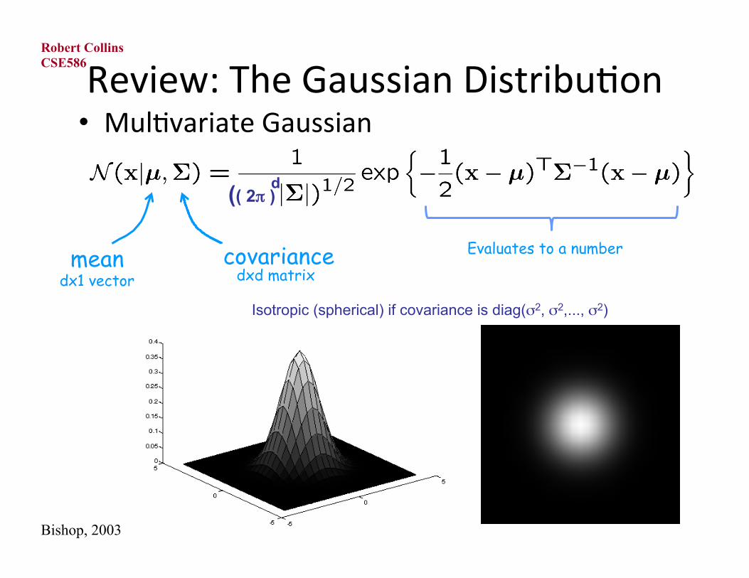
Likelihood Func3on • Data set
• Assume observed data points generated independently
• Viewed as a func3on of the parameters, this is known as the likelihood func-on
Bishop, 2003
CSE586
Robert Collins
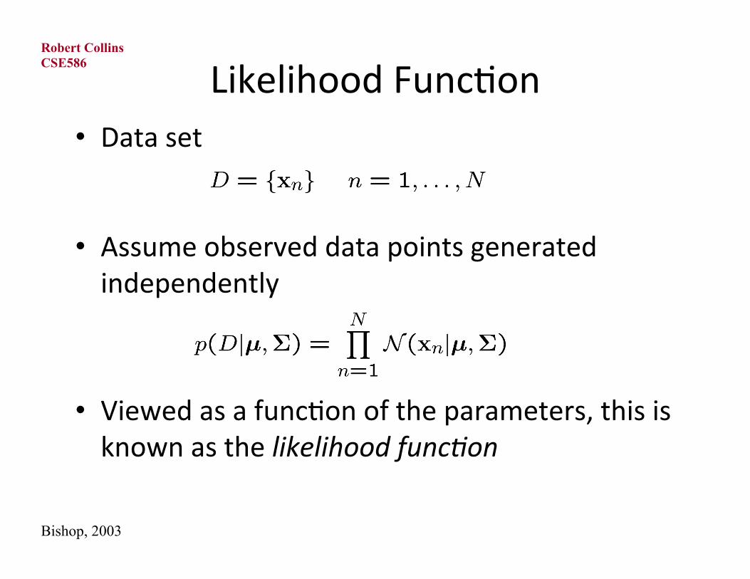
Maximum Likelihood • Set the parameters by maximizing the likelihood func3on
• Equivalently maximize the log likelihood
Bishop, 2003
d
CSE586
Robert Collins
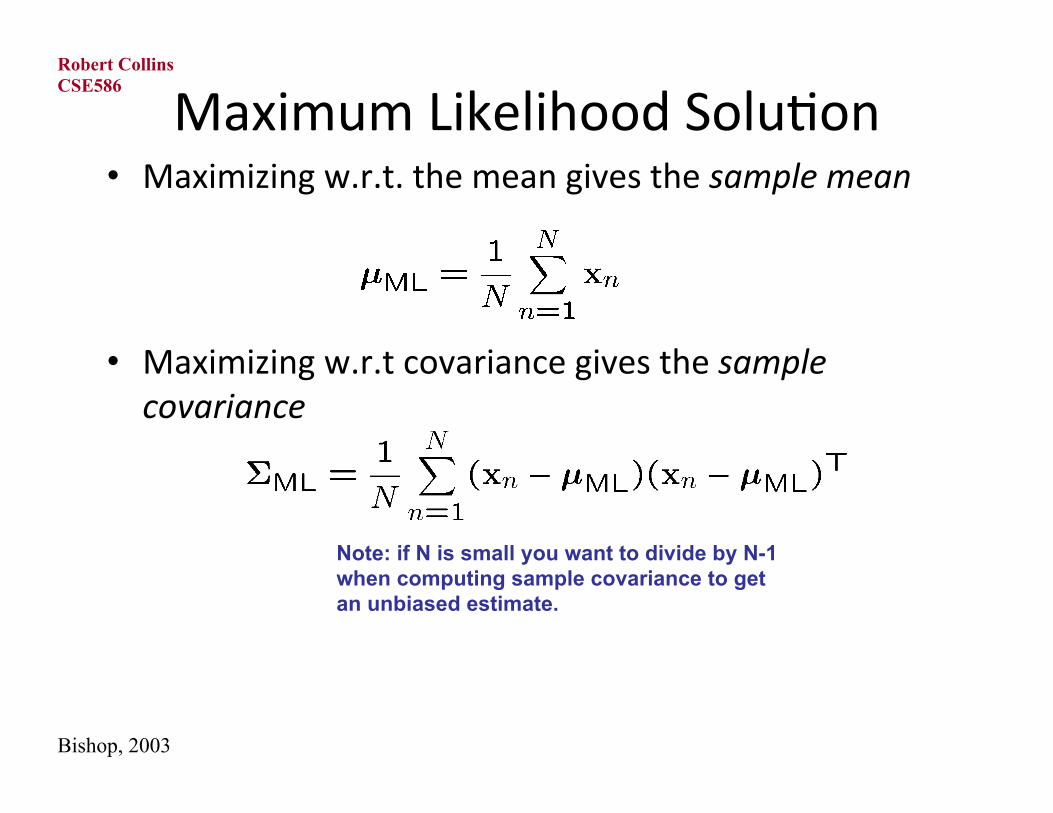
Maximum Likelihood Solu3on • Maximizing w.r.t. the mean gives the sample mean
• Maximizing w.r.t covariance gives the sample covariance
Bishop, 2003
Note: if N is small you want to divide by N-1 when computing sample covariance to get an unbiased estimate.
CSE586
Robert Collins
Comments
Gaussians are well understood and easy to estimate However, they are unimodal, thus cannot be used to represent inherently multimodal datasets Fitting a single Gaussian to a multimodal dataset is likely to give a mean value in an area with low probability, and to overestimate the covariance.
CSE586
Robert Collins
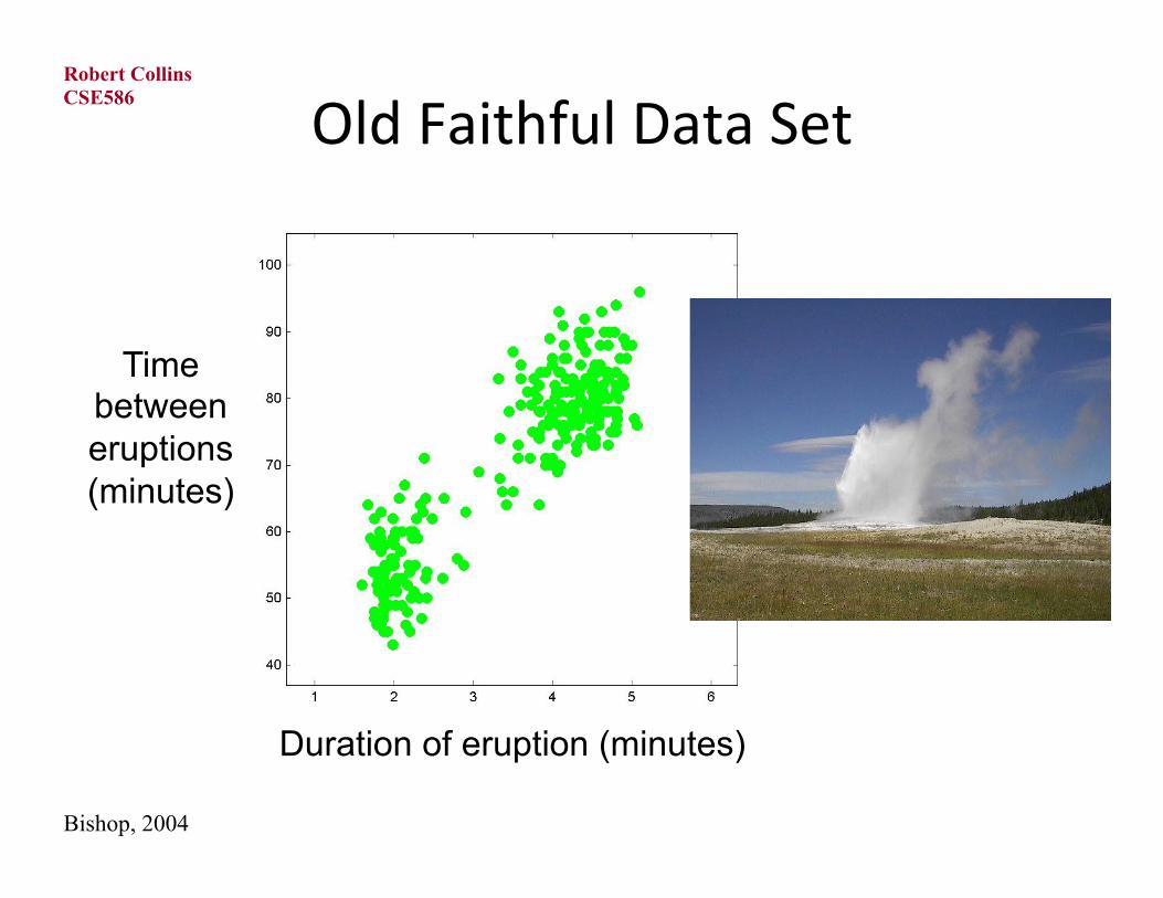
Old Faithful Data Set
Duration of eruption (minutes)
Time between eruptions (minutes)
Bishop, 2004
CSE586
Robert Collins

Idea: Use a Mixture of Gaussians • Convex Combina3on of Distribu3ons
• Normaliza3on and posi3vity require
• Can interpret the mixing coefficients as prior probabili3es
Bishop, 2003
CSE586
Robert Collins
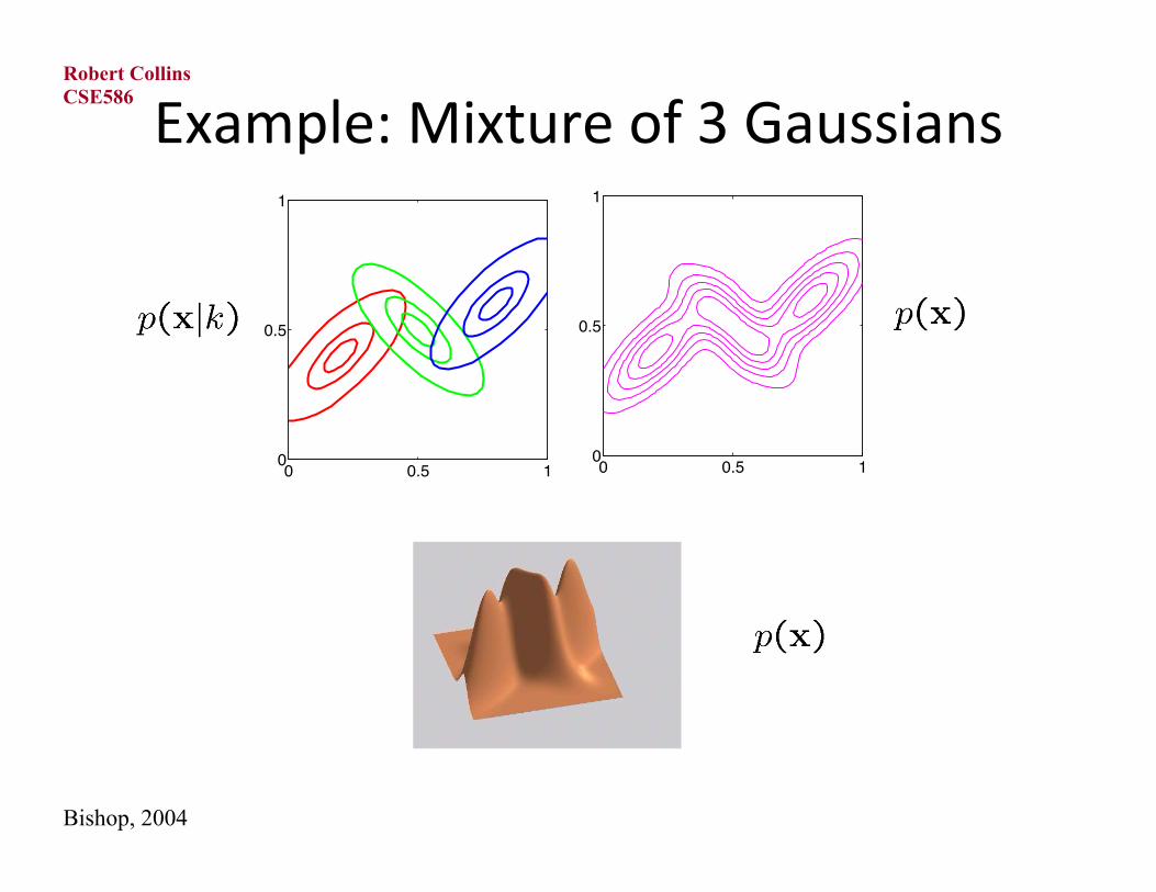
Example: Mixture of 3 Gaussians
0 0.5 10
0.5
1
(a)0 0.5 10
0.5
1
(b)
Bishop, 2004
CSE586
Robert Collins
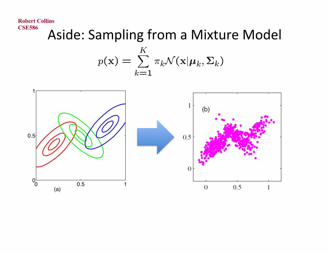
Aside: Sampling from a Mixture Model CSE586
Robert Collins
0 0.5 10
0.5
1
(a)
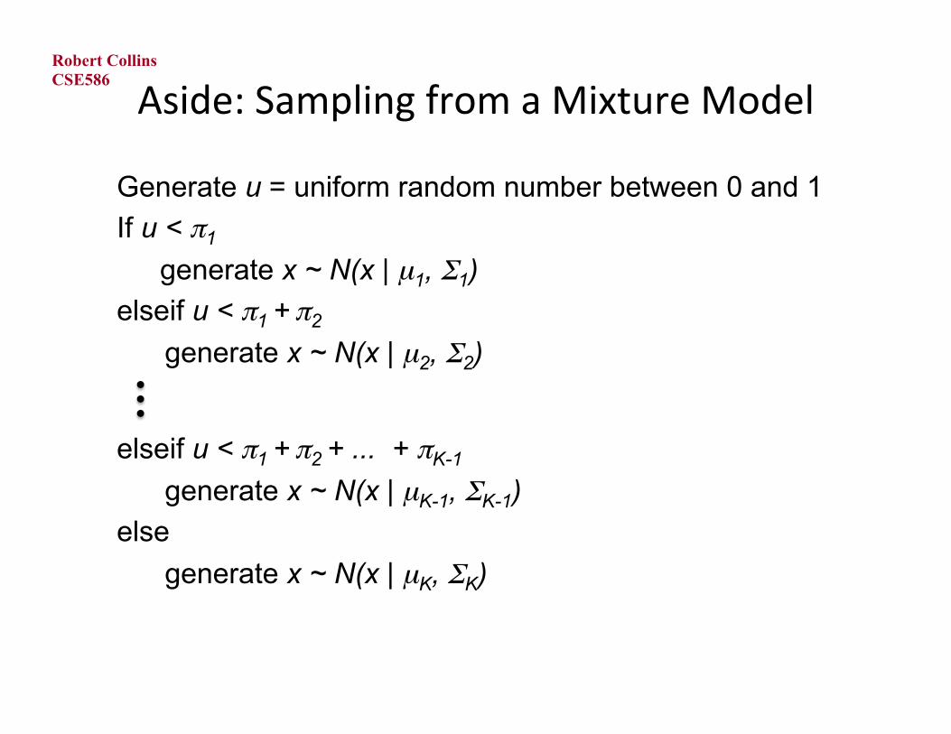
Aside: Sampling from a Mixture Model CSE586
Robert Collins
Generate u = uniform random number between 0 and 1 If u < π1
generate x ~ N(x | µ1, Σ1)
elseif u < π1 + π2
generate x ~ N(x | µ2, Σ2)
elseif u < π1 + π2 + ... + πK-1 generate x ~ N(x | µK-1, ΣK-1)
else generate x ~ N(x | µK, ΣK)
CSE586
Robert Collins
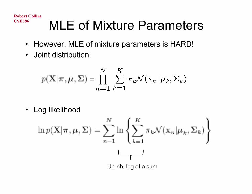
MLE of Mixture Parameters • However, MLE of mixture parameters is HARD! • Joint distribution:
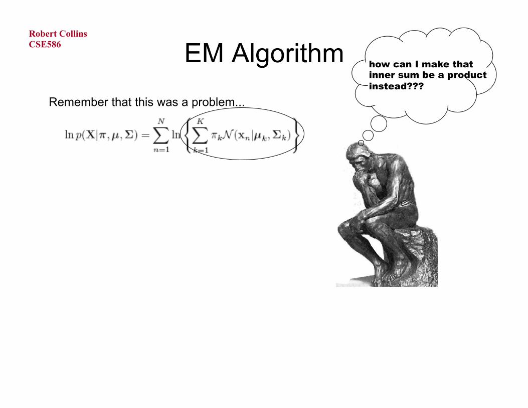
• Log likelihood
n
Uh-oh, log of a sum

CSE586
Robert Collins
EM Algorithm
What makes this estimation problem hard? 1) It is a mixture, so log-likelihood is messy 2) We don’t directly see what the underlying process is
CSE586
Robert Collins
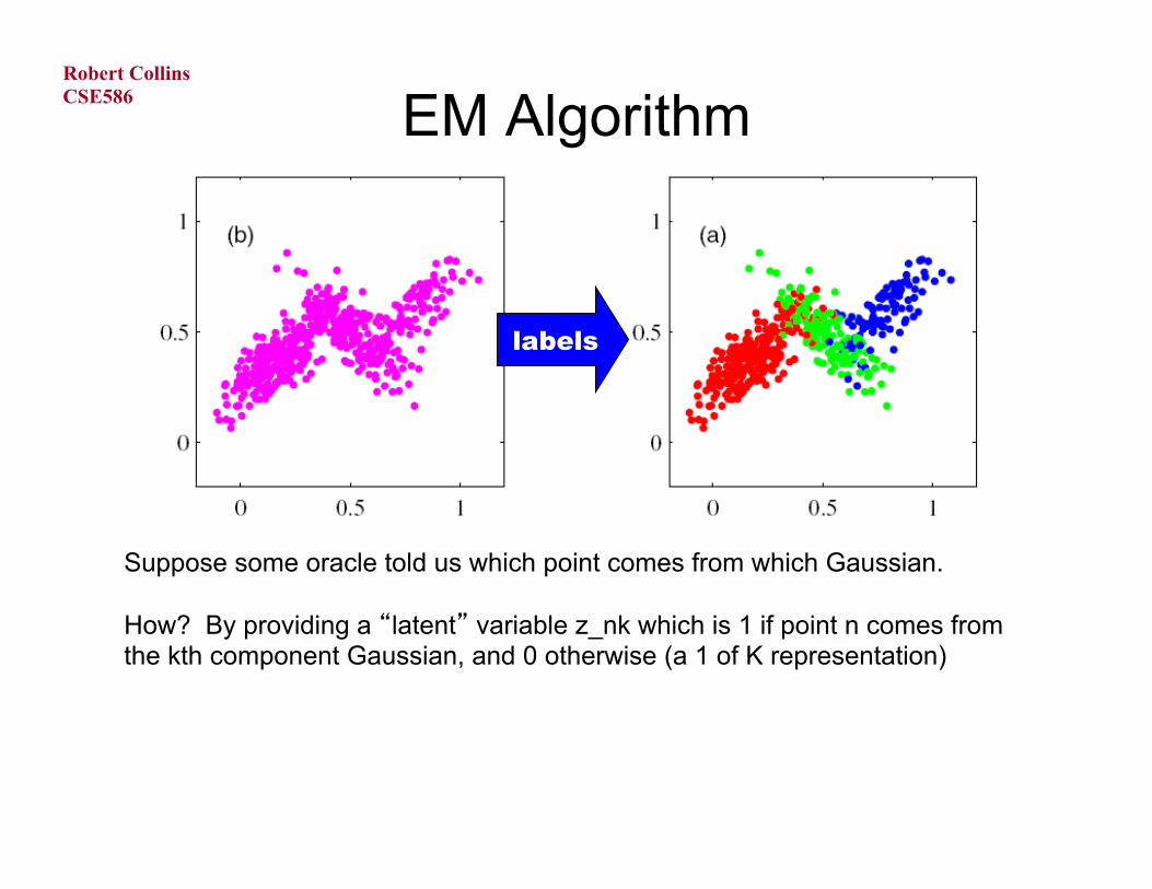
EM Algorithm
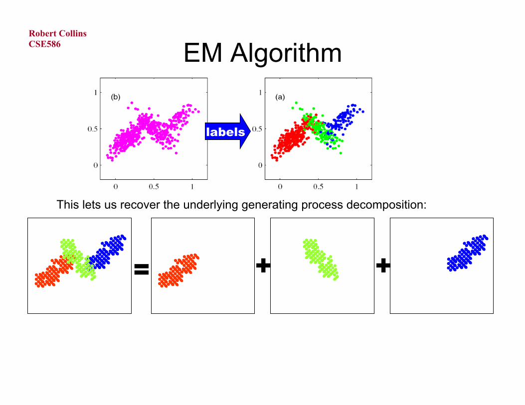
Suppose some oracle told us which point comes from which Gaussian. How? By providing a “latent” variable z_nk which is 1 if point n comes from the kth component Gaussian, and 0 otherwise (a 1 of K representation)
labels
CSE586
Robert Collins
EM Algorithm
This lets us recover the underlying generating process decomposition:
labels
+ + =
CSE586
Robert Collins
EM Algorithm
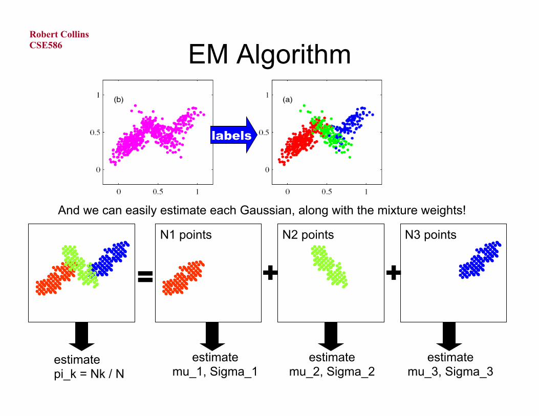
And we can easily estimate each Gaussian, along with the mixture weights!
labels
+ + =
estimate mu_1, Sigma_1
estimate mu_2, Sigma_2
estimate mu_3, Sigma_3
N1 points N2 points N3 points
estimate pi_k = Nk / N
CSE586
Robert Collins
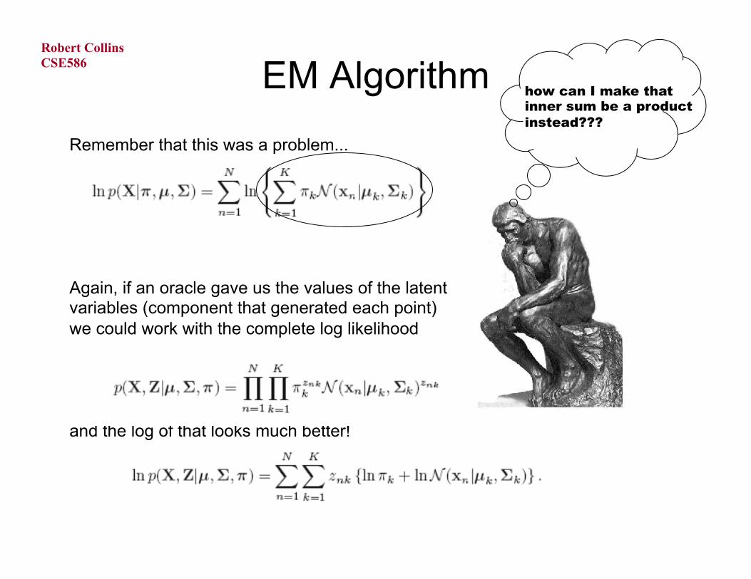
EM Algorithm Remember that this was a problem...
how can I make that inner sum be a product instead???
CSE586
Robert Collins
EM Algorithm Remember that this was a problem... Again, if an oracle gave us the values of the latent variables (component that generated each point) we could work with the complete log likelihood and the log of that looks much better!
how can I make that inner sum be a product instead???
CSE586
Robert Collins
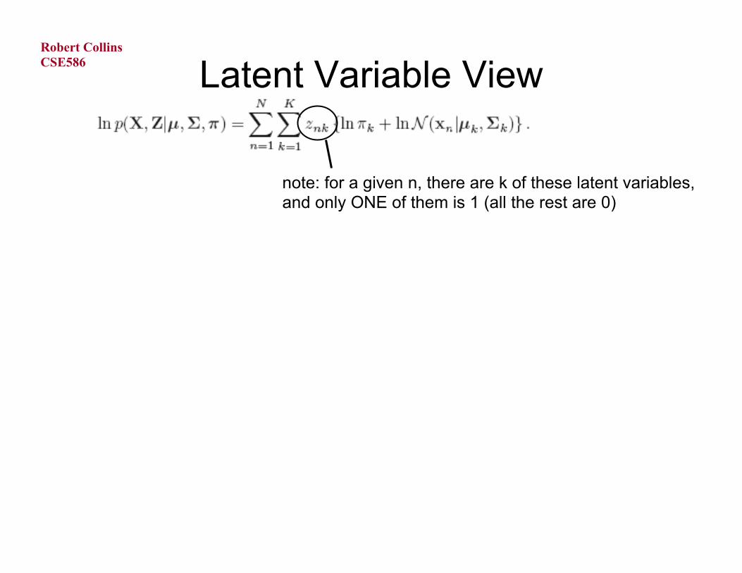
Latent Variable View
note: for a given n, there are k of these latent variables, and only ONE of them is 1 (all the rest are 0)
CSE586
Robert Collins
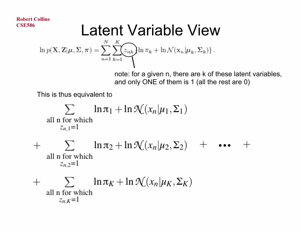
Latent Variable View
note: for a given n, there are k of these latent variables, and only ONE of them is 1 (all the rest are 0)
This is thus equivalent to

CSE586
Robert Collins
Latent Variable View
CSE586
Robert Collins
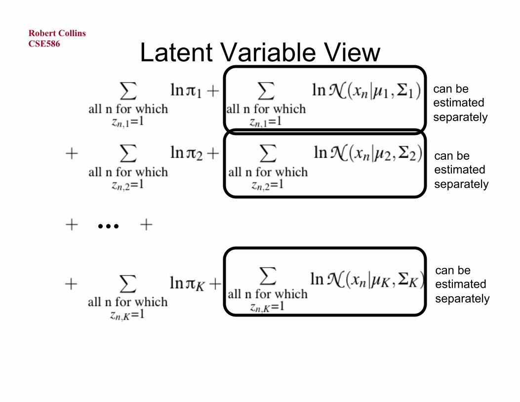
Latent Variable View can be estimated separately
can be estimated separately
can be estimated separately
CSE586
Robert Collins
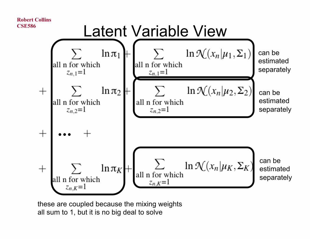
Latent Variable View can be estimated separately
can be estimated separately
can be estimated separately
these are coupled because the mixing weights all sum to 1, but it is no big deal to solve

CSE586
Robert Collins
EM Algorithm Unfortunately, oracles don’t exist (or if they do, they won’t talk to us) So we don’t know values of the the z_nk variables What EM proposes to do: 1) compute p(Z|X,theta), the posterior distribution over z_nk,
given our current best guess at the values of theta
2) compute the expected value of the log likelihood ln(p(X,Z|theta)) with respect to the distribution p(Z|X,theta)
3) find theta_new that maximizes that function. This is our new best guess at the values of theta.
4) iterate...
CSE586
Robert Collins
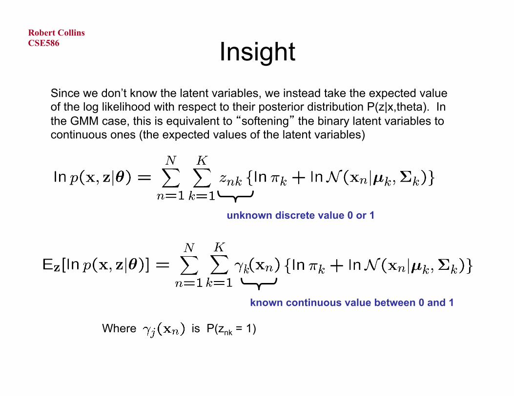
Insight
unknown discrete value 0 or 1
known continuous value between 0 and 1
Since we don’t know the latent variables, we instead take the expected value of the log likelihood with respect to their posterior distribution P(z|x,theta). In the GMM case, this is equivalent to “softening” the binary latent variables to continuous ones (the expected values of the latent variables)
Where is P(znk = 1)
CSE586
Robert Collins
Insight So now, after replacing the binary latent variables with their continuous expected values: all points contribute to the estimation of all components each point has unit mass to contribute, but splits it across the K components the amount of weight a point contributes to a component is proportional to the relative likelihood that the point was generated by that component

CSE586
Robert Collins
Latent Variable View (with an oracle) can be estimated separately
can be estimated separately
can be estimated separately
these are coupled because the mixing weights all sum to 1, but it is no big deal to solve
CSE586
Robert Collins
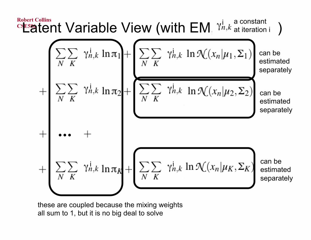
Latent Variable View (with EM, ) can be estimated separately
can be estimated separately
can be estimated separately
these are coupled because the mixing weights all sum to 1, but it is no big deal to solve
i
i
i
i
i
i
i a constant at iteration i
CSE586
Robert Collins
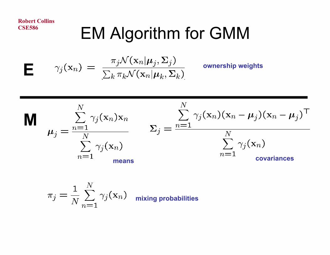
EM Algorithm for GMM
ownership weights
means covariances
mixing probabilities
E
M
CSE586
Robert Collins
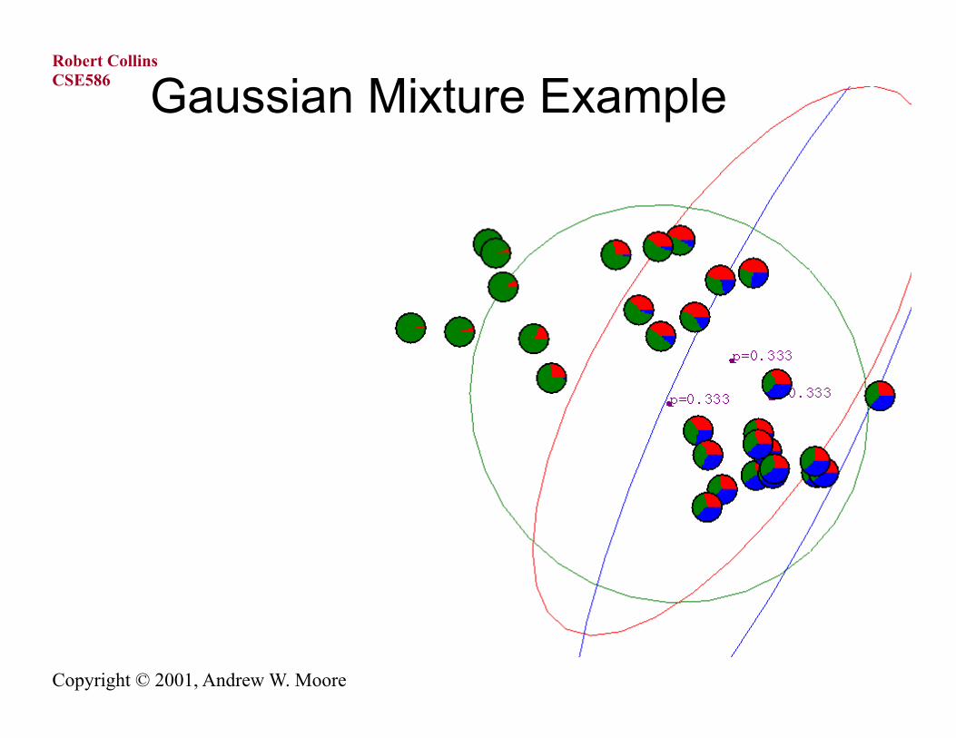
Copyright © 2001, Andrew W. Moore
Gaussian Mixture Example
CSE586
Robert Collins
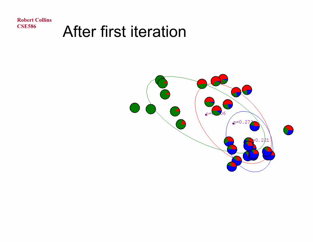
After first iteration

CSE586
Robert Collins
After 2nd iteration

CSE586
Robert Collins
After 3rd iteration

CSE586
Robert Collins
After 4th iteration

CSE586
Robert Collins
After 5th iteration
CSE586
Robert Collins
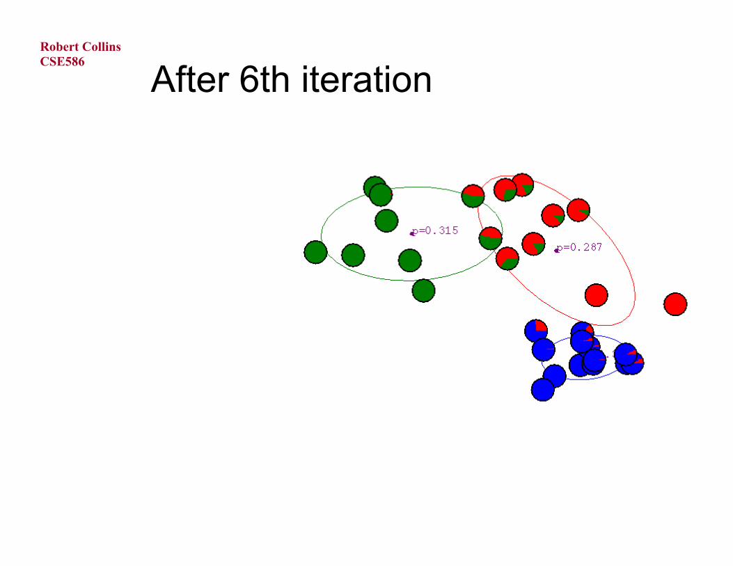
After 6th iteration
CSE586
Robert Collins
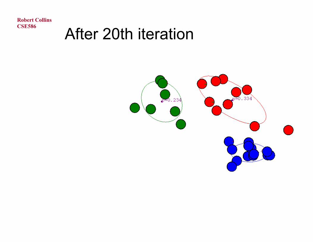
After 20th iteration
CSE586
Robert Collins
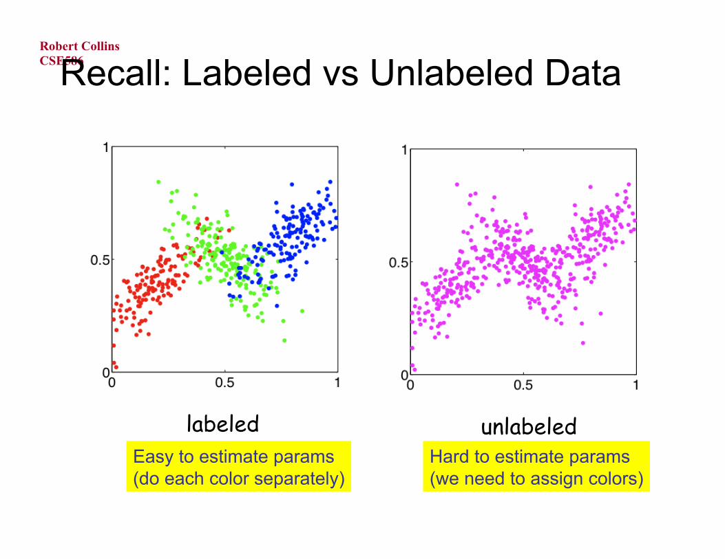
Recall: Labeled vs Unlabeled Data
labeled unlabeled Easy to estimate params (do each color separately)
Hard to estimate params (we need to assign colors)
CSE586
Robert Collins
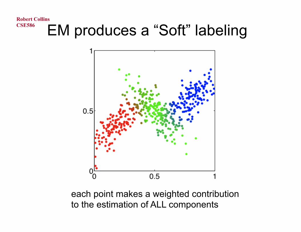
EM produces a “Soft” labeling
each point makes a weighted contribution to the estimation of ALL components
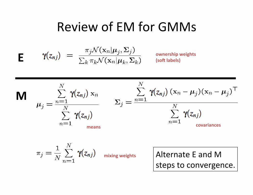
Review of EM for GMMs
ownership weights (so. labels)
means covariances
mixing weights
E
M
Alternate E and M steps to convergence.
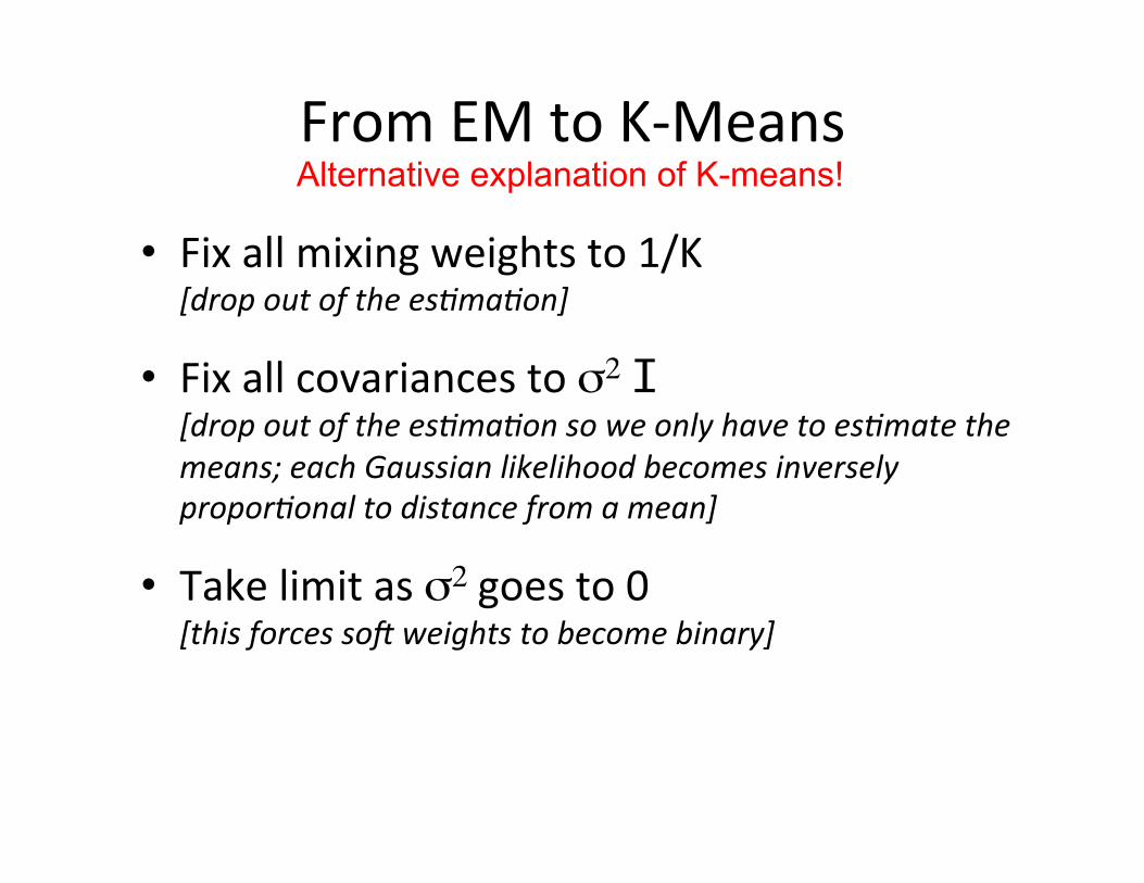
From EM to K-‐Means
• Fix all mixing weights to 1/K [drop out of the es-ma-on]
• Fix all covariances to σ2 I [drop out of the es-ma-on so we only have to es-mate the means; each Gaussian likelihood becomes inversely propor-onal to distance from a mean]
• Take limit as σ2 goes to 0 [this forces so< weights to become binary]
Alternative explanation of K-means!
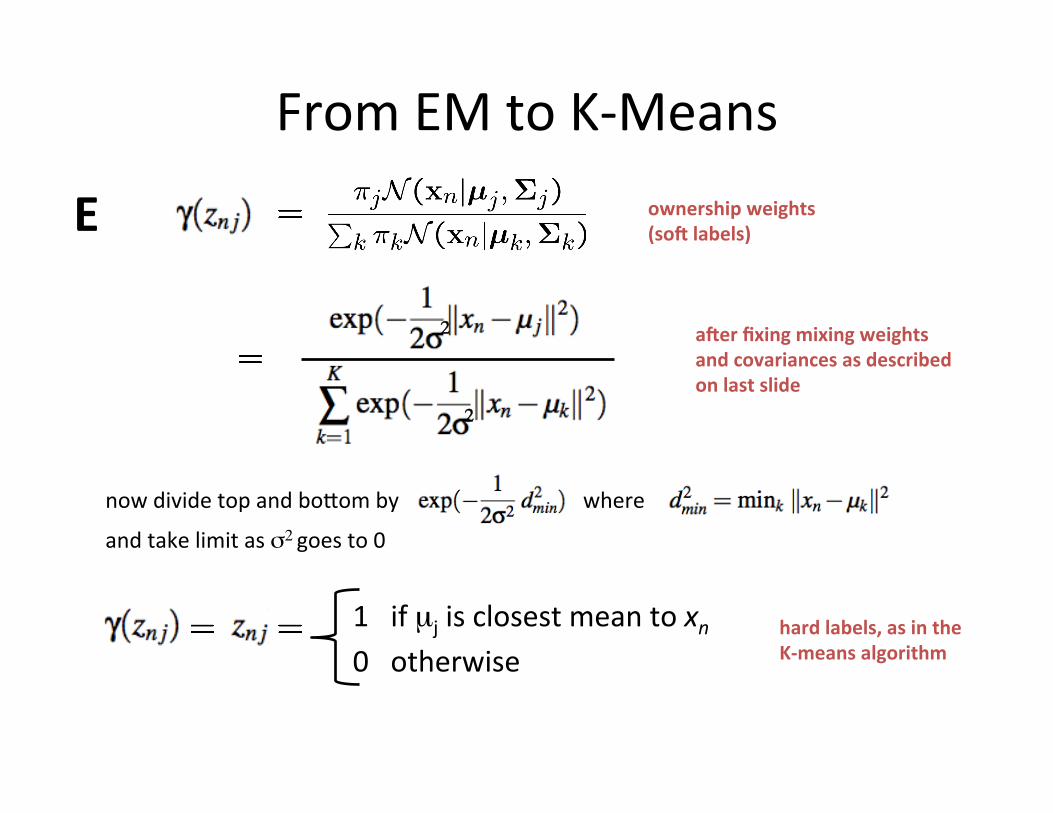
From EM to K-‐Means ownership weights (so. labels) E
a.er fixing mixing weights and covariances as described on last slide
now divide top and boVom by where
and take limit as σ2 goes to 0
1 if µj is closest mean to xn 0 otherwise
hard labels, as in the K-‐means algorithm
2
2

K-‐Means Algorithm • Given N data points x1, x2,..., xN
• Find K cluster centers µ1, µ2,..., µΚ to minimize (znk is 1 if point n belongs to cluster k; 0 otherwise)
• Algorithm: – ini3alize K cluster centers µ1, µ2,..., µΚ – repeat
• set znk labels to assign each point to closest cluster center • revise each cluster center
µj to be center of mass of points in that cluster
– un3l convergence (e.g. znk labels don’t change)
E M


![[EM-Safrida] Teori Produksi](https://static.fdocument.org/doc/165x107/55846f0dd8b42ad1588b52ac/em-safrida-teori-produksi.jpg)