FUNDAMENTALS OF SOLIDIFICATION - sina.sharif.edusina.sharif.edu/~rtavakoli/27046/kurz.pdfiv least,...
313
FUNDAMENTALS OF SOLIDIFICATION THIRD EDITION W. KURZ D.J. FISHER TRANS TECH PUBLICATIONS 1992 SWITZERLAND - GERMANY - UK - USA
Transcript of FUNDAMENTALS OF SOLIDIFICATION - sina.sharif.edusina.sharif.edu/~rtavakoli/27046/kurz.pdfiv least,...

FUNDAMENTALS OF SOLIDIFICATION
THIRD EDITION
W. KURZ
D.J. FISHER
TRANS TECH PUBLICATIONS 1992 SWITZERLAND - GERMANY - UK - USA

Ζωeigbib ι
9 °ίJ]( ω,
First edition 1984 Second edition 1986 Third revised edition 19 Reprinted 1992
W. KURZ
Professor Department of Materials Swiss Federal Institute of Technology (EPFL) Lausanne - Switzerland
D.J. FISHER
Associate editor Trans Tech Publications Ltd Aedermannsdorf - Switzerland
Bibliothek der Sektion Επergieυmwandkι g
Inventor-Nr.: -- — -Ζ~ D /,
Signαtur: 12/ 9
Copyright © 1992 Trans Tech Publications Ltd, Switzerland ISBN 0-87849-522-3
Trans Tech Publications Ltd. 1 ‚ P.O. Box 10 CH-4711 Aedermannsdorf, Switzerland
Printed in the Netherlands

FORE CORD
Solidification phenomena play an important role in many of the processes used in
fields ranging from production engineering to solid-state physics. For instance, a metal
is usually continuously cast or ingot cast before forming it into bars or sheets. The bars
then often serve as input to a sand-, permanent mould-, or precision-casting operation
while the sheet is often fabricated into useful items by welding; another solidification
process. At the other extreme, silicon is usually first prepared in the form of an impure
reduction product and then, for electronic applications, has to be purified by zone-
refining (a solidification process) and pulled, as a single crystal, from its melt.
This broad range of interest in solidification, from the large tonnages of continuously
cast products, through the intermediate weight output of superalloy precision castings,
to the relatively small quantities of high-purity crystals, means that a book such as the
present one must cater for the requirements of a very wide range of readers. To begin
with, there is the graduate or final-year undergraduate who may eventually fmd himself
dealing with any problem in the above range, and must therefore be thoroughly
conversant with the basic principles and mathematical theory of the subject. Then there
is the post-graduate researcher who may need to produce metallic specimens hiving a
well-defined microstructure and, in order to do this, must be able to bring to bear all of
the current understanding of solidification mechanisms. Finally, there is the
foundryman who would like to exert close control over a cast product, but must
contend with so many variables and unknown quantities that his work takes on the
aspects of an art. It is hoped that this book will be a value to all three groups and, at

iv
least, provide the student with an introduction to modem solidification theory; the
researcher with the fundamentals of the more quantitative models for predicting
solidification micτοstructures; and the foundryman with a framework into which he can
fit his diverse empirical observations.
The ground covered by the present introduction is essentially the same as that
covered by textbooks such as Winegard's "Introduction to the Solidification of Metals",
and Chalmers' "Principles of Solidification", both of which were published in 1964,
and Flemings' "Solidification Processing", published in 1974. Many of the 'loose
ends' of solidification theory, whose interrelationships were unclear ten or twenty years
ago, have now been drawn together and many of the qualitative arguments which were
a feature of the latter books can now be largely replaced by more quantitative models. It
is cuτently possible to present major parts of the theory as a coherent whole, and to fit
solidification microstructures into a logical framework. That is not to say that the
present-day solidification literature is immediately accessible to the newcomer. Much of
the most useful information is buried within a mass of mathematical formulae and
scattered among many journals. Therefore, the aim here has been to collect together the
key results obtained by the present and other authors, and to derive simpler solutions
whenever possible. The sources of the models used can be found in the references at
the end of each chapter but, for easier reading, are often not referred to in the text.
In order to obtain the maximum benefit from this book, the reader should note that it
is based upon a hierarchical scheme within which the subject matter can be studied at 3
levels. Firstly, an initial feeling for the subject and for the breadth of coverage, can be
obtained simply by reading the extensive figure captions. Secondly, the main text
describes the principles in more detail, but usually without deriving the necessary
equations. Thirdly, the appendices contain detailed derivations and some essential
mathematical background. It is stressed that only those readers who are specialising in
the subject would usually need to study the appendices in detail.
Within the main text, an essentially self-contained guide to the subject is presented.
That is, the reader is introduced to the mechanisms of crystal nucleation and growth
which occur at the atomic scale (chapter 2) before being shown how the form of an
initially planar solid/liquid interface evolves (chapter 3). Subsequently, the most
important single-phase (chapter 4) and multi-phase (chapter 5) solid/liquid interface
morphologies are presented. The effect, which solidification has upon the redistribution
of solute is then discussed (chapter 6). Finally, the behaviour which is to be expected at
high solidification rates is introduced in this third edition (chapter 7). This is a
topic of rapidly increasing importance. It is now possible, on the basis of work carried
out during the last few years, to discuss the effect of both high and low growth rates
upon the microstructure. Consequently, for this edition, it has been necessary to extend

V
the coverage of several of the appendices and to add a new one on the thermodynamics
of rapid solidification (appendix 6).
One subject which is not covered, due to the presently very limited understanding of
the field, is convection in the melt and its interaction with solidification microstructures.
Each chapter includes a bibliography of key references for further study, as well as
exercises which are designed to test the reader's understanding of the contents of the
preceding chapter. For certain exercises, it is advisable firstly to work through the
corresponding appendices.
The authors hope that, after reading this book, the newcomer will feel confident
when delving further into solidification-related subjects, and that the experienced
foundryman will also find some thought-provoking points.
W. Kurz, D.J. Fisher Lausanne, August 1989
ACKNOWLEDGEMENTS
The authors express their especial thanks to Dr. M. Rappaz, who contributed
generously to this textbook. Furthermore, they wish to thank Prof. G. Abbaschian, Dr.
T.W. Clyne, Prof. J. Dantzig, Dr. H. Esaka, P. Gilgien, Dr. M. Gremaud, Prof. H.
Jones, Dr. J. Lipton, Dr. M. Lorenz, Dr. P. Magnin, Prof. A. Mortensson, Prof. J.H.
Perepezko, Prof. D.R. Poirier, D. Previero, Prof. P.R. Sahm, Dr. T. Sato, J. Satsuta, Dr. P. Th€vοz, Prof. R. Trivedi, Dr. M. Wolf and Dr. M. Zimmermann for their
comments and contributions concerning the manuscript.
The invaluable aid of Dr. and Mrs. J.-P. Moinat in typesetting the equations and
editing the text, and of Mrs. E. Schlosser in preparing the diagrams is also gratefully
acknowledged.


CONTENTS
1. Introduction 1
1.1 The Importance of Solidification 1 1.2 Heat Extraction 5 1.3 Solidification Microstructures 11 1.4 Capillarity Effects 12 1.5 Solute Redistribution 15
2. Atom Transfer at the Solid/Liquid Interface 21
2.1 Conditions for Nucleation 22 2.2 Rate of Nucleus Formation 28 2.3 Interface Structure 34
3. Morphological Instability of a Solid/Liquid Interface 45
3.1 Interface Instability of Pure Substances 46 3.2 Solute Pile-Up at a Planar Solid/Liquid Interface 48 3.3 Interface Instability of Alloys 50 3.4 Perturbation Analyses 55
4. Solidification Microstructure: Cells and Dendrites 63
4.1 Constrained and Unconstrained Growth 65 4.2 Morphology and Crystallography of Dendrites 65 4.3 Diffusion Field at the Tip of a Needle-Like Crystal 69 4.4 Operating Point of the Needle Crystal - Tip Radius 74 4.5 Primary Spacing of Dendrites after Directional Growth 80 4.6 Secondary Spacing after Directional or Equiaxed Growth 85
5. Solidification Microstructure: Eutectic and Peritectic 93
5.1 Regular and Irregular Eutectics 94 5.2 Diffusion-Coupled Growth 96 5.3 Capillarity Effects 101 5.4 Operating Range of Eutectics 104 5.5 Competitive Growth of Dendrites and Eutectic 108 5.6 Peritectic Growth 111
6. Solute Redistribution 117
6.1 Mass-Balance in Directional Solidification 118 6.2 The Initial Transient 120 6.3 The Steady State 121 6.4 The Final Transient .. 122 6.5 Rapid Diffusion in the Liquid - Small Systems 122 6.6 Microsegregation 126

Contents
7. Rapid Solidification Microstructures 133
1 Departure from Local Equilibrium 134
7.2 Absolute Stability 139
7.3 Rapid Dendritic/Cellular Growth 142
7.4 Rapid Eutectic Growth 146
7.5 Intercellular Solute Redistribution 151
Summary 157
Appendices 163
1. Mathematical Modelling of the Macroscopic Heat Flux 163 2. Solute and Heat Flux Calculations Related to Microstructure Formation 177 3. Local Equilibrium at the Solid/Liquid Interface 199 4. Nucleation Kinetics in a Pure Substance 211 5. Atomic Structure of the Solid/Liquid Interface 216 6. Thermodynamics of Rapid Solidification 220 7. Interface Stability Analysis 226 8. Diffusion at a Dendrite Tip 238 9. Dendrite Tip Radius and Spacing 247 10. Eutectic Growth 261 11. Transient in Solute Diffusion 275 12. Mass Balance Equations 280 13. Homogenisation of Interdendritic Segregation in the Solid State 289 14. Relevant Physical Properties for Solidification 293
Symbols 295
Index 301

CHAPTER ONE
INTRODUCTION
1.1 The Importance of Solidification
Solidification is a phase transformation which is familiar to everyone, even if the
only acquaintance with it involves the making of ice cubes. It is relatively little
appreciated that the manufacture of almost every man-made object involves
solidification at some stage.
The scope ,of this book is restricted mainly to a presentation of the theóry of
solidification as it applies to the most widely-used group of materials, i.e. metallic
alloys. Here, solidification is generally accompanied by the formation of crystals; an
event which is much rarer during the solidification of ceramic glasses or polymers.
Solidification is of such importance simply because one of its major practical
applications, namely casting, is a very economic method of forming a component if the

liquid
20 30
1/τ
10-e 0 10 40 50
τ .10 .05 .033 .025 .02
Ο a
2 Fundamentals of Solidification
Figure 1.1 Dynamic Viscosity as a Function of Temperature
The fundamental advantage of solidification, as a forming operation, is that it permits metal to be shaped with a minimum of effort since the liquid metal offers very little resistance to shear stresses. When the material solidifies due to a decrease in the temperature,r, its viscosity increases continuously (glass formation) or discontinuously (crystallisation), by over 20 orders of magnitude, to yield a strong solid, the viscosity of which is defined arbitrarily to be greater than 1014Pas. (The reduced temperature,r, is used here since it leads to a single curve which is applicable to many substances. The suffix, f or v, indicates the melting point or boiling point, respectively.) [D.Turnbull, Transactions of the Metallurgical Society of AIMS 221 (1961) 422].
melting point of the metal is not too high. Nowadays, cast metal products can be
economically produced from alloys having melting points as high as 1660°C (Ti).
In the case of metals, melting is accompanied by an enormous decrease in viscosity,
of some twenty orders of magnitude, as illustrated in figure 1.1. Thus, instead of
expending energy against the typically high flow stress of a solid metal during forging
or similar processes, it is only necessary to contend with the essentially zero shear
stress of a liquid. If the properties of castings were easier to control, then solidification
would be an even more important process. In this respect, solidification theory plays a
vital role since it forms the basis for influencing the microstructure and hence improving
the quality of cast products.
The effect of solidification is most evident when casting is the final operation since
the resultant properties can depend markedly upon the position in the casting

50 100 150
d(mm)
12
8 α
4 ω
0
400 cv ε Ζ Σ 200 a ~ b
0
N Ε \
Introduction
3
Figure 1.2 Alloy Properties as a Function of Position in a Casting
The use of casting as a production route unfortunately poses its own problems. One of these is the local variation of the microstructure, leading to compositional variations, and this is illustrated for example by the dendrite arm spacing,λ2, measured as a function of the distance, d, from the surface of the casting. This can lead to a resultant variation in properties such as the ultimate tensile strength and the elongation. Like the weakest link in a chain, the inferior regions of a casting may impair the integrity of the whole. Thus, it is important to understand the factors which influence the microstructure. Finer microstructures generally have superior mechanical properties and finer structures, in turn, generally result from higher solidification rates. Such rates are found at small distances from the surface of the mould, in thin sections, or at laser-remelted surfaces. [MC. Flemings, Solidification Processing, McGraw-Hill, New York, 1974].
(Fig. 1.2). Its influence is also seen in a finished product, even after heavy working,
since a solidification structure and its associated defects are difficult to eliminate once
they are created. Solidification defects tend to persist throughout subsequent operations
(Fig. 1.3). Good control of the solidification process at the outset is therefore of utmost
importance.
Some important processes which involve solidification are:
Casting: continuous-
ingot-
form-
precision-
die-

Soldering/Brazing
Rapid Sοlidificatiοn Processing:
Fundamentals of Solidification
Welding:
Directional Solid(/ication:
arc-
resistance-
plasma-
electron beam-
laser-
friction- (including the
micro-mechanisms of wear
melt-spinning
planar-flow casting
atomisation
bulk undercooling
surface remelting
Bridgman
liquid metal cooling
Czochralski
electroslag remelting
Figure 1.3 Effect of Deformation upon a Cast Microstructure
Often, casting is not the final forming operation. However, subsequent deformation is not a very efficient method of modifying the as-cast microstructure since any initial heterogeneity exhibits a strong tendency to persist. Thus, during the rolling of this L-shaped profile which contains a heavily segregated central region, the latter defect survives the many stages between the cast billet and the final product. This example emphasises the fact that an effective control of product quality must be exercised during solidification. [A.J. Pokorny, De Ferri Metallographia, Vol. III, Luxembourg, 1966, p. 287].

Iiitroduction 5
In addition, the crystallisation of certain pure substances is of great importance. For
example, the preparation of semiconductor-grade silicon crystals is an essential step in
modern solid-state physics and technology. The production of integrated circuits; the
basis of any new electronic device (radio, watch, computer, etc), requires the
preparation of large single crystals of very high perfection, containing a controlled
amount of a uniformly distributed dopant. At the moment, such a crystal can only be
produced by growth from the melt. Indeed, the requirements of semiconductor physics
have enormously influenced solidification theory and practice. Therefore, during the
past thirty years solidification has evolved from being a purely technological, empirical
field, to become a science.
Historically, simple cast objects (in copper) first appeared before about 4000BC and
were, no doubt, a natural by-product of the potter's skill in handling the clay used in
furnace-and mould-making. The production of the renowned and highly sophisticated
bronze castings of China began in about 1600ΒC. However, it is probable that the
technique had originally been imported from elsewhere. For instance, the lost-wax
process was developed in Mesopotamia as long ago as 3000ΒC. Iron-casting in China
began in about 500BC, but in Europe cast iron did not appear until the 16th century,
and achieved acceptance as a constructional material, in England in the 18th century,
only under the impetus of the industrial revolution.
Much of the delay in exploiting cast materials probably originated from the complete
lack of understanding of the nature of solidification phenomena and of the
microstructures produced. In particular, the facets of fracture surfaces were invariably
taken to indicate the nature of the 'crystals' of which a casting was composed. In the
absence of an adequate picture of the solidification process, casting was bound to
remain a black art rather than a science, and vestiges of this attitude still remain today.
1.2 Heat Extraction
The various solidification processes mentioned above involve extraction of heat from
the melt in a more or less controlled manner. Heat extraction changes the energy of the
phases (solid and liquid) in two ways:
1. There is a decrease in the enthalpy of the liquid or solid, due to cooling, which is
given by: ∆H = JcdT
2. There is a decrease in enthalpy, due to the transformation from liquid to solid,
which is equal to the latent heat of fusion, ∆Hf
Heat extraction is achieved by applying a suitable means of cooling to the melt in
order to create an external heat flux, Qe. The resultant cooling rate, dT/dt, can be

6 Fundamentals of Solidification
deduced from a simple heat balance if the metal is isothermal (low cooling rate) and the
specific heats of the liquid and the solid are the same. Using the latent heat per unit
volume, ∆hf= ∆HJ/vm (defined to be positive for solidification), and also the specific
heat per unit volume, c, in order to conform with the dimensions of the other factors,
then:
= - ε(~~tT ) + ∆h f(.ά.)
so that:
dt — qe( ς)+( dt)\~)
The first term on the right-hand-side (RHS) of equation 1.1 reflects the effect of
casting geometry (ratio of surface area of the casting, A', to its volume, v) upon the
extraction of sensible heat, while the second term takes account of the continuing
evolution of latent heat of fusion during solidification. It can be seen from this equation
that, during solidification, heating will occur if the second term on the RHS of equation
1.1 becomes greater than the first one. This phenomenon is known as recalescence. For
an alloy, where solidification occurs over a range of temperatures, the variation of the
fraction of solid as a function of time must be calculated from the relationship:
dfs = ~ dT ~ ~dfs ~ dt dt dT
since fs is a function of temperature. In this case:
— qeιyε ~ [1.2]
1 - (&‚ ~ dTs
It is seen that solidification decreases the cooling rate since dfs/dΤ is negative.
Figure 1.4 illustrates two fundamentally different solidification processes. In figure
1 .4a, the heat is extracted in an almost steady manner by moving the crucible at a fixed
rate, V', through the temperature profile imposed by the furnace. Such a process is
usually used for single crystal growth or directional solidification. It permits the growth
rate of the solid, V (which is not necessarily equal to the rate of crucible movement - see
exercise 1.9), and the temperature gradient, G, to be separately controlled. If V is not
too high, both the heat flux and the solidification are unidirectional. The cooling rate at a
given location and time is given by:

Introduction 7
_d Φ t
ii
1
ins
ula
tio
n
S
I VI
chill
a b
Figure 1.4 Basic Methods of Controlled Solidification
Without heat extraction there is no solidification. The liquid must be cooled to the solidification temperature and then the latent heat of solidification appearing at the growing solid/liquid interface must be extracted. There are several methods of heat extraction. In directional (Bridgman-type) solidification (a): the crucible is drawn downwards thrόugh a constant temperature gradient, G, at a uniform rate, V', and therefore the microstructure is highly uniform throughout the specimen. The method is restricted to small specimen diameters and is expensive because it is slow and, paradoxically, heat must be supplied during solidification in order to maintain the imposed positive temperature gradient. For these reasons, it is employed only for research purposes and for the growth of single crystals. In directional casting (b), the benefits of directionality, such as a better control of the properties and an absence of detrimental macrosegregation, are retained but the microstructure is no longer uniform along the specimen because the growth rate, V, and the temperature gradient decrease as the distance from the chill increases. The process is cheaper than that of (a) and is used for the directional solidification of gas-turbine blades, for example. Combined with proper alloy development, these processes result in a higher efficiency and a longer life for the gas-turbines of aircraft.
= lá is+ ε — +ε ~ αr az» ~
Τ' ι1ε s +ε = G·V Ι s+ ε [1.3]
where the time-dependent position of the solid/liquid interface is s = z' — z, and i is the
coordinate with respect to the system (the crucible), while z is the coordinate with
respect to the moving s/l interface (Fig. 1.4; see also figure Α2.2), and ε is a"small
quantity with respect to s. Here, V is the rate of movement of the s/l interface and G is
the thermal gradient in the liquid when z = s + ε (also called G1) or the thermal
gradient in the solid when z' = s —ε (called Gs). Due to differences in the conductivity of
solid and liquid and due to the evolution of latent heat at a moving interface, G1 * G.

columnar zone
8 Fundamentals of Solidification
mushy zone
cas ing
Figure 1.5 Solidification in Conventional Castings and Ingots
In the vast majority of castings, no directionality is imposed upon the overall structure, but the local situation can be seen to be equivalent to that existing in directional casting (Fig. 1.4b). This is true of the way in which the solid advances inwards from the mould wall to form a columnar zone. During the growth of the columnar zone, three regions can be distinguished. These are the liquid, the liquid plus solid (so-called mushy zone), and the solid region. The mushy zone is the region where all of the microstructural characteristics are determined, e.g. the shape, size, and distribution of concentration variations, precipitates, and pores. An infinitesimally narrow volume element which is fixed in the mushy zone and is perpendicular to the overall growth direction permits a description of the microscopic solidification process and therefore of the scale and composition of the microstructure.
For reasons of simplicity, the temperature gradient in the liquid will be mostly used in
this book and written as G = G/. However, one has to bear in mind that under certain
conditions (as explained in chapter 3) the physically meaningful temperature gradient is
the mean gradient, G = (Gsκs+Gικι)/(κs+κι). Another directional casting process is illustrated by figure 1.4b. Here, heat is
extracted via a chill and, as in figure 1.4α, growth occurs in a direction which is

Introduction 9
parallel, and opposite, to the heat-flux direction. In this situation, the heat-flux
decreases with time as do the coupled parameters, G and V. Thus T also varies. Heat
flow in the mould/metal system leads to an expression for the position, s, of the
solid/liquid interface, which is of the type (appendix 1):
s = Ktl/2
[1.4]
This equation is exact only if the melt is not superheated, if the solid/liquid interface is
planar, and if the surface temperature of the casting at the chill drops immediately, at
t = 0, to a constant value. Figure 1.4b can be regarded as being a volume element in a
conventional casting (Fig. 1.5). The difference between the figures is the presence of a
dendritic morphology at the solid/liquid interface shown schematically in figure 1.5.
equiaxed zone
outer inner
a b
columnar zone
Figure 1.6 Structural Zone Formation in Castings
Firstly, solid nuclei appear in the liquid at, or close to, the mould wall. For a short time, they increase in size and form the outer equiaxed zone. Then, those crystals (dendrites) of the outer equiaxed zone which can grow parallel and opposite to the heat flow direction will advance most rapidly. Other orientations tend to be overgrown, due to mutual competition, leading to the formation of a columnar zone (a). Beyond a certain stage in the development of the columnar dendrites, branches which become detached from the latter can grow independently. These tend to take up an equiaxed shape because their latent heat is extracted radially through the undercooled melt. The solidified region containing them is called the inner equiaxed zone (b). The transition from columnar to equiaxed growth is highly dependent upon the degree of convection in the liquid. In continuous casting machines, electromagnetic stirring is often used to promote this transition and lead to superior soundness at the ingot centre.

7
7
b
d
a
F
ε
10 Fundamentals of Solidification
This morphology depends (chapter 4) upon the alloy composition, and upon G and V.
If it is assumed, for simplicity, that the dendrites can be represented by plates#, then
solidification on a microscopic scale again takes place directionally (perpendicular to the
primary growth axis of the dendrites, as shown in the upper insert of figure 1.5). This
representation permits a simple estimation of interdendritic microsegregation (chapter
6).
1mm
Figure 1.7 Solid/Liquid Interface Morphology and Temperature Distribution
In the case of a pure metal (a,b) which is solidifying inwards from the mould wall, the columnar grains (a) possess an essentially planar interface, and grοω in a direction which is antiparallel to that of the heat flοω. Within the equiaxed region of pure cast metal (b), the crystals are dendritic and grοω radially in the same direction as the heat flοω. When alloying elements or impurities are present, the morphology of the columnar crystals (c) is generally dendritic. The equiaxed morphology in alloys (d) is almost indistinguishable from that in pure metals, although a difference may exist in the relative scale of the dendrites. This is because the growth in pure metals is heat-flow-controlled, while the growth in alloys is mainly solute-diffusion-controlled. Note that in columnar growth the hottest part of the system is the melt, while in equiaxed solidification the crystals are the hottest part. It follows that the melt must always be cooled to below the melting point (i.e. undercooled) before equiaxέd crystals can grοω.
Plate-like primary crystal morphologies are often observed during solid-state precipitation. When metallic primary crystals grοω into a melt, they are always rod-like rather than plate-like in form and possess many branches, leading to the characteristic dendrite form.

a
l b C d
7οο :fi~
υ 600 ο Η
500 0 20 40
C (wt%Cu)
Θ
Introduction 11
Figure 1.8 Principal Alloy Types
It is important to understand how the various microstructures are influenced by the alloy composition and by the solidification conditions. Fortunately, this can usually be reduced to the study of two basic morphological forms: dendritic and eutectic. Thus, one can distinguish: a) pure substances, which solidify in a planar or dendritic manner, b) solid-solution dendrites (with or without interdendritic precipitates), c) dendrites plus interdendritic eutectic, and d) eutectic. The latter group includes the familiar 'cast iron' and 'plumber's solder' type of alloy. In general, the design of casting alloys is governed by the twin aims of obtaining the required properties and good castability (i.e. easy mould filling, low shrinkage, small hot tearing tendency, etc.). Castability is greatest for pure metals and alloys of eutectic composition. The diagram represents the Al-Cu system between Al and the intermetallic (theta) phase, Al2Cu.
1.3 Solidification Microstructures
In an ingot or casting, three zones of solidification behaviour can generally be
distinguished (Fig. 1.6). At the mould/metal interface, the cooling rate is at its highest
due to the initially low relative temperature of the mould. Consequently, many small
grains having random orientations are nucleated at the mould surface and an 'outer
equiaxed' zone is formed. These grains rapidly become dendritic, and develop `arms
which grow along preferred crystallographic directions (<001> in the case ofcubic
crystals). Competitive grοωth between the randomly oriented outer equiaxed grains
causes those which have a preferred growth direction (parallel and opposite to the
direction of heat flow) to eliminate the others. This is because their higher grοωth rate
allows them to dominate the solid/liquid interface morphology, thus leading to the
formation of the characteristic columnar zone. It is often observed that another equiaxed

12 Fundamentals of Solidification
zone forms in the centre of the casting, mainly as a result of the growth of detached
dendrite arms within the remaining, slightly-undercooled liquid.
Figure 1.7 shows the temperature fields in the various cast structures which one
might encounter. These are planar interface (columnar grains - a) or thermal dendrites
(equiaxed grains - b) in pure materials, and solutal (constitutional) dendrites in alloys
(c,d). It can be seen that columnar grains must always grow out from the mould (which
is the heat sink) in a direction which is opposite to that of the heat flow, while equiaxed
grains grow in a supercooled melt which acts as their heat sink. Thus, the growth
direction and the heat flow direction are the same in equiaxed growth.
The form of a solidification microstructure depends not only upon the cooling
conditions, but also upon the alloy composition (Fig. 1.8). There are essentially two
basic growth morphologies which can exist during alloy solidification. These are the
dendritic and eutectic morphologies (peritectic alloys grow in a dendritic manner).
Generally, a mixture of both morphologies will be present. It is reassuring, in the face
of the apparent microstructural complexity, to remember that it is only necessary to
understand these two growth forms in order to interpret the solidification microstructure
of almost any alloy.
Figure 1.9 illustrates the various stages of equiaxed solidification — from nucleus to
grain — for the two major growth morphologies: dendrites and eutectic. Each grain has
one nucleus at its origin. (In the literature of cast iron, an eutectic grain is often called an
eutectic cell. This definition will not be adopted because the term, cell, is here reserved
for another morphology.)
The transformation of liquid into solid involves the creation of curved solid/liquid
interfaces (leading to capillarity effects) and the microscopic flow of heat (and also
solute in the case of alloys).
1.4 Capillarity Effects
With any solid/liquid interface of area, A, is associated an excess (interface) energy
which is required for its creation. Therefore, heterogeneous systems or parts of systems
which possess a high A/ν ratio will be in a state of higher energy and therefore unstable
with respect to a system of lower A/v ratio. The relative stability can be expressed by
the equilibrium temperature between both phases (melting point). As shown in appendix
3, the change in melting point due to this curvature effect, often called the curvature or
Gibbs-Thomson undercooling, is given by:
∆Τ = K Γ [1.5]

Ο
Ο 0
SD
αο φσ
αα
a b
~
100 µm
0 0
0
Introduction 13
tf
Figure 1.9 Process of Equiawed Solidification of Dendrites and Eutectic
In each case, single-phase nuclei form initially. In pure metals or single-phase alloys (a), the nuclei then grοω into spherical crystals which rapidly become unstable and dendritic in form. These dendrites grοω freely in the melt and finally impinge on one another. In a pure metal after solidification no trace of the dendrites themselves will remain, although their points of impingement will be visible as the grain boundaries. In an alloy, the dendrites will remain visible after etching due to local composition differences (microsegregation). In an eutectic alloy (b), a second phase will soon nucleate on the initial, single-phase nucleus. The eutectic grains then continue to grοω in an essentially spherical form. In a casting, both growth forms, dendritic and eutectic, often develop together. Note that each grain originates from a single nucleus.

14 Fundamentals of Solidification
Note that the curvature, K, and the Gibbs-Thomson coefficient, Γ, are here defined
so that a positive undercooling (decrease in equilibrium melting point) is associated with
a portion of solid/liquid interface which is convex towards the liquid phase. The
curvature can be expressed as (appendix 3):
κ= = ί ± ί [ 1.6] dv rl r2
where r1 and r2 are the principal radii of curvature#. Thus, the total curvature of a
sphere is 2/r and that of a cylindrical surface is 1/r. The Gibbs-Thomson coefficient is
given by:
Γ _ σ ∆sf
[1.7]
For most metals, Γ is of the order of 10-7Κm. Hence, the effect of the solid/liquid
interface energy, σ, only becomes important for morphologies which have a radius that
is less than about 10 gm. These include nuclei, interface perturbations, dendrite tips,
and eutectic phases (Fig. 1.10).
a b
C
d
Figure 1.10 The Scale of Various Solid/Liquid Interface Morphologies
Solidification morphologies are determined by the interplay of two effects acting at the solid/liquid interface. These are the diffusion of solute (or heat), which tends to minimise the scale of the morphology (maximise curvature), and capillarity effects which tend to maximise the scale. The crystal morphologies actually observed are thus a compromise between these two tendencies, and this can be shown with respect to nucleation (a), interface instability (b), dendritic growth (c), and eutectic growth (Φ.
The two principal radii of curvature are the minimum and maximum values for a given surface. It can be shown that they lie in planes always perpendicular to each other.

Introduction 15
1.5 Solute Redistribution
The creation of a crystal from an alloy melt causes a local change in the composition.
This is due to the equilibrium condition for a binary system containing two phases:
Αµi = µs , µs = µs [1.8]
(appendix 3). The difference in composition at the growing interface, assuming that
local (i.e. at the interface) equilibrium exists in metals under normal solidification
conditions, can be described by the distribution coefficient under isothermal and
isobaric conditions (Fig. 1.11):
k CS _ \ςι / r,Ρ [1.9]
Τι
Τ 3
Co Co/k
Figure 1.11 Solid/Liquid Equilibrium
In order to simplify the mathematical treatment of solidification processes, it is generally assumed that the liquidus and solidus lines of the phase diagram are straight, and therefore that the distribution coefficient, k, and the liquidus slope, m, are constant. The characteristic properties of the system are defined in the text (equations 1.9 to 1.11),

16 Fundamentals of Solidification
In most of the theoretical treatments to be presented later, the solidus and liquidus
lines will be assumed to be straight. This means that k and m, the liquidus slope, are
then constant. This violates the condition for thermodynamic equilibrium (equation 1.8)
but often makes theoretical analyses more tractable. However, if the variation in
composition is large, e.g. due to a large variation of growth rate, this assumption might
lead to wrong results. Throughout this book, m is defined so that the product, (k-1)m, is positive. That is,
m is defined to be positive when k is greater than unity, and to be negative when k is
less than unity. Two other important parameters of an alloy system are shown in figure
1.11. These are the liquidus-solidus temperature interval for an alloy of composition,
Co:
∆Το = — m ∆Co = (Τ, — Τ ) [ 1.10]
and the concentration difference between the liquid and solid solute contents at the
solidus temperature of the alloy:
∆Co = C0 (1—k) k
Under rapid solidification conditions equation 1.8 may no longer be satisfied, and k
then becomes a function of V. This so-called non-equilibrium solidification can lead to a
highly supersaturated crystal (see chapter 7).
In later chapters it will be shown how the above parameters influence the
solidification microstructure. Meanwhile, the starting point of solidification (nucleation)
will be considered briefly, and a look will be taken at the mechanisms by which atoms
in the melt become part of the growing crystal.
Bibliography
Solidification Microstructure and Properties
M.C.Flemings, Solidification Processing, McGraw-Hill, New York, 1974, p. 328.
W.Kurz, P.R.Sahm, Gerichtet erstarrte eutektische Werkstoffe, Springer, Berlin,
1975.
G.F.Bolling, in Sοlidifϊcatiοn, American Society for Metals, Metals Park, Ohio, 1971,
p. 341.
J.F.Burke, M.C.Flemings, A.E.Gorum, Solidification Technology, Brook Hill, 1974.

Introduction 17
Analytical Solutions to Heat Flow Problems in Solidification
H.S.Carslaw & J.C.Jaeger, Conduction of Heat in Solids, 2nd Edition, Oxford
University Press, London, 1959.
G.H.Geiger, D.R.Poirier, Transport Phenomena in Metallurgy, Addison-Wesley,
1973.
J.Szekely, N.J.Themelis, Rate Phenomena in Process Metallurgy, Wiley - Interscience,
New York, 1971.
Capillarity Effects
W.W.Mullins, in Metal Surfaces - Structure, Energetics, and Kinetics, ASM, Metals
Park, Ohio, 1963, p. 17.
R.Trivedi, in Lectures on the Theory of Phase Transformations (Edited by
H.I.Aaronson), TMS of ΜΜΕ, New York, 1975, p. 51.
Thermodynamics of Solidification
J.C.Baker, J.W.Cahn, in Solidification, American Society for Metals, Metals Park,
Ohio, 1971, p. 23.
M.C.Flemings, Solidification Processing, McGraw-Hill, 1974, p. 263.
J.S.Kirkaldy, in Energetics in Metallurgical Phenomena - Volume IV, (Edited by
W.M.Mueller), Gordon & Breach, New York, 1968, p. 197.
M.Hillert, in Lectures on the Theory of Phase Transformations (Edited by
H.I.Aaronson), TMS of AIMS, New York, 1975, p. 1.
Casting Techniques
R.Flinn, in Techniques of Metals Research - Volume I, (Edited by R.F.Bunshah),
Wiley, New York, 1968.
F.L.Versnyder, M.E.Shank, Materials Science and Engineering 6 (1970) 213.
T.F.Bower, D.A.Granger, J.Keverian, in Solidification, American Society for Metals,
Metals Park, Ohio, 1971, p. 385.
Phase Diagrams
M.Hansen, Constitution of Binary Alloys, McGraw-Hill, New York, 1958.
T.B.Massalski et al. (Eds.), Binary Alloy Phase Diagrams, ASM, Metals Park, Ohio,
1986.
Metals Handbook - Volume 8, ASM, Metals Park, Ohio.
Rapid Solidification
J.C.Baker, J.W.Cahn, in, Solidification, ASM, Metals Park, Ohio, 1971, p. 23.
W.J.Boettinger, S.R.Cońell, R.F.Sekerka, Material Science and Engineering 65
(1984) 27.

18 Fundamentals of Solidification
H.Jones, Rapid Solidification of Metals and Alloys, The Institution of Metallurgists,
London, 1982.
Exercises
1.1 Discuss the shape of the upper surface of the ingot in figure 1.6. What would
happen if the solidifying material was one of the following substances: water, Ge,
Si, Bi?
1.2 From a consideration of the volume element in the mushy zone of figure 1.5
(upper part), define the local solidification time, tf, in terms of the dendrite growth
rate, V, and the length, a, of the mushy zone.
1.3 Sketch η—τ diagrams for the crystallisation of a pure metal and for an alloy, and
comment on their significance in each case.
1.4 Equiaxed dendrites are developing freely in an undercooled melt. Discuss the
direction of movement of the equiaxed dendrites in a quiescent melt. Where would
most of them be found in solidifying melts of a) steel, b) Bi?
1.5 Sketch two different phase diagrams having a positive and a negative value of m.
Show that the product, m(k - 1), is always positive.
1.6 Using data from "Constitution of Binary Alloys" (M.Hansen and K.Anderko,
McGraw-Hill, New York, 1958) or other similar phase-diagram compilations,
estimate the distribution coefficient, k, of S in Fe at temperatures of between 1500
and 988°C, and of Cu in Ni at temperatures of between 1400 and 1300°C. Discuss
the validity of the assumption that k is constant in these systems.
1.7 A molten alloy, like any liquid which has local density variations, will tend to
exhibit the motion known as natural convection. What is the origin of this
convection in a) pure metals, b) alloys? Discuss your conclusions with regard to
various alternative solidification processes such as upward (as opposed to
downward) directional solidification (Bridgman - Fig. 1.4), and casting
(Fig. 1.5).
1.8 Give possible reasons for the good mould-filling characteristics which are
exhibited by pure metals and eutectic alloys during the casting of small sections.
Discuss them with regard to the interface morphology shown in figure 1.7.

Inlroduction 19
1.9 Figure 1.4 illustrates two directional solidification processes which differ with
respect to their heat transfer characteristics. In one case, a steady-state behaviour
is established after some transient changes. In the other case, changes continue to
occur with the passage of time. One process is not limited with regard to the
length of the product, but is limited by its diameter. The other process is not
affected by the diameter, but rather by the specimen length. Sketch heat flux lines,
and G and V values as a function of t for both cases and relate them to the
described characteristics of the two processes. Note that, in directional
solidification, the temperature gradient in the liquid at the solid/liquid interface
must always be positive, as shown in figure 1.7a,c.
1.10 Illustrate the changes in the temperature distribution of a casting as a function of
time between the moment of pouring of a pure superheated melt and the
establishment of the situation shown in figures 1 .7a and b. Discuss the
fundamental differences between a and b.


CHAPTER TWO
ATOM TRANSFER AT THE SOLID/LIQUID INTERFACE
From a thermodynamic point of view, solidification requires a heat flux from the
system to the surroundings which changes the free energies, and therefore the relative
thermodynamic stability, of the phases present. From the same point of view,
thermodynamically stable phases are more likely to be observed, but the transformation
of one phase into another requires rearrangement of the atoms. This may involve a
relatively short-range (atomic) rearrangement to form a new crystal structure, as in the
case of a pure substance. Alternatively, atomic movement may be required overmuch
larger, but still microscopic, distances as in the case of alloy solidification where'mass
diffusion controls the transformation. Because of these atomic movements,
solidification will always require some irreversible departure from equilibrium in order
to drive the process.

22 Fundamentals of Solidification
Like chemical reactions, phase transformations are driven by thermal fluctuations and
can only occur when the probability of transfer of atoms from the parent phase to the
product phase is higher than that for the opposite process. However, before this stage is
reached, it is necessary that some of the new phase, to which atoms of the parent phase
can jump, should already exist. Therefore, stable regions of the new phase have to
form. In liquid metals, random fluctuations may create minute crystalline regions
(clusters, embryos) even at temperatures greater than the melting point, but these will
not be stable. They continue to be metastable below the melting point because the
relatively large excess energy required for surface creation tends to weight the 'energy
balance' against their survival when they are small.
Once nucleation has occurred, atom transfer to the crystals has to continue in order to
ensure their growth. The mechanisms involved during this second stage are discussed
in section 2.3.
2.1 Conditions for Nucleation
It is inherently difficult to observe the process of nucleation because it involves such
small clusters of atoms. Consequently, only extremely careful comparison of theoretical
models and experimental results can clarify the very first stages of solidification. As
demonstrated in figure 2.1 nucleation begins at some degree of undercooling, ∆Τ =
∆Τ , which for metals is generally very small in practical situations. The initially
small grains which begin to grow do not appreciably modify the cooling rate imposed
by the external heat flux, Qe. Increasing the undercooling has the effect of markedly
increasing the nucleation rate, I, and also the growth rate, V, of the dendrites. The
overall solidification rate approaches a maximum value when the internal heat flux (qj),
which is proportional to the latent heat of fusion and the volume rate of transformation,
.f,(=dfs/dt), is equal to the external one (qe) (equation 1.1). Here, Τ = Ο. During the
first stage of equiaxed solidification, which is essentially nucleation-controlled, the
volume fraction of solid is still very small. After some time, the temperature of the
system has risen above the nucleation temperature and the second stage of solidification
is growth-controlled. The number of grains present thus remains essentially constant
and solidification proceeds first via the lengthening of dendrites, and then via dendrite
arm thickening once the grains are in contact.
From this sort of consideration, it is possible to deduce that nucleation is the
dominant process at the beginning of solidification and leads very rapidly to the
The undercooling, ∆Τ, is usually defined as the temperature difference between the equilibrium temperature of a system and its actual temperature. The latter is lower than the equilibrium temperature when the melt is undercooled. In this case, ∆Τ is greater than zero. The term, supercooling, is often used interchangeably with undercooling in the literature.

Atom Transfer at the Solid/Liquid Interface 23
a
b
.Η
∆Τ<;
1
Η
t f
1
0
0
1
1
Ζ
0
C
d
e
,
Ν
Figure 2.1 Thermal History of Equiaxed Dendritic Solidification
The above temperature-time curve is one which might well be obtained during a solidification sequence such as that pictured in figure 1.9α. The usual cooling curve (a) begins to deviate slightly; at the undercooling where nucleation occurs, ∆Τ4. At this point, the first fraction of solid, fs, appears (d). With further cooling, the nucleation rate, I, rapidly increases to a maximum value (e). At the minimum in the temperature-time curve, the growth rate, V. of the grains (i.e. of the dendrite tips) is at its highest. The subsequent increase in temperature is due to the high internal heat flux, q;, arising from the late of transformation, fs(= dfs/tit), and the latent heat released (c). (The maximum of the temperature can lie above the nucleation temperature.) Note that / is much more sensitive to temperature changes than is V (e). Most of the solidification which takes place after impingement of the grains involves dendrite arm coarsening at a tip growth rate, V, equal to zero. During this time interval, the number of grains, N, remains constant.

24 Fundamentals of Solidification
establishment of the final grain population, with each nucleus forming one equiaxed
grain of the type shown in figure 1.7b or d. Note that even in the case of columnar
solidification, the very first solid in a casting always appears in the form of equiaxed
grains (Fig. 1.6). The conditions leading to nucleation are therefore of utmost
importance in determining the characteristics of any cast microstructure.
In phase changes such as solidification, which are discontinuous, the transformation
process cannot occur at any arbitrarily small undercooling. The reason for this arises
from the large curvature of the interface associated with a crystal of atomic dimensions.
This curvature markedly lowers the equilibrium temperature (appendix 3) so that, the
smaller the crystal, the lower is its melting point. This occurs because the small radius
of curvature creates a pressure difference between the two phases which is of the order
of 100MPa (lkbar) for a crystal radius of 1nm. The equilibrium melting point of the
system is thus lowered by an amount, ∆Tr. The critical size, r°, of a crystal, i.e. the size
which allows equilibrium between the curved crystal and its melt, can be easily
calculated. For a sphere (appendix 3) it is:
∆Τ = ΚΓ = 2r r r°
and
ra _ 2Γ 2σ _
∆Τ ∆Τ ∆s
r f.
This relationship indicates that, the smaller the difference (undercooling) between the
melting point and the temperature of the melt, the larger will be the size of the
equilibrium crystal. For nucleation of a spherical crystal of radius, r, to occur, a number
of atoms, each of volume, v', given by:
4r3 η — 3 ν'
[2.2]
have to arrange themselves on the sites of the corresponding solid crystal lattice. It is
evident that the probability of this event occurring is very small for large values of r°,
i.e. at small undercoolings (equation 2.1).
As shown in figure 2.2, the critical condition for the nucleation of 1 mole is derived
by summing the interface and volume terms for the Gibbs free energy:
∆G = ∆G1 + ∆G = σΑ + ∆g•ν [2.3]
where σ is the solid/liquid interface energy and ∆g is the Gibbs free energy difference
[2.1]

d - ti
- t2
τ
Θ b
0 ∆Gν
Τ = Tf
Atom Transfer at the Solid/Liquid Interface 25
a 0
- ∆G° ε
Ρ°
Ρ
Figure 2.2 Free Energy of a Crystal Cluster as a Function of its Radius
The phenomenon of nucleation of a crystal from its melt depends mainly on two processes: thermal fluctuations which lead to the creation of variously sized crystal embryos (clusters), and creation of an interface between the liquid and the solid. The free energy change, ∆G, which is associated with the first process is proportional to the volume transformed. That is, it is proportional to the cube of the cluster radius. The free energy charge, ∆G1, which is associated with the second process is proportional to the area of solid/liquid interface formed. That is, it is proportional to the square of the cluster radius. At temperatures, T, greater than the melting point (a), both the volume free energy (∆G) and the surface free energy (∆G) increase monotonically with increasing radius, r. Therefore, the total free energy, ∆G, which is their sum, also increases monotonically. At the melting point (b), the value of ∆G still increases monotonically since it is only slightly temperature dependent. Because, by definition, thermodynamic equilibrium exists between the solid and liquid at the melting point, the value of ∆G is zero. Hence ∆G again increases monotonically with increasing radius. At a temperature below the equilibrium melting point (c), the sign of ∆G is reversed because the liquid is now metastable, while the behaviour of ∆G; is still the same as in (a) and (b). However, ∆G has a 3rd-power dependence on the radius while ∆G has only a 2nd-power dependence. At small values of the radius, the absolute value of ∆G is less than that of ∆G, while at large values of r the cubic dependence of ∆G predominates. The value of ∆G therefore passes through a maximum at a critical radius, r°. Fluctuations may move the cluster backwards and forwards along the ∆G—r curve (c) due to the effect of random additions to, or removals of atoms from, the unstable nucleus (d). When a fluctuation causes the cluster to become larger than r°, growth will occur due to the resultant decrease in the total free energy. Thus, an embryo or cluster (r<r°) becomes a nucleus (r = r°) and eventually a grain (r » r°).

n°
∆G°
26 Fundamentals of Solidification
between the liquid and solid per unit volume. Again assuming a spherical form
(minimum Α/ν ratio) for the nucleus,
∆G = σ4nr2 + ∆g 4nr
3
3 [2.4]
The Gibbs free energy per unit volume, ∆g, is proportional to ∆Τ (appendix 3):
∆g = — ∆sf ∆Τ [2.5]
The right-hand-side of equation 2.4 is composed of a quadratic and a cubic term. The
value of σ is always positive whereas ∆g depends upon ∆Τ, and is negative if ∆Τ is
positive. This behaviour leads to the occurrence of a maximum in the value of ∆G when
the melt is undercooled, i.e. when ∆Τ is positive (Fig. 2.2c). This maximum value can
be regarded as being the activation energy which has to be overcome in order tο form a
crystal nucleus which will continue tο grow. The criterion for the maximum is that:
d(∆G) _ dr
[2.6]
and can be regarded as being a condition for equilibrium between a liquid, and a solid
with a curvature such that the driving force for solidification is equal to that for melting.
Consequently, it is not surprising that setting the first derivative of equation 2.4 equal to
zero should lead to equation 2.1.
Table 2.1 Critical Dimensions and Activation Energy for the
Nucleation of a Spherical Nucleus in a Pure Melt (∆g = ∆sf∆Τ)
Homogeneous Nucleation Heterogeneous Nucleation
ο r
2σ ∆g
l( l3
— \ 3ν' \∆gl f ίθ)
(13π)( g )f(Θ)
\ 3ν~1\∆g l
\13π)\ g l
2σ ∆g

(°) Type of Nucleation f(8)
0 completewetting
10
20
30
40
50
70
90
110
130
150
170
180 no wetting
no nucleation barrier #)
heterogeneous
homogeneous
0
0.00017
0.0027
0.013
0.038
0.084
0.25
0.5
0.75
0.92
0.99
0.9998
1
Atom Transfer at the Solid/Liquid Interface
27
Table 2.2 Values of the Ι Χρressiοn: f( θ) = (1/4)(2 + cοsθ)(1 — cοsθ)2
#) immediate growth can occur
Figure 2.2d demonstrates how fluctuations in a melt, corresponding to the conditions
of figure 2.2c, will behave. At least one cluster which is as large as the critical nucleus
(of radius, r°) must be formed before solidification can begin. The time which elapses
before this occurs will be different (tι, t2,...) at different locations in the melt. In this
case, fluctuations spontaneously create a small crystalline volume in an otherwise
homogeneous melt (containing no solid phase). This is referred to as homogeneous
nucleation because the occurrence of nucleation transforms an initially homogeneous
system (consisting only of atoms in the liquid state) into a heterogeneous system
(crystals plus liquid). Using equations 2.2 to 2.6, the critical parameters can be
calculated and are given in table 2.1 where ∆G„ is equivalent to ∆G in equation 2.3, except that n (the number of atoms in the nucleus, equation 2.2) rather than the radius,
r, has been used to describe the nucleus size.
As an example, suppose that an undercooling of 230Κ is required to cause
homogeneous nucleation in small Cu droplets. From this value and the properties of the
metal (appendix 14) it is estimated that r° = 1.28nm and n° = 634.
When the melt contains solid particles, or is in contact with a crystalline crucible or
oxide layer, nucleation may be facilitated if the number of atoms, or the activation
energy required for nucleation, are decreased. This is known as heterogeneous
nucleation. A purely geometrical calculation shows that when the solid/liquid interface
of the substance is partly replaced by an area of low-energy solid/solid interface

f(e) = 4 (2 + cosθ)(1 —cosθ)2 [2.7]
28 Fundamentals of Solidification
between the crystal and a foreign solid, nucleation can be greatly facilitated. The
magnitude of the effect can be calculated using the result derived in appendix 3:
where Θ is the wetting angle, in the presence of the melt, between a growing spherical
cap of solid (nucleus) and a solid substrate (particle or mould wall). The n° and ∆Gn values are decreased by small values of Θ but the r° value is not.
Numerical values of f(®), given by equation 2.7, are listed in table 2.2, and show
that, under conditions of good solid/solid wetting (small () between the crystal nucleus
and the foreign substrate in the melt, a large decrease in n° and ∆G° can be expected.
This can have a dramatic effect on the nucleation rate and is used daily in foundries in
the form of inoculation. Here, substances are added to the melt which are crystalline or
form crystals at temperatures greater than the melting point. The effect is usually time-
dependent since the added substances tend to dissolve in the melt. In the case of
detaching of dendrite branches there is no nucleation problem at all since 0, and
therefore ∆Τ, are zero. In this case, growth can commence immediately at ∆T < Ο. The above arguments have been developed for pure metals with or without foreign
particles. They can also be applied to alloys. In this case, the Gibbs free energy is not
only a function of nucleus size (r or n), but also of composition. To a first
approximation, the critical size and composition would be found in this case from the
conditions, d(∆G)/dn = 0 and d(∆G)/dC = 0, which define a saddle point.
2.2 Rate of Nucleus Formation
In order to calculate the number of grains nucleated within a given melt volume and
time (called the nucleation rate), the simplest case will be considered. This is an ideal
mixture between an ensemble, Νn, of small crystalline clusters, each of which contain n
atoms, and N atoms of the liquid. The equilibrium distribution (solubility) of these
clusters can be calculated (appendix 4) leading to the result, for n (when Ν„ <z< NI):
Ν κ Νι
∆Gκ = exp
~ kBT [2.8]
Equation 2.8 and figure 2.3 show that there are always crystal clusters in a melt,
although they are not necessarily stable. Their number increases with decreasing value
of ∆G. The number of clusters is shown schematically in figure 2.3 as a density of
points. If the melt is superheated, d(∆G„)/dn is always positive and the equilibrium
concentration of crystal nuclei is zero. In an undercooled melt, a maximum in ∆G,,, as a

Atom Transfer at the Solid/Liquid Interface 29
function of n exists, over which clusters can 'escape and form the flux of nuclei, I. The
maximum value, ∆G° (table 2.1), varies with 1/∆Τ"2. The value of Νοn varies according
to equation 2.8 and therefore:
Κ Ν ο = Ktexp —
Τ ∆ΤΖ
where Κ1 and Κ2 are constants. If it is assumed here that the rate of cluster formation is
so high or I is so low that the equilibrium concentration of critical clusters, Ν0/Nl, will
not change i.e. the source of nucleation will not be exhausted#, the steady-state
nucleation rate is given by:
Ι = Κ3 Νn°
∆G~° Ι = Κ3Νι exp
kBT
where Κ3 is a constant.
However, the formation of clusters will require the transfer of atoms from the liquid
to the nuclei. An activation energy, ∆Gd, for transfer through the solid/liquid interface
must therefore be added to equation 2.10, giving (appendix 4):
∆G~° + ∆Gd
I = Icexp( !
\ kBΤ / [2.11]
where Ι is a pre-exponential factor. This impoctant equation contains two exponential
terms. One of these varies as —1/Τ∆Τ2 (equation 2.9), while the other varies, like the
diffusion coefficient, as —1/T. An increase in ∆Τ, giving more numerous and smaller
nuclei of critical size, is accompanied by a decrease in Τ and fewer atoms are transferred
from the liquid to the nuclei. These opposing tendencies lead to a maximum in the
nucleation rate at a critical temperature, Te, which is situated somewhere between the
melting point (∆Τ = 0) and the point where there is no longer any thermal activation
(Τ = OK). This is illustrated by figure 2.4a. Note that I would exhibit a maximum
value even in the absence of the diffusion term, θGd. The presence of the laΙter term
increases the temperature at which the maximum occurs.
Since, for a unit volume of the melt, the reciprocal of the nucleation rate is time, the
This assumption is a crude but useful simplification. For more details, the reader is referred to J.W.Christian, The Theory of Transformations in Metals and Alloys, Pergamon, Oxford, 2nd Edition, 1975, p. 418.
[2.9]
[2.10]

d
10-10
10-20
10-30
Ζ c Ζ
1
Ζ c Ζ Ν° ~
Τ= 0.85 Τf
30 Fundamentals of Solidification
1
1
c Φ
C Φ ~
1
Τ > Τf
∆G~ °
n
n
n
0 400 800
n —®
Figure 2.3 Dependence of Cluster-Size Distribution upon Temperature
Here, ∆Gn (a,c) is the free energy of a cluster containing n atoms, at two temperatures, and N (b,d) is the number of clusters containing n atoms, and Νl is the number of atoms in the liquid phase. There is an exponential relationship between ∆Gn and Ν. Thermal fluctuations are always creating small crystalline regions in the liquid, even at temperatures greater than the melting point (a). The number of clusters, Νn , divided by the number of atoms in the liquid, ΝΙ, will be much smaller for large clusters (large r or large number of atoms, n), than for small ones (b). This variation in the distribution of cluster sizes is represented schematically (a) as a varying density of points. At temperatures below Tf (c), there will be a maximum, ∆G~, in the free energy of the fluctuating system as is also shown in figure 2.2c. The clusters (nuclei) which reach this critical size will grow. The corresponding cluster-concentration, N°/Ni, and cluster size, n° (truncated minimum in figure d), are sensitive functions of the undercooling. The nucleation rate will depend on the number of clusters having the critical size, Νń/N1.
Ι—Τ diagram can be easily transformed into a 1"1 1-diagram (Fig. 2.4b) where the curve
represents the beginning of the liquid-to-solid transformation. The effect of decreasing
the wetting angle, 8, is felt mainly via its influence on the equilibrium concentration of
nuclei and a decrease in ∆T, i.e. nucleation occurs closer to the melting point. At very
high cooling rates, such as those encountered in rapid solidification processing, there
may be insufficient time for the formation of even one nucleus, and a glassy

Atom Transfer at the Solid/Liquid Interface 31
a
1m igl
b
tm ig [
Figure 2.4 Nucleation Rate and Nucleation Time as a Function of Absolute Temperature
The overall nucleation rate, Ι (number of nuclei created per unit volume and time)d is influenced both by the rate of cluster formation, which depends upon the nucleus concentration (Νn), and by the rate of atom transport to the nucleus. At low undercoolings, the energy barrier for nucleus formation is very high and the nucleation rate is very low. As the undercooling increases, the nucleus formation rate increases before again decreasing (a). The decrease in the overall nucleation rate, at large departures from the equilibrium melting point, is due to the decrease in the rate of atomic migration (diffusion) with decreasing temperature. A maximum in the nucleation rate, Im, is the result. This information can be presented in the form of a TTT (time-temperature-transformation) diagram (b) which gives the time required for nucleation. This time is inversely proportional to the nucleation rate, and diagram (b) is therefore the inverse of diagram (a) for a given alloy volume. The diagram indicates that there is a minimum time for nucleation, tm (proportional to 1/fm). This minimum value can be moved tο'higher temperatures and shorter times by decreasing the activation energy for nucleation, ∆Gń [dash-dot line in (b)]. When liquid metals are cooled by normal means, the cooling curve will generally cross the nucleation curve (curve 1). However, very high rates of heat removal (curve 2) can cause the cooling curve to miss the nucleation curve completely and an amorphous solid (hatched region, glass) is then formed via a continuous increase in viscosity (Fig. 1.1). Note that this figure relates to nucleation (start of transformation) only. The second curve of a i'1'1 diagram which describes the end of the transformation, after growth has occurred, is not shown.

32 Fundamentals of Solidification
(amorphous) solid then results (cooling curve 2 in figure 2.4b).
It is interesting to calculate the effect of a slight change in AG°, due perhaps to a
change in f(0) upon the nucleation rate. This can easily be done by approximating
equation 2.11. At low values of ∆T, the exp[-∆G'/kΒΤ] term is approximately equal to
0.01 and Ι is approximately equal to 1041m-3s-1. The nucleation rate (in units of
m-3s-1) therefore becomes:
39 / ∆G° 1 Ι = 10 exp ι J
T k [2.12]
A nucleation rate of one nucleus per cm3 per second (106m-3s-1) occurs when the
value of (∆G°/kΒΤ) is about 76. Close to this value, changing the exponential term by a
factor of two, from 50 to 100 for example, decreases the nucleation rate by a factor of
1022. When ∆G°O /kΒΤ is equal to 50, 108 nuclei per litre of melt per microsecond are
formed. If the latter term is equal to 100, only one nucleus will be formed per litre of
melt over a period of 3.2 years (Fig. 2.5). This example shows that very slight changes
in the solid/ liquid interface energy can have striking effects.
Table 2.3 Absolute and Relative Undercoolings, Required to Give One Nucleus per Second per cm3, as a Function of Θ
Θ (°) ∆Τ/Tf θΤ(Tf = 1500Κ)
180 0.33 495
90 0.23 345
60 0.13 195
40 0.064 96
20 0.017 25.5
10 0.004 6.5
5 0.001 1
0 0.0 0
Upon calculating the undercooling, for a constant value (1/cm3s) of I, as a function
of Θ, another interesting result is revealed. This is illustrated by table 2.3 which reveals
the change, in the undercooling for heterogeneous nucleation, as a function of the
nucleus/substrate contact angle. If the substrate is highly dispersed, as in inoculation,
the active surface area of the inoculant must also be taken into account in the pre-
exponential factor (ΙΙ), in equation 2.11. This effect is relatively small in comparison
with that caused by a change in activation energy, and is therefore usually neglected.

100 million nuclei in 1l per µs
1 nucleus in 11 per 3,2 years
Atom Transfer at the Solid/Liquid Interface 33
However, the grain size will be inversely proportional to the particle density. When a
fine grain size is required, it is clear that many finely dispersed particles should be
introduced into the melt. Mere importantly, these particles should have a low interface
energy when in contact with the solid which is to be nucleated. This is most likely to be
so when the nuclei and the nucleated solid have similar atomic structures. In many
casting situations, this is most effectively achieved by the detachment of dendrite arms
by convection in the melt. This phenomenon is exploited in the continuous casting of
steel by electromagnetically stirring the melt. The method is very effective since it
produces nuclei (dendrite arms) which are free of any oxide film which might impair
wetting. The presence of oxide films on inoculants is often a problem since they inhibit
the action of the latter. For this reason, inoculation by chemical reaction or precipitation
76 10.' 1 10 50 102
103
∆G~/k BT
Figure 2.5 Nucleation Rate as a Function of Activation Energy, ∆Gr°?,,
Variations in the value of the term, ∆Gή/kgT, have a remarkable effect upon the rate of nucleation, I, due to the exponential relationship. If, for an observable rate of f = 1/cm3s, ∆Gń/kΒT is changed by a factor of two, the resultant change in the nucleation rate is of the order of 1022. Thus, changing the temperature or changing the value of ∆Gń can enormously increase or decrease the nucleation rate. The value of ∆Gń can be decreased by adding crystalline foreign particles which 'wet the growing nucleus to the melt (inoculation), or by increasing the undercooling.

34 Fundamentals of Solidification
in the melt is favoured. Peritectic reactions are most effective in pure metals such as Α1 since precipitates having a higher melting point than that of the melt are formed and can
promote nucleation before dissolution occurs.
2.3 Interface Structure
Once a nucleus is formed, it will continue to grow. Such growth will be limited by:
• the kinetics of atom attachment to the interface,
• capillarity,
• diffusion of heat and mass.
The relative importance of each of these factors depends upon the substance in question
and upon the solidification conditions. This chapter will consider only the atomic
attachment kinetics, and the other processes will be treated in chapters 3 to 5.
Figure 2.6 Non-Faceted and Faceted Growth Morphologies
After nucleation has occurred, further atoms must be added to the crystal in order that growth can continue. During this process, the solid/liquid interface takes on a specific structure at the atomic scale. Its nature depends upon the differences in structure and bonding between liquid and solid. During the solidification of a non-faceted material, such as a metal (a), atoms can be added easily to any point of the surface and the crystal shape is dictated mainly by the interplay of capillarity effects and diffusion (of heat and/or solute). Nevertheless, a remaining slight anisotropy in properties such as the interface energy leads to the growth of dendrite arms in specific crystallographic directions. In faceted materials, such as intermetallic compounds or minerals (b), the inherently rough, high-index planes accept added atoms readily and grow quickly. As a result, these planes disappear and the crystal remains bounded by the more slowly growing facets (low-index planes). The classes of non-faceted and faceted crystals can be distinguished on the basis of the higher entropy of fusion of the latter. This is due to the greater difference in structure and bonding between the solid and liquid phases as compared to metals, which exhibit only very small differences between the two phases.

Atom Transfer at the Solid/Liquid Interface 35
The kinetics of atomic addition can play an important role in some substances. When
the latter exhibits the 'non-faceted' growth morphology typical of a metal, it can be
assumed that the kinetics of transfer of atoms from the liquid to the crystal are so rapid
that they can be neglected. When the substance exhibits the faceted mode of growth
typical of non-metals or intermetallic compounds, a large kinetic term may be involved.
However, it is by no means certain that this term will dominate the growth process.
The classification of substances into faceted and non-faceted types is based upon
their growth morphology (Fig. 2.6). Metals, and a special class of molecular
compounds (plastic crystals), usually solidify with macroscopically smooth solid/liquid
interfaces and exhibit no facets, despite their crystalline nature. This behaviour reflects
an independence of the atomic attachment kinetics with respect to the crystal plane
involved. A slight tendency to anisotropic growth remains and results from an
anisotropy of the interface energy and the atomic attachment kinetics. This leads to the
appearance of crystallographically determined dendrite trunk and arm directions of low-
index type. On the other hand, substances exhibiting complex crystal structures and
directional bonding form crystals having planar, angular surfaces (facets). Note that the
faceted versus non-faceted classification also depends upon the growth process. A
substance which exhibits non-faceted crystals when grown from the melt can give
faceted crystals when grown from a solution or vapour.
In the present book, the classification will be applied to melt-grown crystals. This
classification is of practical interest to metallurgists because of the importance of
intermetallic phases and compounds in most alloys, and the large-scale industrial use of
eutectic alloys (chapter 5) which contain a faceted phase as one component (e.g. Fe-C,
Al-Si). From a theoretical point of view, the reason for this marked difference in
morphology is worthy of mention here because of the light which it throws on the
detailed structure of the solid/liquid interface at the atomic level. Finally, an
understanding of atomic attachment kinetics aids the correct choice of transparent model
systems which are often used in order to observe solidification phenomena directly
(Fig. 4.3 and 4.16).
The growth rate of a crystal depends upon the net difference between the rates of
attachment and detachment of atoms at the interface (appendix 5). The rate of attachment
depends upon the rate of diffusion in the liquid, while the rate of detachment depends
on the number of nearest neighbours binding the atom to the interface. The nur fiber of
nearest neighbours depends upon the crystal face considered, i.e. upon the surface
roughness at the atomic scale (number of unsaturated bonds). This is the simplest
possible situation. In general, reorientation of a complicated molecule in the melt,
surface diffusion, and other steps may be required.
Consider the essentially flat interface of a simple cubic crystal. Here, an atom in the

36 Fundamentals of Solidification
bulk crystal has six nearest neighbours represented by the six faces of a cube
(Fig. 2.7). There are five different positions at the interface, characterised by the
number of nearest neighbours (1 - 5). In an undercooled system, where the crystal has a
lower free energy, it is evident that an atom in position 5 will have a very much higher
probability of remaining in the crystal than will an atom in position 1. In order to
incorporate atom 1 into the crystal, a very large difference must exist between the force
binding it to the crystal, and the force binding it to the liquid. In order to create such a
difference, a large undercooling of the melt is required.
An atomically flat interface (Fig. 2.8a) will maximise the bonding between atoms in
the crystal and those in the interface. Thus, such an interface will expose few bonds to
atoms arriving via diffusion through the liquid. Such a crystal has a tendency to close
up any gap in its solid/liquid interface at the atomic scale. This leads to crystals which
are faceted at the microscopic scale and usually exhibit high undercoolings.
Figure 2.7 Variation in Bond Number at the Solid/Liquid Interface of a Simple-Cubic Crystal
In order to understand the two types of growth shown in figure 2.6, the various ways in which an atom can be adsorbed at the solid/liquid interface have to be considered. Growth is determined by the probability that an atom will reach the interface and remain adsorbed there until it has been fully incorporated into the crystal. This probability increases with an increasing number of nearest neighbours in the crystal. The possible arrangements of atoms on the crystal interface are indicated here, where the numbers specify the number of neighbouring atoms in the crystal (when the crystal coordination number is 6 as in a simple cubic crystal). The atoms of the liquid phase are not shown here. Α special role is played by type 3 atoms in the growth of faceted crystals because, having three bonds, they can be considered to be situated half in the solid and half in the liquid. Α likely growth sequence would be: addition of type 3 atoms until a row is complete; addition of a type 2 atom to start a new row; and so on until a layer is complete. Thereupon, nucleation of a new layer by the addition of a type 1 atom would be necessary. This is an unfavourable process and requires a very high undercooling. Therefore, other processes will play a role (Fig. 2.10).

Atom Transfer at the Solid/Liquid Interface 37
faceted nonfaceted
b
10 µm
0.5nm
Figure 2.8 Form of Faceted (a) and Non-Faceted (b) Interfaces
A transparent organic substance, when observed under the microscope during directional solidification (upwards growth, bottom cool, top hot), can exhibit either of the grοωth forms shown in the upper diagrams. It is important to note that, during grοωth, a faceted interface (a) is jagged and faceted at the microscopic scale (upper diagram), but smooth at the atomic scale (lower diagram). On the other hand, a non-faceted interface (b) can be microscopically flat with some slight depressions due to grain boundaries (upper diagram), while at the atomic scale it is rough and uneven (lower diagram). This roughness causes the attachment of atoms to be easy and largely independent of the crystal orientation. Note also that the interface of a non-faceted material will grow at a temperature which is close to the melting point, Tf, while the interface of a faceted material might have a very high local undercooling. Such a point (avow) is a re-entrant corner (Fig. 2.10), and is associated with an increased number of nearest neighbours. Thus, growth will tend to spread from here.
An atomically rough interface (Fig. 2.8b) always exposes a lot of favourable sites
for the attachment of atoms from the liquid. Such an interface tends to remain rough and
leads to smooth crystals which are non faceted at the microscopic scale and exhibit low
kinetic undercoolings.
Generally, it can be said that the greater the difference in structure and bonding
between the solid and liquid phases, the narrower is the transition region over which
these differences have to be accommodated. A sharp transition (i.e. an atomically flat,
microscopically faceted interface) exhibits little tendency to incorporate newly arriving
atoms into the crystal. Hence growth is more difficult and requires an additional

38 Fundamentals of Solidification
(kinetic) undercooling. Also, because high-index crystallographic planes tend to be
inherently rough and to contain many steps, a marked anisotropy in growth rates can
develop with respect to low-index planes which are atomically flat. This, in turn, leads
to the disappearance of the higher index planes, due to their more rapid growth, and
leads to a characteristic crystal form which is bounded by the slowest growing faces
(Fig. 2.9).
Metals, on the other hand, have a similar structure, density, and bonding in both the
liquid and solid states. Hence, the transition from one phase to the other at the interface
is very gradual and the interface becomes rough and diffuse (i.e. it exposes many
suitable growth steps to atoms arriving from the melt).
The melting entropy is a convenient criterion for predicting this aspect of the
crystallisation behaviour. Values of α (= ∆Sf/R) which are less than —2 can be taken to imply a tendency to non-faceted crystal growth, while higher α-values imply that
faceted growth forms will be produced.
In table 2.4, a list of various substances is presented which compares their growth
forms and their dimensionless entropies for crystallisation from a variety of media. The
b
Figure 2.9 Development of Faceted Crystal Growth Morphologies
Α growing cubic crystal which is originally bounded only by (100) planes (left hand side) will change its shape to an octahedral form (bounded by (111)) when the (100) planes grow more quickly than the (111) planes (a). Often, impurities change the growth behaviour of specific planes and this results in the appearance of different growth forms for the same crystal structure. If the (110) planes are the slowest-growing, this will lead to a rhombohedral dodecahedron (b). The slowest-growing planes (usually of low-index type) always dictate the growth habit of the crystal. The resultant minimum growth rate form is not the same as the equilibrium (non-growing) form, which is governed by minimisation of the total surface energy.

Dimensionless
Entropy, α Κιοο Kill Kill/Kb0
1 0.2 0.1 0.5
5 0.007 0.01 1.4
10 0.000005 0.0001 20.0
Atom Transfer at the Solid/Liquid Interface
39
Table 2.4 Growth Morphologies and Crystallisation Entropies
Dimensionless
Entropy (∆Sf/R)
Supersaturated
Substance Phase Morphology
—1 metals melt non-faceted
—1 'plastic crystals melt non-faceted
2-3 semiconductors solution of/faceted
2-3 semimetals solution of/faceted
—6 molecular crystals solution faceted
—10 metals vapour faceted
—20 complex molecules melt faceted
—100 polymers melt faceted
fact that metals and plastic crystals# fall into the same group is of great value in the
study of solidification. The interior of metals can obviously not be observed using
visible light, whereas the transparent, low-melting-point organic crystals can easily be
studied in this way. Microscopic study of their interface morphology during growth has
provided a good deal of useful information and continues to be an attractive research
tool.
A high entropy of fusion increases the disparity in growth rates between the low-
index planes and the faster-growing high-index planes. Table 2.5 presents some
Table 2.5 Growth Rate Coefficient, Khkς, as a Function of Crystallisation Entropy for a Simple-Cubic Two-Dimensional Crystal (Jackson, 1968)
Plastic crystals are a special class of molecular substance (organic or inorganic) whose molecular asymmetry is destroyed by rotational motion. That is, the molecules behave like spheres having surfaces defined by the envelope of all of the possible arrangements of the molecule's extremities. Since these 'spheres' no longer exhibit asymmetry or directional bonding, they can arrange themselves into simple crystal structures; particularly cubic ones, and many of their properties are analogous to those of metals. For example, the name, 'plastic', refers to their high malleability. However, they were first recognised as a distinct class due to their low entropies of fusion. This also indicates that their crystallisation behaviour will be analogous to that of metals.

40 Fundamentals of Solidification
numerical estimates for growth rate coefficients, Khkl, as a function of the
dimensionless entropy and crystallographic plane for a simple-cubic, two-dimensional
crystal (appendix 5), used as a rough approximation of the behaviour of a real three-
dimensional crystal. At small undercoolings, with respect to 7f, the actual growth rate
of the faces can be obtained from the expression:
V = Khkt ∆T
[2.13]
This expression corresponds to a limited range of equation Α5.7, and assumes that a simple grοωth mechanism is operating. It can already be seen from this simple example
that a very marked anisotropy results in the case of a high melting entropy. That is, the
ratio of V[lll] to V[lop] is increased, and the absolute growth rates are markedly
decreased. As a consequence, a crystal of a substance having a large value of α will be
bounded by (100) planes.
a ε b
Figure 2.10 Repeatable Growth Defects in Faceted Crystals
As pointed out with reference to figure 2.7, steps in rows of atoms are favoured grοωth sites, but can easily be eliminated by the very grοωth which they promote. Several types of defect have been shown to provide steps and also to be impossible to eliminate by grοωth. These are the emergent screw dislocation (a) [F.C.Frank, Discussions of the Faraday Society 5 (1949) 48], which leads to the establishment of a spiral ramp; the re-entrant corner due to twinning (b) [D.R.Hamilton, R.G.Seidensticker, Journal of Applied Physics 31 (1960) 1165] which acts as a macroscopic step; and the twist (rotation) boundary which also provides effective steps (c). Depending upon the type of defect present, the faceted crystal can exhibit various morphologies: needles in the case of line defects (a), or plates in the case of planar defects - e.g. Si in Al-Si alloys (b) or graphite in cast iron (c) [LMlnkoff, in The Solidification of Metals, Iron and Steel Institute Publication 110, London, 1968]. The latter two defects are important in understanding the growth of irregular eutectic microstructures.

Atom Transfer at the Solid/Liquid Interface 41
The observation of primary crystals growing from melts of various composition
often permits the relative growth rates of different crystal faces to be deduced.
The widest range of morphologies arising from differences in the growth rates of
various faces is probably that exhibited by hexagonal ice crystals growing from the
vapour e.g. in the form of snowflakes. An example of more practical importance to
metallurgists is that of cast iron. The faceted phase (graphite) grows at a different rate in
different directions. When V[pppl] is less than V[1010], plates delimited by (0001) planes
appear, and the morphology is referred to as 'flake graphite'. When V[10l0] is less than
V[0001], hexagonal prisms form. Often, this is not immediately evident because the
prisms tend to grow side by side in radial direction and the morphology is then called
'spherulitic'. Changes in the growth behaviour of graphite are obtained in practice by
controlling the trace element concentration. For example, the presence of S leads to the
appearance of flake graphite while the presence of Mg or Ce results in the formation of
nodular cast iron.
Due to the greater difficulties experienced in attaching atoms to the surfaces of
substances possessing a high entropy of fusion, surface defects are of particular
importance in this case. Evidently, such defects do not greatly facilitate growth if the
attachment of the atoms easily removes them. Therefore, only those defects which
cannot be eliminated by growth are effective (Fig. 2.10). These include screw
dislocations which emerge at the growth surface, twin boundaries, and rotation
boundaries. Each of these supplies re-entrant corners (steps) which locally increase the
number of bonds which an attached atom makes with the crystal (Fig. 2.7). This
reduces the kinetic undercooling and leads to highly anisotropic growth. As a result, the
morphology becomes sheet-like (planar defect in b and c) or whisker-like (line defect in
a). This phenomenon has a marked effect upon the growth behaviour of the most
widely used eutectic alloys, Fe-C and Al-Si (chapter 5).
Finally, it should be noted that under a sufficiently high driving force (e.g. high
undercooling) the atomic interface of even a high melting entropy phase may become
rough. Its growth behaviour then becomes more isotropic.
Bibliography
Nucleation Theory (pure substances)
M.Volmer, A.Weber, Zeitschrift fiir Physikalische Chemie 119 (1926) 277.
R.Becker, W.D&ing, Annalen der Physik 24 (1935) 719.
D.Turnbull, J.C.Fisher, Journal of Chemical Physics 17 (1949) 71.

42 Fundamentals of Solidification
D.R.Uhlmann, B.Ghalmers, Industńal and Engineering Chemistry 57 (1965) 19.
Nucleation Theory (alloys) B.Cantor, R.D.Doherty, Acta Metallurgica 27 (1979) 33. C.V.Thompson, F.Spaepen, Acta Metallurgica 31 (1983) 2021.
K.N.Ishihara, M.Maeda, P.H.Shingu, Acta Metallurgica 33 (1985) 2113.
Nucleation Experiments
D.Turnbull, R.E.Cech, Journal of Applied Physics 21 (1950) 804. M.E.Glicksman, W.J.Childs, Acta Metallurgica 10 (1962) 925.
P.G.Boswell, G.A.Chadwick, Acta Metallurgica 28 (1980) 209.
J.H.Perepezko, J.S.Paik, in Proceedings of the Materials Research Society Symposium on Rapidly Solidified Amorphous and Crystalline Alloys (Edited by B.H.Kear and B.C.Giessen), North-Holland, New York, 1982.
J.H.Perepezko, Materials Science and Engineering 65 (1984) 125.
Iηoευίatioη A.Cibula, Grain Control, University of Sussex, Institution of Metallurgists, London,
1969, p. 22.
I.Maxwell, A.Hellawell, Acta Metallurgica 23 (1975) 229.
T.W.Clyne, M.H.Robert, Metals Technology 7 (1980) 177.
J.H.Perepezko, S.E.LeBeau, in Proceedings of the 2nd International Symposium on
Al-Transformation Technology and its Applications, Buenos Aires, August, 1981. M.K.Hoffineyer, J.H.Perepezko, Scripts Metallurgica 23 (1989) 315.
Solid/Liquid Interface Structure K.A.Jackson, in Liquid Metals and Solidification, American Society for Metals,
Cleveland, 1958, p. 174.
K.A.Jackson, Journal of Crystal Growth 3/4 (1968) 507.
F.Spaepen, Acta Metallurgica 23 (1975) 729.
G.H.Gilmer, K.A.Jackson, in Crystal Growth and Materials (Edited by E.Kaldis and
H.J.Scheel), North-Holland, 1977.
D.Camel, G.Lesoult, N.Eustathopoulos, Journal of Crystal Growth 53 (1981) 327.
M.Elwenspoek, Journal of Crystal Growth 78 (1986) 353.
Crystal Growth Form
H.E.Cline, J.Walter, Metallurgical Transactions 1 (1970) 2907. J.E.Walter, H.E.Cline, Metallurgical Transactions 4 (1973) 1775.
H.E.Cline, Journal of Crystal Growth 51 (1981) 97.
B.Lux, M.Grages, W.Kurz, Praktische Metallographie 5 (1968) 567.

Atom Transfer at the Solid/Liquid Interface 43
I.Minkoff, S.Myron, Philosophical Magazine 19 (1969) 379.
H.Fredriksson, M.Hillert, N.Lange, Journal of the Institute of Metals 101 (1973) 285.
Exercises
2.1 Derive equation 2.1.
2.2 Compare the dA/dv ratio of spheres and cylinders with equation 1.5.
2.3 What is the meaning of the expression, d(∆G)ldr = 0, in terms of the forces acting
upon the critical nucleus?
2.4 Develop an equation for AG, as a function of n, which is analogous to equation
2.4, and calculate ∆G°n and n°.
2.5 Derive equation 2.5. What approximations are made? Why must caution be
exercised when applying it to cases involving high undercooling?
2.6 For small undercoolings, the nucleation rate given by equation 2.11 can be written
in the form, Ι = Κιexp[-Κ2/Τ∆Τ2]. (a) Assuming heterogeneous nucleation,
explain the origin of the term, AT2, and give expressions for Κ1 and Κ2. (b)
Determine by how much Κl or Κ2 must change in order to double the value of AT
required to produce one nucleus per cubic metre per second when Κl is initially
equal to 1039m-3s-1.
2.7 In their classic experiments, D.Turnbull and R.E.Cech [Journal of Applied
Physics 21 (1950) 804] divided a melt up into droplets which were only a few
microns in diameter in order to measure the temperature at which homogeneous
nucleation seemed to occur. Why did they use this method?
2.8 By measuring the undercooling required for homogeneous nucleation, it is
possible to determine the solid/liquid interface energy, which is difficult to
measure using other methods. Develop the equations needed for this, with the aid
of equation 2.11. [In order to learn more about this technique, the reader should
consult the papers of D.Turnbull: Journal of Applied Physics 21 (1950) 1022 and
J.H.Perepezko et al. in Solidification and Casting of Metals, The Metals Society,
London, 1979, p. 169].
2.9 Show that n° and AG° are functions of Θ but r° is not. Why is this so? (See
appendix 3, figure Α3.7).
2.10 Determine the curvature and the melting point of a pure iron crystal in a wetted

crystal
a 600
crucible
Θ=30°
44 Fundamentals of Solidification
conical pore in the crucible surface (61 = 30°), as illustrated below.
liquid
10-2 µm
2.11 What will happen if one stirs 0.lwt% of Ti powder into a pure Al melt at 700°C
just before casting? (Hint: consult the phase diagram). [For more details, see
T.W.Clyne, M.H.Robert, Metals Technology 7 (1980) 177].
2.12 Water and Bi expand during solidification. From this fact alone, one can make
predictions concerning the entropy of melting, and therefore the crystallisation
behaviour, in terms of the faceted/non-faceted classification. What reasoning
would you employ?
2.13 Show graphically in two dimensions why rapidly growing planes disappear
during crystal growth and leave the slowest-growing ones.
2.14 For a given substance, what is the difference in the shape of an equilibrium crystal
(V = 0), when σ has a pronounced minimum for (111), and the shape arising
from growth (V >0) when V is a minimum for <100> ?
2.15 Explain why an atomically smooth interface is usually microscopically rough
when growing in a temperature gradient (Fig. 2.8a - top).

CHAPTER THREE
MORPHOLOGICAL INSTABILITY OF A SOLID/LIQUID INTERFACE
Classical thermodynamic definitions of stability are inapplicable to the determination
of the morphology of a growing interface, and current extensions of equilibrium
thermodynamics have not yet furnished a fully acceptable alternative. Meanwhile, in
order to proceed with theoretical analyses of growth morphologies, it has been found
necessary to use heuristically-based stability criteria. The simplest assumption máde is
that the morphology which appears is the one which has the maximum growth rate or
minimum undercooling. An alternative method is the use of stability arguments. These
involve perturbing (mathematically) the growing solid/liquid interface morphology in
order to determine whether it is likely to change into another one. The interface is then
said to be morphologically unstable if the perturbation is amplified with the passage of

1*
1 ή
~
•
~
α
~
~
~
~ Υ
~ %
«
•.
τ
/
4
b
46 Fundamentals of Solidification
time and to be morphologically stable if it is damped out (Fig 3.1).
3.1 Interface Instability of Pure Substances
The conditions which lead to instability can easily be understood in the case of a pure
substance. Figure 3.2 illustrates, in a schematic manner, the development of a
perturbation during columnar and equiaxed growth (see also figure 1.7).
t —~ ~~
ς~(~~~µ~~~~ .-
:
~~% ~ ~ 5~~ ~~
~.
:~~~~~
'~~,_
~~ ,:.~~ _~
~~ ~ ~ ~
a
«
10 µm
Figure 3.1 Initial Evolution of an Unstable (a) or Stable (b) Interface
Such an interface might be seen during the microscopic observation of transparent non-faceted organic substances. During growth, any interface will be subject to random disturbances caused by insoluble particles, temperature fluctuations, or grain boundaries. Α stable interface is distinguished from an unstable interface by its response to such disturbances. It is imagined here that the interface is initially slightly distorted by a spatially regular disturbance. If the distorted interface is unstable (a), the projections may find themselves in a more advantageous situation for growth and therefore increase in prominence. In the case of a stable interface (b), the perturbations will be unfavourably situated and tend to disappear. During the casting of alloys, the solid/liquid interface is usually unstable. Α stable interface is only obtained in special cases such as columnar solidification of pure metals (Fig. 1.7α) or directional solidification of alloys in a Bridgman-type furnace (Fig. 1.4a) under a sufficiently high temperature gradient, G. The indicated scale is typical for alloys under normal casting conditions.

Ζ —+
Τ
2
Tf .ι
Tq
Morphological Instability of a Solid/LigωΡd Interface 47
a b
Figure 3.2 - Columnar and Equiaxed Solidification of a Pure Substance
In a pure substance, stability depends on the direction of heat flow. In directional solidification, as in the columnar zone of a casting, the liquid temperature always increases ahead of the interface (a). Therefore, the heat flow direction is opposite to that of solidification. When a perturbation of amplitude,ε, forms at an initially smooth interface, the temperature gradient in the liquid increases while the gradient in the solid decreases (compare full and dotted lines along section, A-A). Since the heat flux is proportional to the gradient, more heat then flows into the tip of the perturbation and less flows out of it into the solid. As a result, the perturbation melts back and the planar interface is stabilised. In equiaxed solidification, the opposite situation is found (b). Here, the free crystals grow into an undercooled melt (cross-hatched region) and the latent heat produced during growth also flows down the negative temperature gradient in the liquid. A perturbation which forms on the sphere will make this gradient steeper (full line compared to the dotted line) and permit the tip to reject more heat. As a result, the local growth rate is increased and the interface is always morphologically unstable.
During columnar growth of a pure substance (Fig. 3.2a), the temperature given by the
heat flux, Tq, increases in the z-direction (i.e. G is positive). The interface will be found
at the isotherm where the temperature, Tq, imposed by the heat flux is equal to the
equilibrium melting point, Tf#
If an interface perturbation is to remain at the melting point over its entire surface,
In general, a growing interface will always require some (kinetic) undercooling below the equilibrium melting point in advance (figure 2.8 and equation 2.13). In faceted substances, this undercooling may be appreciable (greater than lIC). In non-faceted substances, such as metals, its value will be negligibly small in most cases. its effect can generally be ignored for these materials under normal solidification conditions.

48 Fundamentals of Solidification
and curvature effects on Tf are neglected, the temperature field (Tq) must be deformed
so that the temperatum'e gradient in the liquid at the tip (along line A-A) increases while
the temperature gradient in the solid decreases. According to Fourier's first law this
means that the heat flux from the liquid to the tip increases and that the flux in the solid
decreases. Therefore, more heat will flow into the tip and less will flow out of it.
Meanwhile, the reverse situation occurs in the depressions (line B-B). As a result, the
perturbation tends to be damped out. Thus, the interface of a pure substance during
columnar growth will always be stable.
Turning now to equiaxed solidification, the situation is completely different
(Fig. 3.2b). In this case, the heat flux does not reach the mould wall via the solid but
through the melt. Therefore, the melt must be undercooled in order to establish the
necessary temperature gradient at the solid/liquid interface. The temperature gradient in
the liquid will be negative, while the gradient in the solid is essentially zero. A
perturbation will sense a higher negative gradient at its tip, leading to an increased heat
flux, and a resultant increase in the growth rate of the tip. Thus, the interface of a pure
substance (with negligible kinetic undercooling) will always be unstable under equiaxed
solidification conditions. The result is that equiaxed grains in a pure metal always adopt
a dendritic morphology (Fig. 1.7b). Because segregation is absent, the dendritic form
will not be detectable in a cast, pure metal. Fortunately, the characteristics of dendritic
growth in this case can be very closely observed in pure organic substances or in pure
water.
It can be concluded that the solid/liquid interface of a pure metal will always be stable
if the temperature gradient is positive, and unstable if the gradient is negative.
Perturbations will grow if the temperature gradient at the interface, given by the heat
flux, G = dlq/dz, obeys the relationship:
G < 0 (pure metals) [3.1]
3.2 Solute Pile-Up at a Planar Solid/Liquid Interface.
In alloys, the criterion for stable/unstable behaviour is more complicated because the
local equilibrium melting point can vary along the solid/liquid interface. During the
solidification of an alloy, solute will pile up ahead of the interface due to the smaller
solubility of the solid when the distribution coefficient is less than unity (Fig. 1.11).
The excess solute rejected from the solid will accumulate in an enriched boundary layer
ahead of the interface. The fully developed diffusion boundary layer is illustrated in
figure 3.3. It is established during a transient period before steady-state (time-
independent) growth begins (Fig. 6.1). In this steady-state situation, where all of the
concentrations are constant with respect to a reference frame moving with the

Morphological Instability of a Solid/Liquid Interface 49
solid/liquid interface, the solid forms at the solidus temperature. Therefore, the
composition of the solid is equal to that, Co, of the liquid far ahead of the interface
(where the effect of the solute pile-up has not yet been felt). The solute concentration in
the boundary layer decreases exponentially, from Co/k to Co, according to (appendix 2):
Ci = Co + θCο exp (— D)
[3.2]
Mathematically, the thickness, δ~, of the boundary layer is infinite. However, for
practical purposes it can be taken to be equal to the 'equivalent boundary layer'
(appendix 2):
δ = 2D y
This length is equal to the base-length of a right-angled triangle having a height which is
Co/k
Co
Figure 3.3 Steady-State Boundary Layer at a Planar Solid/Liquid Interface
In the case of an alloy, the stability arguments are similar to those advanced in the caption to figure 3.2, except that solute diffusion as well as heat flow effects must be considered. The former will be considered here. Firstly, as the interface advances, solute is rejected if the solubility of the solute in the solid is lower than that in the liquid (k less than unity). When the interface has been advancing for some time, the concentration distribution becomes time-independent (steady-state). If a planar interface is advancing under steady-state conditions, then the solute concentration in the solid is the same as that of the original melt (appendix 2). Under these circumstances, the concentration in the liquid decreases exponentially from the maximum composition, Co/k, at the interface to the original composition, Co, far from the interface. In general, the rate of rejection of solute at the interface is proportional to the growth rate. The rejected solute must be carried away by diffusion down the interfacial concentration gradient, and this therefore becomes steeper with increasing growth rate. In the figure, the boundary layers for two growth rates, V2 >V1, are shown.
[3.3]

50 Fundamentals of Solidification
equal to the excess solute concentration at the interface, and an area which is the same as
that under the exponential curve. Equation 3.3 reveals that the equivalent boundary layer
thickness is inversely proportional to the growth rate.
A simple flux balance shows that an interface of area, A, rejects JS atoms per second:
JS =A (‚)(c
ίCl - Cs)
[3.4]
where the term, A(di /dt), represents the volume of liquid which is transformed to solid
per unit time, and the second term represents the difference in the solute concentrations
in the liquid and the solid at the interface. Under steady-state conditions, the resultant
flux of rejected solute has to be balanced by an equal flux which takes solute away from
the interface by diffusion. The flux in the liquid for a given cross-section, A, is:
J! = —AD ~ dz l (-2 -) dC1 ll [3.5]
Equating the fluxes and noting that, in the steady state, C1 = Co/k, gives the
important flux balance:
G ( dCz )
= —())θCo [3.6]
3.3 Interface Instability of Alloys
It is seen from the above that, during the solidification of an alloy, there is a
substantial change in the concentration ahead of the interface. This change will affect the
local equilibrium solidification temperature, Τ1, of the liquid, which is related to the
composition by:
Τ1 (C0) — Τ1 = m (C0 - C1) [3.7]
where Τ1(C0) is the liquidus temperature corresponding to the initial alloy composition.
This relationship is shown in figure 3.4 and indicates that the concentration boundary
layer can be converted, using the phase diagram, into a liquidus-temperature boundary
layer. The liquidus temperature increases with increasing z, when the value of k is less
than unity, because the value of m is then negative. It represents the local equilibrium
temperature for the solidification of a corresponding volume element of the melt. In
order to investigate stability, it is also necessary to determine the temperature, Tq,
imposed by the heat flux. Both temperatures must be equal at the interface (see previous
footnote). In the steady state growth of a planar interface, this will correspond to the
solidus temperature for the composition, CO, as shown in figure 3.4.

τ
Τ1 (C0)
Ts(Co)
Ο Ζ CO C0/k
Morphological Instability of a Solid/Liquid Interface 51
Figure 3.4 Constitutional Undercooling in Alloys
The steady-state diffusion boundary layer, shown in figure 3.3, is reproduced here (upper diagram) for a given growth rate. As the liquid concentration, C1, decreases with distance, z, the liquidus temperature, Τ1 (i.e. the melting point), of the alloy will increase as indicated by the phase diagram. This means that if small volumes of liquid at various distances ahead of the solid/liquid interface were extracted by some means and solidified, their equilibrium freezing points would vary with position in the manner described by the heavy curve in the lower left-hand diagram. However, each volume element finds itself at a temperature, Tq, which is imposed by the temperature gradient arising from the heat flow occurring in the casting. Since, at the solid/liquid interface (z=0), Tq must be less than or equal to TS in order to drive the atomic addition mechanism, there may exist a volume of liquid which is undercooled when the gradient of Τq is less than the gradient of Τ1. This (cross-hatched) region is called the zone of constitutional undercooling. There exists a driving force for the development of perturbations in this volume as in the cross-hatched region of figure 3.2b.
Depending upon the temperature gradient,
G _ (dΤl
— \ dz/ z = p [3.8]
in the liquid at the solid/liquid interface (which is imposed by the external heat flux)
there may, or may not, exist a zone of constitutional undercooling (Fig. 3.5). This zone
is defined to be that volume of melt ahead of the interface within which the actual
temperature, Tq, is lower than the local equilibrium solidification temperature, T1. The
melt in this zone is thus undercooled, i.e., in a metastable state. It is quickly seen that
the condition required for the existence of such a constitutionally undercooled zone is

t
z
dT~ dTq < —
dz dz
52 Fundamentals of Solidification
a b
Τι Tq
dTi dTq > dz dz
z
i Ι.
Figure 3.5 Condition for Constitutional Undercooling at the Solid/Liquid Interface, and the Resultant Structures
When the temperature gradient due to the heat flux is greater than the liquidus temperature gradient at the solid/liquid interface, the latter is stable (a). On the other hand, it can be seen that a driving force for interface 'change will be present whenever the slope of the local melting point curve (liquidus temperature) at the interface is greater than the slope of the actual temperature distribution. This is easily understood since the undercooling encountered by the tip of a perturbation advancing into the melt increases and therefore a planar interface is unstable (b). Note that the temperature profile in (b) is only hypothetical; after the dendritic microstructure shown in the lower figure has developed, the region of constitutional undercooling is largely eliminated. Only a much smaller undercooling remains at the tips of the dendrites as is shown in figure 4.7c.
that the temperature gradient, G, at the interface in the liquid should be lower than the
gradient of liquidus temperature change in the melt. The latter gradient is obtained by
multiplying the concentration gradient, G~, by the liquidus slope, m. Therefore, the
interface is constitutionally undercooled when:
G < mG C
(alloys) [3.9]
As before, consider the behaviour of a perturbation arising during directional
solidification. Such a protuberance at the solid/liquid interface will increase the local
temperature gradient in the melt. In the case of a pure melt (Fig. 3.2), this led to the
disappearance of the perturbation. However, in an alloy melt (Fig. 3.4), the local
concentration gradient will also become steeper and consequently the local gradient of
the liquidus temperature will increase. Hence, the region of constitutional supercooling
will tend to be preserved.

Morphological Instability of a Solid/Liquid Interface 53
In the introduction to this chapter, it was stated that equilibrium thermodynamics
principles could not properly be applied to solidification. However, it is interesting to
see how far the use of such classical methods can be pursued in this non-equilibrium
situation. In general, growth rates and undercoolings are found to be closely related by
functions whose form depends upon the process which controls growth (atomic
attachment, mass diffusion, or thermal diffusion). In each case, the growth rate
increases with increasing undercooling. An interface perturbation can be imagined to
experience a driving force, f ' , for accelerated growth which is given by the negative
value of the first derivative of the Gibbs free energy with respect to distance:
f — dz
For small undercoolings, AG = — &SfAT and ASf = constant. Thus,
= ∆Τ Γ ~Ι(ddz
) = ASf Φ
where AT = Ti — Tq, and φ is the difference between the liquidus temperature gradient
(mG6) and the heat-flux-imposed temperature gradient at the interface (G):
__ d∆Τ - ( dΤς _ dTa = mG - G ' dz iz0 \ dz dz Ζ= ρ ~
[3.12]
A positive driving force will exist which causes any perturbation to grow when φ is
positive, i.e. when a zone of constitutional undercooling exists ahead of the interface. If
its value is negative, G is greater than mG~. The limiting condition for constitutional
undercooling is therefore:
φ =0 [3.13]
Thus, this pseudo-thermodynamic approach gives the same result as that deduced by
considering the zone of constitutional undercooling. Since the concentration gradient at
the interface is known, it is simple to derive the criterion for the existence of
constitutional undercooling in another form. The interface will always become unstable
if equation 3.9 is satisfied. Using equation 3.6, this can be written:
mVAC G- < —
D -
Also, because —m .Co = ATo (equation 1.10), the limit of constitutional
undercooling can be expressed in its usual form:
d(∆G) [3.10]
[3.11]
[3.14]

54 Fundamentals of Solidification
Table 3.1 Summary of Stability Conditions in Pure Metals and Alloys
Growth Conditions
Equiaxed Columnar
(G < 0) (G > 0)
pure metal
unstable stable
alloy unstable unstable (φ > 0)
stable (φ < 0)
G ∆Το [3.15]
V D
or
V = GD
ε ∆Τ0
where ∆Τo can be replaced by the expression: mC0(k —1)/k (equations 1.10, 1.11). If
G/V is smaller than ∆T0/D, instability will result. Use of the conductivity weighted
mean temperature gradient d = (Gsκs + Gικ/)/(κs + ΚΙ) instead of the temperature
gradient in the liquid gives a more precise value of this limit#.
Table 3.1 summarises the types of interface morphology to be expected under
various conditions, and table 3.2 presents typical numerical values involved in
constitutional undercooling. It is evident that, even for relatively low solute
concentrations, high temperature gradients must be imposed in order to suppress
interface instability and cellular or dendritic growth. Note that, in the preparation of
single crystals, or in other directional growth processes, a gradient of 20 K/mm is
considered to be high.
Table 3.2 Minimum Stabilising Temperature Gradient (K/mm) as a Function of Distribution Coefficient for D = 0.005 mm2/s, V = 0.01 mm/s, m = —10K/wt%
k 10
C0(wt %α) 1 0.01
0.5 200 20 0.2
0.1 1800 180 1.8
# Note that an exact interface stability analysis leads to a slightly modified criterion (appendix 7).

Morphological Instability of a SoliWLiquid Interface 55
So far, only the limit of stability has been estimated. Nothing has been said about the
form and scale of the perturbations which will develop if the interface is unstable.
Information concerning the dimensions of the initial, perturbed morphology is very
important because this will influence the scale of the resultant growth morphologies.
However, it must be remembered that the morphology which initially develops above
the limit of stability is usually only a transient structure which disappears once the
steady-state cellular or dendritic morphology is established (see for example, figure
4.3).
3.4 Perturbation Analyses
A drawback of the constitutional undercooling criterion is that it ignores the effect of
the surface tension of the interface. It is reasonable to suppose that the latter should have
a marked influence upon interface stability. In order to investigate this possibility, and
to learn more about the morphological changes occurring near to the limit of stability, it
is necessary to suppose that the interface has already been slightly disturbed and to
study its development under the constraints of diffusion and capillarity. More details of
this procedure are presented in appendix 7, and the present discussion is intended
merely to point out some of the physical principles involved.
Firstly, it is assumed for simlicity that the purely mathematical perturbations (see
figure 3.6), which have an infinitesimal amplitude, do not affect the thermal or solutal
Υ
Figure 3.6 Interface Perturbations at a Solid/Liquid Interface
The existence of a zone of constitutional undercooling implies that a driving force for a change in the morphology is available, but gives no indication of the scale of the morphology which will appear. Experimental observations show that the initial form of the new morphology is periodic and may be approximated by a sinusoidal curve. Perturbation analysis permits the calculation of the wavelength of the instabilities which develop. The result is of great importance in the theory of dendrite growth.

56 Fundamentals of Solidification
diffusion fields. The perturbed interface can be described by a simple sine function:
z = ε sin (ωy) [3.16]
where ε is the amplitude, and w (=2 π/λ) is the wave number. The temperature, 7, of
the interface can be deduced from the assumption of local equilibrium:
Τ = Τf + mCl - ΓΚ~
This equation states that the difference between the melting point, Tf, and the
interface temperature, T*, is equal to the sum of the temperature differences due to the
local interface composition and local interface curvature. Here, any temperature
difference needed to drive atomic processes has been neglected. This is a reasonable
assumption in the case of metals and other materials having a low entropy of fusion.
Taking just two points, at the tips (t) and depressions (d) of the interface and
calculating the temperature difference gives:
Τt - Τd = m(Ct - Cd) - Γ(Κ~ - Κ») [3.18]
The curvatures at tips and depressions which are not too accentuated can be
determined from the second derivative of the function which describes the interface
shape (equation 3.16) at y = »/4 and 3λ/4:
4π2ε Kt = — Kd = λ2 [3.19]
(Note that Κ has the opposite sign to that which arises from the mathematical
definition — equation 1.6). Since it is assumed that the temperature and concentration
fields are unaffected by the presence of a very small perturbation, the temperature and
concentration differences between the tips and depressions can be found from the
gradients existing at the originally planar interface. (This corresponds to the assumption
of small Ράclet numbers, λV/2a < λV/2D < 1). Thus:
Τt Τd = 2εG [3.20]
and
Ct - Cd = 2 εG~ [3.21]
Substituting equations 3.19 to 3.21 into equation 3.18 leads to:
λ = 2π ()1/2 λ. [3.22]
[3.17]

λ;
stable
1
10 102
103
λ(µm)
160
80
Ν 0
ω W
- 80
-160
Morphological Instability of a Solid/Liquid Interface 57
where φ is the degree of constitutional undercooling as defined in equation 3.12. The
wavelength, λ (given by equation 3.22), defines a critical perturbation which matches
both the thermal and solutal diffusion fields. In this case, the wave-form will be
stationary with respect to the unperturbed interface. That is, neither the tip nor the
depression will grow.
In order to obtain a relationship between the time dependence of ε and λ, one can
simplify equation Α7.3 by assuming that the solid solubility in the alloy is essentially
zero. Thus, k is approximately equal to zero and p is approximately equal to unity.
Moreover, the differences in the thermal gradients in the liquid and solid, and the effect
of latent heat, can be neglected:
έ έ (mG )(b—.)(-άΓ—G+mGc)
[3.23]
where έ= dε/dt. This function ( έ/ ε — λ) is plotted in figure 3.7 for an Al-Cu alloy,
and exhibits a characteristic maximum. At λ values below the maximum,
Figure 3.7 Rate of Development of a Perturbation at a Constitutionally Undercooled Interface
Here the parameter, έ/ε, describes the relative rate of development of the amplitude of a small sinusoidal perturbation in the case of a specific alloy (Al-2wt%Cu) under given growth conditions (V = O.lmm/s, G = 10K/mm). At very short wavelengths, the value of this parameter is negative due to curvature damping and the perturbation will tend to disappear (Fig. 3.1b). At wavelengths greater than λ and above, the sinusoidal shape will become more accentuated (instability - figure 3.1α). The wavelength having the highest rate of development is likely to become dominant. The reason for the tendency to stability at high ,l-values is the difficulty of diffusional mass transfer over large distances. When the interface is completely stable, the curve will remain below the έ /e = 0 line for all wavelengths. This implies the disappearance of perturbations having any of these wavelengths (appendix 7).

58 Fundamentals of Solidification
the perturbations develop less quickly or disappear (έ < 0) due to the effect of the
high curvature. At λ values above the maximum the perturbations develop less quickly
due to diffusion limitations. The wavelength, λ', describes the perturbed morphology
which is at the limit of stability (έ=0) under conditions of constitutional
undercooling. The first of the three terms on the right-hand-side of equation 3.23 is not
zero, the second term becomes zero, upon substituting for b (see list of symbols) when:
λ _ σ
The third term vanishes when:
ω2Γ = mG — G = φ
or:
= 2π \ /1
φ ~ ι/τ
This is exactly the same as equation 3.22 which was derived above using a much
simpler method. As the temperature gradients in liquid and solid, are not necessarily the
same, G should be taken to be the mean temperature gradient
= (Gsx + GΙκι) / (κ + xl)
The term, Γ/φ, is the ratio of the capillarity force to the driving force for instability.
If ψ tends to zero (the limit of constitutional undercooling), the minimum unstable
wavelength approaches infmity. This is to be expected since, at the limit, only the planar
interface should be observed. On the other hand, far from the limit of constitutional
undercooling in the unstable regime:
∆Τ~V G « mG = ε D
Thus, the wavelength becomes, for V» GD/ ∆Τ0:
DΓ 1/2
The latter expression reveals that the wavelength of the unstable morphology is
proportional to the geometric mean of a diffusion length (D/V) and a capillarity length
(ΓΙ ∆Τ0). Increasing D or Γ, and decreasing V or ∆Τ0 will increase the minimum
unstable wavelength.
[3.24]
[3.25]

Morphological Instability of a Solid/Liquid Interface 59
Bibliography
Constitutional Undercooling
W.A.Tiller, K.A.Jackson, J.W.Rutter, B.Chalmers, Acta Metallurgica 1(1953) 428.
Stability Theory
W.W.Mullins, R.F.Sekerka, Journal of Applied Physics 34 (1963) 323.
W.W.Mullins, R.F.Sekerka, Journal of Applied Physics 35 (1964) 444.
R.F.Sekerka, Journal of Applied Physics 36 (1965) 264.
R.F.Sekerka, Journal of Crystal Growth 3 (1968) 71.
R.T.Delves, in Crystal Growth (Ed. B.R.Pamplin), Pergamon, Oxford, 1975, p. 40.
R.Tńvedi, W.Kurz, Acta Metallurgica 34 (1986) 1663.
Interface Stability Experiments
S.C.Hardy, S.R.Coriell, Journal of Crystal Growth 7 (1970) 147.
R.J.Schaefer, M.E.Glicksman, Metallurgical Transactions 1 (1970) 1973.
K.Shibata, T.Sato, G.Oh ra, Journal of Crystal Growth 44 (1978), 419.
Exercises
3.1 A solid/liquid interface becomes unstable when relation 3.1 (3.9) is obeyed in the
case of a pure metal (alloy). Show that relation 3.1 is implied by relation 3.9.
Discuss the differences.
3.2 Indicate why the constitutional undercooling criterion cannot yield the wavelength
of the perturbed interface resulting from instability.
3.3 Discuss the advantage of the Bridgman method (Fig. 1.4a), over directional
casting processes (Fig. 1.4b), with respect to the control of interface stability.
3.4 Determine the phase diagram from the information that the solute distribution
ahead of the planar solid/liquid interface of an Al-Cu alloy has been found to be
described by:
C [wt%] = 2(1 + [0.86/0.14]exp[-Vz/D])
under steady-state conditions. It has also been determined that the interface
temperature is 624°, and it is known that the melting point of Al is 660°C. Give
the values of k, m, ∆Τ0, Τ1 , and ∆Co.

60 Fundamentals of Solidification
3.5 What is the,limit of stability, G/V, of the above alloy if it is given that D =
3 x 10⁻⁵ cm2/s? Use the constitutional undercooling criterion.
3.6 Calculate the heat-flux required to produce a value of G which is sufficient to
stabilise the planar front in question 3.5 at a growth rate, V, of 10 cm/h.
3.7 By analogy with figure 3.4, draw a diagram for k >1 and discuss the
constitutional undercooling criterion for this situation. Point out differences
between this case and the case where k 4.
3.8 Using the approach of Mullins and Sekerka (appendix 7), calculate the minimum
value of G which is required to stabilise the planar interface of an Fe-0.09wt%S
alloy during directional growth at a rate of 0.01mnι/s. Calculate also the limit of
absolute stability. (Let D = 8 x 10⁻⁹m2/s, use k and m from exercise 1.6, and
obtain other data from appendix 14.)
3.9 For the alloys, Αl-2wt%Cu and Fe-lwt%Ni, determine the difference between the
critical G/V ratio estimated according to the constitutional undercooling criterion
(equation 3.15), the modified constitutional undercooling criterion (equation 3.15
with G = G), and that estimated according to the Mullins-Sekerka criterion
(equation Α7.16 using the low thermal Pβclet number approximation, i.e. ξ1 = ξs
= 1 and equation Α7.22c). It is assumed that the imposed temperature gradient,
G, in the liquid is 105K/m. For Fe-lwt%Ni, use the m, k, and D values given in
appendix 14 for Fe-10wt%Νi.
3.10 Calculate the ratio, )m / λl, for conditions of high constitutional undercooling and
constant V and G values. Here, λm is the wavelength which corresponds to the
maximum in figure 3.7. Note that b in equation 3.23 is a function of 'ω and is
defined as (bc in appendix 7, equation Α7.4a) :
b = (~) + [(j~)2 + ω2]Ι/2
Under certain conditions, this can be simplified by comparing the relative
magnitudes of V/2D and w. Is that true of the case depicted in figure 3.7? Does
the value of λm / λ1 depend upon the composition of the alloy?
3.11 Imagine that an experiment is carried out, on the alloy of question 3.4, in which
the specimen is solidified using the Bridgman method with a temperature gradient,
G, of 10K/mm and is maintained at the limit of constitutional undercooling until
steady-state conditions are established. The growth rate is then doubled without
changing the value of G. Calculate the minimum, and the most probable,
wavelength which the resultant perturbation is likely to have.

Morphological Instability of α Solid/Ligώd Interface 61
3.12 For the case of pure Al at an undercooling of 1Κ, determine the order of
magnitude of the radius of a growing sphere (R= λi) at which it will become
unstable when growing in its undercooled melt. Assume, for the purpose of
calculating G, that the steady-state solution for the temperature field around a
sphere (analogous to the concentration field solution derived in appendix 2) is
applicable.


CHAPTER FOUR
SOLIDIFICATION MICROSTRUCTURE: CELLS AND DENDRITES
Nearly all of the solidification microstructures which can be exhibited by a pure metal
or an alloy can be divided into two groups: single-phase primary crystals and polyphase
structures. The most important growth form, and the one to be discussed in this
chapter, is the tree-like primary crystal, i.e. the dendrite. Polyphase structures
(eutectics) will be described in the next chapter.
As shown in chapter 1, dendrites, eutectics, or combinations of these, make up the
grains of any metallic microstructure after solidification. The growth of both
morphologies can be described by analogous theoretical models; the development of
which comprises two steps:

7 τ z
d
Τ( (ce )
~
a
l
b h-
Το
ε
tt I f
64 Fundamentals of Solidification
1. derivation of an equation which describes the general relationship between the scale
of the microstructure, the undercooling, and the growth rate;
2. choice of a criterion which permits the definition of an unique relationship between
the scale of the microstructure and the undercooling (in the case of equiaxed
grοωth), or the growth rate (in the case of directional growth).
(This is the classical approach. More advanced treatments of the problem, developed in
recent years, have shown that appropriate solutions can be obtained in quite different
ways (see Langer 1986, Pelce 1988)).
With regard to the first part of the problem, it is necessary to determine an expression
Figure 4.1 Thermal Fields and Cooling Curves of Alloy Dendrites
The upper part of the figure corresponds to the lower part of figure 1.7, with superimposed liquidus temperatures (broken lines). The case of directional (columnar) growth is illustrated in diagram (a) and that of equiaxed grοωth in diagram (c). If a thermocouple is placed at a fixed position in the melt and overgrown by the dendrites, different cooling curves will be recorded for directional grοωth (b) and equiaxed growth (d). This difference is essentially due to nucleation in the case of equiaxed solidification. Due to microsegregation (chapter 6) some eutectic will usually form in the last stages of solidification (i.e. at Te). Note that, in the case of directional grοωth, the crystals are in contact with the mould and heat will be conducted through them in a direction which is parallel and opposite to that of their grοωth. Therefore, the melt is the hottest part of the system. In the case of equiaxed growth, the heat produced by solidification must be transported through the melt. Thus, in this case, the crystals are the hottest part and the heat flux, q, is radial and in the same direction as that of growth. The local solidification time, tf, is the elapsed time between the beginning and the end of solidification at a fixed point in the system, i.e. from the tip to the root of the dendrite.

Solidification Microstructure: Cells and Dendrites 65
for the heat and/or solute distribution and to take account of the effects of capillarity.
Step 2 above has been satisfied by using one of two alternative growth criteria. These
are:
growth at the extremum - i.e. at the maximum growth rate or minimum
undercooling; this assumption has been justified on the basis of non-equilibrium
thermodynamic concepts such as minimum entropy production;
ii growth at the limit of morphological stability; in the case of dendrite growth, use of
this criterion leads to satisfactory agreement between theory and experiment.
4.1 Constrained and Unconstrained Growth
The situation in which the heat flow is opposite to the growth direction (i.e.
directional or columnar solidification - figures 1.7a,c and 4.1 a) is often referred to as
constrained growth. That is, the rate of advance of the isotherms constrains the
dendrites (which in this situation are found only in alloy solidification) to grow at a
given velocity. This forces them to adopt the corresponding tip undercooling. The grain
boundaries are parallel to the primary dendrite axes (trunks) and are continuous along
the length of the solid. Each dendrite forms low-angle boundaries with its neighbours
and many trunks, formed by repeated branching, together make up one grain
(Fig. 4.2).
When the heat flows from the crystal into the melt (equiaxed solidification - figures
1.7b,d and 4.lc), the dendrites can grow freely, in pure materials and alloys, as rapidly
as the imposed undercooling permits. The dendrites grow in a radial fashion until they
impinge upon dendrites originating from other nuclei, and the grain boundaries form a
continuous network throughout the solid (Fig. 1.9).
In the case of directional growth, most of the dendrites are arranged parallel to each
other and a characteristic trunk spacing (λl) can be defined. In the case of equiaxed
solidification, each dendrite forms a grain and the primary spacing, λt, is usually equal
to the grain diameter. A secondary arm spacing, λ2, can be defined for both columnar
and equiaxed dendrites.
4.2 Morphology and Crystallography of Dendrites I The formation of a dendrite begins with the breakdown of an unstable planar
solid/liquid interface. Perturbations are amplified until a marked difference in growth of
the tips and depressions of the perturbed interface has occurred. As the tip can also
reject solute in the lateral direction, it will tend to grow more rapidly than a depression,
which tends to accumulate the excess solute rejected by the tips. Therefore, the form of

66 Fundamentals of Solidification
, ~~.~.ι ~~~~~~~~ί~ ~~~.ι~ ..ι ~•ι !~~~j~~ιι ~~ •~~ι~ ~ ~~~~~~i
1~~~~~~~/ ~ι~ηιιi~ ~ ~~+~~ 1 ι~1~~
Zane: outer columnar inner equiaxed equίaxed
Figure 4.2 Formation of Columnar and equiaxed Dendritic Microstructures
Initial competition of crystals nucleated at random at the mould wall, and their growth into the liquid, leads to grain selection. In cubic metals, columnar grains having one [001] axis close to the heat flux direction ultimately overgrow the others. Note that, in this section, differences in the rotation of the columnar grains about their growth axis is not visible. Large orientation differences are accommodated at high-angle grain boundaries. Branching of the dendrites leads to the creation of new trunks which are crystallographically related to the initial primary trunk and form a grain. The transition from columnar to equiaxed growth occurs when the melt has lost its superheat, becoming slightly undercooled, and detached dendrite arms growing in the melt form a barrier ahead of the columnar zone. (Compare with figure 1.6.)
the perturbation is no longer sinusoidal, but adopts the form of cells (Fig. 4.3). If the
growth conditions are such as to lead to dendrite formation, the cells will rapidly change
to dendrites, which exhibit secondary arms and crystallographically governed growth
directions. Cell and primary dendrite spacings are much larger than the wavelength of
the original perturbation which initiates the corresponding growth morphology
(Fig. 4.3). It is important to note that, under normal solidification conditions, cells can
only appear during the directional growth of alloys, i.e. for G > 0. For instance, cells
can grow under conditions such as those indicated in figure 1.7c. In other cases
(Fig. 1.7b,d), only dendrites will be observed. Figure 4.4 summarises the differences
between cells and dendrites. Cells are usually a crystal morphology which grows anti-
parallel to the heat flux direction. They grow under conditions which are close to the
limit of constitutional undercooling of the corresponding planar interface. At high
growth rates, close to conditions of absolute stability, cells can be also observed (see

liquid
rjj 4
solid
Γ it ι
Solidification Microstructure: Cells and Dendrites 67
chapter 7). There are always many cells in one grain.
On the other hand, dendrites are crystalline forms which grow far from the limit of
stability of the plane front and adopt an orientation which is as close as ροssibte to the heat flux direction or opposite to it, but follows one of the preferred growth axes. These
directions are crystailographically determined (table 4.1). Equiaxed dendrites grow
along all of the available preferred directions when the heat extraction is isotropic, as is
the case in an undercooled melt. In cubic crystals, the six [001] axes form the trunks
and therefore the crystal orientation can easily be determined. In the case of a
directionally solidified dendritic monocrystal (e.g. a turbine blade), all of the dendrites
composing the monograin are aligned (Fig. 4.5), leading to improved high temperature
properties.
e¢tts
pertur - ba t i®rιs
Figure 4.3 Breakdown of a Plane Solid/Liquid Interface to Give Cells
The development of perturbations at the constitutionally undercooled solid/liquid interface (lower part of figure) is only a transient phenomenon. The tips of the perturbations can readily reject solute while the depressed parts of the interface accumulate solute and advance much more slowly. The initial wavelength is too small for further rapid grοωth to occur, and the final result is the formation of a cellular structure. Note that the wavelength has approximately doubled between the initial perturbation and the final cells. Also, the spacing between the cells is not constant. The initial cellular morphology can adjust itself to give a more optimum grοωth form via the cessation of growth of some cells (B) in order to decrease their number, or by the division of cells in order to increase the number present. The division of cells is not shown here, but it resembles the change at point A, with two branches continuing to grow. Furthermore, the larger centre cells (C) have slightly perturbed surfaces and this suggests that, in the intercellular liquid, some driving force remains for further morphological change which might possibly lead to dendrite formation.

68 Fundamentals of Solidification
I
q
b
oil
5 m
Figure 4.4 Cells and Dendrites
During directional growth in a positive temperature gradient, cells can exist as a stable growth form (a). Dendrites will be particularly common in conventional castings and are characterised by grοωth of the trunks and branches along preferred crystallographic directions, such as [0Ο1] in cubic crystals (b). Due to the anisotropy of properties such as the solid/liquid interface energy and the grοωth kinetics, dendrites will grow in that preferred crystallographic direction which is closest to the heat flow direction (q), whereas well-developed cells grow with their axes parallel to the heat flow direction; without regard to the crystal orientation. Only at the growing tip (a) may some trace of directionality exist. Between these two extremes, there is a range of inteπηediate forms (dendritic cell, cellular dendrite).
Figure 4.5 Transverse Section of a Monocrystalline Gas-Turbine Blade
In an alloy, the last (interdendritic) liquid to solidify always has a different composition compared to that of the first crystals (dendrite trunks) to form. Therefore, the dendritic structure can be revealed in a casting due to variations in etching behaviour. This is seen in the above transverse section of a directionally solidified monocrystalline turbine blade. The orientation of the dendrite trunks is parallel to the blade axis (and perpendicular to the plane of this section). The absence of high-angle grain boundaries improves the high-temperature strength and fatigue behaviour of superalloy castings used in jet aircraft. The formation of such a monocrystal can be understood with the aid of figure 4.2. During the initial stages of growth, when a columnar zone has progressed to some distance from a chill plate, the grains enter a restriction placed in the path of the growing crystals. As a result, only one grain can continue to grow and form the blade. This is the principle used in alloy single-crystal casting. (Photograph - Matt and Whitney).

Solidification Microstructure: Cells and Dendrites 69
Table 4.1 Preferred Growth Directions of Dendrites of Various Materials
Structure
Dendrite Orientation Example
face-centred cubic <100> Al
body-centred cubic <100> &Fe
body-centred tetragonal <110> Sn
hexagonal close-packed <1010> H2O (snow)
<0001> Col?Sm2(Cu)
If a single dendrite could be extracted from the columnar zone of a casting during
growth, it would resemble the one depicted schematically in figure 4.6. Behind a short
paraboloid tip region, which often constitutes less than 1% of the length of the whole
dendrite, perturbations appear on the initially smooth needle as in the case of the
breakdown of a planar interface. These 'perturbations grow and form branches in the
four [001] directions which are perpendicular to the trunk. If the primary spacing is
sufficiently great, these cell-like secondary branches will develop into dendritic-type
branches and lead to the formation of tertiary and higher-order arms. When the tips of
the branches encounter the diffusion field of the branches of the neighbouring dendrites,
they will stop growing and begin to ripen and thicken. Thus, the final secondary
spacing will be very different to the initial one. Compare the upper and lower parts of
figure 4.6. The final value of .2 is largely determined by the contact time between the
branches and the liquid. This period is known as the local solidification time, tf, and is
given by the time required e.g. for a thermocouple placed at a fixed point to pass from
the tip to the root of the growing dendrite (Fig. 4.1).
4.3 Diffusion Field at the Tip of a Needle-Like Crystal
The growth rate, as well as the dendrite morphology or spacing, are all largely
dependent upon the behaviour of the tip region. During the growth of the tip, either heat
(in the case of pure metals) or heat and solute (in alloys) are rejected (Fig. 4.7). These
diffusion processes are driven by gradients in the liquid, and the latter are in turn due to
differences in temperature (∆Τ) and concentration (∆C) ahead of the growing crystal.
The concentration difference, ∆ C, can be converted into a liquidus temperature
difference, ∆ Τ~ , via the phase diagram, as shown in figure Α8.1. After adding the
temperature difference, at the solid/liquid interface, caused by the curvature of the tip
(∆Τr), the coupling condition can be written:
∆Τ = ∆Τc + ∆ΤI + ∆Τr [4.1]

tip
root
70 Fundamentals of Solidification
Figure 4.6 Growing Dendrite Tip and Dendrite Root in a Columnar Structure
Depending upon the directional growth conditions, the dendrite (from the Greek, lendrου = tree) will develop arms of various orders. Α dendritic form is usually characterised in terms of the primary (dendrite trunk) spacing, λ1, and the secondary (dendrite arm) spacing, 42. Tertiary arms are also often observed close to the tip of the dendrite. It is important to note that the value of λ1 measured in the solidified microstructure is the same as that existing during growth, whereas the secondary spacing is enormously increased due to the long contact time between the highly-curved, branched structure and the melt. The ripening process not only modifies the initial wavelength of the secondary perturbations, .2 to give the spacing which is finally observed, '2, but also often causes dissolution of the tertiary or higher order arms. The two parts of the figure are drawn at the same scale, refer to the same dendrite, and illustrate morphologies which exist at the same time but which are widely separated along the trunk length (by about 100 λ1).

C0
G>0 G <0 G<0
Cp> 0
mG > G > 0
a b d
plane front equiaxed equiaxed
Tf
Cο Co\
Tq
Tf Τ~
Solidification Microstructure: Cells and Dendrites 71
Figure 4.7 Concentration and Temperature Fields of Dendrites
These diagrams illustrate the heat and mass diffusion fields existing along the dendrite axis, and correspond to various possible cases (Fig. 1.7). In pure substances (a,b), there is no solute rejection and dendrites can form only in an undercooled melt. In the latter case (b), the heat rejection occurring during growth sets up a negative temperature gradient ahead of the interface. This leads to the establishment of the necessary conditions for the instability of thermal dendrites. In the case of alloys (c,d), dendrites can form regardless of the temperature gradient if the interface is constitutionally unstable. If G is greater than zero (c), the latent heat is transported, together with the unidirectional heat flux, into the solid. To a first approximation, therefore, solute rejection alone needs to be considered in the case of directionally solidified (solutal) dendrites. Equiaxed dendrites in alloys (d) reject both solute and heat.
In this equation, the possibility of a kinetic undercooling for atom attachment has been
neglected. This is a reasonable assumption in the case of materials, such as metals,
which exhibit a low entropy of melting under normal solidification conditions.
The current state of knowledge concerning the equiaxed dendritic growth of pure
substances has been reviewed by Huang and Glicksman (1981). On the other hand, in
the theory of the equiaxed dendritic growth of alloys, the problem of coupled heat- and
mass-transport must be solved (appendix 9). In the case of the directional growth of
alloy dendrites, the situation is somewhat simpler because, due to the imposed
temperature gradient, the latent heat is transported through the solid and, to a first
approximation, does not affect tip growth while solute is rejected ahead of the tips. In
this case, only mass diffusion need be considered. This permits a simple solution of the
problem of alloy dendrite growth in the columnar zone. This case is of great practical
importance and will be considered here in greater detail.

Co c*
U
Τ*
Tι tco)
1
>.
0 τ -.
72 Fundamentals of Solidification
Figure 4.8 Solute Rejection at the Tip of an Isolated Dendrite
During directional solidification, where the isotherms move due to the imposed heat flux, a needle-like crystal can grow more quickly than a flat interface due to the more efficient solute redistribution: B-atoms rejected at the interface of a thin needle can diffuse outwards into a large volume of liquid. Thus, the solutal diffusion boundary layer, δ , of the needle is smaller than that of a planar interface. Also, because the interface is not planar, the solid formed does not have the same composition as the original liquid (as it does in the case of steady-state plane-front growth - Fig. 3.4). When a positive gradient is imposed, as in directional solidification, heat is extracted through the solid. If, furthermore, thermal diffusion is rapid (as in metals) the form of the isotherms will be affected only slightly by the interface morphology. Thus, in the case of directionally solidifying dendrites, solute difjus10n alone will be the limiting factor. The growth temperature, Τ*, of the tip will define a solute undercooling, ∆Τε, or, via the phase diagram, the degree of supersatumation, Ω = ∆C/∆C*. The determination of Ω as a function of the other parameters requires the solution of the differential equation which describes the solute distribution. The simplest solution is obtained when the tip morphology is supposed to be hemispherical. Instead, the real form of the dendrite tip is closely represented by a paraboloid of revolution.
The rejection of solute changes the temperature of the solid/liquid interface at the tip
(Fig. 4.8). The ratio of the change in concentration at the tip, ∆C, to the equilibrium
concentration difference, ∆C* (= C' [1— k]: length of the tie-line at the temperature of
the tip) is known as the supersaturation, Ω. This supersaturation (or the related

Solidification Microstructure: Cells and Dendrites 73
undercooling, ∆Τc) represents the driving force for the diffusion of solute at the
dendrite tip in an alloy. When the supersaturation is equal to zero the transfomiation rate
will be zero. With increasing supersaturation, the growth rate of the new phase (the
solid) will increase. The rejection rate, and therefore the growth rate, is influenced by
the shape of the tip and, at the same time, the form of the tip is affected by the
distribution of the rejected heat or solute. This interaction makes the development of an
exact theory extremely complex. However, the dendritic shape can be described
satisfactorily as a paraboloid of revolution; as first suggested by Papapetrou (1935).
The mathematical solution of the diffusion problem for a paraboloid was derived by
Ivantsov (1947) who deduced the following relationship between the supersaturation,
Ω, the dendrite tip radius, R , and the growth rate, V:
Ω = Ι(Ρ~) [4.2]
where:
Ι(Ρ) = Ρ exp(Ρ )Et(Ρ ) [4.3]
and the Ράclet number for solute diffusion, P = VR/2D = R/δδ #. Here, El (P) is the
exponential integral function (appendix 8). The form of the Ivantsov function, 1(P), is
shown in figure Α8.4. It is interesting to note that equation 4.3 can be approximated by
a continued fraction of the type (Abramowitz & Stegun, 1965):
P ι
1+ 2 Ρ + 2
1+P+...
If only the first term is taken, one obtains:
1(P) = P
[4.4]
and insertion of this approximation into equation 4.2 gives:
Ω = P
[4.5]
This is the simple solution obtained for the diffusion field existing around a
hemispherical cap (equation Α8.11), and will be used in the following discussion
# When the tip radius is related to the thermal diffusion length, δt, the corresponding dimensionless group is the thermal Ρέclet number, Ρt = VR/2a (see appendix 8).
Ρ + 1

74 Fundamentals of Solidification
because it permits a clearer insight into the physics of dendrite growth at low PεΩclet
numbers than does the more complicated relationship of equation 4.3. Nevertheless, it
should be kept in mind that equation 4.3 or more complicated ones (Trivedi, 1970) can
easily be used in numerical calculations and this will then lead to more exact solutions.
Equation 4.5 simply states that the response of the system characterised by the Pέclet
number is proportional to the driving force defined by the supersaturation. Note that P
is the ratio of the tip radius, R, to the diffusion length, 2D/ν (Fig. Α2.5). The solution to the diffusion problem, described by equation 4.5, is seen in figure
4.9, for an alloy dendrite (under directional solidification conditions), as a straight line
at an angle of 45° in logarithmic coordinates. This indicates that, for a given Ω-value, R
and V are not defined unambiguously. Thus, solution of the diffusion problem does not
indicate whether the dendrite will grow quickly with small R or slowly with large R, but
merely relates the sharpness of the tiρ to its rate of propagation.
The diffusion boundary layer around the tiρ is proportional to the tiρ radius (equation
Α2.26). Because the gradient of C is inversely proportional to the boundary layer
thickness, a sharper tip has a steeper gradient. A sharper tip can grow more rapidly
because it can reject solute (or heat in the case of a thermal dendrite) more efficiently; the
flux being proportional to the gradient. However, there is a limit, to the possible
sharpness of the dendrite tip, which is represented by the critical radius of nucleation,
R° = r° (table 2.1). At r°, the growth rate is zero and therefore all of the supersaturation
is used to create curvature and none remains to drive diffusive processes (Fig. 4.9).
4.4 Operating Point of the Needle Crystal - Tip Radius
The overall growth curve of a needle-like crystal, which reflects the sum of the
capillarity and diffusion effects, follows the solid curve in figure 4.9, and exhibits a
maximum close to R°. Until recently, this maximum, Re, was considered to be the
radius at which the dendrite would actually grow. This so-called extremum criterion
permitted the establishment of an unique solution, to the otherwise indeterminate growth
problem, by setting the first derivative of the equation of growth equal to zero.
Langer and Muller-Krumbhaar (1977) have argued that a dendrite grows with a tiρ having a size at the limit of stability (marginal stability).# Thus, one can then
immediately determine the expected tip radius by setting:
R = λ. S
[4.6]
# Since then, extensive theoretical modelling has shown that this criterion should be replaced by the solvability condition (Langer, 1986 and Pelcέ, 1988). However, the fundamental relationship originally developed (equation 4.6) remains the same.

10-2
ΑΙ - 2wt%Cυ Ω = 0.3
VR 2DΩ
Solidification Micmstructm'e: Cells and Dendrites 75
10 4
10 2
10 4 102 1
R(mm)
Figure 4.9 Unoptimised Growth Rate of a Hemispherical Needle for Ω = Constant
For a hemispherical needle crystal, the solution of the diffusion equation shows that the supersaturation, Ω, is equal to the ratio of the tip radius to the characteristic diffusion length. This dimensionless ratio is known as the Ρέclet number, Pc (= RV/2D). For a given supersaturation, the product, RV, is therefore constant and means that either a dendrite with a small radius will grow rapidly or one with a large radius will grow slowly (diagonal line). At small R-values, the diffusion limit is cut by the capillarity limit. The minimum radius, R°, is given by the critical radius of nucleation, r° (table 2.1). A maximum value of V therefore exists. Because it was reasoned that the fastest-growing dendrites would dominate steady-state growth, it was previously assumed that the radius chosen by the system would be the one which gave the highest grοωth rate (extremum value, R = Re). However, experiment indicates that the radius of curvature of the dendrite is approximately equal to the lowest wavelength perturbation of the tip, which is close to λL (Fig. 3.7). This is referred to as grοωth at the limit of stability (R = Rs).
where λL is the shortest wavelength perturbation which would cause the dendrite tip to
undergo morphological instability. To a first approximation, the wavelength of the
marginally stable perturbation at a planar interface can be used. It is described by
equation 3.22 and, for the condition G < mG (which is true for dendrites) it is given
by equation 3.25:
λ = 2π(δs)1/2 [4.7]
This wavelength is the geometric mean of a diffusion length, δδ(—D/V) and a
capillary length, s (— Γ/∆Τρ). In figure 4.9 the value, R,s, at which R is at the limit of
morphological stability is also indicated. It can be seen that this operating point is
106 R°
1ο-4

V=f(R¢ )
__®\ \ i \
° \~ V f(Ra )
Ω3 > Ω 2 >Ω1
76 Fundamentals of Solidification
situated some distance from the extremum, and leads to the prediction of larger R-
values. This prediction is consistent with experimental measurements and also with
more recent analytical and numerical modelling.
Since Rs is considerably greater than Re, the effect of curvature on the growth curve
can be neglected. (The point, Rs = λi, is situated upon the fully diffusion-limited curve,
therefore ∆ΤΤ in equation 4.1 is almost zero.) The curvature then exerts its influence
mainly through the λi-va1ue, via the capillary length. Figure 4.10 illustrates how one
obtains an unique solution by using the extremum criterion (dotted line) or with the aid
of stability arguments (solid line). By using equation 4.6, Ω is eliminated from the V-R
relationship. The final result for constrained growth (V = f '[R8]) is given in figure
4.11 for growth rates, V> V~, i.e. above the limit of constitutional undercooling of the
plane front.
In order to understand these relationships more fully, the calculation (Kurz & Fisher
1981) of the tip radius of a dendrite growing under conditions of directional
τ
Ό)
I.g R —~
Figure 4.10 Growth Rate as a Function of Tip Radius for Optimum Growth
In this figure, it is demonstrated how, using different optimisation criteria, the observed V-R-values are obtained as a function of Ω. That is, for a given value of V. a given value of R is found. The unoptimised growth rate, V, of figure 4.9 is here shown as a function of the tip radius, R, for various supersaturations, Ω3>Ω2>Ω1 (broken lines). Two optimisation criteria are used here. One is that tip growth occurs at the extremum (dotted line) and the other is that it occurs at the limit of stability (solid line). The optimised curve deduced from the stability criterion (solid line) corresponds to the less steep portion of the solid line in figure 4.11. (Note that the coordinates there are inverted).

Solidification Microstructure: Cells and Dendrites 77
Vc for G=10-1
(χ
10-4 10-2 1
V (mm/s)
G 10-ι : p I c dendrites
Figure 4.11 Optimised Dendrite Tip Radius as a Function of Growth Rate
If it is assumed that, in directional solidification, growth occurs with a tip radius which is equal to the minimum instability wavelength, λZ, curves such as those above can be generated. They indicate the magnitude of the dendrite tiρ radius for a given growth rate and temperature gradient. Note the marked effect of the temperature gradient upon the radius of curvature at low growth rates (constrained growth regime or cellular regime e.g. for G = 0.1K/mm between V = 10-4 and V = 10-5mm/s). Α sufficiently high gradient, or a sufficiently low growth rate (Vc = GD/ ∆Ιp) will lead to the re-establishment of a planar interface (i.e. a'dendńte with an infinite radius of curvature).
solidification# and low Pέclet numbers will be developed in more detail. This is the
solutal case with an imposed temperature field, as in figure 4.8. The minimum
wavelength of the instability of the tiρ is approximated by equation 3.22:
λ. = 2π(L)112
# Note that directional solidification can be obtained by using a Bridgman-type furnace (G and V independent) or by directional casting (G and V coupled) - see exercise 1.9.

Substituting this gradient into equation 4.8 leads to:
Γ1/2 R = 2π I mµρςop(ρ ) G lι/2
D J
[4.13] ,
78 Fundamentals of Solidification
Using equation 4.6 and dropping the subscript for R gives:
R = 2π(L1/2
~ [4.8]
where ψ = mGc - G. In evaluating ψ, it is assumed that Gs = Gί = G. All values except Gc, are known in equation 4.8, and G at the tip (in the steady state) can be deduced
from a flux balance, i.e.
G~ = _VC1*p/D [4.9]
The unknown here is the tip concentration in the liquid, Ct which can be obtained by
combining the definition of the supersaturation Ω, (equation Α8.1),
Co
1-ρΩ
with the diffusion solution (equation 4.2), leading to:
Co 1- ρ Ι(Ρ~)
which can also be written as:
C~
C Α(Ρ )
ο
where Α(Ρ) = [1 - ρ.Ι(Ρ )]-1. From this, the tip concentration gradient can be
obtained:
G~ = -VpCoA(Ρ ) / D [4.12]
[4.10]
[4.11]
and with the definition of the Ρ clet number (R = 2ΡcD/V) to
V2A'+VB'+G = 0
[4.14]
with

Solidification Microstructure: Cells and Dendrites 79
Α' = 2L
PZD2 ι
and
B' = mC0(1 - k)Α(Ρ )/D
This quadratic equation can be easily solved and the value of R obtained as a function
of V (Fig. 4.11)#. Noting that, for the dendritic growth regime, the imposed
temperature gradient, G, has little effect one can rewrite equation 4.14 as:
V = —B' A'
∆Τοk A(PC ) ΡΖD
π2Γ
with ∆Τok = —mCop. As for small Ρ clet numbers, A(PC) can be approximated by
1 + ρΙ(Ρ) which, in this case, is close to unity. One obtains as an approximate
solution
∆To kP2D V =
π2Γ
or
RZV _ 4π2DΓ ∆Τ,' k
[4.16]
This result is the same as that which one obtains in using the hemispherical low
Ρ6clet number approximation of equation 4.5 (Kurz & Fisher, 1981). The final
equations of the latter approach lead to simple relationships, which are useful for
obtaining order of magnitude estimates, and are given in table 4.2.
Figure 4.12 shows the tip concentration for cells and dendrites. It is interesting to
note that the composition is high in the cellular regime near to the plane front at lów and
high growth rates. In the steady state, the latter grows with the composition, Co/k;
leading to an homogeneous solid with the composition, C0. The temperature is related
# In using equation 4.14, one has to make sure that one always chooses the smaller radius corresponding to λ of the two λ values which are predicted by stability theory.
or
V = [4.15]

DT 1/2 R = 2n ( ) ∆Τ kV ο
VT Ρ
— π (
` ιl2
ε D ∆Τok )
* ςτ
—_ 1 = 1+ (1-k)Ρ ςο — 1 - (1-k)Ρ
∆Τ = ∆Τ = mC ~ 1 ) 1 — ε ο 1— (l-k)P
80 Fundamentals of Solidification
Table 4.2 Dendrite Growth Variables According to the Hemispherical Approximation [(1 — k)Ρ <1]
to the concentration via the liquidus line and shows, for a negative slope (k < 1), an
inverse behaviour (Fig. 4.13). The tip radius would not be so important if it did not influence other morphological
parameters of the cell or dendrite. The theory presented here is useful in the case of
isolated needles. Dendrites can be regarded as being isolated crystals, at least at their
tips, but the applicability of this assumption to cellular growth is limited since cells
always grow with their tips close together (R 2ι') and their diffusion fields overlap.
Furthermore, their tips differ from the parabolic shape of dendrites.
4.5 Primary Spacing of Dendrites after Directional Growth
The primary trunk spacing is an important characteristic of columnar dendrites and
has a marked effect on the mechanical properties. On the other hand, in equiaxed
growth in the absence of a primary spacing a corresponding parameter is the distance
between the nuclei, or the grain size. Returning to the primary spacing in the columnar (directional) growth situation, it is
assumed that the cell or the dendrite envelope, representing the mean cross-section of
the trunk and branches, can be described approximately by an ellipse (Fig. 4.14). The
smaller radius of curvature of the ellipse is given by:
b2 R = — α [4.17]

102 1 10-4 10-6 10-2 V( m m/s)
dend rites G = 10-τ : p ρ C
.-
Solidification Microstructure: Cells and Dendrites 81
Vc for G =10-1 Va
Figure 4.12 Liquid Concentration at the Tip of a Needle Crystal in Directional Growth
From the radius of curvature predicted by figure 4.11, the associated interface concentration can be derived. The blunt cell tips which exist close to the limit of constitutional undercooling, V', cannot easily dissipate the solute rejected there and the tip concentration will therefore be higher than that ahead of a sharp dendrite tip. If the temperature gradient is zero or negative, this will not occur as no cells are formed in this case. At very high growth rates, the interface concentration in the liquid will again increase to high values due to the increase in supersaturation necessary to drive the process. Again, at very high growth rates a crystal with a supersaturation of unity will grow which has the same composition, CO, as the alloy (the composition of the liquid at the interface is then equal to Co/k). Under these conditions, a planar solid/liquid interface will result; as in growth at low rates in a positive temperature gradient (grey regions). Note that the composition of the solid is related to Cl via the distribution coefficient, k. The latter becomes a function of V at growth rates of the order of 100mm/s or above (see chapter 7).
The semi-axis, b, is proportional to λ1, where the proportionality constant depends
upon the geometrical arrangement of the dendrites. An hexagonal arrangement is
assumed in figure 4.14, where the last liquid is assumed to solidify at the centre of
gravity of the equilateral triangle formed by three densely packed dendrites. This
assumption leads to b = 0.58 λl.

Ο Τ( (C0)
I
646 ~
638 .: 10-1 Ι 10 = G( Κ/mm)
~
~
630-. Ι ~
Τ5 (εο ) L
82 Fundamentals of Solidification
V, for e=10-1 Va
10-6 10-4 10-2
V (mm/s )
G= 10: ρ I c I dendrites
10 2
1 c ι ρ
Figure 4.13 Interface Temperature of a Needle Crystal in Directional Growth
Use of the phase diagram and the assumption of the existence of local equilibrium at the solid/liquid interface permit the calculation of the temperature associated with the tip concentration (Fig. 4.12). At high and low grοωth rates, the tip temperature reaches the solidus temperature. In the low growth rate range, below the critical rate where the dendrite tip temperature and solidus temperature are equal (grey area on the left-hand side), the planar front is the more stable since it can grow at a higher temperature. (This is another way of interpreting the limit of constitutional undercooling). A similar argument applies at high grοωth rates.
The semi-axis length, a, is given by the difference between the tip temperature and
the root temperature, divided by the mean temperature gradient in the mushy zone:
__ ∆Τ' _ Τ - Τ a G G
where, due to microsegregation, Τs ' is often equal to the eutectic temperature if an
eutectic exists in the system (chapter 6). Therefore, it can be assumed that the tip radius
and the length of the interdendritic liquid zone together determine the primary spacing,
due to purely geometrical requirements. From equation 4.17, one has λl « 4(Ra), and:

4.3(∆Τ0DΓ)0.25
ΙC0.25ν0.25G0.5 λι = [4.19]
Solidification Microstructure: Cells and Dendrites 83
Co C
b= 0.58 λ1
Figure 4.14 Estimation of the Primary Spacing in Directional Solidification
In practical applications, the dendrite tip radius is not as important a parameter as the primary spacing since it is very difficult to measure it directly. However, the tip radius has some influence on the primary spacing. In order to estimate the primary spacing, the dendrites are imagined to be elliptical in shape. The length of the major half-axis, a, of the ellipse is equal to ∆Τ '1G. Here, ∆Τ ' is the difference between the tip temperature and the melting point of the last interdendritic liquid. The primary spacing, λ1, which is proportional to the minor half-axis, b, can be determined from simple geometrical considerations. The factor, 0.58, arises from the assumption that the dendrite trunk arrangement is close-packed hexagonal.
/3θΤ'R _ ι/2
ι G ) [4.18]
Knowing that ∆Τ ' is strongly dependent upon the tip temperature, Τ*, a sharp change in Τ* at low and high V (Fig. 4.13) should also cause λι to change sharply, as shown
in figure 4.15. Cells will follow a different relationship for λ1 as compared to that of
dendrites. For the most important range of dendritic growth, at moderate growth rates,
the following equation can be obtained by substituting equation 4.16 into equation 4.18
and assuming that, in this range, ∆Τ ' 6,2-0:
This equation indicates that a variation in the growth rate has a smaller effect upon λ1 than does a change in the temperature gradient. As in directional growth, the cooling
rate, t is given by:
Τ = - GV [4.20]

84 Fundamentals of Solidification
102
- 10.2
1 ο-4
10-4 10-2 1Ο 2 V (mm/s)
Figure 4.15 Morphology, Tip Radius, and Spacing of Cells and Dendrites
According to the dendrite model, the tip radius decreases from very large values at the limit of constitutional undercooling, V~, to small values at high growth rates (as in figure 4.11). Over the range of dendritic growth, the primary spacing decreases approximately as the square-root of R (equation 4.18). The corresponding interface structures are also shown and vary from planar at growth rates less than V to cells and to dendrites which become finer and finer until they give rise to cellular structures again when close to the limit of absolute stability. At V>VQ, cell solidification structures disappear and again give a planar interface. (For more details on rapid Va growth, see chapter 7).
It can be seen that λι for dendrites will not obey simple relationships such as those
often proposed in the literature e.g.:
λ1 = KI7' Ι"
Although equation 4.19 gives only a qualitative description of λ1, due to the
simplified model used, it nevertheless indicates that G and V have a different functional
relationship to λι; a conclusion which is also borne out by Hunt's (1979) or Trivedi's
(1984) analysis (see appendix 9)
Once the primary spacing is established, it will not change during, or after,
solidification. This is not true of the secondary arms, which undergo a ripening
process.

with
Μ =
Solidification Microstructure: Cells and Dendrites 85
4.6 Secondary Spacing after Directional or Equiaxed Growth
As seen from figure 4.6, the secondary arms start very close to the tips. They
initially appear as a sinusoidal perturbation of the paraboloid. As in the case of a planar
solid/liquid interface which becomes unstable (Fig. 4.3), these perturbations grοω, become cell-like, are sometimes eliminated by their neighbours, and a number of them
finally become real secondary dendrites growing perpendicularly to the primary trunk
(in the case of a cubic crystal). These secondary arms, with their higher-order branches,
grοω and eliminate each other as long as their length is less than λ1/2. Once the
diffusion fields of their tips come into contact with those of the branches growing from
the neighbouring dendrites, they stop growing. A ripening process causes the highly-
branched arms to change with time into coarser, less branched, and more widely-spaced
ones (Fig. 4.6 and 4.16).
Careful inspection of the photographs in figure 4.16 suggests that one possible
mechanism for the coarsening process is the melting of thinner secondary arms and an
increase in the diameter of the thicker branches. This process is analogous to the
Ostwald ripening of precipitates. The process is depicted schematically in the upper
diagram of figure 4.16. Each time that a thin secondary arm melts, the local spacing is
doubled. The driving force for the ripening process is the difference in chemical
potential of crystals with differing interfacial energies due to differing curvatures. As in
the ripening of precipitates, the spacing of the branches, λ2, is proportional to the cube
root of time (equation Α9.55). Following Kattamis and Flemings (1965) and Feurer &
Wunderlin (1977), one can write:
λ2 = 5.5
Ctm TD1n (C )
ο
m(1-k)(ςο - Cm)
where Ci is often equal to Ce.
The value of M can easily vary by an order of magnitude. However, because its
effect upon λ2 is proportional only to the cube root, the differences will be relatively
small when compared with the inevitable scatter to be expected in experimental
measurements. Such results are presented in figure 4.17 for the secondary spacing of
an Αl-4.Swt%Cu alloy.
Measurements of the secondary spacing observed in directionally solidified or
[4.21]
[4.22]

86 Fundamentals of Solidification
t i
12 > t i
λ' 2
2R 2r
a b
Figure 4.16 Establishment of the Secondary Dendrite Arm Spacing in Equiaxed Solidification
In contrast to the primary spacing, the secondary dendrite arm spacing, as measured in the solidified metal, is largely determined by annealing processes occurring during growth of the dendrites (Fig. 4.6). Due to a ripening phenomenon, smaller (higher curvature) features disappear and 'feed the growth of the already larger features. The upper figures illustrate the model assumed in calculating the effect of these changes, while the lower photographs show equiaxed cyclohexane dendrites (a) just after solidification, and (b) 20 min later. In these photographs, the black areas correspond to the solid phase and the white areas to the liquid phase. Note that the primary spacing in an equiaxed structure is not well-defined and usually corresponds to the mean grain diameter. [Photographs: K.A.Jackson, J.D.Hunt, DR.Uhlmann, T.P.Seward, Transactions of the Metallurgical Society of AIMS 236 (1966) 149].
equiaxed structures give some indication of the local solidification conditions, and can
be helpful when cooling curves are unavailable.
In the case of directional solidification, the local solidification time is given by:
f IT I IGVI [4.23]
When there is no eutectic reaction in the system, the determination of ∆Τ ' might be

Solidification Microstructure: Cells and Dendrites 87
difficult. In chapter 6, it is shown that one can obtain an approximate value in this
situation.
Figure 4.18 summarises the main points considered in this chapter. Thus, for one
alloy, G and V are the main variables which determine the form and scale of the
microstructures found after solidification of a given alloy. Specific G/V values (lines
and bands running from the bottom left to the upper right) represent a constancy of
microstructure (planar, cellular, columnar, and equiaxed dendritic). On the other hand,
the various G•V (= ITI) values (lines running from upper left to lower right) indicate a
constant scale for these structures (e.g. λ2). Thus, fine or coarse dendrites can be
produced when G and V can be changed independently (see the insets in figure 4.18).
Herein lies the value of the directional solidification (DS) method. That is, structures
can be tailored to some extent so as to have optimum properties, as in the case of a
turbine blade (Fig. 4.5). In a normal casting, G and V tend to be interrelated via the
heat flux and the thermal properties of the metal. In a casting, therefore, only conditions
close to the arrow in figure 4.18 can be exploited. When the growth rate is
1
102
104
106
tf(s)
Figure 4.17 Secondary Spacing as a Function of Solidification Time
The best-fit curve to the experimental points for Αl-4.5wt%Cu alloy over a wide range of solidification conditions shows that the secondary spacing varies approximately as the cube root of the local solidification time. The latter is defined as the time during which each arm is in contact with liquid (Fig. 4.1), and is therefore a function of the growth rate, the temperature gradient, and the alloy composition. The secondary spacing is important since, together with λ1, it determines the spacing of precipitates or porosity and thus has a considerable effect upon the mechanical properties of as-solidified alloys (Fig. 1.2). [T.F.Bower, H.D.Brody, M.C.Flemings, Transactions of the Metallurgical Society of AIΜΕ 236 (1966) 624].

88 Fundamentals of Solidification
G(K/mm)
Figure 4.18 Schematic Summary of Single-Phase Solidification Morphologies
This diagram summarises the various microstructures which can be obtained using a typical alloy, with a melting range (6.7'0) of 50Κ, when the imposed temperature gradient, G, or grοωth rate, V. are varied. Provided that a unidirectional heat flow is imposed, the product, G•V, is equivalent to the cooling rate, T which controls the scale of the microstructures formed. The ratio, G/V, largely determines the growth morphology. Moving from the lower left to the upper right along the lines at 45° leads to a refinement of the structure without changing the morphology (G/V = constant). Crossing these lines by passing from the lower right to the upper left leads to changes in morphology (from planar, to cellular, to dendritic grοωth), and the scale of the microstructure remains essentially the same. The grey bands define the regions over which one structure changes into another. Superimposed on the diagram are typical conditions for two solidification processes, casting and directional solidification (D.S.). The conditions required to produce single-crystal turbine blades (Fig. 4.5) are those at the upper end of the thick vertical line marked D.S. Processes which produce perfect single crystals under conditions of plane front growth, such as those required for semiconductor-devices (silicon) are found at the bottom of the same vertical line. In a conventional casting, the grοωth conditions at the solid/liquid interface change with time approximately in the manner indicated upon following the slightly inclined arrow from right to left.

Solidification Microstructure: Cells and Dendrites 89
below the limit of constitutional undercooling, V (equation 3.15), plane front
solidification is obtained and no solidification microstructure will deνeΙορ. Note,
however, that solidification with a planar interface does not alone ensure that a
monocrystal will be obtained. To achieve this, elimination of all but one grain is
necessary.
In castings there arises in the melt another important factor which will not be
considered here. This is convective flow, which can markedly influence the transition
from columnar to equiaxed dendritic growth. Generally, the presence of strong
convection will decrease the length of the columnar dendritic zone and enhance equiaxed
grain formation. This is due mainly to the melting-off of parts of dendrites and to the
decreased value of G, and has a beneficial effect upon the internal quality of castings. In
the continuous casting of steel, in particular, electromagnetic stirring has become a
technologically important means of controlling the solidification structures.
Bibliography
Diffusion Field around Dendrite Tip
A.Papapetrou, Zeitschrift fiir Kristallographie 92 (1935) 89.
G.P.Ivantsov, Doklady Akademii Nauk SSSR 58 (1947) 567.
G.P.Ivantsov, Growth of Crystals, Consultants Bureau, NY, 1958, Vol. 1, p. 76.
G.Horvay, J.W.Cahn, Acta Metallurgica 9 (1961) 695.
Dendrite Tip Growth Theory (Free Growth)
R.Trivedi, Acta Metallurgica 18 (1970) 287.
R.Trivedi, Metallurgical Transactions 1 (1970) 921.
M.E.Glicksman, R.J.Schaeffer, and J.D.Ayers, Metallurgical Trans. 7Α (1976) 1747.
J.S.Langer, H.Milller-Krumbhaar, Journal of Crystal Growth 42 (1977) 11.
J.S.Langer, Reviews of Modern Physics 52 (1980) 1.
S.C.Huang, M.E.Glicksman, Acta Metallurgica 29 (1981) 701 and 717.
M.E.Glicksman, N.B.Singh, M.Chopra, in Materials Processing in the Reduced
Gravity Environment of Space (Edited by G.E.Rindone), Elsevier, 1982, p. 461.
B.Cantor, A.Vogel, Journal of Crystal Growth 41 (1977) 109.
J.Lipton, M.E.Glicksman, W.Kurz, Metallurgical Transactions 18Α (1987) 341.
J.Lipton, W. Kurz, R.Trivedi, Acta Metallurgica 35 (1987) 957.
J.S.Langer, Physical Review Α33 (1986) 435.
P.Pelce, ed., Dynamics of Curved Fronts, Academic Press, 1988.

90 Fundamentals of Solidification
Dendrite Tip Growth Theory (Constrained Growth) M.H.Burden, J.D.Hunt, Journal of Crystal Growth 22 (1974) 109.
R.Trivedi, Journal of Crystal Growth 49 (1980) 219.
W.Kurz, D.J.Fisher, Acta Metallurgica 29(1981)11.
H.Esaka, W.Kurz, Journal of Crystal Growth 69 (1984) 362.
W.Kurz, B.Giovanola, R.Trivedi, Acta Metallurgica 34 (1986) 823.
Theory of Primary Dendrite Spacing J.D.Hunt, in Solid Wcation and Casting of Metals, The Met. Soc., London, 1979, p. 1.
W.Kurz, D.J.Fisher, Acta Metallurgica 29 (1981) 11.
R.Trivedi, Metallurgical Transactions 15Α (1984) 977.
Theory of Secondary Dendrite Spacing T.Z.Kattamis, M.C.Flemings, Transactions of the Metallurgical Society of ACME 233
(1965) 992.
T.Z.Kattamis, J.C.Coughlin, M.C.Flemings, Transactions of the Metallurgical Society
of AIMS 239 (1967) 1504.
U.Feurer, R.Wunderlin, Einfluss der Zusammensetzung and der Erstarrungs-
bedingungen auf die Dendritenmorphologie binίirer AI-Legierungen, Fachbeńcht der
Deutschen Gesellschaft fUr Metallkunde, Oberursel, FRG, 1977.
P.W.Voorhees, M.E.Glicksman, Acta Metallurgica 32 (1984) 2001 and 2013.
Dendrite Spacing Measurements K.P.Young, D.H.Kirkwood, Metallurgical Transactions 6A (1975) 197.
T.Okamoto, K.Kishitake, I.Bessho, Journal of Crystal Growth 29 (1975) 131.
T.Edvardsson, H.Fredriksson, I.Svensson, Metal Science 10 (1976) 298.
H.Jacobi, K.Schwerdtfeger, Metallurgical Transactions 7A (1976) 811.
G.M.Klaren, J.D.Verhoeven, R.Trivedi, Metallurgical Transactions 11A (1980) 1853.
D.G.McCartney, J.D.Hunt, Acta Metallurgica 29 (1981) 1851.
M.A.Taha, H.Jacobi, M.Imagumbai, K.Schwerdtfeger, Metallurgical Transactions
13Α (1982) 2131.
K.Somboonsuk, J.T.Mason, R.Trivedi, Metallurgical Transactions 15Α (1984) 967.
R.Trivedi, K. Somboonsuk, Material Science Engineering 65 (1984) 65.
K.Somboonsuk, R.Trivedi, Acta Metallurgica 33 (1985) 1051.
H.Esaka, W.Kurz, Journal of Crystal Growth 72 (1985) 578.
Mathematical Functions M.Abramowitz, I.A.Stegun, Handbook of Mathematical Functions, Dover, New York,
1965.

Solidification Μicrostructure: Cells and Dendrites 91
Exercises
4.1 What will happen when the angle of the dendrite trunk axis in figure 4.4b is at
exactly 45° to the heat flow direction? Sketch a portion of such a dendrite growing
under these conditions.
4.2 Α microstructure such as that in figure 4.3 is being formed by directional
solidification. The material is cubic and the cube axis is 20° away from the axis of
the cells. What will happen when the growth rate is markedly increased?
4.3 What does monocrystalline mean in the case of figure 4.5 (no concentration
variation in the solid, absence of low-angle boundaries, absence of high-angle
boundaries)? Compare with the columnar zone of a casting (Fig. 4.2).
4.4 Design a mould which is suitable for the production of a dendritic monocrystalline
casting, e.g. a gas-turbine blade.
4.5 Sketch a sequence of transverse sections of a dendrite which illustrates the region
between the rip and the root of the dendrite in figure 4.6.
4.6 In appendix 8, the solution (equation Α8.10) for solute diffusion around a
hemispherical needle crystal is developed. Derive the equivalent solution for the
case of heat diffusion. (Equiaxed dendrites of pure substances)
4.7 Imagine that the radius of curvature of a dendrite tip is changed during growth
under a given set of conditions. What will happen to the concentration field of a
columnar dendrite (Fig. 4.8) as the tip becomes sharper and sharper at a fixed
growth rate. Note that ∆Τ = ∆Τ + ∆Tr in directional solidification. Sketch the
concentration profile for the case where (a) ∆Τ>∆ΤT, (b) ∆Τ = ∆Τr, (c) ∆Τ<Τr.
Which situation corresponds to the critical nucleation radius? Which dendrite
grows and which melts?
4.8 Calculate alloy undercooling for the case of figure 4.9 which represents an Al-
2wt%Cu alloy solidifying under directional solidification conditions. From the
value of R°, determine the Gibbs-Thomson parameter, Γ, used.
4.9 The unoptimised dendrite growth behaviour can be expressed as, V = f(R)
(Fig. 4.10) or as ∆Τ = g(R). Derive such an equation for the ∆Τ of a
hemispherical needle crystal, and indicate the range of R values over which
diffusion, or capillarity, is governing the growth. Calculate the extremum values
for R and ∆Τ (start with equation Α8.3).

92 Fundamentals of Solidilication
4.10 When the results of more exact models for directionally solidifying dendrites are
compared with those of the simple model given in table 4.2, the discrepancy
between them is large at low and high growth rates. At both extremes, the Peclet
number becomes large (P greater than unity). Discover which of the
simplifications made is responsible for the unrealistic predictions of the simple
model.
4.11 Calculate the tip temperature (table 4.2) of a dendritic growth front in Al-2%Cu
alloy when V = 0.lmm/s and G = 10K/mm. Determine λl, λ2, and the length of
the mushy zone, assuming that G is constant in that region and that, due to
microsegregation, the melting point of the last liquid is Te. What is the value of
the ratio, ∆T 7 ∆To?
4.12 By using the lower limit, Cι/k, instead of C,m in equation 4.22, show how λ2 varies with Co in a given alloy system. For many systems, this simplification is
realistic.
4.13 In an Al-5wt%Si alloy casting, measurements of temperature and microstructure
gave the results below. Compare these values to the theoretical ones and estimate
the cooling rate (use the constants for Al-6wt%Si in appendix 14).
tf(s) λ2(µm)
43 41±3
330 81±13
615 93±3
4.14 In experiments involving strong, uniform flow of the melt perpendicular to the
direction of growth of the solid/liquid interface (for example, in the
electromagnetic stirring of steel during continuous casting), it is observed that
columnar dendrites are inclined in a direction which is opposite to the flow
direction. How would you explain this observation? Consider the way in which
the boundary layers around the dendrite tip are changed. Would the same effect
occur in pure metals?
4.15 Stirring of the melt during solidification is an efficient method for promoting the
columnar-to-equiaxed transition in a casting. The reason for this transition in
stirred castings is that the melt becomes more rapidly cooled and, at the same
time, many dendrite branches are detached from the interface. With the aid of
figure 4.1, indicate the two limiting temperatures at which the melt must be in
order to make this transition possible.

CHAPTER FIVE
SOLIDIFICATION MICROSTRUCTURE: EUTECTIC AND PERITECTIC
As shown in chapter 4, the solid which forms during solidification can adopt various
morphological forms, and these can be present in a wide range of sizes. Dendrites make
up the bulk of the microstructure of most alloys, but a number of important eµtectic
alloys are also used in practice. Eutectic morphologies are characterised by the
simultaneous growth of two (or more) phases from the liquid. Due to their excellent
casting behaviour, which is often similar to that of a pure metal, and the advantageous
composite properties which are exhibited when solid, casting alloys are often of near-
eutectic composition.

Ί 4.
94 Fundamentals of Solidification
5.1 Regular and Irregular Eutectics
Due to the fact that they are composed of more than one phase, eutectics can exhibit a
wide variety of geometrical arrangements. With regard to the number of phases present,
as many as four phases have been observed to grow simultaneously. However, the vast
majority of technologically useful eutectic alloys are composed of two phases. For this
reason, only the latter type of eutectic will be considered here (Fig. 5.1).
f p small f large
Ν ν
αα = ∆5j/R < 2 ~-ι 10 µm
Figure 5.1 Types of Binary Eutectic Morphology
Seen in transverse cross-section, eutectic microstructures can be fibrous or lamellar, regular or irregular. The condition is that one phase (here the white α-phase) must always have a low entropy of fusion, so that αα < 2. If both phases possess a low entropy of fusion, their growth is easy along all crystallographic directions (chapter 2.3) and the resultant structures are regular (non-faceted/non-faceted eutectic; upper part of the figure). When the low volume fraction phase possesses a high entropy of melting, as do semiconductors and intermetallic compounds for instance, the eutectics, are of non-faceted/faceted type and the microstructures are usually irregular. The important eutectic casting alloys, Fe-C and Al-Si, belong to the latter class (lower right of the figure) in spite of the low volume fractions of C and Si. In general, fibres are the preferred growth form when a small volume fraction of one phase is present, especially in the case of non-faceted/non-faceted eutectics. This is so because, for ,l = constant, the interface area, A, and therefore the total interface energy attributed to the surfaces between the phases decreases with decreasing volume fraction of the fibres [A « (fβ )l12], while the interface area is constant for lamellae. The interface area of fibres is lower than that for lamellae at volume fractions which are smaller than about 0.3. However, if the specific interface energy between the two phases is very anisotropic, lamellae may also be formed at a much lower volume fraction (as in Fe-C where fς = 0.07).

Solidification Microstructure: Eutectic and Peritectic 95
At high volume fractions of both phases (fn 0.5); a situation which is encouraged
by a symmetrical phase diagram, there is a marked preference for the formation of
lamellar structures (e.g. Pb-Sn). On the other hand, if one phase is present in a small
volume fraction, there is a tendency to the formation of fibres of that phase (e.g. Cr in
N1A1-Cr). As a rule of thumb, one can suppose that when the volume fraction of one
phase is between zero and 0.28, the eutectic will probably be fibrous; especially if both
phases are of non-faceted type. If it is between 0.28 and 0.50, the eutectic will tend to
be lamellar. If both phases possess a low entropy of fusion, the eutectic will exhibit a
regular morphology. Fibres will become faceted if one phase has a high entropy of
fusion or when interfaces having a minimum energy exist between the two phases.
When faceting occurs, the eutectic morphology often becomes irregular and this is
particularly true of the two eutectic alloys of greatest practical importance: Fe-C (cast
iron) and Al-Si. These two eutectics are also generally close to lamellar structures even
if the volume fractions of the second phases are much smaller than 0.28. Here, the
strong anisotropy of growth of the faceted phase and of its interface energy plays an important role#.
The regularity of an eutectic has a marked effect upon its mechanical properties, and
this becomes especially important when it is required to control the orientation of the phases in order to obtain what are known as in situ composites. These are alloys where, using a controlled heat flux (Fig. 1.4), the eutectic phases can be caused to grow in a
well-aligned manner. When the fibres are strong, as in the case of TaC in Ni-TaC
eutectic, a marked increase in the creep strength of the alloy is found.
Because eutectic alloys exhibit small interphase spacings which are typically one
tenth of the size of those of dendrite trunks under similar conditions of growth, a large
Table 5.1 Crystallography or Eutectic Alloys
Eutectic
Growth Directions Parallel Interfaces
Ag-Cu [110]pg, [iiO]Cu (211)pg, (211)ςπ Ni-Ni1v10 [112.]Ni, [ΟΟ1]NiMo (110)Ni, (lOO)NiMo Pb-Sn [211]Pb, [211]Sπ (111)Pb, (011)Sn Ni-NiBe [112]Ni, [110]N1Be (111)Ni, (110)NiBe Al-A1Sb [110]A1, [211]A1Sb (111)A1, (111)A1Sb
# Nodular graphite in cast iron is an exception in non-faceted/faceted growth. In this case, the graphite grows as a primary faceted phase, together with austenite dendrites, and there is no eutectic-like growth of the two phases. Such a behaviour has been called divorced growth. If both phases are faceted, the types of coupled growth described in the present chapter are not observed

.,:+:: Ge ∆Τ
A C Β γ
96 Fundamentals of Solidification
total interfacial area exists between the two solid phases. For a 1 cm cube, this area is
typically of the order of 1 m2. Moreover, the specific energy of the interface is usually
high and increases with increasing dissimilarity of the phases. As a result, there is a
tendency for certain, lowest-energy, crystallographic orientations to develop between
the phases and thereby minimise the interfacial energy. Extensive experimental studies
have been made of the crystallography of eutectic alloys and the results have been
reviewed by Hogan, Kraft and Lemkey (1971). Table 5.1 indicates the results for a
number of systems. A list of most of the eutectics studied by means of directional
solidification as well as their properties can be found in Kurz and Sahm (1975).
5.2 Diffusion-Coupled Growth
In order to determine the growth behaviour of the two eutectic phases, the simplest
morphology for the solid/liquid interface will be assumed, i.e. that which exists during
the growth of a regular, lamellar eutectic. For this case, the problem can be treated in
two dimensions and, for reasons of symmetry (appendix 2), only half of a lamellae of
each phase need be considered (Fig. 5.2). In this figure, the alloy is imagined to be
growing in a crucible which is being moved vertically downwards at the rate, V. In a
steady-state thermal environment, this is equivalent to moving the solid/liquid interface
upwards at a rate, V = V. The alloy of eutectic composition is growing with its
essentially isothermal interface at a temperature, T = Te — ∆Τ below the equilibrium
Figure 5.2 Phase Diagram and Regular Eutectic Structure
The figure shows an eutectic phase diagram and a regular lamellar two-phase eutectic morphology growing unidvectionally in a positive temperature gradient. The a- and /3- lamellae grow side by side and are perpendicular to the solid/liquid interface. The form of the junctions where the three phases (a, /3, liquid) meet is determined by the condition of mechanical equilibrium. In order to drive the growth front at a given rate, V. an undercooling, ∆Τ, is necessary. Due to the perfection and symmetry of the regular structures, only a small volume element of width, A/2, need be considered in order to characterise the behaviour of the whole interface under steady-state conditions.

Solidification Micmsiructure: Eutectic and Peńtectic 97
eutectic temperature. The a/β-phase interfaces are perpendicular to the solid/liquid
interface and parallel to the growth direction. In order to proceed further, it is necessary
to know more about the mass transport involved. It can be seen from the phase diagram
that the two solid phases are of very different composition, while the melt composition,
Ce, is intermediate in value. Obviously in the steady state, the mean composition of the
solid must be equal to the composition of the melt. This makes it clear that eutectic
growth is largely a question of diffusive mass transport.
Firstly, imagine that the two eutectic phases are growing separately from the eutectic
melt with a plane solid/liquid interface (left-hand side of figure 5.3). During growth, the
Α
a
b
Figure 5.3 Eutectic Diffusion Field
If it is imagined that the two eutectic phases are growing from a melt of eutectic composition in separate adjacent containers (a), very large boundary layers, like that in figure 3.4, will be created. If both phases are constitutionally undercooled, their solid/liquid interfaces will break down to give dendrites, making solute rejection easier. If the two containers are now brought together and the intervening wall is removed (b), extensive lateral mixing will take place because of the concentration jump at the α/β interface. The large boundary layers of the planar interfaces of (a) (approximately equal to 2DίΥ) are replaced by a very limited layer whose thickness is of the order of magnitude of the phase separation, λ . This marked change in the extent of the boundary layer is due to the diffusion flux which is established at, and parallel to, the eutectic solid/liquid interface and permits the rejection of solute by one phase to be balanced by incorporation of the solute into the other phase (diffusion couρlińg). The interface composition in the boundary layer oscillates, by a small amount, about the eutectic composition and the amplitude of the oscillation will decrease as λ decreases when V is constant. The lateral concentration gradients create free energy gradients which exert a'compressive force perpendicular to the 0/13- interface and tend to decrease λ The corresponding phase diagram has been placed next to the solid/liquid interface in such a way that the local phase equilibria can be determined. It can be seen that the amplitude of the concentration variation, C ' - C", in the liquid at the solid/liquid interface is proportional to a maximum solute undercooling, ∆ΤCmax, (In this figure, curvature effects at the interface are not considered).

98 Fundamentals of Solidilication
solid phases reject solute into the liquid. Thus, the a-phase will reject B-atoms into the
melt, while the β-phase will reject A-atoms. Note here that, when the concentration is
expressed as a fraction, CB = (1 — CA). When the phases are supposed to be growing
separately with a plane front, solute transport must occur in the direction of growth.
This involves long-range diffusion and, in the steady-state, the solute distribution is
described by the exponential decay discussed in chapter 3; with a boundary layer,
= 2DΙV. Such a long-range diffusion field will involve a very large solute build-up
and a correspondingly low (much lower than Te) growth temperature at the interface.
During steady-state growth, each phase would have the interface temperature indicated
by the corresponding metastable solidus line when extended as far as the eutectic
composition (see figure 3.4).
Imagine now that both phases are placed side-by-side and that the solid/liquid
interfaces are at the same level (Fig. 5.3b). This situation is much more favourable
since the solute which is rejected by one phase is needed for the growth of the other.
Therefore, lateral diffusion along the solid/liquid interface, at right-angles to the
lamellae, will become dominant and lead to a decrease in the solute build-up ahead of
both phases. A periodic diffusion field will be established. Because the maximum
concentration differences at the interface (compared to the eutectic composition) are
much smaller than in the case of single-phase growth, the temperature of the growing
interface will be close to the equilibrium eutectic temperature. The proximity of the
lamellae, while making diffusion easier, also causes a departure from the equilibrium
described by the phase diagram, due to capillarity effects (Fig. 5.4).
Both effects, diffusion and capillarity, are considered together in figure 5.5. In figure
5.5a, the diffusion paths (flux lines) at the interface are shown schematically. These are
most densely packed (higher flux) at points near to the interface. They rapidly become
less significant as the distance from the interface increases. The characteristic decay
distance for the lateral diffusion is of the order of half the interphase spacing, λ. Note
that the diffusion paths for the other species, in the opposite direction, are analogous.
According to the phase diagram, the concentration variation at the solid/liquid interface
(Fig. 5.5b) leads to a change in the liquidus temperature of the melt, Tl , in contact with
the phases (thick line in figure 5.5c). The points where the liquid composition, CB is
equal to Ce are exactly at the eutectic temperature, while those points of the a-phase
close to the a/3 interface are at a higher liquidus temperature because the liquid in these
regions has a lower content of B, as determined by the lateral diffusion field. On the
other hand, the melt ahead of the β-phase is always richer in A than is the equilibrium
eutectic composition. Therefore, its liquidus temperature is lower, compared to the
equilibrium eutectic temperature, and decreases with increasing values of CA. (These
relationships can be understood with the aid of the phase diagram - see

cal
l
αρι
phase diagram for λ.
Ph diagr. for small λ
∆Τr
C Β
/ / 1
Solidification Microstructure: Eutectic and Peritectic 99
Figure 5.4 Curvature Effects at the Eutectic Interface
The diffusion field causes the .1-value of the structure to be minimised, and this leads to more rapid growth. There is an opposing effect which arises from the increased energy associated with the increased curvature of the solid/liquid interface as λ decreases. The latter can be expressed in terms of a curvature undercooling, ∆Tr, which depresses the liquidus lines of the equilibrium phase diagram as shown. The positive curvature of the solid phases in contact with the liquid arises from the condition of mechanical equilibrium of the interface forces at the three-phase junction (lower figure, see also appendix 3).
exercises 5.7 and 5.8). The capillarity undercooling, ∆Τr, shown also in figure 5.5 will
be discussed in the next chapter.
In order to determine the solute distribution, a flux balance (appendix 2) must first be
applied at the interface. In the present order-of-magnitude calculation it is assumed that
the interface is planar and that the interface concentration variation of figure 5.5b can be
approximated by using a saw-tooth waveform (constant concentration gradient) with
amplitude, ∆C = C — and a diffusion distance in the y-direction of λ/2. In this
way, the concentration gradient in the liquid at the solid/liquid interface is found to be:
(dC/dy)Z=p = — ∆C/(λ/2). Note that this concentration variation decays very quickly
ahead the interface, i.e. the amplitude ∆C - Ο when z — λ/2 and (dC/dy) =,'j' —* Ο. Therefore, the mean concentration gradient leading to lateral solute diffusion in a narrow
liquid band with a thickness of about λ/2, which is adjacent to the solid/liquid interface
and perpendicular to the 0/(3 interface, is half that of the interface value given above.
That is, dC/dy = — ∆C/λ. The flux within this boundary layer is then:
= D(∆C/λ)hλ/2 [5.1]

c
cp
100 Fundamentals of Solidification
a
∆ C
xm υ
∆Τ ε
Figure 5.5 Eutectic Interface Concentration and Temperature
During growth, the diffusion paths of component B will be as shown in diagram (a). The concentration in the liquid at the interface will vary as in diagram (b). (Note that the eutectic composition is not necessarily found at the junction of the two phases, and that CB = 1 — CA). This sinusoidal concentration variation decays rapidly over one interphase spacing, in the direction perpendicular to the solid/liquid interface, as shown in figure 5.3b. The equilibrium between an attractive force arising from the diffusion field, and a repulsive force between the three-phase junctions arising from capillarity effects at small λ determines the eutectic spacing. The growing interface can be regarded as being in a state of local thermodynamic equilibrium. This means that the measurable temperature, TQ, of the interface which is constant along the solid/liquid interface (over 2/2) corresponds to equilibrium at all points of the interface. The latter is a function of the local concentration and curvature (c). The sum of the solute (∆ΤC) and curvature (∆Τr) undercoolings must therefore equal the interface undercooling, ∆Τ. Α negative curvature, as shown here at the centre of the β lamella, is required when the solute undercooling, ∆Τ, is higher than ∆Τ. The discontinuity in the solute undercooling, as the α/β-interface is crossed, is only a discontinuity in equilibrium temperature and not a real temperature discontinuity.
Here, the flux is weighted with the boundary layer cross-section, h•λ/2, and has the
dimensions [s 1].
This flux, which is perpendicular to the growth direction, is needed in order to

Solidification Μicrn tructure: Eutectic and Peritectic 101
redistribute the solute which is rejected during the crystallisation of solid having a lower
concentration than that of the liquid. The rejected flux (in the z-direction) for a
symmetric phase diagram and equal volume fraction of both solid phases i.e. of one
phase of half the width of the symmetry element and height, h, is:
Jr = VC1(1 - k)hλ/4
Assuming that, under normal solidification conditions, the interface concentration
deviates only slightly from the eutectic composition, i.e.∆C is typically equal to a
fraction of a percent and Ce is of the order of 50%, one can assume C1 = Ce and the
rejected flux becomes
Jr = VCe (1 - k)hλ14 [5.2]
Under steady-state conditions, the flux balance, J1 = J,, can then be written:
∆C _ λV Ce(1 - k) 2D
[5.3]
which is, in fact, entirely analogous to the previously presented equation for the
diffusional growth of a hemispherical needle. The left-hand-side of equation 5.3
corresponds to a supersaturation, while the right-hand-side is the Ρέclet number for
eutectic growth. Therefore, one can also write equation 5.3 in the form:
Ω = Ρ e [5.4]
The concentration difference, ∆C (= ∆Cα + ∆Cβ) which is required to drive solute
diffusion during eutectic growth can be used to determine a temperature difference
(undercooling) from the phase diagram (Fig. 5.6), via the liquidus slopes, ∆Cα =
∆Τe/(~m ), ∆Cβ = ∆Τe/mβ and ∆C = ∆Τe [1Ι(—mα )+ 1/mji], leading, via equation
5.3, to a relationship of the form:
∆Τe = ΚCλV [5.5]
where ΚΚ is a constant (see appendix 10).
From equation 5.4 or 5.5, it can be seen that this problem is not completely solved
because, as in the case of dendritic growth, the above equations apply equally well to a
fine eutectic growing at high rates or a coarse eutectic growing at low rates.
5.3 Capillarity Effects
Returning to the periodic concentration variation existing ahead of the solid/liquid
interface (Fig. 5.5), it can be seen that the corresponding liquidus temperature varies
from values greater than Te, for certain regions of the α-phase, to values below the

∆Τc i~
i /
∆ C
∆Ττ
102 Fundamentals of Solidification
actual interface temperature, T*Q for the central region of the β-phase. The difference
(hatched region in figure 5.5c) has to be compensated by the local curvature in order to *
maintain local equilibrium at the interface. Thus, since T9 is constant due to the high
thermal conductivity and small dimensions of the phases:
∆Τ = ∆Τ + ∆Τr = Te —ΤQ = constant # [5.61
A negative curvature (depression) may appear at the center of a lamella in order to
compensate for a high local solute-controlled interface undercooling which is often
associated with a large spacing, λ.
i
Τ¢
∆Τ
V _ eonst.
Ο
~ h-
CΘ
λ' λ e Α
Figure 5.6 Contributions to the Total Undercooling in Eutectic Growth
Using figure 5.5c, a mean solute undercooling and a mean curvature undercooling can be defined. Both undercoolings vary in opposite senses when the spacing is changed. (The situation of figure 5.6α is shown for an arbitrary spacing, λ). Here ∆Τ which is proportional to ∆C (driving diffusion) increases while ∆Tr decreases with increasing spacing (b). Note that ∆Τ is measured downwards with respect to Te. The sum of the contributions exhibits a minimum in ∆Τ or a maximum in Τ with respect to λ. At smaller spacings, eutectic growth is controlled by capillarity effects (∆Τ >∆Τ ). At larger spacings, diffusion is the limiting process. Generally, it is assumed that growth will occur at the extremum, λe. An increase in the growth rate increases the absolute value of the slope of the ∆Τ line, without influencing the ∆Tr curve, and displaces the maximum of the Τ-λ curve ώ smaller spacings.
At points close to the cη'β interface, another condition must be imposed. That is, the
ιι/β interface energy, σαβ, at the three-phase junction, has to be balanced by the sum of
components of the α/1- and β/l-interface energies (Fig. 5.4). The angles at the three-
phase junction are thereby determined by considerations of mechanical equilibrium
(appendix 3).
The curvature of the α/!- or β/1- interface, which is necessary in order to match the
As in the case of directional dendrite growth, the thermal undercooling is zero during directional eutectic growth because heat is flowing into the solid (G > 0).

directional (iso-V) /eoliditication
¢quiax¢d (ieo-T) eolidification
λ
Solidification Microstructure: Eutectic and Peritectic 103
Figure 5.7 Optimisation of the Eutectic Spacing
A range of possible spacings exists, each of which satisfies local equilibrium requirements. This situation is described by the ∆Τ-V-λ surface of this figure which forms a valley running from the left rear to the front right of the diagram. (The ∆Τ axis is reversed here with respect to the equivalent diagram in figure 5.6b). It is seen that if the growth rate is constrained (V= constant), as in directional solidification, a minimum in the ∆T-λ curve (e.g. at point A) is obtained, corresponding to the maximum in the Τ--λ of figure 5.6b. If ∆Τ is maintained constant, as in equiaxed (isothermal) growth, the V-λ curve exhibits a maximum at point A. This curve for the plane-front growth of an eutectic is analogous to that in figure 4.9 for dendrites, where R replaces λ. The spacings corresponding to ∆Τmiπ or Vmax are called 'extremum' or 'optimum' spacings and, in regular eutectics, correspond closely to experimentally determined values. [After P.H.Shingu, Journal of Applied Physics, 50 (1979) 5743]
angles at the three-phase junction, changes the equilibrium temperature by an amount,
∆Τ , which is a function of y (Fig. 5.5c). By calculating the mean curvature over the
α/1- and β/Ι- interfaces (appendix 10), the effect of capillarity can be related to a mean
change in the liquidus temperature by (equation 1.5):
∆Τ = ['Κ
Because the curvature, K, is proportional to 1/λ:
Κ = Κ' λ
[5.7]
where Κ is a constant. Use of equations 5.5 to 5.7 leads to the following relationships
for the total solid/liquid interface undercooling:

104 Fundamentals of Solidification
∆Τ = Κ λV + Κ ` λ
Thus, a relationship is obtained which exhibits a maximum in the growth temperature
(equivalent to a minimum in ∆Ι) as a function of λ (Fig. 5.6), where the growth rate is
imposed and constant and ∆Τ is the dependent variable. Constant values of the growth
rate are typical of directional solidification. On the other hand, the undercooling is
imposed and constant in the initial stages of equiaxed solidification and results in a
maximum in the V-λ-curve (Fig. 5.7).
5.4 Operating Range of Eutectics
Upon considering equation 5.8, it becomes clear that ∆Τis not uniquely determined
since it is a function of the product, λV. Therefore, another equation is required in order
to determine the growth behaviour of an eutectic. This situation is analogous to that
existing in dendrite growth. In the case of dendrite growth, the assumption of growth at
the limit of morphological stability as the operating point has been found to correspond
well with the experimental results. In the case of eutectic growth, both an operating
point analogous to this one, and also the extremism point, have been found to explain
various experimental results. Eutectic alloys which grow in a regular manner (e.g. Pb-
Sn) can be described well by the use of the extremism criterion (see also the discussion
in Seetharaman, Trivedi, 1988). Using this assumption, the first derivative of equation
5.8 is determined and set equal to zero:
d( ∆Τ) = dλ
[5.9]
The condition that ∆Τ be a minimum implies, since ∆Τ = — ∆G/∆Sf, that d(∆G)/dλ = 0
and means that the driving force for spacing changes is zero. Insertion of the
corresponding value of the spacing leads to the final result for growth at the extremum:
λ2V = Κ` C
v Τ2 = r ~ 2 (ΚΚ )1 /2
∆Τλ = 2Κ [5.12]
Equation 5.10 is illustrated in figure 5.8.
[5.8]
[5.10]
[5.11]

Solidification Microstructure: Eutectic and Peritectic 105
10 2
ε 10
10-1 1 10
V( µ m/s)
102 103
Figure 5.8 Eutectic and Eutectoid Spacings as a Function of Growth Rate
If the optimum spacings (Fig. 5.7) are determined for a range of grοωth rates (projection of the thin broken line on the ,1-V surface in figure 5.7), curves such as the centre one above are found, where the spacing versus growth rate relationship can be described by λ2V = constant. The eutectoid microstructure resembles that of the eutectic, as does its grοωth law, but diffusion occurs only through solid phases. Thus, there is a tendency to decrease the diffusion distances by decreasing the spacing, and the values of the latter are therefore smaller than those of regular eutectics. (Also, because of the slowness of solid-state diffusion, interface diffusion becomes important in eutectoid grοωth. In this case, the growth law changes.) Irregular eutectics, such as Fe-C and Al-Si, do not appear to grow at the extremum, but rather at larger values of λ and the larger spacings, with respect to regular eutectics, are explained by the branching difficulties of the faceted phase.
The situation is more complex when irregular eutectics are considered. In this case, the
local spacing corresponding to the extremum value can be found, but the mean spacing
is much larger (Fig. 5.8). Such large spacings can be explained by the difficulty which
this class of eutectic experiences in branching. Branching is an essential mechanism
which permits the eutectic to adapt its scale to the local growth conditions and to
approach the extremum point. If one of the phases does not easily change direction
during growth, and instead grows in a highly anisotropic manner (e.g. the faceted
phases, C and Si, in Fe- and Al-alloys respectively), due to its atomic structure or planar defect grοωth mechanism, some lamellae of the faceted phase will diverge until
one of them can branch. This behaviour can be understood with the aid of figure 5.9.
When two adjacent lamellae diverge, the interface of the larger volume fraction phase
will first become depressed because of the consequent increase in solute concentration at
its centre (lower middle of figure 5.9). As the solute builds up more

106 Fundamentals of Solidification
range of stable growth
Τα
∆Τb
λ2 λ b
Figure 5.9 Spacing-Controlling Mechanisms in Irregular Eutectics
This figure illustrates the interface morphologies obtained due to convergent and divergent growth of the minor faceted phase of an irregular eutectic. In this case, the faceted phase can grow only along a planar growth defect (Fig. 2.10), making changes in the growth direction of the faceted phase, and therefore in the local spacing, very difficult. In convergent growth, the spacing will decrease during growth, thereby increasing the curvature of both phases. This will lead to the cessation of growth in that region because the interface temperature drops at the left of the extremum, λe, due to an increasing ∆Τr value. In divergent growth, the spacing becomes larger during growth, leading to increased solute pile-up ahead of both phases. This leads to the formation of depressions in the major phase at first (Fig. 5.5), and later in the minor phase. When the minor phase becomes depressed at λb, branching (formation of two lamellae from one) is possible and the spacing will be decreased again. This leads to zig-zag growth of the faceted phase between 2e and λb.
and more at the interface of the diverging phases, the growth undercooling increases
until the curvature can no longer compensate for the change and the interface becomes
non-isothermal. Finally, the diverging phases will reach a spacing which is so large that
even the low volume fraction phase will exhibit depressions at its solid/liquid interface.
Under these conditions, the single lamella may branch into two. When a new lamella
has been created, it will usually diverge from the other one of the pair and tend to
converge on neighbouring lamellae at the interface (Fig.5.10). But, since the phase
separation is decreasing, the interface temperature will increase, due to the decreasing

Solidification Microstructure: Eutectic and Peritectic 107
solute build-up, and eventually reach the maximum in temperature (or minimum in
undercooling). As the faceted phase cannot easily change its growth direction, its
growth will decrease the local spacing to a value which is below the extremum value.
However, smaller values will soon decrease the temperature appreciably due to the steep
slope of the curve in this region. As a result, any spacing smaller than the extremum
value will tend to be increased by the cessation of grοωth of one of the neighbouring
lamellae (a termination appears).
Figure 5.10 Growth of Irregular Eutectics
A difficulty (stiffness) in smoothly changing the growth direction of certalii faceted phases results in the zig-zag growth structure described in figure 5.9. Here, the corresponding spacings are defined as well as the non-isothermal character of the solid/liquid interface. The resultant microstructures are irregular, and common examples are the two eutectics, Fe-C and AI-Si, upon which most commercial casting alloys are based. The magnified inset showing atomic processes represents the atomically diffuse, easily growing interface of the non-faceted α-phase and the planar defect growth mechanism for the faceted β-phase (e.g. Si, figure 2.10 b). The latter grοωth defects needed for easy growth of β make this phase grow with a marked "stiffness".
Thus, the range of stable eutectic growth is located between the extremum value, λ , and the branching spacing, λb. Only those eutectics with branching difficulties will
exploit the whole range and this explains their coarse spacing (Fig. 5.8), large
undercoolings, and large spacing variations (= irregularity).
The branching point can be calculated by using a stability analysis which is
analogous to the criterion used in the case of dendritic growth. The main difficulty

108 Fundamentals of Solidification
a
b
Figure 5.11 Types of Eutectic Interface Instability
The planar eutectic solid/liquid interface can become unstable just as in the case of a single-phase interface. Here, there are two different ways in which an instability can develop; instability of one phase (a), or instability of both phases (b). The former leads to the appearance of dendrites of one phase (plus interdendritic eutectic) and is mainly seen in off-eutectic alloys in binary systems. Alternatively, a third (impurity) element may destabilise the morphology as a whole because a long-range diffusion boundary layer is established ahead of the composite solid/liquid interface. [Recall that the eutectic tie-line of a binary system degenerates to an eutectic three-phase (1+α+β) region in a ternary system]. This can lead to the appearance of two-phase eutectic cells or dendrites (b).
involved in using this approach is the estimation of the concentration gradient at the
non-isothermal interface (Fisher & Kurz, 1980 and Magnin & Kurz, 1987).
5.5 Competitive Growth of Dendrites and Eutectic
As shown in figure 5.11, binary eutectics can undergo two types of morphological
instability; single-phase or two-phase. The latter is analogous to the morphological
instability of a planar single-phase interface (chapter 3) but, due to the very complex
behaviour involved, quantitative analysis is difficult. In general, it can be said that a
third alloying element which is similarly partitioned between both solid phases will lead
to two-phase instability and the appearance of eutectic cells (Fig. 5.11b) or even
eutectic dendrites.
During off-eutectic growth of a pure binary eutectic, single-phase instability can
occur and result in the appearance of mixed structures, that is, dendrites of one phase
and interdendritic two-phase eutectic (Fig. 5.11x). The reason for the latter effect is
that, due to the long-range boundary layer built up ahead of the solid/liquid interface in

ςΙΙυ t2.~r
ο r.I~r~ ιlr ί tlU
ςηυφlς[1 @ ι,ι t ε3~
d r;ιε tcdtlt ΣA
Solidification Microstructure: Eutectic and Peritectic 109
Figure 5.12 Coupled Zone of Eutectics
From consideration of the eutectic phase diagram alone, it might be thought that microstructures consisting entirely of the eutectic can only be obtained at the exact eutectic composition. In fact, due to the growth characteristics of dendrites and eutectics, at compositions close to the eutectic, the latter can often grow more rapidly than the dendrites and therefore outgrow them over a range of growth conditions. This occurs during directional growth, in a Bridgman furnace for instance when the dendrite tip temperature is low. When G> 0 this can happen at both low and high growth rates (Fig. 4.13). The coupled zone (grey region) represents the growth temperature/composition region where the eutectic grows more rapidly (or at a lower undercooling) than do dendrites of the a or /3 phases. This zone, corresponding to an entirely eutectic microstructure, may take the form of an anvil, where the upper widening is detected in experiments carried out at low growth rates and high (positive) temperature gradients, and the lower widening is found for growth at high growth rates; corresponding to high undercoolings. Within the coupled zone, an increased growth rate (decreased temperature) will destabilise the solid/liquid interface, due to the presence of impurities. This leads firstly to the formation of two-phase cells and later to the formation of two-phase dendrites (Fig. 5.11b). Outside of the coupled zone, primary dendrites and interdendritic eutectic will grow simultaneously (Fig. 5.1 la). For a discussion of the transition from eutectic to glass formation, the reader is referred to chapter 7.
this case, one phase becomes heavily constitutionally undercooled. This can be deduced
from the fact that, in an off-eutectic composition, the alloy liquidus is always higher
than the eutectic temperature (Fig. 5.12). That is, the corresponding primary phase will
be more highly undercooled and tend to grow faster than the eutectic. This case is of
considerable importance because the properties of a casting can be appreciably impaired
or enhanced when single-phase dendrites appear. Under some circumstances, dendrites

Cp θ log V
Cp. G>0
β-dendrites(f)
,', α -dendrites (nf)
110 Fundamentals of Solidification
can be observed in alloys having an exactly eutectic composition if the growth rate is
sufficiently high. The reason for this behaviour is qualitatively explained by figure
5.13. The undercooling of the eutectic interface as a function of V is described by
equation 5.11, while the undercooling of the dendrite tips obeys an analogous
relationship when the temperature gradient is equal to zero. When growth occurs in a
positive temperature gradient, the temperature-velocity curve exhibits a maximum
(Fig. 4.13) and the eutectic curve (which is usually unaffected by G) may be cut at both
high and low growth rates. When the dendrite curve is below the eutectic curve, only
eutectic will be observed. When the dendrite curve is higher, both dendrites and eutectic
are observed. If the undercoolings which lead to entirely eutectic growth are determined
for a range of compositions, they make up what is known as the coupled zone.
When the coupled zone is symmetrical (Fig. 5.12), the eutectic morphology will
obviously be obtained for eutectic compositions at all growth rates (undercoolings).
However, in the case of skewed coupled zones, high growth rates may lead tο the
formation of α-dendrites even on the β side of the eutectic composition. Such skewed
zones are usually associated with eutectics which contain one phase having anisotropic
growth characteristics. Thus, a skewed zone is normally associated with irregularity of
the eutectic morphology (e.g. Al-Si or Fe-C). These assumptions hold only for normal
growth conditions. In the case of rapid solidification processing (for example: fibre-
Figure 5.13 Origin of Skewed Coupled Zones
Symmetrical coupled zones (Fig. 5.12) are associated with regular eutectics and reflect the similar undercoolings of the two primary dendrite types. When the eutectic is irregular, the associated high undercoolings at high growth rates of the eutectic and the faceted primary (3-phase, compared to that of the non-faceted ti-phase, lead tο the establishment of a skewed zone. The most important practical effect of this is that a fully eutectic microstructure may not be obtained when an alloy of eutectic composition is rapidly solidified. Because the zone is skewed towards the phase which has growth problems (such as Si in the Al-Si system), it is necessary to use a starting composition which is richer than Ce in the faceted element in order to obtain dendrite-free eutectic microstructures.

Solidification Microstructure: Eutectic and Peritectic 111
spinning, strip-casting, laser surface remelting), new phenomena may occur due to the
extremely high undercooling reached. These have been summarised in an interesting
paper by Boettinger (1982) and will be treated in more detail in chapter 7.
5.6 Peritectic Growth
In Peritectic alloys, steady-state coupled growth, analogous to that of eutectics has
not been observed. Some evidence exists which suggests that coupled growth may be
possible over short distances but, in general, dendrites of one phase are formed. At a
point behind the dendrite tip, partial reaction with the interdendritic liquid begins and
gives the Peritectic phase (Fig. 5.14). The microstructure of these alloys is therefore
mostly dendritic, with the Peritectic phase, and possibly an eutectic, forming the
interdendritic precipitates. (Glardon & Kurz, 1981). The rate of this type of phase
transformation has been analysed by Hillert (1979) and St John & Hogan (1987).
Co C P C
Figure 5.14 Directional Peritectic Growth
This is an important reaction which occurs in steels, bronzes, and other alloys. It has been suggested that conditions similar to those used in off-eutectic solidification might suppress primary dendrite growth and lead to the formation of an eutectic-like microstructure, at least over short distances. This has not been clearly demonstrated, and the usual sequence of events is that primary dendrite trunks form close to T1 and begin to react with the liquid to form β-ρhαse close to Τp. Because this involves diffusion through the solid β-phase, the reaction is very slow and is rarely completed befgre the remaining, un-reacted liquid disappears or undergoes an eutectic reaction at Te (if there is an eutectic in the phase diagram). Normal solidification conditions will tend to produce a microstructure which consists of primary α-dendrites, with a surface layer of β-phase, separated by interdendritic α+y eutectic. Dissolution of the interdendritic Peritectic phase by preferential chemical etching reveals the form of the dendrites (as on the cover of this book).

112 Fundamentals of Solidification
:ibIiograpliy
Theory of Eutectic Growth C.Zener, Transactions of the Metallurgical Society of ΜΜΕ 167 (1946) 550.
M.Hillert, Jernkontorets Annaler 141 (1957) 757.
W.A.Tiller, in Liquid Metals and Solidification, American Society for Metals,
Cleveland, Ohio, 1958, p. 276. K.A.Jackson, J.D.Hunt, Transactions of the Metallurgical Society of ACME 236
(1966) 1129. T.Sato, Y.Sayama, Journal of Crystal Growth 22 (1974) 259.
D.J.Fisher, W.Kurz, Acta Metallurgica 28 (1980) 777.
R.Trivedi, P.Magnin, W.Kurz, Acta Metallurgica 35 (1987) 971.
P.Magnin, W.Kurz, Acta Metallurgica 35 (1987) 1119.
Eutectic Growth Experiments B.Lux, W.Kurz, M.Grages, Praktische Metallographie 6 (1969) 464.
J.D.Livingston, H.E.Cline, E.F.Koch, R.R.Russell, Acta Metallurgica 18 (1970) 399.
A.Hellawell, Progress in Materials Science 15 (1970) 1.
H.A.H.Steen, A.Hellawell, Acta Metallurgica 20 (1972) 363.
R.M.Jordan, J.D.Hunt, Metallurgical Transactions 3 (1972) 1385.
Y.Sayama, T.Sato, G.Ohira, Journal of Crystal Growth 22 (1974) 272.
B.Lux, A.Vendl, H.Hahn, Radex Rundschau (1980) No.1/2, p. 30.
H.Jones, W.Kurz, Metallurgical Transactions 11A (1980) 1265.
H.Jones, W.Kurz, Zeitschrift filr Metallkunde 72 (1981) 792.
V.Seetharaman, R.Trivedi, Metallurgical Transactions 19Α (1988) 2955.
Coupled Zone G.Tammann, A.A.Botschwar, Zeitschrift ffir Anorganische Chemie 157 (1926) 26.
A.Kofler, Zeitschrift fhr Metallkunde 41 (1950) 221.
E.Scheil, Giesserei, technisch-wissenschaftliche Beihefte 24 (1959) 1313.
M.Tassa, J.D.Hunt, Journal of Crystal Growth 34 (1976) 38.
W.Kurz, D.J.Fisher, International Metals Reviews 5/6 (1979) 177.
W.J.Boettinger, in Rapidly Solidified Amorphous and Crystalline Alloys
(Eds. B.H.Kear, B.C.Giessen), Elsevier, New York, 1982.
R.Trivedi, W.Kurz, in Solidification Processing of Eutectic Alloys
(Eds. D.M.Stefanescu, G.J.Abbaschian, R.J.Bayuzick), The Metallurgical Society,
1988, p. 3.
Directionally Solidified Eutectics L.M.Hogan, R.W.Kraft, F.D.Lemkey, in Advances in Materials Research,
(Ed. H.Hermann), 1971, Vol. 5, p. 83.

Solidification Microstructure: Eutectic and Peritectic 113
E.R.Thompson, F.D.Lemkey, in Composite Materials, Volume 4, (Ed. K.G.Kreider),
Academic Press, New York, 1974.
W.Kurz, P.R.Sahm, Gerichtet erstarrte eutektische Werkstoffe, Springer, Berlin,
1975.
P.Magnin, W.Kurz, Metallurgical Transactions 19Α (1988) 1955 and 1965.
Peritectics
W.J.Boettinger, Metallurgical Transactions 5 (1974) 2023.
R.Glardon, W.Kurz, Journal of Crystal Growth 51 (1981) 283.
D.H.St John, L.M.Hogan, Acta Metallurgica 25 (1977) 77.
M.Hillert, in Solidification and Casting of Metals, The Metals Soc., London, 1979.
D.H.St John, L.M.Hogan, Acta Metallurgica 35 (1987) 171.
Cast Iron B.Lux, Cast Metal Research Journal 18 (1972) 25 and 49.
I.Minkofξ The Physical Metallurgy of Cast Iron, Wiley, New York, 1983.
General R.Elliott, Eutectic Solidification Processing - Crystalline and Glassy Alloys,
Butterworth, London, 1983.
Exercises
5.1 Calculate the equilibrium volume fraction of graphite at Te in an Fe-C alloy of
eutectic composition. (Density of graphite = 2.15 x 10³kg/m3, density of
C-saturated Fe = 7.2 x 10³kg/m3).
5.2 Calculate, on purely geometrical grounds, the volume fraction at which fibrous or
lamellar structures have the lower total a/β interface energy. Assume that the σ/β interface energy is isotropic and that the phase separation, λ, is equal and constant
in both cases.
5.3 In figure 5.5b, the solute concentration in the liquid at the eutectic solid/liquid
interface (z = 0) is given. Calculate the C(y) function corresponding to z = λ for
an alloy of eutectic composition.
5.4 In order to demonstrate the potential value of producing 'in-situ' composites via
directional eutectic solidification, calculate the total length of fibres contained in a
cube, of such a composite material, having an edge length of lcm and a fibre
spacing, λ , of 1 µm.

114 Fundamentals of Solidification
5.5 An eutectic stores part of the transformation energy in the form of α/β interfaces (Fig. 5.4). By what amount, ∆T, will the melting point of a lamellar eutectic with
λ = 1 µm and σαβ = 5 x 10⁻⁸J/mm2 be lowered? As shown in appendix 14, the
magnitude of ∆sffor metals is typically of the order of 106J/m3Κ.
5.6 Find expressions for Κό and Kr (equation 5.8) for the simple case shown in the
main text, and derive the solutions for extremum growth.
5.7 Using the phase diagram, explain the apparent discontinuity of the liquidus
temperature, ΤΤ at the α/β -junction shown in figure 5.5c.
5.8 Draw analogous diagrams to those in figure 5.5 for the case where both phases
have a positive curvature, and for the case where both phases have depressions at
their centres.
5.9 It can be easily shown that, at least over one half-spacing of the eutectic
(Fig. 5.2), the solid/liquid interface of the eutectic must be very close to
isothermal: an enormous heat flux in the y-direction would be required in order to
change, even slightly, the interface temperature of the two phases. Using the
properties of Al (appendix 14), calculate this lateral heat flux, assuming that ∆Ty = 0.1Κ and that λ = 1 µm.
5.10 Experiments performed on eutectic Fe-C alloys reveal the following relationship
for the mean lamellar spacing: λ 2V = 4 x 10⁻⁷mm3/s. Does this support the extremum criterion? Assume that OFe = 20°, and 06 = 80°. Use equation A 10.31.
5.11 Is an effect of G upon the spacing of regular eutectic microstructures at a given
growth rate to be expected? Explain your answer.
5.12 Draw a T-V diagram, similar to that in figure 5.13, for a symmetrical coupled
zone under conditions where G > 0.
5.13 Repeat exercise 5.12 for the case when G < 0. Compare your results with figure
5.12. (First study figure 4.13 in detail).
5.14 Under constrained growth conditions (G > 0) at low growth rates, coupled
eutectic growth without the appearance of dendrites is possible at off-eutectic
compositions (Fig. 5.12). Calculate the limit of stability of a hypereutectic Al-
Α12Cu (8) alloy containing 36wt%Cu at which 0-dendrites plus eutectic will
appear as in figure 5.11a. (Hint: use the simple constitutional undercooling
criterion and replace ∆Ρp by Tι - Te). Show qualitatively to what point in figure
5.12 this situation corresponds. What will happen if G is doubled?

Sofidification Microstructure: Eutectic and Peritectic 115
5.15 From the growth equations for dendrites (when G 5 0) and eutectic: ∆Τd = KdV1/2 and ∆Τe = KeV112, determine the limiting growth rate and temperature of
the coupled zone as a function of the composition. (Note that both growth
morphologies must grow at the same rate in order to exist side-by-side under
steady-state conditions. Assume that the constants, Kd and Ke, are independent of
the composition and that ∆Τd and ∆Te are defined as shown in the figure below.)
5.16 Sketch the solid/liquid interface of a unidirectionally and dendritically solidifying
steel containing 0.2wt%C. Note that, due to the rapid solid-state diffusion of
carbon in 8-Fe and γFe, the liquid/solid and solid/solid transformations closely
follow the behaviour to be expected on the basis of the equilibrium diagram.


t!L4!II1
CHAPTER SIX
SOLUTE REDISTRIBUTION
It has been explained in some detail in chapter 3 that the solid/liquid interface rejects
solute into the liquid when the solubility of the solute element in the solid is smaller than
that in the liquid. In this case, the liquidus slope, m, is negative and the distribution
coefficient, k, is smaller than 1. On the other hand, m is positive and k is greater than
unity when the solubility is greater in the solid than in the liquid. In this case, solute will
diffuse from the liquid to the solid. This leads to the creation of a depleted zone ahead of
the solid/liquid interface.
As far as metals growing under normal solidification conditions are concerned, local
equilibrium is assumed to hold at the solid/liquid interface. Then, at the interface, the
solid concentration is related to the liquid concentration by the equilibrium distribution
coefficient (equation 1.9):

118 Fundamentals of Solidification
= kC
This compositional difference will always lead to concentration variations, in the
solidified alloy, which are known as segregation. Note that the solute distribution in the
liquid ahead of the solid/liquid interface leads to the appearance of the various growth
morphologies and the latter in turn determine the solute distribution in the solid.
Concentration differences over microscopic distances, interdendritic precipitates and
porosity are the result.
Because solute can be transported by diffusion or by convection (or both), the
segregation pattern will be quite different depending upon the process involved.
Convection can lead to the transport of mass over very large distances, compared to
those involved in diffusional processes, and may result in macrosegregation, that is,
compositional differences over distances equal to the size of a large casting. As
convection will not be treated in this book, for reasons outlined in the foreword,
attention will here be limited to microsegregation#. The latter depends upon solute
diffusion in the liquid and solid and is related to the dendrite shape and size.
Understanding of this phenomenon is the key to interpreting the influence of
solidification on the mechanical properties of cast products or welds. Furthermore,
microsegregation reveals the original microstructure of any solidified alloy via the
differences in etching tendency of regions of varying local composition.
In order to understand the segregation occurring at the scale of the dendrites, which
is complicated due to the morphology of these crystals, it is useful to begin with a
description of the solute distribution existing during directional solidification of a rod of
constant cross-section with a planar solid/liquid interface (Fig. 1.4). In this special
case, all of the changes occur in one dimension only and are therefore easier to analyse.
Once this case is fully understood, it will be possible to use the results to study in a
qualitative manner more complicated cases by imagining the changes occurring in small
volume elements to be the same as those occurring during directional solidification
(Fig. 1.5).
6.1 Mass-Balance in Directional Solidification
In chapter 3, the mass balance was treated only with respect to steady-state
conditions. In order to understand microsegregation it is also essential to consider the
initial and final transients. The first is required in order to establish the steady-state
boundary layer, and the second arises from the interaction of the boundary layer at the
For an introduction to convection effects in solidification, the reader is referred to the bibliography at the end of the chapter.

a C b
Co k
Co
C 01ς
∆z
ν
∆Cο έ'. .ς:. Ι III II
Ζ .
Cpk Co C0/4
k <1
∆Cο
a
Ί
initial transient (I)
C J
steady state (II)
final transient (III)
Solute Redistribution 119
Figure 6.1 Initial and Terminal Transients
During directional solidification with a planar solid/liquid interface, in an apparatus such as the Bridgman furnace (Fig 1.4), the establishment of a steady-state boundary layer requires a distance of growth which corresponds to the length of the initial transient. This distance increases with decreasing growth rate. Within this transient, the concentration of the liquid at the interface increases from Cp to Co/k. With respect to the phase diagram (assuming the existence of local equilibrium), this means that the first solid to freeze has the composition, kCo, and reaches the composition, CO, and the interface temperature, Τs, corresponding to composition, CO, at the steady-state. At the steady-state, the flux due to the interface advance (which arises from the difference in liquid and solid solubilities) is equal to the diffusional flux due to the concentration gradient at the solid/liquid boundary. In this case, the exponential decay described in chapter 3 is the exact solution. Finally, when the boundary layer becomes equal to the length of the remaining liquid region, diffusion into the liquid phase is hindered by the system boundary (the concentration gradient must be zero at the end of the crucible). Thus, the concentration in the liquid at the solid/liquid interface begins to increase to a value which is greater than C0/k, and the solid concentration therefore becomes greater than Cp and a terminal transient is created. In order to ensure mass conservation, the surface area of the grey region below Cp must be equal to the grey area above CO. Note that the lengths of the initial and terminal transients are unequal. These concentration variations can be a major problem in solidification processes and are known as segregation. The same phenomenon is- usefully exploited in 'zone-refining', where the depleted (purer) part of the rod is used.

120 Fundamentals of Solidification
solid/liquid interface with the end of the specimen (Fig. 6.1). The diffusion boundary
layer in the liquid ahead of a planar solid/liquid interface can be regarded as a limited
region of the system which transports the solute missing from the initial transient in the
solid where the concentration is below Co, and maintains constant the overall
composition of the system. This moving boundary layer disappears at the end of
solidification by 'depositing' its solute content in the final transient. Thus, the mean
composition of the solid is always the same as that of the liquid from which it is
formed. Account is not taken here of reactions with the crucible or vaporisation of the
alloy.
6.2 The Initial Transient
Figure 6.1 depicts in a schematic manner, the mechanism leading to the formation of
the boundary layer and the initial transient. The process is shown for a bar of constant
cross-section, A (appendix 11). When the first volume element, Adz', has solidified
(where di is vanishingly small), the solute which has not been incorporated into the
solid is equal to the incremental volume of the solid (Adz'), multiplied by the difference
in composition between the liquid and the solid, C — C, which at z' = Ο is equal to
Co — kCo. This mass, divided by the time necessary for the advance of the interface by
dz', leads to a solute flow at the interface where V = dz'/dt (equation 3.4). Per unit
interface area one gets
Jl = VCt (1 —k)
This flow leads to the creation of a pile-up at the interface and leads to the
establishment of a concentration gradient, and diffusional flow into the liquid:
72 = _DG~ = V(Cl — Co) [6.1]
Note that Gc = —(Ct — Co)V/D (appendix 2). The difference between the two flows, Jl,
due to the creation of solid and '2, due to diffusion in the liquid, gives the approximate
variation in mean solute accumulation in a boundary layer of thickness, δc:
dCl Jl — JZ = ( dt )1
This leads to a differential equation which, upon integration, gives (appendix 11):
Cl = (ko)[1-(1-k)exp( kV)J
As shown in figure 6.1, the initial transient exists until the increasing flow, Jl *
(proportional to C) becomes equal to the initially smaller, but more rapidly increasing
[6.2]
[6.3]

0 1 2 3
Vkz'/D
4 5
0.8
0.6 ο U *5 U 0.4
0. 2
Solute Redistribution 121
flow, J2 (proportional to Ge). Figure 6.2 shows equation 6.3, for the solid
composition, plotted as a function of the dimensionless distance. This permits an
estimation of the length which must solidify before the steady state is reached. Note that
in alloys with small values of k, solidifying at low rates, a large distance may be required. For example, if k is equal to 0.1, V is equal to 10-3mm/s, and D is
5 x 10⁻³mm2/s, the characteristic distance required to establish a steady-state planar
interface having 82% of the theoretical concentration is of the order of 100mm!
This is an important factor to bear in mind when applying steady-state theory to
experiments involving a plane interface. Equation 6.3 is only an approximate, but
useful, solution for the initial transient. The exact relationship can be found in Smith et
al. (1955) and in appendix 11.
In the case of dendritic growth, the steady-state is reached much faster.
6.3 The Steady State
The steady state is established when dC/ /dt = 0. Then:
Figure 6.2 Length of the Initial Transient for a Planar Solid/Liquid Interface
In many solidification experiments, it is important to ensure that the steady-state has been reached. The diagram illustrates the length of the initial transient of figure 6.1 for typical distribution coefficient values of less than unity. Α safe rule-of-thumb is that the distance of interface travel required for the establishment of the steady-state is 4D/k.

122 Fundamentals of Solidification
and:
11 = JZ
* C1 — c
0 = ϊ C1 (1 - k)
[6.4]
[6.5]
which is equivalent to Ω = 1. In other words, the planar solid/liquid interface grows at
the solidus temperature corresponding to the alloy composition. The concentration of
the melt then decreases exponentially as a function of distance, z (equation 3.2):
Cl — C0 = ∆Cο exp (- D )
forming a diffusion boundary layer with the characteristic length, δ = 2D/V and a
concentration gradient at the interface, G = ∆COV/D.
6.4 The Final Transient
When the boundary layer becomes comparable to the length of the remaining liquid
zone, interaction with the boundary of the system begins to occur (Fig. 6.1). The end
of the liquid zone can be regarded as being a perfectly impermeable wall which imposes
a zero flux condition at that point:
dC = 0 [6.6] dz )Z.=L
This is equivalent to saying that the flow into the liquid decreases and therefore the
concentration increases as shown in figure 6.1. If it is imagined that the end of the
specimen is acting as a source with a strength equal to the flow which would leave this
boundary if it were permeable, equation 6.6 is satisfied and the final concentration
profile can be found by superposition of symmetric sources. This method leads to a
series giving Cl as a function of the final liquid length, ( (appendix 11).
6.5 Rapid Diffusion in the Liquid - Small Systems
The analysis of the solute distribution becomes much simpler when it is assumed that
diffusion in the liquid is sufficiently rapid to avoid the establishment of any
concentration gradient ahead of the solid/liquid interface. This is a reasonable
assumption to make in the case of very high diffusion coefficients in the liquid, strong
convection, and/or a very small system size, L, compared to the boundary layer
thickness. Considering only the case of diffusion, no concentration gradient will exist in

Solute Redistribution 123
the liquid when the diffusion boundary layer is much greater than the system size, L,
δ = ~t » L
This is so because the insulating effect of the end of the specimen will then smooth
out any concentration gradient. Under these conditions, the most general treatment
involves a combined approach (appendix 12). Figure 6.3 shows the corresponding
concentration profile. Here, the boundary layer in the solid, δs, due to back diffusion,
will take a value between zero and infinity depending upon the value of the diffusion
coefficient in the solid. With the relative interface position, s/L =f8 = (1 — fς), the mass
balance, Α1 = Α2 +A3, can be written, to a first-order approximation:
δ (Cc- Cs) dfs = f dCt + dCs [6.8]
where C1= C*1 . Assuming that the interface position, s, is a parabolic function of time#,
and integrating (appendix 12) gives:
Ct (1— [6.9]
where u = 1 — 2α'k, p = 1 — k, and CS can be obtained directly from Cs = kCi . The
parameter, ά, can be calculated from:
α' = α [ 1 — exp (- á )] _ 0.s exp (-±) 2a
where the dimensionless diffusion time (Fourier number) is:
D af
α = 2 L
The behaviour of α' is such that, at small α-values (less than 0.1), α' = α, and at large
α-values (greater than 50), α' = 0.5 (Fig. Α12.3) ##
Substituting these limiting values of ci into equation 6.9 leads to two well-known
equations. When α is equal to zero, ci is also equal to zero (no solid-state diffusion
takes place) and:
# This function gives a consistent solution to the problem. This is not the case when one assumes a linear relationship between s and t. ## Due to the simplification made in deriving equation 6.9 it can only be used for k-values smaller than 1. For a more exact analysis of this problem see Kobayashi, 1988 (Appendix 12).
[6.7]
[6.10]
[6.11]

124 Fundamentals of Solidification
cold
hot
Co
Cok
6, dz' Α 'Α2 + Α3
dC1
dC
0
0
Figure 6.3 Segregation with Complete Liquid Mixing and Some Solid-State Diffusion
When mass transport in the liquid is very rapid, e.g. due to the effect of convection, the excess solute will be redistributed evenly over the entire volume of liquid. In this case, there will be an interaction with the far end of the crucible during the whole solidification process, and the entire solute distribution will essentially be a long terminal transient beginning at the solid concentration, COk. This behaviour is described by the 'Scheil equation and predicts an infinite concentration at the end of solidification. In practice, eutectic solidification usually intervenes. In order to obtain a more realistic description of the concentration profile at the end of solidification, solid-state back diffusion must be taken into account. This can be done by using a simple mass balance. Thus, the solute rejected from the solid (represented by surface A1) over the distance, di , will partially increase the uniform liquid concentration by dCι (surface Αη), and this in turn will increase the interface concentration and the associated concentration gradient in the solid, and therefore the flux into the solid (surface Α3). Mass conservation requires that the sum of the quantities described by the three surfaces must be zero. If diffusion in the solid is very rapid (e.g. C in 5-Fe), the boundary layer, δs, in the solid will be very large. In the limit, due to interaction with the initial boundary of the system (z' = 0), the concentration gradient in the solid will be decreased, leading, for the extreme case of infinitely rapid back-diffusion, to equilibrium solidification (lever-rule). In this case an homogeneous solid, with composition CO, will result after the completion of solidification. The extent of back diffusion will depend on a dimensionless parameter, α, which can be regarded as describing the ratio of the diffusion boundary layer in the solid, 8s, to the size of the system, L.
L z'

Solute Redistribution 125
0
0.2
0.4 0.6
0.8
Figure 6.4 Segregation Curves in the Presence of Back Diffusion
The composition of the liquid (assumed to be homogeneous as in figure 6.3) increases at the end of the specimen. Under lever-rule conditions, the increase is from C0 to Co/k, while the Scheil equation predicts an increase from Co to infinity. All of the intermediate cases can be described by one relationship (equation 6.9) which contains a modified a-parameter, α, that can~take values between 0 and 0.5. Note that the curve represents the pat of the interface concentration, C1 , as a function of fs. The final solute distribution profile in the solid cannot be determined in this way because it changes with time when a>0 due to back-diffusion. Therefore, only the end concentration (fs = 1) represents a measurable value.
Cl _ 1
Cρ (1—)Ρ
This is known as the 'Schell equations .
On the other hand, when α approches infinity, α' becomes equal to 0.5 and this
implies that solidification will occur under equilibrium conditions. That is, solid-state
back- diffusion is so rapid or the solid-state diffusion boundary layer, δs, is so much
greater than L that, as in the case of the liquid, the insulating effect of the solid specimen
end also smoothes out any concentration gradient in the solid. This case is descr bed by
the 'lever rule':
cl_.. 1 Co 1 — Pf
[6.13]
Figure 6.4 illustrates the behaviour of equation 6.9 for an Αl-2%Cu alloy, including
1
fP 1
[6.12]

700
1
ύ 600
500
A l- Cu
;.-
\ TQ Ce
Τ (C o )
α = 0.5 (lever)
α' = 0.2
α ' = ο (Scheil)
—'( C0 = 2 °4
k=0.14 e
126 Fundamentals of Solidification
the limiting cases described by equations 6.12 and 6.13. It is evident that the Scheil
equation is a very poor approximation with regard to the final liquid composition, since
the maximum liquid concentration, Cr is infinite. On the other hand, equilibrium
solidification according to the lever-rule case, which leads to a final liquid
concentration, C7 = Co/k, is again unrealistic for most solutes because of their low
solid-state diffusivity. However, there are very important exceptions such as those of
interstitial solutes, especially in open crystal structures and small systems (e.g.
interdendritic segregation of C in S-Fe). The latter diffusion coefficient is so high that
α-values r,'eater than 100 are found. Knowledge of the value of Cl also permits the
temperature of the remaining liquid to be calculated from the phase diagram (Fig 6.5).
6.6 Microsegregation
So far, solute distributions have only been considered for the case of relatively large
0
0. 5
1
Co 20
40
fs C (ώt%) —®
Figure 6.5 Relationship of the Segregate Freezing Point to the Phase Diagram
An increasing concentration (for distribution coefficients less than unity) is associated with a decreasing liquidus temperature since the slope, m, is then less than zero. Using the curves of figure 6.4, the temperature of the liquid as a function of volume fraction solidified can be derived. The use of realistic diffusion coefficients shows that, for small systems (such as interdendritic regions - figure 6.6) interstitial C in S- and 'Fe will behave according to the lever-rule. Hence, the last liquid of a binary Fe-C melt will solidify at a temperature close to the solidus while substitutional alloys, such as Al-Cu, which typically have much smaller solid-state diffusion coefficients will usually contain eutectic material in the last (interdendritic) regions to solidify; even when the overall composition is less than the solubility limit at Te.

Solute Redistribution 127
V
a
Figure 6.6 Characteristics of the Mushy Zone in Columnar Growth
The results for macroscopic directional solidification (figure 6.3) can be applied to the cellular or dendritic structure of a casting by considering a small volume element which is solidifying at right-angles to the imposed growth direction of the alloy. An increase in the concentration or a decrease in the liquidus temperature of the remaining liquid shown before can thus also be applied qualitatively to the mushy zone of a casting. Here, fs is now the local volume fraction of solid in the two-phase region with z' = 0 at the centre of the cell trunk (corresponding to the position of the infmiteiy narrow volume element at the cell tip where fs = 0) and z' = L = λι/2 at the last interdendritic liquid (corresponding to the position of the volume element at the cell root with fs = 1). In the case of dendrite growth with secondary branching, the characteristic back-diffusion distance is not λι/2 as in cells, but instead, λ2/2.
systems under directional solidification involving planar solid liquid interfaces
(Fig. 6.3). Because of the simplicity of such a unidirectional system and the
approximations made, the equations derived are simple. The situation becomes
extremely complex when the previously used approaches are applied to dendritic
solidification. Further simplifications must therefore be made in order to make such
problems tractable.
Firstly, the case of dendritic (or better cellular) solidification in the columnar zone of
a casting is considered (Fig. 6.6). The mushy zone, of length a, is defined as the
region within which liquid and solid coexist at various temperatures corresponding to
the different concentrations due to solute redistribution. The zone length,++ a, is
proportional to the non-equilibrium solidification range, ∆T ', which is usually larger
than the equilibrium melting range, ∆Ι0 (Fig. 6.5).
In order to apply a mass balance, it is necessary to simplify the dendrite form in two
respects. Firstly, it is assumed that there are no side-branches and, secondly, that the
dendrite is plate-like rather than needle-like. It is now assumed that 'directional
λ1/2

128 Fundamentals of Solidification
solidification' is οccuτing in an infinitesimally narrow volume element between, and
perpendicular to, two cells or dendrites (Fig. 6.6). All of the relations which were
developed before can now be applied in an approximate manner to the interdendritic
region, where the solidification time, tic is:
t = — ∆Τ
' Τ
Here, the negative sign arises due to the negative value of T, the cooling rate. The
length of the volume element is then, L = λ1/2, and ∆Τ' = m(Cl — C! ), where Cm
corresponds to the composition of the last liquid. Substituting these values into equation
6.11 gives:
4Dm(Cl— Cm) α =
t
Under most conditions the dendrite tip concentration, Cl is very close to Co while
Cl depends markedly on α, and can be obtained from equation 6.9 with f5 = 1. Thus:
Cm = Cη(2α'k) ΡΙυ [6.15]
Considering now the dendrite form of figure 6.7, the back diffusion process, which
is most marked at the end, will occur principally between the secondary arms and not
between the primary trunks. Therefore, except in the case of cellular growth, where λι is the characteristic spacing, λ2 would be the appropriate dimension for most castings.
This dimension is also important in equiaxed solidification, which is always dendritic in
nature. It is known that (equation 4.21):
λ2 = 5.5
so that the α-value for dendrites is deduced to be:
α = 0.13 D ∆Τ'1/3 Μ-2/3 1± Γ1"3 S
where Μ is defined by equation 4.22. Because ∆Τ' depends on α, and this in turn
depends on ∆Τ', the calculations have to be performed in an iterative manner,
substituting for the initial ∆Τ' = ∆Τ0. To a first approximation, one can also substitute
for ∆Ι" = ∆Τo, leading to a constant value for the ripening parameter:
Μ = - 2 ΓD ln(k)
∆Τ0 ρ [6.17]
[6.14]
[6.16]

fe ~
S I s+t
Solute Redistribution 129
0
∆Τρ
∆
mmn-equilibrium
mushy zone
0 Ζ -
Figure 6.7 Microsegregation
The equilibrium melting range, ∆Tp, does not (except for the lever rule case) correspond to the mange, ∆T , over which the mushy zone develops. The dendrite tips need a certain undercooling which is determined by the growth kinetics of the tip. The dendrite roots will usually have much higher concentrations than Cp lk, due to non-equilibrium solidification. This often leads to interdendritic precipitation of eutectic phases of volume fraction, fe, even if the composition is not on the eutectic tie-line. In the columnar zone of a casting, as shown here, the volume fraction of solid, fs, will follow an S-shaped curve like that in the uppermost diagram.
When Cj is greater than Ce, precipitation of the eutectic will generally occur and its
volume fraction, fe, can be calculated using equation 6.9, knowing that fe = 1 — fs (for
C1 = Ce). This shows that:
fe = (ú) [υ — l + ()~p ] άί [6.18]
In multicomponent systems, the 'path of solidification' is more complicated due to
the greater number of variables. In appendix 12, an example of such a situation is given
for a ternary system. Futhermore, the practically important case of post-diffusion
homogenisation of interdendritic segregation is treated in appendix 13. These equations

130 Fundamentals of Solidification
permit an estimation of the degree of microsegregation existing after cooling a casting to
room temperature and also of the time required to reach a certain degree of
homogenisation during a given heat-treatment process.
Therefore, given the temperature gradient and the growth rate, the most important
characteristics (Cl , fe, ∆T', λ l, and λ2) of the solidified structure can be obtained
approximately. That is, the solidification microstructure as well as the microscopic
inhomogeneities in chemical composition can be determined.
Bibliography
Mass Balance
G.H.Gulliver, Metallic Alloys, Griffin, London, 1922.
E.Scheil, Zeitschrift fUr Metallkunde 34 (1942) 70.
W.G.Pfann, Zone Melting, 2nd Edition, Wiley, New York, 1966.
Transients
V.G.Smith, W.A.Tiller, J.W.Rutter, Canadian Journal of Physics 33 (1955) 723.
Microsegregation
H.D.Brody, M.C.Flemings, Transactions of the Metallurgical Society of AIMS 236
(1966) 615.
T.W.Clyne, W.Kurz, Metallurgical Transactions 12Α (1981) 965.
D.H.Kirkwood, D.J.Evans, in The Sοlid~fβcatiοn of Metals, Iron and Steel Institute,
London, Publication 110, 1968.
T.F.Bower, H.D.Brody, M.C.Flemings, Transactions of the Metallurgical Society of
ΑΙΜΕ 236 (1966) 624.
K.Schwerdtfeger, Mrchiv fUr das Eisenhiittenwesen 41 (1970) 923.
E.A.Feest, R.D.Doherty, Metallurgical Transactions 4 (1973) 125.
S.N.Singh, B.P.Bardes, M.C.Flemings, Metallurgical Transactions 1 (1970) 1383.
Y.Ueshima, S.Mizoguchi, T.Masumiya, H.Kajioka, Metallurgical Transactions 17Β (1986) 845.
I.Ohnaka, Transactions of the Iron and Steel Institute of Japan 26 (1986) 1045.
S.Kobayashi, Transactions of the Iron and Steel Institute of Japan 28 (1988) 728.
Numerical Heat Flow Calculations with Segregation
P.N.Hansen, in Solid'fication and Casting of Metals, The Metals Society, London,
1979.
T.W.Caldwell et al., Metallurgical Transactions 8Β (1977) 261.

Solute Redistribution 131
T.W.Clyne, Metal Science 16 (1982) 441.
M.Wolf, T.W.Clyne, W.Kurz, Archie flur das Eisenhiittenwesen 53 (1982) 91.
M.Rappaz, International Materials Reviews 34 (1989) 93.
Convection
G.S.Cole, in Solidification, American Society for Metals, Metals Park, Ohio, 1971,
chapter 7.
G.H.Geiger, D.R.Poirier, Transport Phenomena in Metallurgy, Addison Wesley,
1973.
Macrosegregation
R.Mehrabian, M.C.Flemings, Metallurgical Transactions 1 (1970) 455.
M.C.Flemings, Scandinavian Journal of Metallurgy 5 (1976) 1.
Exercises
6.1 Write an equation for the T*1 —f relationship for the Lever rule and Scheil
equation cases.
6.2 Determine α' values for Α1-2wt%Cu and Fe-0.09wt%C alloys when tf = 10s.
Which system exhibits the greater tendency to segregate? First assume that λ2 =
30 µm for both alloys and then check whether this assumption is reasonable.
6.3 It is desired to purify part of a cylindrical metal ingot by directional solidification.
What interface morphology is required in order to accomplish this (planar,
cellular, dendritic)? What conditions are most favourable: a short initial transient,
or Scheil-type solidification? Give the maximum growth rate which can be used.
6.4 Devise a method for estimating part of the phase diagram (m, k values) of a
transparent organic alloy by solidifying it under planar interface conditions at the
limit of stability (while observing it with a microscope). Indicate how one might
perform the experiment. It is assumed that the values of Co and D are known,
and that G can be determined during the experiment.
6.5 What will happen if the rod in figure 6.1 is solidified under conditions of strong
convection? Sketch the solute profile and indicate which equation aρpliesto this
situation.
6.6 In what respect is equation 6.3 an approximation to the initial transient? Examine
the assumptions made concerning the boundary layer for the transient (see
appendix 11 and figure Α2.4)

132 Fundamentals of Solidification
0 6.7 Describe a method for the production of a control sample of a given composition
for use in microprobe measurements. Such a standard should present a
composition to the electron beam which is homogeneous at a scale of the order of
1 µm.
6.8 Write the equation, given in this chapter, which approximately describes the
concentration variation along the curved interface of figure 6.6 under growth
conditions where the tip concentration in the liquid, C1 , is roughly equal to Co. In
what region would one expect the concentration gradient in the liquid,
perpendicular to the growth axis, to be (a) close to zero and (b) non-zero?
6.9 Indicate, with the aid of figure 4.12, the growth rates for which, in an alloy, no
intercellular or interdendritic enrichment (segregation) will occur for (a) G <_ 0 and for (b) G > 0.
6.10 Why is equation 6.9 incorrect (under the original assumption that u = 1— 2 αk) if
α > 0.1? What happens in this case? Sketch the solute profiles present in the solid
and liquid under these conditions. Compare with figure Α12.2.
6.11 Compare the fractions of eutectic predicted by the Scheil equation, by the Lever
rule, and by equation 6.9, in the case of α-Fe-0.6wt%C and Αl-2wt%Cu.
Discuss the differences. When calculating a' use the same conditions as those
assumed in exercise 6.2.
6.12 Zone melting is a process in which the tendency to segregation is exploited in
order to produce a solid having a high purity. In practice, this is done by causing
a molten zone with planar solid/liquid interfaces to pass many times through the
material (see figure below). The equation for the impurity distribution after the
first pass with strong mixing occurring in the liquid zone (C1 = constant) is:
Cj/Co = (1/k)[1 — (1—k)exp(—kz/L)], where L is the zone length. Discuss this
equation with regard to the equation for the initial transient (equation 6.3).

CHAPTER SEVEN
RAPID SOLIDIFICATION MICROSTRUCTURES
Rapid solidification processing (RSP) has become an important topic in solidification
research and has shown itself to be useful in many potentially interesting applications.
One generally understands the term, RSP, to mean the use of high cooling rates or large
undercoolings to produce high rates of advance of the solidification front (typically
V> lcm/s). Under such conditions, the low Peclet number approximations which
have been developed in the preceding chapters and which assume that the diffιsion
distance is larger than the scale of the microstructure are no longer valid and more
general solutions are required. Such solutions will be discussed here for the benefit of
those who are interested in RSP.
The equations to be developed are of use at both low and high growth rates. Only
growth is treated here since the nucleation models presented are not affected by the rapid

134 Fundamentals of Solidification
solidification conditions as long as the cluster populations change sufficiently rapidly.
However, at very high cooling rates, the steady-state models over-estimate the
nucleation rate (see Kelton & Greer, 1986). Depending upon the nucleation or growth
temperature, a series of metastable phases can form. These phases include the
quasicrystalline forms of the various microstructures (dendrites and eutectic).
Therefore, a knowledge of the metastable phase diagram permits the prediction of the
resultant microstructure.
Rapid growth can occur for one of two reasons:
1. High undercooling of the melt, which can be achieved by slow cooling in the
absence of efficient heterogeneous nucleants (bulk undercooling), or by rapid
quenching (powder fabrication).
2. Rapidly moving temperature fields, as observed during surface treatment or welding
by means of high power density sources such as lasers or electron beams.
Another important type of process for rapid solidification is melt spinning or rotating
chill block casting which, depending upon the nucleation behaviour of the melt, can
belong to either of the above cases.
7.1 Departure from Local Equilibrium
In this section, it will be briefly shown what happens when the solid/liquid interface
is no longer at equilibrium. As shown in table 7.1, the concept of local equilibrium at
the solid/liquid interface (m and k corresponding to equilibrium conditions) is no longer
valid when the growth rate becomes large. In an alloy, this condition will be fulfilled
when the growth rate, i.e. the rate of interface displacement, V, is comparable to, or
larger than, the rate of diffusion over an interatomic distance. If V is of the same order
of magnitude as the diffusion rate, D;/Sj, where Di is the interface diffusion coefficient
(which is smaller than the bulk liquid diffusion coefficient) and δδ is a length of
interatomic dimensions which characterises compositional rearrangement at the
solid/liquid interface, the crystal will not have time to change its composition so as to
reach the same chemical potential as the melt. When Di —1O-10m2/s and δ —10-9m, the
critical growth rate will be of the order of O. lm/s.
Under these conditions, and following Baker and Cahn (1971) and Boettinger and
Coriell (1984, 1986), one must express the interface temperature, T`, and the
composition of the solid at the interface, Cs, as:
Τ = Τ(V,C1 )— ΓΚ [7.1]

Rapid Solidification Microstructures 135
= Ck(V.C) [7.2]
where T(V,C' ) and k(V,C i ) reflect the changes in phase equilibrium which are
produced by the high growth rate. At equilibrium, V = 0 and the two functions,
equations 7.1 and 7.2, are simply related to the phase diagram. That is, T(O,CI)
represents the equilibrium liquidus line and k(O,C1 ) is the equilibrium distribution
coefficient. The effect of curvature upon k will be neglected here. At high growth rates,
the growth rate dependent distribution coefficient will be written as k, instead of the
equilibrium distribution coefficient symbol, k, which has been used in the preceding
chapters.
Table 7.1 (after Boettinger and Coriell, 1986)
I Full Diffusion! Equilibrium ® No chemical potential gradients (phase
compositions are uniform)
• No temperature gradients
ou ® Lever rule applies
$ II Local Interfacial Equilibrium
b ® Phase diagram gives compositions and
temperatures only at liquid/solid interface
• Corrections made for interface curvature (Gibbs-
Thomson effect)
III Metastable Local Interfacial Equilibrium
y ® Stable phase cannot nucleate or grow sufficiently en fast
. r ® Metastable phase diagram (true thermodynamic
phase diagram) gives the interface conditions
1V Interfacial Non-Equilibrium
• Phase diagram fails at the interface
• Chemical potentials are not equal at the interface
ο Free energy functions of phases still lead to
criteria which predict impossible reactions
In view of the above, imagine what happens to these parameters when a solid/liquid
interface sweeps through a melt at an extremely high rate (V » Dί/δ1). In this

C' k ν=1 =~
Ci
ί- Ι
Jd ~ι
S~ d W ~ ti
136 Fundamentals of Solidification
situation, the atoms have no time to rearrange themselves in the interface so as to
equalise the chemical potential of both phases and complete solute trapping will result.
The composition of the solid will be the same as that of the liquid and k, the velocity-
dependent distribution coefficient, will be equal to unity. Figure 7.1 illustrates this
situation, and the related chemical potential gradients.
However, a crystal can be formed from its melt, without a change in composition,
only under specific thermodynamic conditions (Baker and Cahn, 1971). It will occur
only when the system can decrease its free enthalpy. For this to be true, the interface
temperature must be below the Τ0 line of the corresponding phase diagram (Fig. 7.2).
In order to be thermodynamically consistent there are now two conditions to fulfil -
one permits the liquid and solid compositions at the interface to converge at high rates
ς (eg ι V « °j δι
i ~ ς ιsα i
kv= k = Cιsιι
8 S
Φ ιο
ν s
c
Ha
'=? V
Figure 7.1 Loss of Local Equilibrium at the Solid/liquid Interface
When the interface moves at a low rate, the atomic movements will be rapid enough to permit at least local equilibrium to be established due to local changes in composition (equality of chemical potentials). When V is much smaller than the diffusion rate, D1 /δδ, k,, tends towards k; the equilibrium distribution coefficient (a). At the other extreme (b), the growth rate is so high that the solute atoms are frozen into solid of the same composition as they arrive at the interface (an effect known as solute trapping). In this case, where V is much larger than Di /δ1, k,, tends towards unity and the chemical potential of the solid will be higher than that of the liquid. The chemical potential gradient is the cause of the back-flux of solute atoms which, at very high rates, will be much slower than the rate of incorporation of atoms.
b

Rapid Solidification Ivlicrostmctures 137
Figure 7.2 The Importance of Τρ for Diffusionless Transformation
According to the principles of thermodynamics, complete solute trapping or diffusionless solidification (kv = 1) can occur only if, in the transformation process, the free energy of the system is reduced, i.e. if the interface temperature is below Τρ. Therefore Τρ is the highest temperature at which α can form with the same composition as the melt. It is the temperature at which both phases have the same free energy. Τρ is a function of composition and lies between the liquidus and the solidus. The hatched region represents the range of $thermodynamically allowed compositions of α.-crystals that can form when a liquid of composition C' solidifies.
(kv tends to unity), and the other demands that this can happen only if the interface is
below the To-temperature of the corresponding composition.
A simple relationship for the first phenomenon has been given by Aziz (1982) (see
appendix 6):
k + (δ1V/D; )
1 + (S1 V/D. ) [7.3]
where the parameter, δ V/D, can be regarded as being an interface Ρ clet number (Ρ1), where διΡ is a characteristic interface width (Fig. 7.1), and Di is the interface diffusion

k = 0.1 D; / δ 3.10-α m/s
k.Pt k v _
k~
0.5
3.0Ρ; = Vb;/D;—~
1 10-3
0.03 0.3 i
10-α 10 1 101
3 ι
1.P;
138 Fundamentals of Solidification
V ( m/s)
Figure 7.3 The Variation of the Distribution Coefficient with Growth Rate
The non-equilibrium distribution coefficient, kv , changes, over a critical velocity range, from the equilibrium value, k, to unity. Thus, at high growth rates, diffusioniess solidification occurs and the interface temperature must be below Τρ. The variation in k„ has a marked effect upon the microstructures formed under rapid solidification conditions, since the degree of solute rejection will depend upon its magnitude.
coefficient. Figure 7.3 shows the behaviour of this expression as a function of V.
The second condition to be satisfied ensures that T* < To when k,, -a 1. If the
attachment kinetics of the solvent are also included in the treatment, but the curvature
undercooling is neglected for the moment, one obtains for equation 7.1 (appendix 6):
Τ = Ί. + m'Cι* — (RgΤf /∆SJ ) V Ν0 [7.4]
with the apparent liquidus slope at high growth rates, m':
m' = m[1 +f(k)]
and
f(k) = k — k,,[1—lη(kv /k)] (1—k)
[7.5]
Here, V0 corresponds to the limit at which crystallisation, i.e. atom attachment to the
crystal, can still occur. The upper limit to V0 is the velocity of sound; which is of the
order of some 1000m/s for metals. It can be easily seen that, at low growth rates (k„ —,
k and V « V0), f(k) becomes equal to zero, i.e. m = m and the third term on the
right-hand side of equation 7.4 approaches zero; leading to equation 3.17 when Κ* (the
curvature of the interface) = Ο.

Rapid Solidification Microstructures 139
isoconcen Ira tes
—
V « Va V > Va
Figure 7.4 Diffusion Field Near to Absolute Stability
At high growth rates, the solute diffusion distance (D/V) becomes small and restricted to the interface itself while capillarity phenomena become dominant due to the fine structures formed. These phenomena again stabilise a planar interface at high growth rates. The critical growth rate at which this occurs is called the rate of absolute stability, Va. The stabilisation of a planar interface can be expected from the fact that, at V = Va, the concentration gradients ahead of the points and depressions of a perturbation are the same. Therefore, the difference in growth rate between the points and depressions, which is the reason for microstructure formation, vanishes.
7.2 Absolute Stability
As has already been shown in figure 4.12, a planar interface will also become stable
at high growth rates. This happens when the solute diffusion distance, δc ( —D/V), approaches the solute capillarity length, sc (--Γ/∆Τo). The critical growth rate for
absolute stability, Va (appendix 7) is:
( ά)c = ∆ΤοD/kνΓ [7.6]
The suffix, c, indicates that this limiting velocity is controlled by solute diffusion# . The
main physical reason for this, at first sight strange, phenomenon is that the diffusion
distance narrows with increasing growth rate and diffusion becomes more and more
localised (Fig. 7.4). On the other hand, at high rates capillarity becomes a dominant
# Note that equation 7.6 is valid only for temperature gradients such that G « kvΠΫ/D2. That is, under most conditions of laser surface treatment (G — 1061/m) at V> 1 cm/s.

1
Ο
G~
Va --®V
140 Fundamentals of Solidification
feature of the process and does not allow the microstructure to become even finer. In
other words, the diffusion distance decreases with V-1. while the microstructure (e.g.
the wavelength, λλ, of equation 3.25) decreases as V-1/2. Therefore, at some critical
velocity, the microstructure becomes too coarse for lateral diffusional processes; thus
leading to stabilization of a flat interface. From the above, one can now predict that, for a given alloy and positive temperature
gradient, planar growth will always occur when the growth rate is sufficiently high.
With increasing growth rate, for a given alloy and not too high a temperature gradient,
there will be a transition from plane front to cells, to dendrites, to cells again, and back
to plane front (Fig. 7.5).
Pure undercooled substances (G <0) exhibit an analogous behaviour, but the
controlling diffusion process in this case is thermal in nature. Because, for metals, the
thermal diffusion coefficient, a, is much greater than D, the stabilisation of a flat
interface occurs at much higher growth rates than that given by equation 7.6. It is
shown in appendix 7 that crystallisation from undercooled alloy melts will produce
morphologically stable growth fronts if the growth rate due to the undercooling is given
by:
Va = (V) ±(V)+ (Vn)t
G
Ga planar
[7.7]
dendrites
/1 / I
ν ((31 )
Figure 7.5 Range of Stable (Planar) Interface Morphology
When a positive temperature gradient, G, is imposed upon an alloy of given composition there is, at low growth rates (V = Va), a transition from a planar to a cellular morphology due to constitutional undercooling. A reverse transition from cells to a planar front is observed at high rates (V> Va). The latter is essentially independent of the temperature gradient. Above a certain temperature gradient, Ga, the planar form is always stable.

Rapid Sο1idificatiοn Microstnastures 141
where (Va)c is determined by equation 7.6 and (Va)t = a 8,/Γ. Here, 8, = ∆hf/c is the
unit thermal undercooling.
In order to model dendrite growth, it is important not only to know the limit of
absolute stability but also the wavelength of the marginally stable state, λ~. This value
can be obtained from the generalised stability equation (compare with the large bracket
on the right-hand side of equation 3.23):
— Γω2 — G* + mG~ = 0 [7.8]
where w = 2π/λ, the effective temperature gradient, G* = ϊc1G ιξς + KsGsξs, = Kl/(Ks+Ki), ϊςs = 1Cs/(1Cs±Kl), G1 and Gs are the temperature gradients in the
liquid and solid, respectively, at the interface and G~ (= G cξ~) is the effective
concentration gradient in the liquid at the solid/liquid interface. The stability parameters,
ξι, ξs, and ξ' , are functions of the corresponding Peclet numbers and are given in
appendix 7 (equation Α7.23). From equation 7.8, one obtains the critical wavelength for zero amplification of the
instabilities:
_ (1/σ )L(mG r G*) i
~1/2 [7.9]
where σ is a stability constant which is of the order of 1/4 π2.
Equation 7.9 has the same form as that of equation 3.22, except that φ is here the
difference in the effective gradients, which in turn depends upon the stability
parameters, ξ1 , ξs, and The latter three parameters approach unity at small Peclet
numbers, and equation 7.9 approaches equation 3.22. Stability is again obtained when
the denominator of equation 7.9 becomes equal to zero. This happens
at low growth rates:
® when mGe = G*,
and at high growth rates:
® under conditions of directional solidification (G * > 0) when the effective
concentration gradient, G~, approaches zero (ξ —a 0 when Ρ » 1),
® under conditions of solidification in an undercooled melt (G* < 0) when both G~
and G* approach zero.

142 Fundamentals of Solidification
7.3 Rapid Dendritic/Cellular Growth
As shown in chapter 4 and appendix 9, dendritic growth can be modelled by solving
the relevant heat and mass transfer equations and using stability arguments. Here,
general equations for equiaxed and columnar dendrites will be developed. For
simplicity, the kinetic undercooling for atom attachment will be neglected at first but will
be re-introduced into the equations later.
The capillarity-corrected transport equation can then be written in terms of
undercooling as:
∆Τ = ∆Τt + ∆Τ + ∆Τ [7.10]
where the various undercoolings are defined by equations Α9.17 - Α9.19.
As shown by figure Α8.1, ∆Ι, is the thermal undercooling due to latent heat release
at the tip, ∆Τ is the solutal undercooling due to solute rejection by the dendrite, and
∆Τr is the curvature undercooling.
As was done in chapter 4, the second equation required is obtained by applying
stability arguments. This defines the tip radius as a function of the local effective
gradients of composition, G~, and temperature, G*, via equation 7.9; assuming that
R =λ' (note that.G and G* have to be evaluated at the dendrite tip). Substituting
equation 7.9 (with R replacing λ1) into 7.10 gives different relationships for the two
cases of columnar and equiaxed growth.
Columnar growth (G>0)
In this case, there is an imposed macroscopic heat flux, from the superheated liquid
to the solid, which produces a positive temperature gradient at the dendrite tips. If the
thermal conductivities and diffusivities of the liquid and solid are assumed to be equal
(i7 = κs = κ and al = as = a) and if, for simplicity, the effect of latent heat is neglected,
the temperature gradients in both phases at the tip are also equal, i.e. Gi = Gs = G. In
this case, equation 7.9 with R = λλ reduces to:
R = (1/σ*)~(mG ~ — G )~
ι/2 (G> 0) [7.11]
Note, that in this case, the increase in ξs cancels out the decrease in ξι with changing
Ρέclet number, and the effective temperature gradient, G* (equation 7.8), becomes
equal to the imposed temperature gradient, G (see appendix 7).
Furthermore, noting that the imposed temperature field does not create any thermal
undercooling (since the temperature field is imposed from the exterior, i.e. depends

Ε 10-6 α
10Ο 10-1 10-3 10 -4 10-2
V (m/s )
10-4 10-3 10-2
V(m/s)
10-7
1ο-8
4
Ag-5wtY.Cu
ιο-5
10n
Vc V. (G Ι
1Ο-8 Ι Ι
10-1 100
a
b (3 = 1Ο6 Κ/,'
Rapid Sο1idificaΙiοn Microstructures 143
upon the heating/cooling system and not upon the dendrite tip), equation 7.10 reduces
to :
AT = AT + θΤ [7.12] C
By substituting ∆Τ and ∆Τr from equations Α9.1g and Α9.19 into equation 7.12, one
obtains the final result for columnar growth:
V2A' + VB' + G = 0
[7.13]
Figure 7.6 Columnar Dendritic Growth
This growth phenomenon is typical of laser remelting (welding, surface treatment, etc.). Within the cetlular/dendritic regime of figure 7.5, a typical variation of the tip radius as a function of growth rate has the form shown. Close to the limit of constitutional undercooling, Vr (large negative slope of the curves) cells will form, then dendrites, and finally (close to the limit of absolute stability, V',) cells will again be seen. There, R increases with increasing V. Α change in composition will modify the whole range of microstructures formed (a) while a change in G will modify the cellular regime at low rates (b).

102 1ο3
144 Fundamentals of Solidification
where
A _ Ξ I Θι ξι P2D2 ' Β =
Here, the unit solutal undercooling, Θ~, is equal to (θΤρ k,, A(PC)), where Α(Ρ) = Cl /Co (equation Α9.18a), and the stability function, ξe, is given by equation Α7.23c.
From equation 7.13, the growth rate, V, and the tip radius, R, can be deduced for
various Pdclet numbers. This leads to the relationship between R and V which is shown
in figure 7.6.
Figure 7.6b is similar to figure 4.11; the important difference being that, due to the
decrease in ξc at high Pdclet numbers, R increases slightly with increasing V just before
reaching the limit of absolute stability. The increase in R around Va arises from an
increasing localisation of the diffusion field and indicates a tendency to more planar
growth. At high growth rates (V < Va) the interface has a cellular morphology, which
changes to a planar one beyond Va.
In order to calculate the tip concentration, one uses the definition of the
supersaturation (equation Α8.1), leading to:
5
4
3
2
1 0 2 10-1
100 101 V (cm/s)
Figure 7.7 Growth Rate Dependent Composition of Columnar Dendrites
The composition of the dendrite tips which corresponds approximately to the minimum in concentration of the microsirticture depends very much upon the completeness of the physical modelling. At high growth rates (and high tip undercoolings) the parameters which depend upon V and Τ [that is, kv, D(T), k(Τ), m(T)] will have a marked effect upon the results of the calculations. The highest curve takes account of all of the possible variations in the above parameters for the binary system, Ag-5%Cu.

\ 0.01 Ci
0.1
Cs \ τ "ν0.32
2 4 6 8
C (wt%Cu)
1150 0
1250
1230
1210
ο Ν 1190
1170
10
Rapid Solidification Microstructures 145
= CO A(PC )
[7.14] = kyCl
Finally, the tip temperature can be calculated by using equation 7.4; to which the
curvature undercooling has been added, giving:
Τ = T-2Γ/R +Cl m[1 +f(k)] — (RTf /θSf )V/Vo [7.15]
Equation 7.15 also contains the thermodynamic correction for the interface temperature
(for dilute solutions), as expressed by f(k) in equation 7.5, and the kinetic undercooling
(last term on right hand side).
It becomes evident that, at high rates, Cl and the undercooling (Tf— Ϊ ) can become
large and several of the parameters will change drastically. These parameters are k,
which is a function of V (equation 7.3) and of the temperature via the equilibrium
distribution coefficient, and D(T). Figure 7.7 shows how these variations will affect the
concentration versus growth rate curve. Figure 7.8 shows, superposed upon the phase
diagram, the manner in which the liquid and solid compositions and the temperature of
the tiρ will change as a function of the growth rate.
Figure 7.8 Modelling Laser Resolidification of an Ag-5wt%Cu Alloy
The liquid and solid compositions, and the temperature of the dendrite tiρ, as a function of growth rate are as indicated (the phase diagram is also plotted for reference). With increasing solidification rate, the tip composition / temperature locus remains slightly below the phase diagram liquidus and solidus, due to curvature undercooling. However, above a certain rate (where kv deviates from k), the solid composition increases more rapidly and approaches Cp at Va.

146 Fundamentals of Solidificaιion
Equiaxed growth in undercooled melts (G1< 0)
In this case, an isothermal dendrite tip is assumed to form in an undercooled melt.
Therefore, the temperature gradient in the solid, Gs, is equal to zero, making the term,
KsGs ξs, in G* of equation 7.8 equal to zero. Thus, one obtains for the dendrite tip
radius, again assuming equal conductivities in liquid and solid:
R = ( 1/σ*) [ (mG~ξ~ O.5Gtξl )~ί
/τ (G <0) [7.16]
Now the full transport equation (7.10) has to be solved since, in undercooled alloy
melts, the tip is a source of both heat and solute. By determining the gradients with the
aid of the usual flux balance equations (Α9.24-Α9.26), one obtains:
*
R = (Γ/σ )
(2Ρθ +ΡΙ ΘΙ ξ1) C
[7.17]
where ξt = ξl (equation Α7.23a).and ξc is defined by equation Α7.23c. Finally, one
finds the undercooling, tip radius, and growth rate, respectively, as shown in appendix
9.
The results of applying this model are shown in figure 7.9 for a pure substance and
an alloy. Due to the presence of the thermal field around the dendrite tip, the behaviour
is more complicated in undercooled alloys than it is in those solidified under constrained
growth conditions.
When the growth rate dependent distribution coefficient (equation 7.3) is also taken
into account (assuming, for simplicity, constant D and negligible ∆Τk) the growth rate
versus undercooling relationship will change drastically, as shown by figure 7.9.
Above a critical undercooling, ∆T+, the distribution coefficient approaches unity and the
dendrite becomes a purely thermal one (Fig. 7.10). That is, the curve for V(∆Τ) joins
the curve for Co = 0. This abrupt transition can also be seen in figure 7.11.
7.4 Rapid Eutectic Growth
As with dendrite growth, eutectic growth exhibits a different behaviour at high Ράclet
numbers. This arises from the fact that, in order to simplify the equations as, for
example, in the Jackson-Hunt analysis, it is assumed that equation A10.3 becomes b =
2 π/λ. This is the case only when 2π/λ » V/2D or if P = Vλ/2D « 2π. Furthermore, it is again assumed for reasons of simplicity that, in the flux balance
(equation A10.5), the interface composition in the liquid, C1, is approximately equal to
Ce. For small undercoolings, this is certainly a reasonable assumption but is not so at

2 ~ Γβ sin ®~ ά sin ®1 λ V = ~,Ρ , ~ yn (1f) m ,
~ α Ρ < 1 [7.18]
106
Ή 10 4 α
ια 10 2
10 0
10 0
ή 10- ~
10-6
0.6
0.2
a
b
1Ό2 9ο ° eτ = eτtei
10 2
C
Rapid Solidification Microstructures 147
high undercoolińgs.
Relaxing these two low-Prsclet number approximations leads to a more general
solution which applies at both low and high Prsclet numbers. For example, equation
5.10 (see also Α10.31) indicates that:
Figure 7.9 Dendritic Growth in Undercooled Melts
This situation, which produces many equiaxed grains in a casting under normal conditions, will not necessarily do so during rapid solidification. For example, in highly undercooled powder particles one particle is usually just one grain. However, growth will be controlled by the undercooling, and the thermal diffusion fields at the dendrite tips will modify the overall growth behaviour as compared with columnar growth. Here, it is shown how, for an alloy, the tip radius (a) and the growth rate (b) change with undercooling (k = constant). For the chosen composition and at low undercoolings, the dendrites are essentially solute diffusion controlled. When these dendrites reach an undercooling which corresponds to the limit of absolute stability for solute diffusion, (V0)~, a transition from a mostly solutal to a purely thermal dendrite is observed. As the thermal diffusion coefficient of metals is much larger than D, the tip radius suddenly increases. After reaching the limit of absolute stability for thermal diffusion, (Va)t, the tip radius increases again. Beyond this undercooling ( ∆Tmax = θt + ∆Tο), it is predicted that plane front solidification will occur. However, note that an absence of microsegregation is predicted above ∆Τa (corresponding to (Va)c). At low ∆Τ, the slope of the growth rate variation indicates a relationship of the form, V = ∆Τ6, where n is between 2.5 and 3; depending upon the composition. This exponent increases sharply as (V0)t is approached. The corresponding changes in the stability parameters, ξ. and ξt, are shown (c). In this figure R, V and ∆Τ are dimensionless quantities (Lipton, Kurz, Trivedi 1987).

Ο 0.5
1 1
∆Τ Θt+ ∆Το -
100
10-2
ιο 10-4
m >
; 10'6
10-8
ιο40 10'3 1ο-2
148 Fundamentals of Solidification
10-1
10 0
101
∆Τ = ∆Τ/θς
Figure 7.10 Effect of Solute Trapping Upon Undercooled Dendrite Growth
The high growth rates which can be obtained by large melt undercoolings will make k„ tend towards unity. If one takes this effect into account, the V(∆Τ) relationship will drastically change. Above a certain undercooling, ∆Τ+, where k„ tends towards unity, the essentially solutal (alloy) dendrites will become pure thermal dendrites, i.e. behave as if their composition, CO3 was equal to zero. (V and ∆Τ are dimensionless quantities as in figure 7.9).
0.3
Φ 0.2 έ ~ υ
0.1 Ιο
1.5
1.0
0.5
0
a
b
θ
∆Τ -i-
+
0 0.2 0.4 0.6 0.8 ∆Τ = ∆Τ/et
Figure 7.11 Dendrite Tip Composition as a Function of Melt Undercooling
The change in interface composition as a function of the total undercooling is shown (a) for the case of figure 7.10. Here, k,, changes abruptly at the critical undercooling, ∆Ι, since V increases sharply there (b). Above ∆Τ, an homogeneous solid will be formed.

101 103 10-1 10 2 1Ο 0
10 4
>
< 10°
10-2
Rapid Solidification Microstructures 149
A more general analytical solution, for any Peclet number has been obtained for the
special case where kα = kβ = k, (Trivedi et al. 1987) in which the product, C'P', in
equation 7.18 is replaced by (1—k)ψ '. One sees that the essential difference at high
Peclet numbers is the replacement of the series, P', which is a function only of the
volume fraction of β, f, (see equation A10.31) by the series, ηι ', which is a function
off, k, and P (see appendix 10).
Therefore, as in the case of dendritic growth, λ2V is constant only at small Peclet
numbers and increases steeply when F» 1 (Fig. 7.12).
This behaviour again leads to a sort of absolute stability for eutectic growth - a
limiting rate above which coupled two-phase growth is less favourable than planar
single-phase growth. This occurs when the interface temperature reaches the solidus
temperature of the ci- or β-phase; whichever is the higher. At that limit, λ increases
strongly as shown in figure 7.13 for distribution coefficients close to unity.
For smaller distribution coefficients (small solid solubility) the eutectic undercooling
becomes very high (Fig. 7.14) and the temperature-dependent diffusion coefficient,
D(T), will slow down the transformation. This is why the curves for small k in figure
7.13 bend back.
If, for eutectic with a small solid solubility, the interface temperature crosses the
glass transition temperature of the system, two-phase grοωth will stop and a single
amorphous phase will form. Such a behaviour is shown in figure 7.15. It can now be
Peclet number, P
Figure 7.12 Eutectic Growth at High Peclet Numbers
As in the case of dendrites, eutectics aLso exhibit an increase in the scale of their microstructures at high grοωth rates (high Peclet numbers). At low grοωth rates, λ2V = constant (as shown in chapter 5), but its value increases markedly when P = λV/2D becomes large with respect to unity. Therefore, it is important to remember that the rule-of-thumb, "finer structures at higher growth rates" is no longer valid at very high grοωth rates (of the order of lm/s).

Η 700
150 Fundamentals of Solidification
.10
.08 -
10
100
V (cm/s)
k.8
Figure 7.13 Eutectic Spacing - Growth Rate Relationship
When this figure, for an eutectic phase distribution coefficient, k, of 0.8 is compared with figure 7.6, the analogy between λ(ν) for eutectics and R(V) for dendrites becomes obvious. That is, both λ and R decrease with V before again increasing upon approaching the limit of absolute stability. For small k-values, the behaviour is more complicated due to the increased eutectic growth undercooling, which decreases D(T) and bends the curve back before it increases again.
1100
900
500
.5
10
100
V (cm/s )
Figure 7.14 Eutectic Interface Temperature - Growth Rate Relationship
The growth undercooling increases, with increasing V, at a rate which increases as the k-value of the eutectic phases decreases. However, since the diffusion coefficient decreases with decreasing temperature, growth will ultimately slow down. Therefore, fine eutectic structures can be obtained at low temperatures and low growth rates, if k is sufficiently small, as observed during crystallisation from the amorphous state.

dendritic α
eutectic
Rapid Solidification Microstructures 151
1 F-
\ F \
\~Τ0 Τό
\ /T9 Ι
ω I ι ft ~
C -®
Figure 7.15 Glass Formation in Eutectic Systems
In the case of low k-values (low solubilities of the crystalline phases), the Τρ lines drop steeply and interface undercooling has to become high before either solute trapping (below Τρ) or absolute stability (at Τs) can appear. If the glass transition temperature is high relative to the eutectic temperature, rapid solidification of the eutectic will ultimately produce a glass. This behaviour is shown here with the aid of a microstructure selection diagram for G>0 and various growth rates. The hatched regions at high V indicate homogeneous solid, crystalline α or β and glass at around the eutectic composition. (after W.J.Boettinger, 1982).
seen why so-called "deep" eutectics are associated with such a transition. It is because
they usually have very low k-values and a high glass transition temperature with respect
to the low melting point of the eutectic.
7.5 Intercellular Solute Redistribution
Another phenomenon whose theoretical treatment has to be modified at high growth
rates is interdendritic solute redistribution. In chapter 6, the case of microsegregation
where solidification starts at the liquidus temperature, i.e. where the tip undercooling is
zero, has been discussed. By further assuming complete mixing in the interdes dritic
liquid, various segregation equations have been developed (lever rule, Scheil, Brody-
Flemings). However, at the high tip undercoolings which are observed under rapid
solidification conditions, these equations can no longer be applied (Fig. 7.16).

10 Ag - uwi% Cu
V = 1Ο cm/s
1--- Scheil 2 Brody, Flemings (αΟ.Ο2) 3- Giovanola, Kurz 1969
6-
4
0.4 0.6 08 1 ό
0.2
152 Fundamentals of Solidification
Figure 7.16 Microsegregation Profile
Under rapid solidification conditions, the interdendritic solute distribution deviates markedly from the Scheil and Brody-Flemings equations. The reason for this is the large solute build-up at the dendrite tip. Therefore, the composition of the dendrite trunk is much higher and makes the microsegregation less pronounced. The solute redistribution model for rapid solidification (3) is compared with the Scheil and Brody-Flemings analyses. It can be seen that, at high rates, an increased homogenization is obtained. This is one of the advantages of the powder atomisation process. The alloy is broken up into many small homogeneous grains which are then compacted to give a larger piece.
An exact solution of this problem is extremely difficult to obtain as one has to take
account of the transient regime of the solute fields around the dendrite or cell tips
(Fig. 7.17). However, the problem can be solved approximately in the following way:
Assume that the initial transient of the composition at the solid/liquid interface before
the interdendritic liquid becomes homogeneous can be described by a second-order
polynomial up to a certain volume fraction, fr. Above fX, the liquid composition is
approximately homogeneous and the Scheil equation can be applied. A detailed
description of this model can be found in Giovanola and Kurz (1989). The result of
such a calculation is shown in figure 7.16, and compares favourably with experimental.
measurements.
To sum up this chapter, one now has a complete theory which has proved to be
useful in interpreting the manifold phenomena and microstructures which are observed
in rapid solidification processing. Evidently, in order to make the picture really complete
precise knowledge is required concerning the various metastable phases which might
appear at high undercoolings
Note that all of the equations which have been developed in this chapter, for the rapid
solidification case, are general in nature and can equally well describe steady-state

Rapid Solidification Microstructures 153
solidification under normal growth conditions. However, the simplified equations
which have been developed in chapters 3 to 6 are easier to use when P is less than unity.
2
3
2
4
i υ
χ —®
Figure 7.17 Iαtercellular Solute Concentration Profile
In the transient region of a dendrite or cell (1,2), the concentration gradients at the interface are large - especially under rapid solidification conditions. Therefore, the assumption of an homogeneous liquid is valid only at a high volume fraction of solid (3,4).
Bibliography
Nucleation in RSP
K.F.Kelton, A.L.Greer, J. Non-Crystalline Solids 79 (1986) 295.
Thermodynamics of RSP
J.C.Baker, J.W.Cahn, in Solidίficatίοn, ASM, Metals Park, OH, 1971, p. 23. M.J.Aziz, J. Applied Physics 53 (1982) 1158.
W.J.Boettinger, S.R.Corriell, R.F.Sekerka, Mater. Science Engineering 65 (1984) 27.

154 Fundamentals of Solidification
J.H.Perepezko, W.J.Boettinger, Mater. Res. Soc. Symp. Proc. 19 (1983) 223.
W.J.Boettinger, S.R.Corriell, in Science and Technology of the Undercooled Melt,
(P.R.Sahm, H.Jones, C.M.Adam, Eds.) Martinus Nijhoff Publication, Dordrecht,
1986, p. 81.
Interface Stability (large thermal Pέclet numbers)
R.Tńvedi and W.Kurz, Acta Metallurgica 34 (1986) 1663.
Directional Dendritic Growth (Laser and electron beam processing)
W.Kurz, B.Giovanola and R.Τriνedi, Acta Metallurgica 34 (1986) 823.
W.Kurz, B.Giovanola and R.Trivedi, Journal of Crystal Growth 91 (1988) 123.
Equiaxed Dendritic Growth (Atomisation process, bulk undercooling)
J.Lipton, W.Kurz and R.Tńvedi, Acta Metallurgica 35 (1987) 957.
R.Τriνedi, J.Lipton and W.Kurz, Acta Metallurgica 35 (1987) 965.
Eutectic Growth R.Tńvedi, P.Magnin and W.Kurz, Acta Metallurgica 35 (1987) 971.
W.J.Boettinger in Rapidly Solidified Amorphous & Crystalline Alloys (B.H.Kear,
B.C.Giessen, Eds.) Elsevier North Holland, New York, 1982.
Solute Distribution
B.Giovanola, W.Kurz, in State of the Art of Computer Simulation of Casting and
Solidification Processes, E-MRS Conference Proceedings, Les ditions de Physique,
1986. B.Giovanola, W.Kurz, Metallurgical Transactions 21Α (1990) 260.
Exercises
7.1 Describe two different mechanisms which lead to a microsegregation-free solid.
7.2 Develop a simple relationship for the estimation of the concentration range of
various alloys at which either solute trapping or plane-front growth with local
equilibrium beyond Va will be the major supersaturation mechanism. How will
the form of the phase diagram (k -a 1 or k - 0) influence the critical
composition?
7.3 Develop a relationship for the Ρ0-curve. (Hint: use equation 7.4).
7.4 Show under what conditions the characteristic diffusion distance will be equal to
the relevant microstructural length for interface instabilities, for dendrites/cells and

Rapid Solidification Microstructures 155
for eutectic. Calculate Va approximately for dendrites by using the low Peclet
number approximation. Sketch the structures and the diffusion fields for all three
cases, for P « 1 as well as for P » 1.
7.5 Why does the tip radius, R, of the dendrite model which was developed in this
chapter for G > 0 not reach infinity at the limit of absolute stability?
7.6 Show that the limit of absolute stability, Va, at low alloy compositions increases
with the square root of the alloy concentration, CO.
7.7 What is the main effect of the temperature dependence of the diffusion coefficient?
Can you relate this effect to the form of ΊΥΓ diagrams?
7.8 In which systems will the effect of the temperature-dependent diffusion coefficient
become important at high rates; in alloys with low or high solubility? Does your
reasoning hold for dendrites, for eutectic or for both?
7.9 What is the maximum value of the undercooling in columnar dendritic growth?
Which growth rate corresponds to that undercooling?
7.10 Which assumptions in the original Jackson-Hunt treatment restrict their solution to
low ΙΜclet numbers?
7.11 In an eutectic system, which eutectic phase will reach absolute stability first?
7.12 Under what conditions would you predict glass formation during laser
resolidification? Note that, at the bottom of the trace, crystals will always grow
first as the growth rate is zero there and increases to a maximum at the surface.


SUMMARY
As outlined at the beginning of this book, the study of solidification microstructures
is of ever-increasing importance in the field of engineering since the properties of most
alloys, whether cast, forged, welded or rapidly solidified, will depend to a large extent
upon the degree of control which can be exercised during solidification. Furthermore,
various new solidification processes show signs of great future promise. These include
the enlargement of the equiaxed zone by means of the electromagnetic stirring of
castings, surface remelting and alloying by high-energy beams such as lasers,
directional monocrystalline castings, melt atomization, chill block casing, and other
techniques. Therefore, there is a need for a better understanding of the common
mechanisms which are associated with this important phase transformation.
It has been the aim of the authors to describe, from an engineering point of view, and
via the use of simple physical models, some of the most important solidification
phenomena which occur. The latter range from atomistic to macroscopic in scale.
However, one phenomenon which is not discussed in this book (for reasons which
have been explained in the foreword) is convection.
In the introduction, the importance of heat flow phenomena has been pointed out.
Currently, the cooling rates employed range from 10-5 to 1010K/s and correspond to
'castings ranging in size from several metres to a fraction of a micrometre. These
various cooling rates produce differing microstructures which can be divided essentially
into four categories, i.e: columnar or equiaxed grains of dendrites or eutectic. In each of
these cases, capillarity effects and the diffusion of solute and/or heat determine the
microstructure which results from the solidification conditions. A fifth possibility arises
when the cooling rate is too high for nucleation to occur. This leads to the formation of
an amorphous solid.
As far as solidification at the atomic level is concerned, two phenomena: nucleation
and interface structure, have been described. Nucleation is a predominantly interface-
controlled process involving an activation energy which is strongly affected by the
presence of a catalyst. The nucleation rate, and therefore the equiaxed grain size, is very
sensitive to the existence of heterogeneous particles. From the well-known laws of
nucleation, the time-temperature-transformation (1'1"1) diagram for the beginning of
solidification of a substance can be derived. This permits, among other things, an
explanation for the appearance of the amorphous phases mentioned above.

158 Fundamentals of Solidification
The interfacial atomic attachment kinetics largely determine the crystal habit.
Substances such as metals, which have a low entropy of fusion, grow in a non-faceted
manner Some transparent organic substances which behave like metals in this respect
are especially useful for the in situ observation of solidification using an optical
microscope. On the basis of such observations, the likely behaviour of a metallic system
can be deduced without the difficulties posed by the opacity and high melting point of
metals. In substances having a high entropy of melting, the crystal growth behaviour is
largely deter-Wined by growth defects. These play a decisive role in the growth of
irregular a αtectics, such as the most important casting alloys (Al-Si, cast iron).
On a larger scale, the first phenomenon which becomes apparent is the
morphological instability of solid/liquid interfaces, that normally occurs on a scale
which is of the order of micmmetres. This is only a transient stage in the development
of the steady-state growth forms of cells, dendrites or eutectics.
Equiaxed grains of pure or alloyed materials are inherently unstable when their
diameter exceeds a critical value (generally of the order of some micrometres). On the
other hand, columnar grains are always stable (plane front growth) in pure samples and
can be stable in the case of alloys if the temperature gradient is sufficiently high. At very
high growth rates, the onset of so-called absolute stability will lead to the occurrence of
solidification involving a structureless solid/liquid interface leading to a micro
segregation free solid.
The most frequently observed solidification microstructure is the dendrite. This
growth morphology is characterised by its paraboloid-like tip and by the formation of
branches along simple low-index orientations. The growth of these crystals is
determined by the following diffusion phenomena: thermal (equiaxed growth of pure
substances), solutal (columnar growth of alloys), and thermal/solutal (equiaxed growth
in alloys). The solution of the diffusion equations, combined with a stability criterion,
leads to a unique description of dendrite tip growth.
In the case of columnar growth, the imposed positive temperature gradient constrains
the dendrites to grow in the form of arrays having a characteristic primary spacing, λl.
During growth, the length of contact time which the initially fine branches have with
their melt causes ripening to occur to such a degree that the final branch spacing, λ2, is
very much greater than the initial one at the tip.
As far as eutectics are concerned, there are two types of microstructure: regular and
irregular, whose occurrence depends upon the entropy of melting of one of the phases.
Regular structures are typically exhibited by phases having a low entropy of melting,
and grow in a steady-state manner, whereas irregular structures (in which one phase is
faceted) oscillate between two operating points. As in the case of dendrites, the
combination of the diffusion solution with a criterion which decides the operating point

Summary 159
of the system leads to the deduction of the growth law. Eutectic microstructures store an
appreciable fraction of their transformation energy in the form of a/β interfaces (which are usually those having the minimum energy).
The competitive growth of eutectic and dendrites will lead to mixed microstructures
which can be summarised with the aid of the so-called coupled zone. Due to the very
high undercoolings necessary for rapid eutectic growth of systems with small
solubilities a transition to a glass may be observed.
Peritectic reactions develop around dendrites mostly in the form of interdendritic
precipitates.
Any local equilibrium between two phases will result in concentration differences
which are necessary in order to satisfy thermodynamic requirements. These differences
create local concentration variations which are known as segregation. In the case of a
dendritic interface, excess solute is built into the interdendritic regions. Back-diffusion
into the solid dendrite plays an important role in governing the magnitude of the
composition of the last liquid to solidify.
The use of very high growth rates (high Peclet numbers) leads to increasingly large
departures from equilibrium. In particular, the distribution coefficient becomes a
funcion of the growth rate. Also, the extreme narrowing of heat and mass diffusion
fields leads to phenomena such as the reappearance of a stable planar interface in single-
phase alloys at high growth rates and a minimum possible spacing in the case of two-
phase (eutectic) alloys. The solute segregation behaviour is also affected.
The coupling of microstructural models with segregation models, and their
incorporation into heat-flux calculations, today permits the modelling of and a better
understanding of diverse solidification processes occurring over a wide range of
conditions. In the future, it will be possible to relate thermodynamic information on
multicomponent systems and the microstructural models presented here, together with
others yet to be developed, to multidimensional, macroscopic heat flow calculations. In
this way, the much-needed improved control of solidification processes will be made
feasible.
For Further Reading - Books and Articles of General Interest
H.I.Aaronson (Ed.), Lectures on the Theory of Phase Transformations, Metallurgical
Society of ΜΜΕ, New York, 1975.
H.D.Brody, D.Apelian (Eds.), Modelling of Casting and Welding Processes,
Metallurgical Society of AIMS, New York, 1981.

160 Fundamentals of Solidification
J.W.Christian, The Theory of Transformations in Metals and Alloys, 2nd Edition,
Pergamon, Oxford, 1971
F.Durand (Ed.), Solidification des Alliages, Les Editions de Physique, F-91944 Les
Ulis, France, 1988.
R.Elliott, Eutectic Solidification Processing - Crystalline and Glassy Alloys,
Butterworths, London, 1983.
M.C.Flemings, Solidification Processing, McGraw-Hill, New York, 1974.
H.Fredriksson (Ed.), State of the Art of Computer Simulation of Casting and
Solidification Processes, Les Editions de Physique, 1986.
H.Fredriksson, M.Hillert (Eds.), The Physical Metallurgy of Cast Iron, North Holland,
New York, 1985.
M.Glicksman, R.F.Sekerka, Solidification Kinetics, in Problems in Materials Science,
Volume 1, (Ed. H.D.Merchant), Gordon & Breach, New York, 1972.
A Guide to the Solidification of Steels, Jernkontorets, Stockholm, 1977.
H.Hermann (Ed.), Ultrarapid Quenching of Liquid Alloys, Academic Press, New
York, 1981 (Treatise on Materials Science and Technology, Volume 20).
H.Jones, Rapid Solidification of Metals and Alloys, The Institution of Metallurgists,
London, 1982.
H.Jones, W.Kurz (Eds.), Solidificatίon Microstructures, 30 years after Constitutional
Supercooling, Materials Science and Engineering, Special Issue, vol. 65, 1984.
B.H.Kear et al. (Eds.), Rapidly Solidified Amorphous and Crystalline Alloys, Elsevier
North-Holland, 1982.
W.Kurz, P.R.Sahm, Gerichtet erstarrte eutektische Werkstoffe, Springer, Berlin,
1975.
B.Lux, I.Minkoff, F.Mollard (Eds.), The Metallurgy of Cast Iron, Georgi, St
Saphorin, Switzerland, 1975.
M.McLean, Directionally Solidified Materials for High Temperature Service, The
Metals Society, London, 1983.
I.Minkofξ The Physical Metallurgy of Cast Iron, Wiley, New York, 1983.
I.Minkoff, Solid'fication and Cast Structure, Wiley, New York, 1986.

Summary 161
H.Nieswaag, J.W.Schut (Eds.), Quality Control of Engineering Alloys and the Role of
Metal Science, Delft, 1978.
Nucleation Phenomena, American Chemical Society, Washington DC, 1966.
B.R.Pamplin, Crystal Growth, Pergamon, Oxford, 1975.
R.L.Parker, Crystal Growth Mechanisms, in Solid State Physics (Eds. H.Ehrenreich, F.Seitz, D.Tumbull), 25 (1970) 151.
W.G.Pfann, Zone Melting, 2nd Edition, Wiley, New York, 1966.
P.R.Sahm, P.N.Hansen, Numerical Simulation and Modelling of Casting and
Solidification Processes for Foundry and Cast-House, International Commercial Foundry Technical Association, New York, 1984.
P.R.Sahm, H.Jones, C.M.Adam, Science and Technology of the Undercooled Melt,
Martinus Nijhoff, Dordrecht, 1986.
SolidWcation, American Society for Metals, Metals Park, Ohio, 1971.
The Solidification of Metals, 'Si Publication 110, London, 1968.
Solidification and Casting of Metals, The Metals Society, London, 1979.
Solidification Technology in the Foundry and Casthouse, The Metals Society, London, 1983.
Solidification Processing 1987, The Institute of Metals, London, 1988.
D.M.Stefanescu, G.J.Abbaschian, R.J.Bayuzick (Eds.), Solidification Processing of
Eutectic Alloys, The Metallurgical Society, 1988.


APPENDIX 1
MATHEMATICAL MODELLING OF THE MACROSCOPIC HEAT FLUX
Heat Diffusion Equation
Solidification of a material with a melting point which is above the ambient
temperature will occur spontaneously once some of the solid has formed. The heat flux
from the hot melt to the surroundings allows the liquid to cool, to transform to the solid
and the solid to cool further to the temperature of the surrounding medium.
Transformation to the solid can mean the formation of crystals, as in most metals
(crystallisation), or the creation of an amorphous state (glass formation). In the case of
crystallisation, latent heat is evolved at the solid/liquid interface. It is this heat source,
together with an often highly complicated interface morphology, which makes difficult
the solution of the heat diffusionequation.
In order to deal with heat flow problems in solidification, one can use two basically
different approaches.
Front-Tracking Method (Two-Domain Method, Stefan Problem)
In these methods, the overall volume within which the heat-flow equation is to be
solved is sub-divided into 2 domains (liquid and solid) with a solid/liquid interface (see
Fig. A1.1). Accordingly, one has 2 diffusion equations to solve; each for a single-phase
region. For a two-dimensional problem, this is written as:
~ (~ Vy) φ άτ( '~ά ) - ι1ά
αΥ (~ ay )+ azaz ) 871.
where ci and Cs are the volumic specific heats of liquid and solid, respectively.
Appropriate boundary conditions are applied at the fixed boundaries (e.g. equality of
heat flux). At the free moving solid/liquid interface, 2 boundary conditions have to be
satisfied:

164 Fundamentals of Solidification
total volume
Figure Al.!
• continuity of temperature (for negligible atom attachment kinetics)
* * Τ = T = Ts f — ΓK
® continuity of heat flow
á 1 S - κá ( l = MV
where the temperature gradients are those normal to the solid/liquid interface. This
problem (without the curvature term [K, in A.1.3) is known as the Stefan problem. In
some cases, analytical solutions are available. In most problems, one has to use
numerical methods involving a front-tracking procedure, i.e. a method which can
follow the solid/liquid interface with time. This approach, which is quite complicated, is
primarily used:
i) in non-stationary calculations of the solidification of pure metals [1,2]
ii) in calculations of steady-state microstructures [3,4]. In such cases, solute diffusion
within the 2 media (solid/liquid) also have to be considered, as well as appropriate
interface boundary conditions for loth the concentration and the solute flow.
Averaging Method (One-Domain Method)
Since front-tracking methods are very difficult to apply to general problems of
solidification, especially when dealing with alloys which have a mushy zone, a simpler
approach is commonly used (see Fig. Α1.2). That is, one defines a local solid fraction,
[Α1.3]
[Α1.4]

+ ∆hf afs caT ‚div (χ grad Τ) at at
Mathematical Modelling of the Macroscopic Heat Flux 165
fs, at a given "point". Or, to be more precise, within a volume element which is large
with respect to the microstructure and small compared to the temperature
inhomogeneities.
With the enthalpy, H, defined as:
Η(Τ) =
f
ο Jc (θ)dθΙ_ [Α 1.5]
where ∆hf is assumed to be independent of temperature, one has:
diν(τcgradT) = dH [Α1.6] dt
The change in enthalpy during heating or cooling of the material is, according to
equation Α1.5:
dH ik
= ι(Τ) άτ — θhf
λt [Α1.7]
Equation Α1.6 can be written in terms of a single spatial dimension (z or r) as:
d áT l = dH dz dz dt
ι d dr dH r dr dr ' - dt
total volume
FIgure Α1.2
(plate)
(cylinder)

165 Fundamentals of Solidification
ι α 219Τ = dχ r2 • ar~ xr λr ~ dt
(sphere) [Al. 10]
For pure metals, as well as for alloys, equation A1.7 is highly non-linear and very
few analytical solutions exist. Therefore, numerical solutions are usually required;
especially in the case of multidimensional problems. It is beyond the scope of this
textbook to provide a full introduction to the subject. However, interested readers will
here find some basic notions and some useful references to the field.
Analytical Solutions for Semi-Infinite Single-Phase Systems
Neglecting heat generation for the moment, and keeping a (= K/c) constant,
equations A1.1 or Α1.6/Α1.7 can be written for a unidirectional heat flux as [5-7]:
α2Τ = α7' α ατ 2
at 0 <<— z<<— oo [Α1.11]
One possible general solution of equation A1.11 is:
T(z, t) = A +Berf(Ζ)
where Α and B are constants and
[Α1.12]
Ζ = 2(~)ι/2 [Α1.13]
The error function, erf, (and its complement, erfc, which can be a better choice for
problems involving heating), have the properties (Fig. Α1.3)#: erf(0) = 0; erf(oo) = 1; erf(Z) = — erf(Z); erfc(Z) = 1— erf(Z).
Noting that:
z
erf(Ζ) = nι/2 f exp(Z'2)dZ' ο
the first derivative is:
d(eαΖ[Ζ]) = πι72
exp[ —Ζ2]
[A1.141
[Α1.15]
With the aid of a programable calculator, the error function, for 0 <_ Ζ < οο, can easily
be determined by using the approximation [8]:
The exponential integral, Ε1, which is also plotted in figure Αl.3 will be used in appendix 8 (equation Α8.17)

4 Ε1(Ζ)
erfc(Z)
erf(Ζ)
Mathematical Modelling of the Macroscopic Heat Flux 167
ι0"4 10-3 10-2 10-1 10
Z
Figure Α1.3
erf(Ζ) = 1 — (a1t + a2t2 + α3ι3 + a4t4 + a5t5
) exp(—Ζ2)
t = 1+αοΖ
[Α1.16]
and
ao= 0.3275911
α2 = — 0.284496736
a4 =— 1.453152027
α1 = 0.254829592
α3 = 1.421413741 α5 = 1.061405429
Exact values of erf(Ζ) are given in table A1.1. Some useful approximations are:
4Z2 1/2 erf(Ζ) = [1_ eΧρ(_ . )]
z>2
z < 0.2
A goad approximation, at least over the range of Z values which is covered by table
A1.1, is provided by the simple Pade-type expression:
erf
c(Z
), e
rf(
Ζ),
Ei(
Ζ)
1
10-2
10-4

168 Fundamentals of Solidification
erf(Z) 2Ζ 3 π1/2 (Ζ2+3)
[Α1.171
In order to demonstrate that equation A1.12 is a general solution of equation A1.11,
one can use equation A1.15, so that:
87' __ Bexp[—Ζ2] dz (πat)112
and
α2Τ Bzexp[—Ζ2]
[Α 1.19) λτ2 2(πα3ς3)1/2
The time derivative is:
dT _ Bzexρ[—Ζ2] tit 2(πat3)112
[Α1.20]
Substituting the latter two expressions into the differential equation (A 1.11) shows
that the error function is indeed a solution. Other solutions might be Τ = Α + Berfc(Z)
or Τ = (1/t1/2)exp(—Ζ2). The choice of the solution (assuming that one exists) will
depend upon the boundary conditions.
The Moving Boundary Problem
As figure Α1.4 indicates, several regions exist in a casting; each of which exhibits a
specific thermal behaviour. These include the mould, the air-gap, the solid, the mushy
(solid-plus-liquid) zone, and the liquid. An analytical solution of the general problem is
not possible. For this reason, and to permit the reader to make a quick rule-of-thumb
estimate, attention will here be restricted to just one simple case.
Simple Analytical Solution
Under the assumptions of one-dimensional heat flow, semi-infinite system, highly-
cooled mould at Tm, no air-gap, planar solid-liquid interface, and zero superheat of the
melt, the boundary conditions (Fig. A1.5) are:
Τm = ΤΟ 00 = constant Ο > z > -
T~ = Tf = constant
[Α1.18]
τ> s

Mathematical Modelling of the Macroscopic Heat Flux 169
Table A1.1 Values of the Error Function [8]
Ζ erf(Ζ) Ζ erf(Ζ) Ζ erf(Ζ) Ζ erf(Z)
0.00 0.0000 0.26 0.2869 0.52 0.5379 0.78 0.7300
0.01 0.0113 0.27 0.2974 0.53 0.5465 0.79 0.7361
0.02 0.0226 0.28 0.3079 0.54 0.5549 0.80 0.7421
0.03 0.0338 0.29 0.3183 0.55 0.5633 0.81 0.7480
0.04 0.0451 0.30 0.3286 0.56 0.5716 0.82 0.7538
0.05 0.0564 0.31 0.3389 0.57 0.5798 0.83 0.7595
0.06 0.0676 0.32 0.3491 0.58 0.5879 0.84 0.7651
0.07 0.0789 0.33 0.3593 0.59 0.5959 0.85 0.7707
0.08 0.0901 0.34 0.3694 0.60 0.6039 0.86 0.7761
0.09 0.1013 0.35 0.3794 0.61 0.6117 0.87 0.7814
0.10 0.1125 0.36 0.3893 0.62 0.6194 0.88 0.7867
0.11 0.1236 0.37 0.3992 0.63 0.6270 0.89 0.7918
0.12 0.1348 0.38 0.4090 0.64 0.6346 0.90 0.7969
0.13 0.1459 0.39 0.4187 0.65 0.6420 0.91 0.8019
0.14 0.1569 0.40 0.4284 0.66 0.6494 0.92 0.8068
0.15 0.1680 0.41 0.4380 0.67 0.6566 0.93 0.8116
0.16 0.1790 0.42 0.4475 0.68 0.6638 0.94 0.8163
0.17 0.1900 0.43 0.4569 0.69 0.6708 0.95 0.8209
0.18 0.2009 0.44 0.4662 0.70 0.6778 0.96 0.8254
0.19 0.2118 0.45 0.4755 0.71 0.6847 0.97 0.8299
0.20 0.2227 0.46 0.4847 0.72 0.6914 0.98 0.8342
0.21 0.2335 0.47 0.4937 0.73 0.6981 0.99 0.8385
0.22 0.2443 0.48 0.5027 0.74 0.7047 1.00 0.8427
0.23 0.2550 0.49 0.5117 0.75 0.7112 1.30 0.9340
0.24 0.2657 0.50 0.5205 0.76 0.7175 1.80 0.9891
0.25 0.2763 0.51 0.5292 0.77 0.7238 2.00 0.9953
where the interface position on the z-axis is given by the function, s(t). The temperature
in the solid can be determined with the aid of equations Α1.12 and Al .13, giving;,
Τ = AS+Bserf [ τ
2(α t)ι12~
and, applying the boundary conditions:
[Α 1.21 ]

t > Ο
Ty
1
To
Τρ
170 Fimdamenials of Solidification
τ = O
Z = S
As = ΤΟ
Β _ Tf —To -
s erf[Φ]
Φ s 2(η t)1 /2
s
Since, under the above assumptions, T f and Τ0 are constant (Fig. Α 1.5), Φ is
constant and
S = 2Φ(~ t)1 /2 2
or t = S
4α φ2 S [Α 1.22]
In order to determine the value of Φ, it is necessary to consider the (Neumann)
boundary condition which reflects the heat flow at the solid/liquid interface (see also
appendix 2). The latent heat generated during interface advance (defined in this book to
be positive for solidification) must be conducted away through the solid, giving the flux
balance (for zero superheat in the liquid):
t=0
mould
TI
1 T,,,
0
0 s(t) z' -~
Figure Α1.4
a
b

Tf TI
f
Η
To
Mathematical Modelling of the Macroscopic Heat Flux 171
0
S
Ζ ~
Figure Al.5
θhf dt =
κ(& ι ατ 'z = s
From equation A1.22:
ds 1 /2 V = ~ _ (4) Φ
while, from equation Al.18 at z = s,
[A 1.23]
[Al .24a]
G =~ls
S ~ άz ~2 =s Bsexp[— Φ2]
(πα τ)ι/2 s
[Α 1.24b]
Substituting V and Gs from equation Αi.24 into equation Α1.23, with Βs given by
equation Α1.21, gives (with as = κ5/cs):
∆Ι° = π1/2Φerf(Φ)exp(Φ2) [Α1.25]
where the dimensionless temperature, ∆TS, is equal to (Tf— Το)c5/∆hf. Evaluation of
∆ΤS permits the calculation of Φ by iteration and, using equation Α1.22, the position of
the interface as a function of time can be found to obey a square-root law. For typical
values of ∆ΤS , ranging from 0 to 4, equation A1.25 can be approximated quite well by
(Fig. Α1.6):
∆Τ° = 2Φ2(Φ2 + 1) [Α 1.26]

172 Fundamentals of Solidification
1.0
0.8
0.6 Θ
0.4
0.2
0
-eqn.A1.25
i
- ~
-
/ i
eqn.Α1.26 /'
0
1
2
3
4
∆Τ5°
Figure Α1.6
A more general solution, which permits a better description of the real situation
shown in figure Α1.4b, has been given by Garcia et al. [9,10]. An analytical treatment
which takes account of the mushy zone has been developed by Lipton et al. [11].
Numerical Solutions
It is beyond the scope of the present appendix to describe in detail the various
numerical techniques which are applied to solidification problems. The interested reader
is referred to other sources [12,13]. The resolution of equations A1.6/1.7 (Average
Method) will be illustrated by using a finite difference method (FDM), assuming for
simplicity that Κj = κs, that ci = Cs and that both are independent of temperature. A
regular mesh, ∆x by ∆y, in two dimensions (Fig. Α1.7) will be used. Considering one
point, C, of the enmeshment, and its 4 neighbours, (E, N, W, S), and writing equation
Α1.6/1.7 in finite difference form, gives simply:
+ Τω —Tc l ∆Υ & ∆χ I
+ ιr( Τν —Tc + ΤS—Tcl1
∆x = ∆ ∆γ
∆xay (c ∆~τ - ∆hf. ∆ st` ) [Α1.27]
The first term on the LHS of equation A1.27 represents the heat leaving or entering
the vertical sides of the volume, ν , while the second term corresponds to the horizontal

Mathematical Modelling of the Macroscopic Heat Flux 173
Figure Α1.7
sides at north and south. The sum of these two contributions will be labelled Q in the
following equations. The 1RHS term is just the variation of the enthalpy within the
volume of the mesh V.
The solution of equation Α1.27 at all of the nodes of the enmeshment can only be
found if a solidification path is defined, i.e. if a relationship between fs and Τ exists.
Two basic methods can be used.
Macroscopic Modelling (Unique Solidification Path)
In the macroscopic modelling of solidification, one neglects any nucleation or growth
undercooling and, accordingly, the relationship between fs and Τ does not depend upon
additional parameters such as the velocity of the interface. The behaviour of fs(Τ),
which will then appear in equations Α1.27, can be deduced from a segregation model as
described in chapter 6 (e.g. equation 6.9). Two methods can be used to do this.
Effective specific heat method: ∆fs(T)/∆t in equation Α1.27 is replaced by
∆fs/∆Τ • ∆Τ/∆τ so as to obtain:
Q = ∆χ∆y • c* (Τ) Wit [Α1.28]
where
ι°(Τ) = ι — θhf∆~TT ) [Α 1.29]
The effective specific heat per unit volume, c*(T), can be easily introduced into
standard commercial computer codes as a tabulated thermophysicai property. This is the

174 Fundamentals of Solidification
reason for its popularity. However, because it exhibits discontinuities or strong
variations when close to the liquidus or to the eutectic temperature, numerical methods
which are based upon an effective specific heat have some difficulty in ensuring energy
conservation. For more details of this method, see references 14 and 15.
Enthalpy method: equation A1.27 is combined with equation Α1.5 to give
Q~ = ∆x ∆y • .±
[Α1.30]
Instead of treating the temperature as a variable, one adjusts the enthalpy, Η. Therefore,
equatior Al .30 has to be combined with the function, T(H), obtained from equation
A1.5 using a segregation model. This method has the advantage of ensuring energy
conservation during the phase transformation [16,17].
Micro-Macroscopic Modelling (Solidification Path Non-Unique)
In the micro-macroscopic modelling of solidification, transformation kinetics effects
and associated nucleation and/or growth undercoolings are taken into account. For
columnar growth, expressions for Jr., (T,V) have been derived, where V is the growth
rate of the dendrite tips [18,19]. In equiaxed growth situations, the fraction of solid is
written as [20,21]:
f = n (t) 3
πR3(τ)f (t) [Α1.31]
where n is the grain density, R is the average grain radius and fj is the &action of solid
within the grains (assumed to be spherical). The grain density can be derived from a
nucleation model (see chapter 2 and reference 24), while the radius, R(t), is associated
with the growth kinetics (of the dendrite tip or eutectic front), which relate V = dR/dt
to the undercooling, ∆T (as explained in chapters 4 and 5). Finally, ff has to be deduced
from a solute balance at the scale of the grains [22,23]. For a more detailed discussion
of the macroscopic modelling of heat flow and of its combination with microstructural
models, the reader is referred to the review by Rappaz [24].
References
[1] R.Viskanta, C.Beckermann, Mathematical Modelling of Sοlid~fication, Symp.
Interdisciplinaιy Issues in Materials Processing and Manufacturing, Amer. Soc.
Mech. Eng. Annual Meeting, Boston, USA, 1987.
[2] J.Crank, Free and Moving Boundary Problems, Clarendon Press, Oxford, 1984.

Mathematical Modelling of the Macroscopic Heat Flux 175
[3] S.R.Coriell, G.B.McFadden, R.F.Sekerka, Ann. Rev. Mater. Sci. 15 (1985) 119.
[4] Y.Saito, G.Goldbeck-Wood, H.Mϋller-Krumbhaar, Physical Review Α38 (1988) 2148.
[5] H.S.Carslaw, J.C.Jaeger, Conduction of Heat in Solids, 2nd Edition, Oxford University Press, London, 1959.
[6] G.H.Geiger, D.R.Poirier, Transport Phenomena in Metallurgy, Addison Wesley, Reading, 1973.
[7] J.Szekely, N.J.Themelis, Rate Phenomena in Process Metallurgy, Wiley Interscience, New York, 1971.
[8] M.Abramowitz, I.A.Stegun (Eds.), Handbook of Mathematical Functions,
Dover, New York, 1965.
[9] A.Garcia, T.W.Clyne, M.Prates, Metallurgical Transactions 10Β (1979) 85.
[10] T.W.Clyne, A.Garcia, International Journal of Heat & Mass Transfer 23 (1980)
773.
[11] J.Lipton, A.Garcia, W.Heinemann, Archiv fdr das Eisenhiittenwesen 53 (1982)
469.
[12] D.R.Croft, D.G.Lilley, Heat Transfer Calculations using Finite Difference
Equations, Applied Science Pub!., 1977.
[13] Suhas V.Patankar, Numerical Heat Transfer and Fluid Flow, Hemisphere Pub!.
Corp., 1980.
[14] J.A.Dantzig, J.W.Wiese, Metallurgical Transactions 16Β (1985) 195 and 203.
[15] T.W.Clyne, Metallurgical Transactions 13Β (1982) 471.
[16] Q.T.Pham, International Journal of Heat & Mass Transfer 29 (1986) 285.
[17] J.L.Desbiolles, J.J.Droux, J.Rappaz, M.Rappaz, Computer Physics Reports 6
(1987) 371.
[18] B.Giovanola, Solidification Rapide de Surfaces Μέtalliques par Laser, Sc. D.
Thesis (1986), Ecole Polytechnique Fώddrale de Lausanne.
[19] S.C.Flood, J.D.Hunt, Journal of Crystal Growth 82 (1987) 543 and 552.

176 Fundamentals of Solidification
[20] M.Rappaz, D.M.Stefanescu, in Solidijkarion Processing of Eutectic Alloys,
(edited by D.M.Stefanescu, G.J.Abbaschian and R.J.Bayuzick) TMS, 1988.
[21] M.Rappaz, J.L.Desbiolles, Ph.Thevoz, W.Kurz, in Erstarrung metallischer
Werkstoffe, DGM Informationsgesellschaft-Verlag, 1988.
[22] M.Rappaz, Ph.Th&voz, Acta Metallurgica 35 (1987) 1478.
[23] M.Rappaz, Ph.Thdvoz, Acta Metallurgica 35 (1987) 2929.
[24] M.Rappaz, International Materials Reviews 34 (1989) 93.

APPENDIX 2
SOLUTE AND HEAT FLUX CALCULATIONS RELATED TO MICROSTRUCTURE FORMATION
The literature of solidification microstructure theory, especially in recent times, has
become highly complex and different mathematical methods have been used in
developing the various models. However, it is the point of view of this book that a
reasonably accurate result, which reveals the principles involved and the influence of the
physical variables, can be obtained for any problem by using a coherent approach. In
fact, exactly the same general principles apply to all solidification problems and the
various published analyses differ only with respect to the approximations which are
made, and to the weight which is given to various aspects of the problem in question.
The most common approximation which is made is that solidification is occurring
under steady-state conditions and that, therefore, the concentrations and solid/liquid
interface morphology are independent of time. The principal disadvantage of this
assumption is that no evolution of the interface shape can occur. The result of this
constraint is that the solution to the basic diffusion problem is indeterminate and a whole
range of morphologies is permissible from the mathematical point of view. In order to
distinguish the solution which is the most likely to correspond to reality, it is necessary
to find some additional criterion. Examination of the stability of a slightly perturbed
growth form is probably the most reasonable manner in which to treat this situation.
In the present appendix, one aim is to supply the reader with mathematical techniques
which are sufficient to attack the problems of microscopic heat and mass transfer which
are treated elsewhere in the book. Another aim is to provide the reader with a general
and systematic method for approaching steady-state solidification problems.
The general features of a solidification problem can be described as follows: a
solid/liquid interface whose form is defined by a given mathematical function containing
one or more variable parameters, is assumed to be advancing without change into the
melt. As it advances, heat and/or solute are evolved at each point of the interface and
diffuse into the solid and the melt. The diffusing solute will build up ahead of the
interface when k<1 and form a boundary layer, while a uniform level, Co, of the solute
is supposed to exist at a sufficiently large distance from the interface. The boundary
layer can be characterised by the ratio of the diffusion coefficient to the growth rate.
Typical orders of magnitude of the equivalent boundary layers for a planar interface

178 Fundamentals of Solidification
(characteristic diffusion distance) are shown in table A2.1. From this, it is seen that the
boundary layer thickness for mass transfer of substitutional elements in the solid is so
small as to be negligible#, while the boundary layer thicknesses for heat transfer (at low
growth rates) in the solid or liquid are much larger than the scale of most castings.
Convection must also be considered since the presence of a hydrodynamic boundary
layer will reduce the thickness of the thermal boundary layer.
Table Α2.1 Equivalent Boundary Layers for a Planar Interface
Type of Diffusion Diffusing Species Matrix Layer Thickness (mm)
at Tf at V = 0.01mm/s
solutal: δ = 2DΝ substitutional atom crystal
104
interstitial atom crystal
10-1
either liquid
100
thermal: δ, = 2aΝ heat crystal
>102
liquid
>102
Differential Equation for Diffusion
In view of the previous arguments, attention will be restricted here to solute diffusion
occurring in the liquid. For simplicity, the suffix, 1, will be dropped from the
concentrations since these always refer to the liquid in the present appendix. That
is, C1 Ξ C. The equation governing any diffusion process is:
ιd2C + α?C + α?C = 1 aC ‚9χ2 άy2 r1z2 • . at
[Α2.1]
In physics texts this is usually written:
ν2C = 1 9C D dt
while, in mathematical texts, it is often written in the suffix notation:
C+C+CX y Z
= 1 C D'
An exception is the case of microsegregation where, even for substitutional solutes," solid-state diffusion plays an important role due to the very high concentration gradients existing in the last stages of solidification (appendix 12).

Solute and Heat Flux Calculation Related to Microstructure Formation 179
Equation Α2.1, which is analogous to equation A1.1, applies to three-dimensional
space. However, the problems which are treated in the present book usually require the
consideration of no more than two spatial dimensions:
α2C + i2c = 1 ιC [Α2.2] «y2 dz 2 D · 9t
Solutions can often be simplified by using a suitable coordinate system. For
example, in spherical polar coordinates4 equation Α2.1 becomes [1 - 3]:
C +.C+1C + wtO C + 1 C = 1Cr rr r r r2 88 r2 θ r2sin2 Θ ψι D
where 8, ψ, and r are the equatorial and azimuthal angles, and radial distance,
respectively, and the suffix notation has been used for greater clarity. When the
diffusional behaviour is independent of the angular orientations, Θ and iy, this equation
becomes:
ac = D~
α2C + at αr 2 r ατ
More generally, one can write:
dC = dt dr 2 r ~r
where n = 2. Further reductions to the equation for a cylindrical or plate geometry can
be obtained by replacing n in the above expression by unity or zero, respectively.Thus,
the steady-state growth of a sphere is governed by:
2+r~ 0
The principal characteristic of the diffusion equation is its conservative nature; i.e. it
acts so as to even out any irregularities. This can be seen firstly by considering the one-
dimensional equation for rectangular coordinates:
a2c 1 ac dz 2 - D at
For other coordinate systems, see reference 3. In principle, any interface shape can be given a suitable system of coordinates. However, this would be pointless unless the resultant transformed differential equation could be separated. This can only be achieved in some eleven systems, including the cylindrical, spherical, and parabolic. The latter system is very useful for treating dendrite tip problems.
fΑ2.3]

Ci+C2+C3+C4
4 Co =
a2c a2c ° 0 +
ay2 az2
(C3 -Co) - (00 - 04) (c, - Cο) - (C p-C2 ) = 0
∆ y 2 ∆z2
∆y = ∆z
180
Fundamentals of Solidification
Figure Α2.1
Note that the left-hand-side is the expression which defines the sense of the curvature
of a function. Thus, when the second derivative is positive it denotes a concave-
upwards part of a function. In the present case, it would correspond to a local minimum
in the concentration distribution. However, from equation Α2.3, the local change in
concentration with time is also positive and therefore the depression in the concentration
distribution will tend to be removed. The reverse is true for negative values of the left-
hand-side. The conservative nature of the two-dimensional, time-independent (Laplace)
equation can also be seen clearly from the finite-difference scheme (Fig. Α2.1) where
each cell must take a value which is the average of the values of the four surrounding
cells. Α little reflection will show that the only 'bumps' which can persist, in this
steady-state situation, are those imposed by the boundary conditions. Finally, it can be
proved that the direction of flow of heat or mass at any point is at right-angles to the
isotherms or isoconcentrates. It is less well known that loth the isotherms and flux lines
can be drawn by inspection, without ever solving the diffusion equation. Unfortunately,
this 'flux-plotting' technique [4] does not work well for solidification problems because
of the complicated boundary conditions which are usually imposed.
Directional Growth Equation
Equation Α2.3, which is known as Fick's second law, would be of little use in
treating moving boundary problems because the interface movement would have to be
accounted for. Instead, an equation which is expressed in a coordinate system that is
moving with the interface can be used. In figure Α2.2, the coordinates of the point, P,
with respect to axes moving with the interface are (y,z). Its coordinates with respect to a
stationary observer are (y',z'). From the diagram, it is evident that:

0 S z'
~ V = ds/dt fixed axes
~ ®
moving axes z
Solute and Heat Flux Calculation Related to Microstructure Formation 181
Figure Α2.2
z = z' — Vt [Α2.4]
Since dz/dZ' = 1, dC/az' = (dC/dz)(dz/dz') = dC/dz, and similarly, a 2C/az' 2 =
a 2C/a z2, the left-hand-side of equation Α2.3 is unchanged.
The concentration is a function of i and t, but must be transformed so as to become
a function of z(t) and t. In the moving reference frame, the local variation in
concentration as a function of time, dC/at, becomes:
dC ά ácváz ~ -
As the frame is moving in the z-direcαon, one therefore has:
D α2C =_ V αC + aC 8z 2 αz dt
[Α2.5]
Re-introducing a second spatial coordinate (which is unaffected by the above
transformation of coordinates) in order to describe lateral diffusion, and rearranging
gives:
8 2C+
d2C V dC ι ac ~2 ατ 2 ¢D'άz D άt
or, in its Mme-independent form (steady-state growth):
a2C + a2C + v ac ay 2 dz 2 D ατ =
This equation, which is known as the directional growth equation, will be used to solve
most of the problems in this book.
[Ά2.6]

= 0 [Α2.8]
182 Fmidamenlals of Solidification
Solutions of the Directional Growth Equation
The first step in solving a directional growth problem is to discover what functions
satisfy equation Α2.6. These functions can then be used as the starting point in solving
any problem (in rectangular coordinates), and an exact solution would be obtained if all
of the boundary conditions could be satisfied everywhere.
It is assumed firstly that the solution of equation Α2.6 can be expressed as the
product of separate functions of y and z alone [1 - 3]:
C(y, z) = Y(y)Z(z) [Α2.7]
Inserting the relevant derivatives of this expression into equation Α2.6 gives:
µ ' 2
ZZ ~- ~ ι + fl • dz ι = 0
and dividing throughout by C(y,z) gives:
2
y
d Υ ' + Z' dz2 + D' Z ' d Y
Each term which involves y or z alone must be equal to a constant known as the
separation constant. This can be seen by considering the term in Z for instance: either it
is a constant or it is a function of z. In the latter case, the other terms in equation Α2.8 must be functions of z in order to satisfy the equation. However, this contradicts the
assumption that the functions each depend upon only one variable. Hence, each term is
equal to a constant, a, and the sum of the constants must be zero (from equation Α2.8). The sign of the separation constant is determined by inspection after considering the
properties which the solution must have in order to reflect the characteristics of the
physical situation. Thus, one can write:
1 d2ZV 1 dZ Ζ dz 2 + D' Zdz
g dz 2 + D • áz — αΖ =0 [Α2.9]
In the overall direction of advance of the interface (z axis), one expects the existence
of a boundary layer which is theoretically of infinite extent. This fact, together with the
form of equation Α2.9 (i.e. a weighted sum of successive differentials) makes the
exponential function a likely candidate. Therefore, setting:
=a

Solute and Heat Flux Calculation Related to Microstructure Formation 183
Ζ = exp[bz] [Α2.10]
and performing the differentiations indicated by equation Α2.9 gives:
b2exp[bz] + .
exp[bz] — aexp[bz] = 0
The factor, exp[bz], cancels to leave:
b2 + D — a = 0
This quadratic algebraic equation is solved by elementary means to give:
b = -- 21) 1 2,)
— [(L) 2+ a,ιΙ2
The positive root is not considered because the solution to the problem might then
predict infinite values of concentration in the liquid far from the interface. The general
solution to equation Α2.9 is thus:
Ζ = exp l 2D — [(~)2+ α l ι/2` τ 1
Considering now the term in Υ (equation Α2.8), one can set:
1 d2Y dy2 = α
Ύ
[Α2.11]
or:
2 d Y + aY = 0 d ye
[Α2.12]
The form of this equation suggests that the function to be substituted should be such
that its second derivative is of the same form as the original function, but of opposite
sign. As the second derivative of an exponential function has the same sign as the
original function, a circular function is a more likely candidate. Thus:
Υ = cos[cy] or Υ = sin[cy]
Substitution of either expression into equation Α2.12 gives:
[Α2.13]
and
c= a ι/2

184 Fundamentals of Solidification
Υ = cοs[a1/2y] or Y = sin[a112Y l
Finally, substituting equations Α2.14 and Α2.11 into equation Α2.7 gives:
[Α2.14]
ς = cos[a1 /2
y]exp ~ 2D — ~(2D)2+ a]1/2
)z ~
[Α2.15α]
or
ς = sin[a1/2 ybΧρ f( ~ - [(V)2+ a
]1/2)τ [Α2.15b]
Examination of the form of these equations shows that, overall, the lateral
distribution will be cyclic in form, and that the concentration will decrease exponentially
away from the interface in the growth direction (Fig. Α2.3). Using the theory of
Fourier series, any number of cosine (or sine) functions can be added together in order
to satisfy the boundary conditions. Note that when the constant, a, is very large it will
dominate the exponential decrease of the boundary layer. When it is very small, the
boundary layer will be the same as that for a uniform plane interface. These two cases
correspond to a frequently varying lateral concentration, and to a slowly varying lateral
concentration respectively, since the value of a is inversely proportional to the
wavelength of the interface morphology. This is seen in the case of eutectic growth at
normal speeds where the rate of exponential decrease is dominated by the wavelength,
and the thickness of the boundary layer becomes proportional to the eutectic spacing
(appendix 10). When the scale of the interface morphology can vary over a wide range
or the boundary layer is reduced, the full solution (equation Α2.15) must be used.
These situations arise when carrying out stability analyses (appendix 7) or studies of
eutectic growth at high rates (appendix 10).
Boundary Conditions
Three types of mathematical boundary condition are generally imposed on the
solution of a differential equation. These are the Dirichlet condition, which defines the
absolute value of the solution at a boundary point, the Neumann condition, which
defines the normal gradient of the solution at the boundary, and the Robin (mixed)
condition which establishes a relationship between the absolute value and the gradient of
the solution at the boundary. The latter condition is the main source of difficulty in
solidification problems because the interface concentrations and their gradients are
usually not given explicitly but must be found as part of the solution. This condition,
since it arises from the balance between solute rejection and diffusion at the interface,

Solute and Heat Flux Calculation Related tο Microstructure Formation 185
will be called the flux condition. The other conditions will also be given names which
reflect their significance in solidification problems (Fig. Α2.3).
Flux Condition
As a solid/liquid interface advances at the local normal growth rate, ν,~, with an
interface concentration in the liquid, C*, and solid concentration, kC*, the quantity of
solute rejected per unit time will be V„ (1—k)C*. This must be balanced by the creation of
a concentration gradient in the liquid, normal to the isoconcentration contours, which
permits solute removal at the same rate via diffusion. Thus:
V (1 — k)C* = —D am
[Α2.16]
I
far field condition at z = 00: C = C0
Neumann condition at symmetry boundaries
Ίη f- ac/av o f iso- therms
vaC + ν ac = 0 D óα satisfied
iso- concen- trates
flux condition at interface z
ac/am = V„ (k-1) C*/D
m: normal to isoconcentrate n : normal to interface
Figure Α2.3

186 Fundamentals of Solidification
One cοmplicatiοt is that the normal to the interface, n, along which the interface
advances locally, is not generally the same as the normal, m, to the isoconcentration
contours in the liquid. Thus, in order to simplify the problem, the interface should be
assumed to be of uniform concentration (or isothermal). Otherwise, the flux condition
can be easily applied only on an axis of symmetry, where the two normals are bound to
be aligned. Such a point would be the tip (or trough) of the perturbation shown in
figure Α2.3.
Far-Field Condition
A Dirichlet condition can be imposed far ahead of the interface because here the
original composition is expected to be unaffected by the advance of the interface, i.e.:
C = Co, 2=φ [Α2.17]
Symmetry Condition
Most interface morphologies consist of arrays of similar shapes. Advantage can be
taken of this fact by studying just one half-period of the shape along the y-axis. If the
shapes are presumed to be identical, there can be no mass transfer between them.
Hence, zero concentration gradient (Neumann) conditions can be imposed at the
boundaries of a typical interface 'motif, i.e.:
ac = ~ ay '
where n = 0, 1, 2, ...
y = ηλ [Α2.18]
Coupling Condition
Under normal solidification conditions for metals (V<100mm/s), each location along
the interface will have a local freezing point which is a function of the local
concentration and the local curvature. In steady-state growth, each point of the interface
must lie on the corresponding isotherm of the temperature field:
~ Τ =
f +m∆C— ΙΚ
[Α2.19]
Satisfaction of Boundary Conditions
In a previous section, a general solution to the Laplace equation was obtained in
terms of elementary functions. It would be overly optimistic to expect any real situation

Ζ Ο Τι τ, τ,
z Ο Τ[ Τ5
a2c + v ac = o 9z2 D αΖ
Ι
1
Co _
υ
υ
Τ = Τ5
:a
C o
Co
k
kC*
$
Solute and Heat Flux Calculation Related to Microstnicture Formation 187
to involve boundary conditions which permitted such a solution to be used without any
further effort. Unfortunately, the greater part of the problem still lies ahead. Indeed, the
requirement that the basic solution (or its derivatives) should have certain values at the
boundaries of the region studied accounts for much of the effort expended by applied
mathematicians. Their researches over the past two hundred years have produced an
enormous range of methods for attacking the problem [2]. A number of methods,
which are used elsewhere in the text, will be described below.
Firstly, two cases will be considered in which the boundary conditions can be satisfied exactly.
Steady-State Diffusion Field Ahead of a Moving Planar Iπterface
As was shown earlier in this appendix, the diffusion equation in a coordinate system
with its origin fixed at the solid/liquid interface takes the steady-state form for
unidirectional diffusion (Fig. Α2.4a), obtained from equation Α2.5, of:
b
Figure Α2.4

Fimdamernals of Solidification
Noting the similarity of the above expression to equation Α2.9, setting the
separation constant, a, equal to zero, and repeating the steps after equation Α2.10, gives:
Db2 + Vb =0
The solutions of this so-called 'auxiliary' equation are b = 0 and b = -V/D.
Therefore, the general solution is:
C = Α + B exp (- 5z ) [Α2.20]
Again following the principles described above, a far-field condition is applied. That
is, far from the interface the concentration must be equal to the original composition,
CO. Letting C = Co when z tends to infinity shows that Α = CO. Therefore:
C = C0 + Bexp(-D )
Next, one can apply the flux (Robin) condition at the solid/liquid interface. Here, the
rate of solute rejection must be equal to the diffusional flux in the liquid at the interface:
C*(l -k)V = -D( dC) dz z - Λ
Therefore, when z = 0:
. C = C0 + Β
and
dC VB 'dz~τ=0 = - D
Substituting these expressions into the above shows that:
Β = CO 1 k k = ∆CO
Therefore, the complete solution for the solute distribution ahead of a planar
solid/liquid interface, advancing under steady-state conditions, is [5]:
C = C0 + (k°-CO )exp[-. ] [Α2.21]
The boundary layer shown in figure Α2.5 is of infinite extent. In order to obtain a
convenient practical estimate of its thickness, an equivalent boundary layer, δ' , is often

Μ
ο U
Ο
δc/2
δ~
Solute and Heat Flux Calculation Related to Microstncture Fomialion 189
Ζ -~
Figure Α2.5
defined. This equivalent layer is chosen so as to contain the same total solute content as
the infinite layer, and has a constant concentration gradient across its thickness. Thus,
the area of the triangle, OMN, must be equal to the area of the shaded surface. That is:
∆~ δ = ∆Ce Jexp[—
D ]dz
ο
giving:
δ = 2D
ε V
Differentiating equation Α2.21 at z = Ο gives:
G ∆Co V — \dziz=o D [Α2.22]
From this, it can be seen that the absolute value of the concentration gradient at the
interface is equal to twice the absolute mean concentration gradient of the equivalent
boundary layer. Such relationships are very useful in understanding the constititional
undercooling criterion (chapter 3.3).
Diffusion Field Around a Growing Sphere
When no tangential diffusion is occurring, the diffusion equation can be written in
terms of the radial coordinate alone [6,7]:
d~
C o

190 Fundamentals of Solidification
aC = D~a2C + 2 aC~ at dr2 r dr
where r is the radius. Under steady-state conditions,
d(r
2dC~ 0
the general solution of this equation is:
C = Α + Β r
For the situation described in figure Α2.6, the boundary conditions are:
[Α2.23]
[Α2.24]
C = Co
* C = C
r = φ
r =R
Satisfaction of these conditions shows that Α = Co and B = R(C* — Co). Thus,
equation Α2.24 becomes:
C = Co +
The concentration gradient in the liquid becomes:
dC _ - R (C#—Cdr r2 o )
and, at the interface
dC _ C —Ca ~dr ~R R
[Α2.25]
[Α2.26]
This shows that, to a first approximation, the thickness of the boundary layer around
a growing sphere is equal to the radius and increases with increasing size of the sphere.
For other solutions see references 8 and 9.
Some methods which are available for the treatment of more difficult cases can now
be considered:
Classical Method
When using this method, advantage is taken of the linearity of equation Α2.6. That
is, the sum of any series of terms having the same form as the basic solution (such as
the sine and cosine functions found previously) will also be a solution. This means that,

R Ρ
Solute and Heat Flux Calculation Related to Microstructure Formation 191
L
c* υ Co
0
Figure Α2.6
although the basic solution (often called an eigenfunction) is unlikely to satisfy the
boundary conditions, 'adjustment' using terms of the same form will allow the
conditions to be approximated more and more closely. For example, if the basic
solution is of the form, cos[2πy/λ], one can consider adding terms such as cοs[4πy/λ] etc., e.g.:
C(y) = Αι ~ + Α2cos[±] + ... +A.cos[~] [Α2.27] λ
cos[~ ~
where the Αί are constants. Because the oscillation of the cosine functions increases in
frequency with increasing value of i, finer and finer adjustments can be made to the
basic solution. In order to carry this out in practice, the constants before each term in a
series such as the one above have to be suitably chosen. Many methods have been
devised in order to find the required values of these constants. The best method, but one
which is rarely feasible, is to take advantage of the orthogonality of functions such as
the circular ones (sine, cosine). In this method, each term in the above series would be
multiplied by cos[2πjy/λ]:
C(y)cos[2 ] = Α1cos[ ]cos[2 ] ±Α2cοs[4 ]cos[2~jy]
+ A cos[,cos[2 ] λ

192
Fundamentals of Solidification
When both sides are integrated over one wavelength:
J<(y )cos [ 2njy J dy
ο λ Αιfcos[~
ο λ
+ Α2 Jcos [±i ο λ
+ Α fcos[. Ξi~. ο λ
[Α2.28]
]cos[ 2njy ] dy
λ
]cos[2 ί ·]dy + ...
Jcos[2njy ]dy
all of the terms on the right-hand side will disappear unless j = i. Therefore, by setting
j equal successively to 1, 2, 3, etc, the value of any Αi can be 'singled out'. Α general
expression is usually obtained for all of the adjustable constants of the series. The
reader should satisfy himself that if this 'trick' were not available, the A-values (Fourier
coefficients) could only be determined exactly by solving an infinite set of simultaneous
algebraic equations. Unfortunately, this is usually the case since the above method can
only be employed when the boundary coincides with a coordinate line over which the
functions are also orthogonal.
In response to this common difficulty, approximate methods have been developed
and will be described in the next section. Meanwhile, a relatively little-known technique
for obtaining the Fourier coefficients without integration will be described. However,
this technique is only applicable when the boundary conditions are discontinuous in
some way. For example, see figure A13.1 where the first and higher derivatives of the
concentration distribution are discontinuous at regular intervals.
In the case of a cosine series, the Fourier coefficients are given directly by:
Α=[— sin(iy,) — ' cos(άys, ) + ...
+ 1 Ι s =1
" sin(iy) + ... ] [Α2.29]
where the J, J', J", etc are 'jumps' in the function, first derivative, second derivative,
etc. The definition of such a jump will be given in later appendices where the technique
is applied to various problems. The derivation of equation Α2.29 is quite simple [10]
but is beyond the scope of the present book.

Solute and Heat Flux Calculation Related to Microstructure Formation 193
Method of Weighted Residuals
In effect, this technique [11] sets out to satisfy the boundary conditions of the
problem in the same way as does the classical method. Thus, a series consisting of
functions having adjustable multiplying constants is used. However, in this case, the
functions are rarely orthogonal and the constants can only be found by solving a set of
simultaneous algebraic equations. The number of terms in the series is chosen so as to
be equal to the number of adjustable constants. The method is approximate in nature and
the higher-order approximations can only be handled by using numerical analysis
techniques and a computer. Nevertheless, surprisingly accurate analytical results can
often be obtained by using just a few terms; and sometimes only one [12]. Such an
analytical solution has the advantage that it will reveal the influence of the various
experimental and physical parameters directly whereas a more accurate but numerical
method will not. The method is extremely flexible and can be applied to any problem.
As an example, it will be used to find a solution to the dendritic growth problem in two
dimensions
Simple dendrite analysis
A function will be chosen which satisfies the boundary conditions. This is known as
the external method. The trial solution can also be such that, alone, it does not satisfy
either the differential equation, or the boundary conditions. The reader will doubtless
appreciate the flexibility of the method, but on the other hand he must also have a firm
grasp of the physics of the real situation in order to be able to use it properly.
In the present case, a Dirichlet condition will be applied at the interface, assuming
that the concentration is constant over the parabolic surface of the dendrite. Thus:
C = C
Also, applying the far-field condition,
C = Co
τ = -βy2
τ = φ
one can easily construct an expression which satisfies these conditions. Firstly, take the
basic solution for a planar interface which was derived above:
C = Co + (C — Co )exp[— bz] [Α2.30]
This describes a solute distribution in which the value at infinity is Co. Thus, the far-
field condition is satisfied. It is also required that the concentration be equal to C* when

194 Fundmuniuds of Solidification
the value of the exponential term is unity. In the case of the planar interface, this only
occurs when z is equal to zero. Therefore, it is necessary to replace z by an expression
which is equal to zero whenever a coordinate pair, (y,z), corresponds to the surface of
the parabolic plate dendrite. This is true when z = —βy2, so that the required
expression is:
C = C0 + (C — Cη )exp[— b(βy2 +z)] [Α2.31]
The reader should prove for himself that this satisfies the boundary conditions and
that the concentration decreases exponentially with y2 and z. The value of b can be
determined by means of the flux condition; applied at the tip:
V(k-1)C = D( —) =2 =0
Substituting the z-derivative of equation Α2.31 into equation Α2.32 gives:
. b = V (k— 1)C
D q_C*
so that:
* V(k— 1)c (βy 2 +τ) C = cπ + (C — Cπ )exp [
D(C0 — ς, ) ]
The differential equation (equation Α2.6) is:
a2C + a2C + v ac = ο 'y 2 ατ 2 D ατ
Substituting equation Α2.33 into Α2.6 and simplifying gives:
4y2β2(k — 1)C 2β + V (k— 1)C* D (% _ C*) D (Co — C* )
— ο
[Α2.32]
[Α2.33]
The LHS of the above equation is the 'residual' which gives the method its name.
The equation must be satisfied in order to solve the original problem. The first term can
be eliminated by considering only the point of the dendrite. It will be equal to zero when
y = 0, so that:
* (k— 1)C _ V + 2β D ςπ -ς* D
[Α2.34]

Solute and Heat Flux Calculation Related to Microstructure Formation 195
The curvature at the tip of the parabola, z = —βy2, is given by the second derivative
of z with respect to y. Thus, the curvature is 2β and the radius of curvature is:
R = 1 2β
Substituting this value into equation Α2.34 gives:
V (k— 1)C* __ V 1 + ® D ςο — ς* D R
and:
(k — 1)C* = 1 + VR
but VR/2D is the Pόclet number, so that:
(k — 1)C* = 1+ 1 Co — C* 2Ρ
Now, (C*— Co )/(C*— kC*) is the dimensionless supersaturation, Ω, so that:
Ω = 2Ρ 2Ρ + 1
which is the same as the Zener-Hillert [9] solution (appendix 8).
Perturbation Method
[Α2.361
If the geometry of the problem is such that the interface form corresponds closely to
some simple shape, any exact solution which is available for the simple shape can be
assumed to be similar to that for the slightly different morphology. This principle will
be illustrated by treating an almost planar solid/liquid interface growing under steady-
state conditions. Α related problem will be studied in appendix 7.
Slightly-Perturbed Interface
The form of the planar solid/liquid interface, described by the equation, z = 0, is
assumed to be changed so that it is then represented by the expression:
z = εsin[ωy] [Α2.37]
where ε is assumed to be a very small amplitude, and w is the wave number (= 2π/2')
[Α2.35]

196 Fundamentals of Solidification
of the perturbation. Recall that the exact solution for a planar solid/liquid interface under steady-state
conditions (equation Α2.21) is:
C = C0 +( k0 — C0 )exp[— ~]
where Co/k is the concentration in the liquid at the interface and Co is the original
composition. Now, using the perturbation technique, a term having the same form as
the perturbation (equation Α2.37) is added to the exact solution for the unperturbed
interface, i.e.:
C = C0 + (τ — C0 )exp[— ~ ] + Α εsin[ωy]exp[— bz] [Α2.38]
where b has to be equal to (V/2D) + [(V/2D)2 + ω2)]1/2 in order that the added term
should satisfy equation Α2.6 (see equation Α2.11), and A is a constant whose value is
to be determined by forcing equation Α2.38 to satisfy the boundary conditions. These
are, for z = εsin[ωy]:
* C = C
V(1—k)C* =—D ατ
[Α2.39]
[Α2.40]
Note that equation Α2.38 already satisfies the far-field condition, C = C0 when
z = 00, since the unknown constant, A, disappears. Rather more work is required in
order to make it satisfy the other boundary conditions (e.g. equation Α2.39). The first
step is to substitute C* for C and εsin[ωy] for z:
C* = Cο + (Ξ.— CO )exp[— ~ ] + ASexp[—bS] [Α2.41]
where, for clarity, S has been used to represent εsin[οy]. The above expression can
only be evaluated because of the assumption that ε (and S) are small. In this case, an
exponential function, exp[—x], can be approximated by 1 — x. Again, because ε is
small, terms involving ε2 (and S2) can be neglected. This leads to:
C* = C0 + ( k~ _Cο)(1 — ~) + AS (1—bS)
By differentiating equation Α2.21 with respect to z and then setting z equal to zero,
the concentration gradient, Gc, at the plane interface is found to be (equation A2.22):

Solute and Heat Flux Calculation Related to Microstructure Fomiation 197
G -- Q-c0 )
Substituting this into the previous equation and dropping terms in 52 gives:
= ko + GS + AS [Α2.42]
Thus far, no real progress has been made since the value of C* is also unknown. It is
necessary to find another equation which links C* and A, i.e. the flux condition
(equation Α2.40). Thus, differentiating equation Α2.38 gives:
dC __ _ V 'Co _ C~
)expι— Vz , — bA Sexp[— bz] dz D k D
At the interface this becomes:
adz )Z=s = D ( k —Co )(1—~) — bAS(1—bS)
Substituting G for — (V/D)(Co/k — Co) gives:
(-):= s = G (1-~)-bAS dz [Α2.43]
Substituting equations Α2.42 and Α2.43 into equation Α2.40 and cancelling S
throughout leads to:
Α — kVGέ
where p = 1 — k. Thus, the original expression becomes:
Co µz kVGc εsin[ωy] C = Co + " k — Co )exp~— D ~ + ~ µρ — Db )exp[—bz] [Α2.44]
This expression describes the solute distribution ahead of the slightly perturbed
solid/liquid interface. Use is made of perturbation analysis in appendix 7, where the
stability of a planar solid/liquid interface is considered.
References
[1] H.S.Carslaw, J.C.Jaeger, Conduction of Heat in Solids, 2nd Edition, Oxford
University Press, London, 1959.
[2] J.Crank, The Mathematics of Diffusion, Oxford University Press, London, 1956.
Vp — Db

198 Fundamentals of Solidification
[3] P.Moon, D.E.Spencer, Field Theory Handbook, Springer-Verlag, Heidelberg,
1961.
[4] L.F.Richardson, Philosophical Magazine 15 (1908) 237.
[5] W.A.Tiller, K.A.Jackson, J.W.Rutter, B.Chalmers, Acta Metallurgica 1 (1953)
428.
[6] C.Zener, Journal of Applied Physics 20 (1949) 950.
[7] R.L.Parker, Solid State Physics 25 (1970) 151.
[8] F.C.Frank, Proceedings of the Royal Society of London Α201 (1950) 586.
[9] G.Engberg, M.Hillert, A.Oden, Scandinavian Journal of Metallurgy 4 (1975) 93.
[10] E.Kreyszig, Advanced Engineering Mathematics, Wiley, New York, 1968.
[11] B.A.Finlayson, The Method of Weighted Residuals and Variational Principles,
Academic Press, New York, 1972.
[12] R.Aris, Mathematical Modelling Techniques, Pitman, London, 1978.
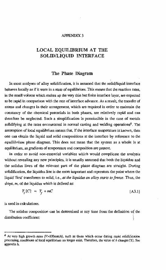
APPENDIX 3
LOCAL EQUILIBRIUM AT THE SOLID/LIQUID INTERFACE
The Phase Diagram
In most analyses of alloy solidification, it is assumed that the solid/liquid interface
behaves locally as if it were in a state of equilibrium. This means that the reaction rates,
in the small volume which makes up the very thin but finite interface layer, are expected
to be rapid in comparison with the rate of interface advance. As a result, the transfer of
atoms and changes in their arrangement, which are required in order to maintain the
constancy of the chemical potentials in both phases, are relatively rapid and can
therefore be neglected. Such a simplification is permissible in the case of metals
solidifying at the rates encountered in normal casting and welding operations#. The
assumption of local equilibrium means that, if the interface temperature is known, then
one can obtain the liquid and solid compositions at the interface by reference to the
equilibrium phase diagram. This does not mean that the system as a whole is at
equilibrium, as gradients of temperature and composition are present.
In order to avoid non-essential variables which would complicate the analysis
without revealing any new principles, it is usually assumed that both the liquidus and
the solidus lines of the relevant part of the phase diagram are straight. During
solidification, the liquidus line is the more important and represents the point where the
liquid 'first' transforms to solid, i.e., at the liquidus an alloy starts to freeze. Thus, the
slope, m, of the liquidus which is defined as:
Τ [C] = Tf + mC
[Α3.1]
is used in calculations.
The solidus composition can be determined at any time from the definition of the
distribution coefficient:
At very high growth rates (V>1(mmm/s), such as those which occur during rapid solidification processing, conditions of local equilibrium no longer exist. Therefore, the value of k changes [1]. See appendix 6.

200 Fundamentals of Solidification
Figure Α3.1
k = CS [Α3.2]
The constants, m and k, are always defined in the present book in such a way that
the product, m(k-1) is positive. In general, m can be positive or negative and k can be
greater or less than unity, respectively.
Two important properties characterise the range of coexistence of solid and liquid for
a given alloy:
∆Το = — m∆Co
∆Cο — Co (1—k)
[Α3.3]
[Α3.4]
All of these properties depend upon the Gibbs free energy (free enthalpy) of the alloy
system, as shown by figure A3.1. The latter relates a free-enthalpy versus
Ι

J ncal Equilibrium at the Solid/Liqud Interface 201
concentration diagram and a free-enthalpy versus temperature diagram to a temperature
versus concentration (phase) diagram. The form of the curves in the ∆G—C diagram can
be described by using the regular solution model [2 - 4] which shows that for, Χ, the
mole fraction of solute B:
Gm =(l—X)G +XGB +ΩΧ(1—X )+RT[Xln(X)+(1—X )ln(1—Χ)] [Α3.5]
where Ω is the interaction parameter.
The curves in the ∆G—Τ diagram depend upon the standard values for the pure
components:
G' = li — TS'
where the dots indicate values for the pure component.
The free enthalpy (Gibbs free energy) difference which exists between the pure
liquid and pure solid is:
∆G = ∆Η' — T ∆,S [Α3.6]
where
Tt
∆Η' = ∆Η; — f ∆c dΤ Τ
θS = ∆Sf — Jψ)dΤ r
and ∆c' = c1 — cs.
The quantity, ∆G°, in equation Α3.6 is very important with regard to nucleation and
growth processes and can be evaluated when the temperature dependence of ∆c` is
known. At high temperatures, the difference in specific heat of the liquid and solid can
be described by:
∆ι = Κ1 Τ + Κ2
For an undercooled melt, ∆Τ =— T f— Τ and [5]:
Ι∆G Ι - ∆Ηf∆Τ ∆ΤΖ[Κ1 + Κ2
ΤΙ 2 Tf + Τ
[Α3.7]
[Α3.8]

202 Fundamentals of Solidification
If the value of ∆c® is unknown, the simplest assumption (and one which is quite
reasonable for metals) is that ∆c = Ο. This leads to:
Ι∆G Ι = ∆ΗT Τ = ∆Sf θΤ [Α3.9]
The quantity, ∆S f , is the difference in slope of the G—T function of two phases
(Fig. Α3.1). For a more detailed discussion of this problem the reader is referred to
reference 6.
From equations Α3.5 and Α3.9, one can now see which parameters influence the
magnitudes of m and k. These are the interaction parameter, Ω, for the atoms of both
species in the alloy, which determines the form of the Gm —X curves, and the melting
entropy, ∆Sf, which separates the origins of the ∆Gm Χ curves. A description of
further relationships between k, m, and the thermodynamic properties is given by
Flemings [7]. For small concentrations of an alloying element, and assuming ideal solution
behaviour, a useful relationship between the melting entropy of the solvent, (A) and the
liquidus slope and distribution coefficient of the solute (B) can be obtained. Under these
assumptions, the chemical potential of the solvent is:
µ; = µ; • + RTIn(1 — Χ )
[Α3.10]
= µΑ + RTln(l —X,)
where Χ and Χ1 are the mole fractions of B atoms in the solid and liquid, respectively.
At equilibrium (j sA = µ )):
∆GA = µq — µA. = RΤln[ Ι 1 —Xl
From equation Α3.9, one obtains:
∆S∆Τ _ 1— Χ RT ~~ 1
[Α3.12]
For small solute concentrations and noting that, for z — 1, ln(z) is approximately equal
to z — 1, it can be seen that the RHS of equation Α3.12 becomes approximately equal
to Xi — Χ. = Χ j(1 — k) when Χ approaches unity. Therefore:
[Α3.11 ]

C ~
Cs e,
e c s L
Local Equilibrium at the SoliWLiquid Interface 203
∆S ∆Τ = 1- k RT Χ1
and substituting for ∆T/Χ1 = m0; the liquidus slope expressed as degrees per atomic
fraction, one obtains:
[Α3.13] ma RT
Or, as Χ1 tends to zero and Τ tends to T f:
1—k = ma RTf
Here, ∆S f. is the melting entropy of the pure solvent of melting point, Tf, and both m
and k have to be defined in terms of mole (atom) fractions.
Figure Α3.2
[Α3.14]

204 Fundamentals of Solidification
Capillarity Effects [8,9]
The total Gibbs free energy of a small solid particle in a melt is inversely proportional
to its size. Because the free enthalpy of the solid increases with decreasing diameter,
while the free enthalpy of the liquid remains constant (if the amount of liquid is much
greater than the amount of solid), the melting point decreases for the pure solid as well
as for the alloy (Fig. Α3.2). The increase in the free enthalpy of the particle, due to its
curved surface (of radius, r), can be regarded as being an increase in internal pressure
(the dot suffix will be dropped for the remainder of this appendix):
∆G = m ∆P [Α3.15]
where Vm is the molar volume (assumed to be constant), and ∆Ρ is given by the specific
interface energy and the curvature:
∆Ρ = σΚ [Α3.16]
Combining equations Α3.9, Α3.15, and Α3.16 leads to a relationship between the
equilibrium temperature drop and the curvature:
Τ - Τ' = ∆7 = ΓΚ [Α3.17]
and
_ σνm ® ~ Γ ∆Sf ~f
[Α3.18]
where ∆Sf is the absolute value of the molar freezing entropy and ∆sfis the volumic
freezing entropy. In order to use these equations, the parameters σ and Κ have to be
defined:
Specific Interface Energy, σ : it is assumed that the solid/liquid interface (in
fact a volume) is a surface across which the properties change discontinuously. The
specific surface energy is defined there as being the reversible work, dw, which is
required in order to create new surface area, dA. In the case of a solid/liquid interface,
the specific interface energy can be set equal to the interfacial tension, Ύ. According to
figure Α3.3, the work necessary to extend the surface by dz is:
dw = fdz = σΙdτ = σdΑ
from which one can obtain the definition:
σ = dw' [Α3.19]

Local Equilibrium at the Solid/Liquid Interface 205
dz
Figure Α3.3
Curvature, K: in two dimensions, the curvature of a function is defined as the
change in the slope, 58, of that function over a length of arc, 51 (Fig. Α3.4a):
χ = δθ Si
and, since 81= r88,
χ = 1 r
More generally, it can be shown that the curvature at a point (61-3. 0) is given, in
Cartesian coordinates, by:
z „ [Α3.20] [1 +
where z and z" are the first and second derivatives, respectively, of the function, z(y).
The average curvature of an arbitrary line segment depends only upon the gradients
of the curve at its end-points, and upon the distance between the latter (Fig. Α3.5). In
the case of surfaces in three dimensions, the curvature can be defined as the variation in
surface area divided by the corresponding variation in volume:
χ = dA dv
[Α3.21 ]
For a general surface with constant principal radii (minimum and maximum at 90° to
each other - Fig. Α3.4b) one can define (for small angles):
I t = r1 8
12 = r2 8
Increasing the radii by dr gives:

206 Fimdameiilals of Solidification
b
Figure Α3.4
dA = 11d12 +12d11 = r1 θdrθ + r2θdrθ
dA = (r1 + r2 )drθ2
dv = 1112dr = (r1 θ)(r2 θ)dr
dv = rlr2drθ2
Therefore from equations Α3.21, Α3.22, and Α3.23,
Κ = (1±1) ?Ι r
[Α3.22]
[Α3.23]
[Α3.24]
In the case of a sphere, r1 = r2 = r so that K = 2/r. In the case of a cylinder, r1 is infmite and r2 = r so that K = 1/r.

Local Equilibrium at the Solid/Liquid Interface 207
Figure Α3.5
Thus, using equation Α3.17, the decrease in melting point due to the curvature of a
spherical crystal in a melt can be written:
∆Ι' = 2Γ r r
[Α3.25]
It is supposed in the above calculations that the value of pis isotropic. The effect of
anisotropy is treated by Aaronson [10].
Mechanical Equilibrium at the Three-Phase Junction
A junction between two solid phases at the solid/liquid interface will form a groove.
At this point, the surface forces will tend to impose an equilibrium (minimum energy)
morphology in which:
f = 0
From figure Α3.6, it is evident that this condition will be satisfied when:
άρ = αι c cos(81 ) + σ 1 cos(82 )
and [Α3.26]
a1 sίn(Θ1) = ο-
sίn(Θ2 )
In establishing mechanical equilibrium, it is important to consider the equilibrium of
the moments acting on the junction (second equation above) since this affects the angle

208 Fundamentals of Solidification
Figure Α3.6
of eutectic interfaces or grain boundaries with respect to the solid/liquid interface. In
most cases, the angle is expected to be close to 900.
Calculation of f(0) for Heterogeneous Nucleation [4]
The application of equations Α3.26 to heterogeneous nucleation shows that true
mechanical equilibrium (Fig. Α3.7b) cannot be established, and that a surface stress
will be set up (Fig. Α3.7a). Due to the presence of foreign crystalline surfaces
(crucible, surface oxide, inclusions) in a melt, nucleation may become much easier. The
effect of these interfaces can be deduced from the energy balance:
∆Gi = (interface energy creation due to nucleation) - (interface energy
gained due to the substrate)
∆G = (Α~~ σε + Αεs σs ) — Αcs σs
∆G = ~kσiε + πΡR2(qs — ~s )
σs = σs + σε εοs ®
θG ε = Αlεσ — πR2 cοs θ σε
θG = ∆G + ∆G = έ ∆g + [Α'— nR 2 cos ® ] σε
[Α3.28]
[Α3.29]
[Α3.27]

Local Equilibrium at the Solid/Liquid Interface 209
ν irr3
Γ 2— 'cos Θ + cos3 Θ] c 3
where:
Α1 = 2πr2[1— cos 8 ]
R = rsin θ
sin2 8= 1 — cos2 θ
dG = (4πr3∆g + 4πr2σιε )[2 — 3cos Θ+ cos3 8
3 4
∆Ghet = ∆Ghom .f(8)
f(θ) 2— 3cos B+ cos3 8 = [ 2+ cos Θ ][ 1— cos 8]2 4 4
[Α3.30]
crystal nucleus
liquid nucleating
2 R particle, substrate
Figure Α3.7

210 Fundamentals of Solidification
References
[1] M.J.Aziz, Journal of Applied Physics 53 (1982) 1158. K.Jackson, G.H.Gilmer,
H.J.Leamy, in Laser and Electron Beam Processing of Materials (C.W.White,
P.S.Peercy, Eds.), Academic Press, New York, 1980, p. 104. R.F.Wood,
Physical Review Β25 (1982) 2786.
[2] D.R.Gaskell, introduction to Metallurgical Thermodynamics, McGraw-Hill,
New York, 1981.
[3] M.Hillert, in Lectures on the Theory of Phase Transformations, (H.I.Aaronson,
Ed.) Transactions of the Metallurgical Society of ΑΙΜΕ, New York, 1975, p. 1.
[4] J.S.Kirkaldy, in Energetics in Metallurgical Phenomena, Volume IV
(W.M.Mueller, Ed.), Gordon & Breach, New York, 1968, p. 197.
[5] C.V.Thompson, F.Spaepen, Acta Metallurgica 27 (1979) 1855.
[6] K.S.Dubey, P. Ramachandrarao, Acta Metallurgica 32 (1984) 91.
[7] M.C.Flemings, Solid Wcation Processing, McGraw-Hill, New York, 1974.
[8] W.W.Mullins, in Metal Surfaces - Structure, Energetics, Kinetics, American
Society for Metals, Metals Park, 1963, p. 17.
[9] R.Trivedi, in Lectures on the Theory of Phase Transformations, (H.I.Aaronson,
Ed.) Transactions of the Metallurgical Society of AIMS, New York, 1975,
p. 51.
[10] H.I.Aaronson, in Lectures on the Theory of Phase Transformations,
(H.I.Aaronson, Ed.) Transactions of the Metallurgical Society of AIMS,
New York, 1975, p. 158.

APPENDIX 4
NUCLEATION KINETICS IN A PURE SUBSTANCE
In order to determine the nucleation rate, it is necessary to determine the number of
critical nuclei and the rate of arrival of atoms necessary to make up these nuclei [1 - 3].
Equilibrium Distribution of Nuclei in an Undercooled Melt
The system shown in figure Α4.1 represents a mixture of N' atoms in the liquid state
and Ν„ small crystal clusters, each of which contains n atoms. The free enthalpy change
of such a system when compared with another one, at the same temperature, which
contains only atoms and no crystal nuclei is:
∆G = Ν. ∆G - Τ∆S~ [Α4.1]
Here, ∆G„ is the free enthalpy change due to the formation of one nucleus containing n atoms and ∆S„ is the entropy of mixing of Ν„ clusters with Nj atoms. (In this
equation, the existence of an ideal mixture of crystal clusters and atoms of liquid is
assumed. Therefore, the mixing enthalpy, ∆Η„, is equal to zero.)
In the case of sub-critical clusters (known as embryos), ∆G„ is positive due to the
work of interface creation. This is demonstrated in figure Α4.2 and corresponds to
figure 2.2 where n and r, characterising the difference in size, are related by
crystal cluster
atoms of liquid
-
10nm
Figure Α4.1

212 Fundamentals of Solidification
n
Figure Α4.2
equation 2.2. The value of ∆G can be determined in an analogous manner by using
equation 2.3, and leads to the relationship:
∆G = η∆G' + Α σ n n
Α = nn2/3
where ∆G is the atomic free energy difference, Α is the interface area of the cluster, η is a form-factor which depends upon the shape of the cluster, and n113 is proportional to the cluster diameter.
The mixing entropy of equation Α4.1 can be derived by using the well-known
relationship:
∆S = 1ι81n[ N1 i Νi )!1
Ν.Ν. [Α4.3]
and therefore
∆G = Ν ∆G — !ιB Τ1η[(Ν + Ν )!] + k Tln[N!] + k Τ1η[Ν !] [Α4.4]
where ∆G is always positive for critical nuclei. An increase in ΝΝ will first decrease
the total free energy of the system, due to the mixing of clusters and atoms (Fig. Α4.3), and then reach a minimum value which represents the equilibrium concentration of
[Α4.2]

Nucleation Kinetics in a Pure Substance 213
clusters for a given undercooling. Applying Stirling's approximation for large values of
N, i.e. ln(N!) = Nln(N) — N, differentiating equation Α4.4 with respect to Νη, and
setting the result equal to zero gives:
= 0
from which:
Ν„ ∆ exp[— [Α4.5]
Ν1 + Ν
Since Ν1» Ν„
Νι = eXp[ 4.ι
The number of nuclei (critical clusters) in equilibrium is therefore:
Ν0 = 117exp[ ∆G„ ]
kB T [Α4.6]
where ∆Gn is the energy barrier for nucleation as defined in figure Α4.2. These
relationships are given in figure 2.3 of the main text.
c9 ®
1 equilibrium
Nn number of cluster
Figure Α4.3

214 Fundamentals of Solidification
ΙΖ1- a of Formation of Stable Nuclei
The nucleation rate must be proportional to the number of crystals of critical size,
Ν . However, in order for these crystals to grow, the addition of further atoms is
required. The system, containing clusters of size, n°, is in an unstable state and can
produce smaller or larger clusters (Fig. Α4.2) in order to decrease its energy.
Therefore, it is necessary to determine the rate of incorporation, dn/dt, of new atoms
into the nuclei. The nucleation rate is then:
Ι = Ν° ±L
[Α4.7]
where the adsorption rate, dnldt, is the product of an adsorption frequency, v, and the
density of sites at which the atoms can be adsorbed by the critical nucleus, n:
do = vn° dt S
The adsorption frequency is:
∆Gd ν = óexpL—~Τ ]ρ
where ν0 is the atomic vibration frequency, exp[—∆Gd/kΒT] is the fraction of atoms in
the liquid which are sufficiently activated to surmount the interface addition activation
energy, ∆Gd, and p is the adsorption probability.
The site density is given by:
n° = A°n S η ε [Α4.9]
where Α° is the surface area of the critical nucleus and nc is the capture site density per
unit area.
The nucleation rate is therefore:
and
θG,° + ∆Gd Ι = Ioexp~
keT ]
Ιο = Νt • vcρΑ~°n
[Α4.10]
Since the exponential term is extremely sensitive to small variations in the argument
(Fig. 2.5), the exact value of ί is relatively unimportant and, for metals, is often
approximated by:
[Α4.8]

Nucleation Kinetics in a Pure Substance 215
lη = Ν T Ι ~~.) = Ιί • π = 1042/m3s [Α4.11]
All of these relations assume the existence of a steady state and are not of general
applicability. Nevertheless, they give a good guide to the principles which are involved.
For a more complete treatment of nucleation theory, the reader should consult
reference 3. In the case of alloys, the present approach has to be modified [4].
References
[1] D.Turnbull, J.C.Fisher, Journal of Chemical Physics 17 (1949) 71.
[2] D.R.Uhlmann, E.Chalmers, Industrial and Engineering Chemistry 57 (1965) 19.
[3] J.W.Christian, The Theory of Transformations in Metals and Alloys (2nd
edition), Pergamon Press, Oxford, 1975.
[4] C.V.Thompson, F.Spaepen, Acta ldietallurgica 31 (1983) 2021.

Activation energy
for departure for an atom of site n=3
n = 1 —
α
3
APPENDIX 5
ATOMIC STRUCTURE OF THE SOLID/LIQUID INTERFACE
In order to explain the principles involved, the simple case of a two-dimensional
crystal consisting of 'square atoms' of only one type, which interact only with their
nearest neighbours and form single-layer interfaces, will be treated here. It is assumed
that there are three different structural elements making up the surface structure (three-
site model - Fig. A5.1). This situation has been treated in detail by Jackson [1]. The
model is an improved version of a previous one which was developed by the same
author [2].
There is a continuous interchange of sites due to the thermally activated adsorption or
desorption of atoms. For example, an n = 1 site will be transformed into an n = 2 site
by adsorption of one neighbouring atom. It is assumed that, after a short time, the
interface structure reaches a steady state, i.e., the overall density of the three types of
site does not change with time. The rate of adsorption of atoms is independent of the
rate of departure. Both are activated processes which are similar to diffusion in the
liquid, but the desorption of atoms is more difficult from an undercooled crystal, due to
Figure Α5.1

Atomic Structure of the Solid/Liquid Interfere 217
the gain in energy which occurs when an atom is added to the solid/liquid interface. The
probability of adsorption will depend upon the roughness of the interface; the greater the
density of steps (and therefore the greater the number of exposed atomic bonds
presented to the liquid), the higher is the probability that an atom will be incorporated
into the crystal; as a result of the stronger bonding involved.
The rate of atom arrival, J±, is governed by:
+ = Jóexp[—RT]
[Α5.1]
where Q is the activation energy for diffusion in the liquid. The flux of atoms leaving is
determined by:
• = Jo - exp[— RT]exp[ 2n∆Ιί
f ] zRT [Α5.2]
where tff is the latent heat of fusion, n is the number of bonds which have to be
broken by an atom in leaving the crystal, and z is the coordination number (4 in the case
of a two-dimensional crystal). An atom which makes two bonds with the crystal (i.e.
half of the maximum possible number of bonds) can be viewed as being half in the solid
and half in the liquid. At the melting point, Tf, the rates of arrival and departure from
such sites (n = 2) should be equal. Thus,
Jóexp[—RT ]
Jo exp[— RT
]exp[—~] f f
[Α5.3]
Therefore:
Jo = exp[R• ] j
Combining equations Α5.2 and Α5.4, and rearranging the exponential terms:
J = Jóeχρ[—RQ
]exp[RT 2L]
The second exponential term can be regarded as being a measure of the probability that
an atom which has n neighbours will leave the site, that is:
04) [ 2RΤ
The net flux is determined by the difference between equations Α5.1 and Α5.5:
[Α5.4]
[Α5.5]

218 Fundamentals of Solidillcation
Figure Α5.2
J = Jήexp[— RT 1[1— Ρα ]
It is now possible to set up balance equations for the arrival and departure of atoms at
various types of site. The detailed calculations have been given by Jackson [1].
Carrying these through and realising that, if (∆ΗJ/RΤf)(∆Τ/Τ) < 1,
r H ∆Τ η _ ∆Η ∆Τ eXP[ R7 Τ J ι RΤf Τ
the net growth rate, V. of the crystal becomes:
V = Jv' = v'JJ exρ[— RΤ]α( ~T )f[hk] [Α5.7]
where α = ∆H f/RΤf = ∆S/R (the dimensionless melting entropy) and V is the atomic
volume.
Therefore, to a first approximation, the growth rate is a linear function of the
undercooling. It also depends upon the magnitude of the crystallographic factor, f[hk],
which is a function of the interface structure. It thus depends upon the value of a and
upon the Miller indices, (hk), of the crystallographic plane. When a takes on high
values (e.g. 10), the fraction of extra atoms or holes in the interface is proportional to
exp[—a].
For (11)-faces of the present square crystal (Fig. Α5.2), f is independent of a but
this is not so for the (10)-face (table A5.1). The reason for this is that a 45° edge
[Α5.6]

Atomic Structure of the Solid/Liquid Interface 219
Figure Α5.3
exhibits many growth steps, which cannot be removed by atom addition. When the
value of a is large, the (11)-edges will grow much more quickly and leave the crystal
bounded by slow-growing (10)-edges (Fig. Α5.3 - see also Fig. 2.9). Note also in
table Α5.1 that, for small values of a, the growth is almost isotropic (f[10] J[11]).
This behaviour is typical of metals.
Table Α5.1 Crystallographic Factor, f[hk], of two Faces of a Square Crystal
a f[10] f[11]
1 0.56 0.60
5 0.30 0.60
10 0.039 0.60
References
[1] K.A.Jackson, Journal of Crystal Growth 3/4 (1968) 507.
[2] K.A.Jackson, in Liquid Metals and Solidification, American Society for Metals,
Cleveland, 1958, p. 174.

APPENDIX 6
THERMODYNAMICS OF RAPID SOLIDIFICATION
Interface Kinetics
As e,cρlaiηed in appendix 3, under normal solidification conditions the non-faceted
solid/liquid interface itself is close to equilibrium even if concentration and temperature
gradients exist in the adjacent phases. Therefore, the assumption of local equilibrium is
useful when the short-range diffusional rate of atoms crossing the interface is much
higher than the rate of arrangement of atoms into a configuration of low mobility (e.g.
crystallisation).
Consider the case of an alloy, and assume now that the time required to freeze-in
solute atoms is, due to rapid interface movement, much smaller than the time taken to
diffuse through a characteristic distance, Si, which is of the order of the interatomic
distance (Fig. Α6.1). As a result, solute is incorporated into the solid at a concentration
which is different to the equilibrium concentration. Such solute trapping will always
occur, at least partially, if the following condition is satisfied:
= δ.I /V <_ δ2/D. [Α6.1]
where Di is the interface diffusion coefficient. From this relationship, one can also see
S .--. δ;
Figure Α6.1

∆µe
τ
0 χ
Thermodynamics of Rapid Solidification 221
Χ 0
Figure Α6.2
that local equilibrium will be lost when the interface Pdclet number, Ρί (= δίν/D ς) satisfies:
Ρ >_ 1 [Α6.2]
At very high interface Ρέclet numbers, k,, is equal to unity (see below). In order that
this should occur, another condition must be satisfied. This is that the change in free
energy must still be negative (at least slightly) when the liquid transforms to a solid.
This is best seen with the aid of free energy diagrams (Fig. Α6.2).
Το - Condition
For a given interface temperature, T' = Τ between solid (a) and liquid (1) the
equilibrium compositions are X ά and X j. Now, if the interface composition is Χι and
k„ = 1, solid a of the same composition as the liquid, Χ1 , cannot form since its free
energy is higher than that of the liquid phase. However, solid of composition, Χα, can
form from liquid of composition, Χ1 , at Τ since its free energy will decrease. The
range of compositions of a which can crystallise from liquid of composition, Χ1 , at Τ
χ°

222 Fundamentals of Solidification
is given by the inter°section of the tangent at G(Χ) with the curve, Ga,.
In order to trap solute completely (k,, = 1) at T1= T', the composition must become
equal to, or smaller than, Χ0. That is, the maximum solid composition at T
corresponds to Χ0 (= Χ1 = Χα) and T = Ρ0. Following the approach of Baker and Cahn [1] and Boettinger and Coriell [2], one
can now calculate the driving force for crystallisation as a function of k,,. This tends
towards unity when V becomes very large. From the definition of the chemical
potential, one can write for solute B:
µΒα = σα + RT1n[a] α = µΒι + RT1n[αι ]
where the activity, a, of the solute equals VX. Since, for simplicity, only dilute
solutions will be considered here one can assume that the activity coefficient, y, is
constant. ,
From the condition of equilibrium, one has:
µΒα + RTln[γΧe ] = oI α α + RTIn[yXle ] [Α6.4]
and, under non-equilibrium conditions,
µΒα + RTIn[γα Χα ] = µ8Ι + RTIn[γΧl ] + ∆µ8 [Α6.5]
From equations Α6.4 and Α6.5, one deduces that:
44B = RTIn[k /k ] [Α6.6]
where the non-equilibrium distribution coefficient, kv, is equal to Χα /x1, and the
equilibrium distribution coefficient, k, is equal to Χα ΙΧel' The same calculation can be carried out for the solute, A, in a binary system of
concentration, (1 — Χ). From the relationship:
∆G =
it follows that:
∆G RT
— [1—k Χl]1η[11 χΧ1 1- kXΙ, + kXt ln[~]
and one obtains for Xi = X, in the case of dilute solutions (Χ1 < 1) and after
approximating ln[z] (when z —i 1) by z —1,
[Α6.3]
[Α6.7]
[Α6.8]

Tbemrndymimics of Rapid SolidifIcation 223
∆G (1— kvXι)Xι(k— k,) + kΧι 1η[~] RT 1 — kΧι k [Α6.9]
The first term on the right-hand side of equation Α6.9 is approximately equal to
Χ1[k — k',], and one finally obtains, for the thermodynamic relationship between k, and ∆G (at the interface),
∆G *lRT* = Χι*k — k [1_1n()]) [Α6.10]
Using the relationship, ∆G = ∆S/ΙT, one can relate the interface undercooling to the
deviation from local equilibrium, as expressed by k,.
Α further undercooling is associated with the kinetics of rearrangement of the atoms
at the interface (Fig. Α6.1). This value can be obtained using:
∆Gk = ∆Sf ∆Τk
where ∆Sf = RTf(1 — k)/m (see equation Α3.14). This gives, for the kinetic driving
force:
∆Gk /R f = [(1—k)/m](f +m —7)
Adding equations A6.10 and Α6.11'one finds, for small undercoolings, T*—Tf:
∆G/RT = [(1-k)/m](Tt. +m) *-T)+ Χ1*k -k [1—ln( )]
[Α6.11]
[Α6.12]
From the relationship between ∆G and the growth rate [3],
V = f Vo [ 1— exp(∆G/RT* )] [Α6.13]
where f is the fraction of interface sites which are growth sites (close to unity for
metals), and V0 is the upper limit of interface advance (comparable to the velocity of
sound). Since V « νθ, one can write:
* V/V0 = - ∆G/RT
[Α6.14]
and, combining equations Α6.12 and Α6.14, one obtains for the temperature of a:planar
interface:
Τ = + + [m)4*/(Ι — k)]tk — k [1 — Ιn[]] )± (V/V0 )[m/(l — k)]
[Α6.15]
and, for a dendrite tip of radius, R:

224 Fundamentals of Solidification
Τ = Tf — 2Γ/R + mJf • [1 + f(k)] + (VN0 )[ml(1 —k)] [Α6.16]
where f(k) = (k — k„[1 — ln(kν/k)] )/(1 — k) and the kinetic liquidus slope is
m' = m[l + f(k)].
Setting R = φΡ in equation A6.16, V0 =00 (infinitely rapid interface kinetics), and
k', = 1, one obtains the equation fιir the To-line:
Χl m ln(k ) T0 = Tf + k — 1 [Α6.17]
Because of the simplifications made, this equation holds only for dilute solutions.
Non-Equilibrium Distribution Coefficient
The last equation to be developed is that which describes the relationship between the
non-equilibrium distribution coefficient and the rate of interface movement. This can be
easily found by considering the two extreme cases shown in figure 7.1. At V = 0, the
interface is at equilibrium: µ a = µ1 and k,, = k. Here, the net flux of atoms crossing the
interface is zero. The other extreme case, V = φΡ, leads to complete solute trapping and
k = 1 (Χ a = Χ 1 ). This sets up a gradient of chemical potential which tends to drive
atoms from α to 1. This flux is proportional to the chemical potential gradient:
Jd = — Χ (dµ/dz) [Α6.18]
For dilute solutions, the interface diffusion coefficient is related to the interface
mobility, M1, via:
giving:
D. = M. R Τ
ι ι [A6.19]
Jd = — (D. Χ /RΤ)(dµ/dz) [Α6.20]
Note that the interface diffusion coefficient can be substantially lower than the bulk
liquid diffusion coefficient. The chemical potential gradient at the interface, in the case
of dilute solutions (see equation Α6.6), is:
(dµ/dz) _ (∆µe /δ1) = RΤ ln(k /k)/δ [Α6.21]
Setting the composition of the interface, Χ, equal to its mean value, (X! + Χ a )/2 =
Χ 1(1 + k,,)/2 leads to:

Thermodynamics of Rapid Solidification 225
Jd = — (D /2δ.)Χ1 (1 + k ) ln(k', /k) [Α6.22]
This flux in the growth direction, which arises from the chemical potential gradient,
must be equal to a source term if steady-state conditions are to prevail at the interface.
This source term is simply the solute rejected at the interface:
J = VΧi (1—k)
Setting Jd equal to Jr , one obtains:
Vδ /q = (1/2)[(1 + k )/(1 — k )] 1η(k /k)
[Α6.23]
[Α6.24]
This is just one relationship between the interface P6clet number (Pi = νδj/D~) and
the non-equilibrium distribution coefficient. Others have been derived by Aziz [4]. For
example, again for dilute solutions:
k = (k + Ρ )/(1 + Ρ ) [Α6.25]
The general form of all of these relationships is such that kv = k when Ρί is much
smaller than unity, and k„ = 1 when Pί is much greater than unity (Fig. 7.3). The
critical growth rate at which kv changes markedly depends mainly upon the interface
diffusion rate, Di /4~. This is of the order of 0.1 tό 1 m/s.
References
[1] J.C.Baker, J.W.Cahn, in Solidification, ASM, Metals Park, Ohio, 1971, p. 23.
[2] W.J.Boettinger, S.R.Coriell, in Science and Technology of the Undercooled Melt
(P.R.S ahm, H.Jones, C.M.Adam, Eds.), Martinus Nijhoff Publications,
Dordrecht, 1986, p. 81.
[3] D.Turnbull, Journal of Physical Chemistry 66 (1962) 609.
[4] M.J.Aziz, Journal of Applied Physics 53 (1982) 1158.

APPENDIX 7
INTERFACE+ STABILITY ANALYSIS
The constitutional undercooling criterion provides a useful means for estimating
whether a solid/liquid interface will he planar under directional solidification conditions.
However, from a theoretical point of view it has several faults. Firstly, it does not take
account of the effect of surface tension. It is expected that this will tend to inhibit the
formation of perturbations. Secondly, it takes account only of the temperature gradient
in the liquid. Thirdly, the constitutional undercooling theory does not give any
indication of the scale of the perturbations which will develop if an interface becomes
unstable. In order to deduce more information about the morphological instability of a
plane interface than that provided by the constitutional undercooling theory, one must
suppose that the interface has already been slightly disturbed and then ask whether the
disturbance will grow or disappear (chapter 3). To this end, it is sufficient to consider a
sinusoidal interface form having a very small, time-dependent amplitude (Fig. Α7.1). (Provided that the amplitude is small, a sinusoidal form represents the most general
disturbance possible; it can be supposed to be one term of the Fourier series describing
any possible disturbance.)
The object of the present calculations is to determine the conditions which govern the
growth or decay of a perturbation at the solid/liquid interface (Fig. 3.1). In order that
the results should be applicable to high rates of solidification, it is necessary to consider
both solute and heat diffusion. In the case of solute diffusion, the solid phase can be
neglected because the rate of diffusion in the solid is so slow. In the case of heat
diffusion, both the liquid and solid phases have to be considered. The reader is advised
to consult the section on the 'slightly perturbed interface' in appendix 2. The latter
λ
z = E Sin wy
Figure Al.!

Interface Stability Analysis 227
section introduces, in the context of a simpler problem, all of the techniques which will
be used below.
Three equations have to be solved. These are, for two-dimensional diffusion:
ιd2C + d2C +VdC = dy 2 az 2 D λτ
which describes the solute distribution in the liquid,
ι32Tς ά2Τ µ ~ 2 z λτ =0
ι3y λτ αι
which describes the temperature distribution in the liquid, and
á27s d2!s V dΤs 2 + zz +adz
=0 d ,,
[Α7. la]
[Α7.1 b]
[Α7.1c]
which describes the temperature distribution in the solid. Here, V is the growth rate and
D, aj, and a, are solute and thermal (liquid and solid) diffusivities respectively.
For a plane interface, suitable solutions to these equations are, respectively:
C = Co — 2 ~ eXp[— Dz ]
= Τ0 + G1a'
expl— áz ι
Τ = Το + Gvαs[1— áz
']
S
[Α7.2α]
[Α7.2b]
[Α7.2c]
where Gc, G1, and Gs are solute and temperature gradients (liquid and solid)
respectively at the plane interface. Note that Co is the concentration at infinity, but Τ0 is
the temperature at the interface. As in appendix 2, the plane interface is assumed to be
perturbed so that it has the form shown in figure Α7.1. According to perturbation theory
(appendix 2), the solute and temperature distributions can be assumed to be of the form:
C = C0 — GV exp (_ - ) + Aεsinωy exp(—b z )
Τ= Το + GV ι[1—exρ(— a
z)] + Βεsίπ ωy exp(—bι z) ι

228 Fundamentals of Solidification
Τ = Τc + Gv S [1—exp(— áz)] + Rεsinωyexp(—b z) S
[Ά7.3c]
where A, B, R, b, b1, and bs have to be determined by applying the various physical
constraints which are imposed by the situation:
Each of the b-values can be found by inserting the derivatives of the relevant
equation into the corresponding differential equation (Α7.1). In this way (appendix 2),
it is found that:
b = 2v~D +
[(~)2 + ά ]ι/τ
ε
b = ~ + [( V )2 )2 + ώ l 1/2
1 [ J
b = ---- -- · '
l~,2+ά]
S
S
1/2
[Α7.4α]
[Α7.4b]
[Α7.4c]
The value of R can be found by recalling that, at the perturbed interface, the
temperatures in the solid and in the liquid must be the same. That is (putting S =
ε sinwy = z as in appendix 2):
Το + Gya1[ 1—exp(— as)Ι +BSexp(—b S) =
= Τ0 ± ί s[Ι eΧρ( as)]+RSexp(—bS) S
Since ε is very small, one can write exp(—ε sinwy) 1.— ε sinwy, and terms in ε2
disappear. This leads to:
R = (GI —G)+B [Α7.5]
Α second condition is imposed by the coupling of the absolute temperatures and
concentrations at the interface. That is, the actual temperature at the perturbed interface
must correspond to that which is given by the sum of the constitutional supercooling
and capillarity effects if the attachment kinetics are very rapid. This can be written:
Τ+ = Tf + mC+ — Γω2S
[Α7.6]
where the index, +, indicates a value determined at the perturbed interface, and Tf is the
melting point of the pure substance. The last term on the RHS involves just the second

Iiiterfxc Stability Analysis 229
differential of the perturbing function rather than the full curvature expression, Κ = z"/(1+i 2)l/2. This is permissible because of the smallness of ε. Thus:
Τo + GVaI [1—exp(— aS
)] + ΒSexp(—b1S) = ι
= Tf + m [Co — DV exp(— - ) + AS — exp(—b S )J — Γω2S
That is:
Το + G1S + BS = Tf + mCe — rnDG + mG S+ mAS — Γω2S
Since, for the perturbed interface, Τρ = Τf+ mCo — mDGc/V, one can write:
G,S + BS = mGS + mAS — Γω2S
Cancelling S throughout leads to:
B = mG + mA — Γω2 — G1
Thus, one now has B in terms of A. In order to eliminate this last remaining
unknown, one imposes the condition that the gradients of solute and temperature must
satisfy solute and heat conservation at the perturbed interface for the same growth rate.
This can be written:
κsG+ — κιG~ DG+ ~f (k-1)C+
[Α7.8]
where κs and lq are the conductivities of solid and liquid, respectively, and ∆hf is the
volumic heat of fusion. The quantities which are marked +, must be evaluated at the
perturbed interface. That is:
G+ = G — GS VS— bRS S s a s
Gl = Gl —Gt VS— b1BS α1
=G —D`VS— bAS
[Α7.9α]
[Ά7.9b]
[Ά7.9c]
[Α7.7]
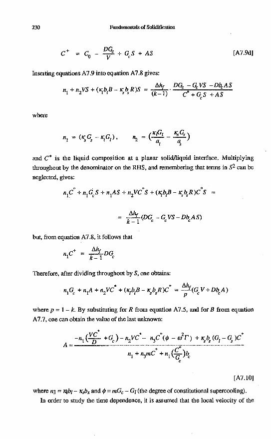
230 Fimdamentais of Solidilbition
C+ =Co — ` +GS +ΑS [Α7.9d]
Inserting equations Α7.9 into equation Α7.8 gives:
n1 +n2VS+ ( bIB — bR)S = ~ DG GVS —DkA S
(k-1) C + GS +AS c
where
η1 = (xG — κGι ), nZ = ( κG11 áGs ) ι s
and C* is the liquid composition at a planar solid/liquid interface. Multiplying
throughout by the denominator on the RHS, and remembering that terms in S2 can be
neglected, gives:
n1C.
+ n1G S+ n1AS + n2VC. S+ (κbιΒ — κ b R )C* S =
_ k-1(DG —GVS—DbAS)
but, from equation Α7.8, it follows that
n1 C+ = k
hf DG
Therefore, after dividing throughout by S, one obtains:
α1G + η1Α + n2VC* +(κbιΒ — κ b R)C« _~(G V+Db A) ρ
where p = 1— k. By substituting for R from equation Α7.5, and for Β from equation
Α7.7, one can obtain the value of the last unknown:
* *
n1 + n3mC* + ε
[Α7.10]
where n3 = ιgb1— ιsbs and φ = mG — Gj (the degree of constitutional supercooling).
In order to study the time dependence, it is assumed that the local velocity of the
—η1( D +G ~ - n2VC*- n3C*(φ — ώ Γ ) + κ b (Gς — G )C Α=

ε ε — n2V + ιctbtB — ις.bs R
∆13. [Α7.14]
Interface Stability Analysis 231
perturbed interface is of the form:
+ έsinωy [Α7.11]
This must be equal to the heat conservation term on the LHS of equation Α7.8. By
inserting the values from equations Α7.9a and Α7.9b, one obtains:
+ έsinωy =
(κG — κGt ) +(Ká t
s )Vesinwy + (κ b Β — K b R )εsinωy 1 s ss
∆hf
or
+ έsίηωy = ηι + n2Vεsinωy + (iqb,B - ιςbR)εsinωy [Α7.12 ∆hf ]
The above equation expresses the identity of two polynomials (in έsinωy).
Therefore, the equivalent coefficients on the two sides must be equal. Thus:
V — >4G~ κtG1 [Α7.13α]
and
n2Vεsinωy + (xtbtB — ιςbR)εsinωy έsίnωy — [Α7.13b]
That is,
The sign of έ/ε determines the stability of the interface. If it is positive for any value
of w, then perturbations with that wave-number will be amplified. In order to study the
stability behaviour in detail, it is necessary to use equations Α7.5 and Α7.7 in order. tο substitute for R and B, respectively, in equation Α7.14. That is:
ε _ n2ν — ις4(G, — Gs)+(κibt — Ksbs)(0 — ω2Γ+ mΑ) ε ∆hf
[Α7.15]

Ga >G,
Ai
α
232 Fundamentals of Solidification
ω λ Ο
— ω
Figure Α7.2
This equation is shown in figure Α7.2 for two temperature gradients (G = Gj = Gs). At
the lower gradient Gl, the function has two zeros; limiting the range of instability to a
band of w. The largest marginally stable w-value defines the smallest λ-value which is
used in dendrite growth theory. The denominator of equation Α7.15, after substituting
for A, will be the same as the denominator of equation Α7.10. Examination of the
denominator shows that it is always positive and therefore cannot affect the stability of
the interface. Therefore, attention will now be restricted to the numerator. This can he
written as:
έ = [nln2V — η1η4 + It tlt3(φ — ω2
Γ)] ( ~ + G ) — nln3lD + ~a Jm ε
where 124 = κsbs (G1 — Gs). Further rearrangement gives the final result for marginal stability, i.e. for έ/ε = 0:
where
— Γώ — [κ'ιGι ξι + κ•G ξs ]+mG ξ C = 0 s
ξι = [b1 — (V lαι)] l[ κtbι + κ sb]
ξs = [b — (Vlα )] l [κ'ιbι + s b ]
ξ~ _ [be— ]/[b ~ ]
[Α7.16]

Interface Stability Analysis 233
= κς/(κ1 + κ )
κ = κ l(κi + κ)
In order to understand the implications of this very important result, it is helpful to
assume, for the moment, that κs = Κι, as = αι, Gs = G1= G, and ξs = ξΡ~ . The latter is
true when w» V/a. (It is also true for the case of constrained growth with G > 0 when Gs = G1.). This corresponds to the small thermal Ρ6clet number solution of
Mullins and Sekerka [1] but allows for large solutal Ρeclet numbers. Under these conditions, equation Α7.16 becomes:
- ω2Γ(b- D ) - G (ba- ) + mG (be- D ) = 0 [Α7.171
Upper Limit of Stability (Absolute Stability)
Writting equation Α7.17 in the form:
-Γω2 -G+mG ξ = 0
and assuming that the Ρέclet number is much larger than one, i.e. ξc -~ π 2/kΡ2, one obtains:
- Γω2 - G+ mG n2/kΡ2 = 0
In most cases, it can be assumed that G can be neglected at very high growth rates, so
that:
- Γω + mG π /kΡ2 =0
Substituting for wand Ρ gives:
- 4π Γ/λ2 + mG (π2/k)(4D2/ν2λ2) = 0
Because it is assumed throughout that the long-range diffusion field is the same as that
for the plane front, one can substitute ∆ΤoV/D for mGC. Thus:
kVΓ/θΤοD = 1
When this condition is satisfied or exceeded, the interface will be stable, regardless
of the value of G, if G << Ga (Fig. 7.5). This is referred to as 'absolute stability'. One

can define a critical velocity for absolute stability:
( á)c ∆T0D
kΓ [Α7.18]
234 Fundamentals of Solidification
Using typical values for metals: ∆Τ0 = 10Κ, D = 5 x 10⁻³mm2/s, k = 0.5, and
Γ = 10-4Κmm, the limit of absolute stability should be attained when V is greater than
lm/s. Such rates are very high but can be obtained in rapid solidification processes such
as laser surface melting. At these rates, account must be taken of the value of the
distribution coefficient, which is a function of the growth rate and may approach unity
(see appendix 6)' .The change in k will decrease (va)c via the decreased ∆Τ0 and
increased k values.
Although the gradient, G', is considered to have a negligible effect in the above case,
it is still positive. One can also consider the case where the temperature gradient in the
solid is equal to zero and the gradient, Gj, in the liquid is negative; as in the case of
equiaxed grain growth. The growth rate is still assumed to be very high. Equation
Α7.16, in the case where Gs = 0 and κs = iq, becomes:
— Γω— 0.5G1 ξ1 +mGξ~ = 0
Substituting the high Ράclet number approximations, ξl = 2π2/Ρ2/ and ξ = π2/kΡ~
gives:
— Γώ — Gl (π2/ή) + mG (π /kP2) = 0
This expression determines the form (values of w) which the perturbed interface
must assume in order to satisfy all of the conditions of the problem.
From the signs of the terms in equation Α7.16, one can immediately deduce the
effects of the parameters involved. For example, increasing ώ2Γ (curvature effect) or G
(imposed temperature gradient) tends to decrease the value of έ/ε and thus increases
the stability, whereas mGc (liquidus temperature gradient) is always positive (since m
and Gc always have the same sign) and therefore decreases stability.
If equation Α7.16 is further simplified by making the assumption that k is equal to
zero (that is, p = 1), one can immediately obtain the result:
ω2 = φ/Γ [Α7.19]
which, as pointed out in section 3.4, is the same as the result derived there using very
Note that the limit in equation Α7.18 can also be derived by assuming that, in equation Α7.17, the value of G becomes irrelevant when the de-stabilizing term, mGc, is balanced by the term, ν2kΓ/D2. Equating the Iwo terms again gives equation Α7.18.

Interface Stability Analysis 235
simple arguments.
Another relatively simple step which one can take is to replace the exact expression
for b (which leads to an intractable cubic equation) by bε —ν/D + (D/V) ω2 (which
implies w << V/2D). This leads to the equation:
DT~ — (φD α )0)2+G ~ = 0
Using Descartes rule of signs, if the equation is to have no positive roots (implying
stability) then the coefficient of ω2 must be negative. This leads to the stability
condition:
G > mG —V 2Γ D [Α7.21 ]
Returning now to consider the full equation (Α7.15), one question of interest is how
ι, ξs and ξc vary as the parameters change. This is most easily seen by again assuming
that a' = as and iq = κs, which is true, for example, in the case of organic materials such
as succinonitrile. This then leads to the equations:
= 1 — (V/2αί) / [(//2(11)2 + 0)2]1/2 [Α7.22α]
ξΡs = 1 + (V/Zαs ) / [(V12a5 )2 + ~2] 1/2 [Α7.22b]
= [1 -(1 + 4D2ω2/ν2)1ή / [1 - 2k— (1 + 4D2ω2/ν2 )112] [Α7.22c]
By substituting the relevant Ράclet numbers, these equations can be written in the
corresponding forms:
ξι = 1
ξs = 1
ξΡ~ = 1
- 1/[1 + (2π/P )2]ι l2
+ 1/[1 + (2π/Ρ )2]ι/2
— 2k/ [1 + (2π/Ι )2] 1/2 — 1 + 2k)
[Α7.23α]
[Α7.23b]
[Α7.23c]
As can be seen in figure Α7.3, all three are equal to unity at low Ρέclet numbers, and the
first and last tend towards zero as the Ρ6clet number tends towards infinity. The second
of the three tends towards 2 as the Ρ6clet number approaches infinity. When the Ρ6clet
number is high but not infinite, the expressions can be further simplified since 1/[1 +
(2π/Ρ)2] 1/2 is approximately equal to 1— 2π2/Ρ2 under these conditions. This gives:
[Α7.20]

236 Fmidamentals of SolidifIcation
Ι
2.0
W
ο
0.1
1.0 10.0
100 Peclet number
Figure Α7.3
ξl = 2π /Ρ2
ξs Ε 2 — 2π lΡ2
Ε π2/kP2
P » 1
Replacing mGc, Pi, ο, and Ρc by their respective definitions gives:
—G át + ∆Τ0D = V 'V2 Tk
For growth in undercooled melts, with Gs = 0, the heat flux balance is V∆hf=— ΙηGι . Therefore:
∆h,αt + ∆ΤοD = V κΤ Tk
or
V _ D∆Το + at~r
Γk Γ
where ®t is the unit thermal undercooling. This condition can be written [2]:
á= ( a )c + ( á ), [Α7.24]
This equation shows that absolute stability is a general phenomenon and will always

Interface Stability Analysis 237
be observed when the growth rate of the interface is higher than that given by equation
Α7.24. The second term on the RHS of this equation is much larger than the first one
(for metals where a » D). Therefore, Va in an undercooled melt (equiaxed growth) is
larger than in the case of directional growth, where the temperature gradients are
positive and (ν8)t = Ο.
References
[1] W.W.Mullins, R.F.Sekerka, Journal of Applied Physics 35 (1964) 444.
[2] R.Trivedi, W.Kurz, Acta Metallurgica 34 (1986) 1663.

APPENDIX 8
DIFFUSION AT A DENDRITE TIP
There are three different types of dendrite:
i egr:axed dendrites of pure substances - freely growing and governed by thermal
diffusion (Fig. 4.7b);
ii equiaxed dendrites of alloys - freely growing and governed by solute and thermal
diffusion (Fig. 4.7d);
iii columnar alloy dendrites - constrained in their growth by a positive temperature
gradient and controlled by solute diffusion (Fig. 4.7c).
The first two types of growth form are similar and both lead to the creation of an
equiaxed polycrystal in which each randomly arranged grain is made up of six
orthogonal primary trunks (in the case of a cubic crystal). The space remaining between
the trunks is filled with secondary and possibly higher-order branches (Fig. 4.16).
These crystals grow in an undercooled melt, and this makes them inherently unstable.
Therefore, no steady-state cellular morphologies can be observed and the spacing, λt,
between the trunks corresponds approximately to the grain diameter. The growth of
equiaxed dendrites of pure metals occurs under conditions where only heat flows from
the interface to the surrounding liquid. That is, the temperature gradient is negative at
the interface (left-hand side of figure Α8.1) and a thermal undercooling, ∆Τ,, exists. In
the case of equiaxed alloy growth, there exists not only a negative temperature gradient
but also a solute build-up (if /c is less than unity) ahead of the dendrite tip. This changes
the local liquidus temperature (right-hand side of figure Α8.1). When an equiaxed grain
of an alloy of composition, Co, is growing it experiences an undercooling, ∆Τ, which
is the sum of a solute undercooling, ∆Τ, a thermal undercooling, ∆Τ,, and a curvature
undercooling, ∆Τr. The temperature and solute fields of columnar dendrites, growing in
an alloy melt have been depicted in figure 4.8.
In general it can be said that, due to the large dendrite tip radius which is predicted by
the stability criterion (appendix 9), the curvature undercooling is small in comparison to
the other contributions and can often be neglected to a first approximation under normal
solidification conditions. At the tip, one can therefore write: C ' (r) = C . One

Constitutional + theimal
Co
Tt
∆Τ, ∆Τ ∆η
Diffusion at a Dendrite Tip 239
ι ~:: ~' ~ε ~~` ~,
:~
1 Co
TΦ V —
ΙiAέ
τiέ':
Τι
Q
— Ζ
∆ΤΤ
ξ ∆C
∆Τ,
Α C0 Ci
Figure Α8.1
can now evaluate the solutal and thermal undercoolings, ∆Τ and ∆Τt. From the
definition of the solutal supersaturation (Fig. Α8.2):
[Α8.1 ] C *ρ
Co
∆Τ = m (Cο — = mC0 [1 1 ~ — Ωρ
[Α8.2]
where p = 1— k. At low supersaturations, where Ω is much smaller than unity:

240 Fundamentals of Solidification
eτ~
ι
α b
5 Ω a/b
Cik Ci
C o
Figure Α8.2
.T — mCO Ωρ
Substituting —mCop = ∆ΤΟk, one obtains:
∆Τ - Ω∆Τ k Ω « 1 [Α8.3]
At small supersaturations, the solutal supersaturation, Ω, can be defined as the ratio
of two temperature differences
Ω ΒΤ~
∆Τ0 k [Α8.4]
(When Ω approaches unity, the unit undercooling ∆ Tok approaches ∆T0).
Similarly, the thermal supersaturation, St, can be defined as the ratio of the thermal
undercooling to the unit undercooling ( ∆hf/c)
~ ∆Ι
θhf/c [Α8.5]
from which is obtained an equation that is analogous to equation Α8.3:
∆T = Ωt c
Hemispherical Needle Approximation
A cylinder with a hemispherical tip, growing along its axis, is the simplest
approximation which can be made to the problem of dendrite tip growth [1]. It permits a
rapid assimilation of the physical factors which are important in dendrite growth. The
τ *
[Α8.6]

Diffusion at a Dendrite Tip 241
cross-section of the cylinder, Α = πR2, determines the volume which grows in a time,
dt, and which is responsible for the rejection of solute (Fig. Α8.3a). The surface area
of the hemispherical cap, Ah = 2πR2, determines the amount of radial solute diffusion.
Thus, a flux due to solute rejection, J1, and one due to diffusion in the liquid ahead of
the tip, J2, can be identified:
* *
ί = ΑV(C—C)
— DA dC \\ h~dγ lr=R
Under steady-state conditions, both of the fluxes must be equal; leading to the
relationship:
VCt*(1 —k) = —20( dγ)R [Α8.9]
The concentration gradient at the tip can be approximated by the value which was
found for a growing sphere (equation Α2.26):
~ dC C1 —00. dΤ )R R
Therefore, the diffusion equation reduces to:
VR 20 Ct°(1 — k)
which is generally written in the abbreviated form:
P = Ω C
[Α8.10]
[Α8.11]
Here, P (=VR/2D) is the solute Ρ clet number (the ratio of a characteristic
[Α8.7]
[Α8.8]
Vd
a
b
Figure Α8.3

242 Fundamentals of Solidification
dimension, R, of the system to the solute diffusion distance, 2D/%ζ). In figure 4.9, this
expression is represented by the straight line which runs from the upper left to the lower
right.
In the case of thermal diffusion-limited dendrites, a similar flux balance to that above
can be made and leads to the same relationship as that of equation Α8.11; where the
solute Ρdclet number is replaced by a thermal Pdclet number:
Ρ = •VR I 2a
[Α8.12]
and the solute supersaturation is replaced by the thermal supersaturation, as defined by
equation Α8.5. Therefore, the thermal case is defined by
Ρ = Ω [Α8.13]
Paraboloid of Revolution
As proposed originally by Papapetrou [2], a much better model for the dendrite tip is
a paraboloid of revolution (Fig. A8.3b). Ivantsov [3] was the first to develop a
mathematical analysis for this shape; and his analysis has since been generalised by
Horvay and Cahn [4]. They found that:
Ζ = 1(ρ) [Α8.14]
where the Ivantsov function (a function of P) for a needle crystal corresponding to a
paraboloid of revolution is given by:
Ι(Ρ) = Pexp(Ρ) Ε1(Ρ) [Α8.15]
and for a parabolic cylinder (plate) by:
(Ρ) = (πΡ)ι /2 exp(P)erfc(P1/2 )
Here, Ε1 is the exponential integral function, defined by:
Ει (Ρ) = fexP(_z)dZ = -Ei( P) τ
Ρ
Its value (Fig. Α1.3) can be determined from the series [5]:
[Α8.16]
[Α8.17]
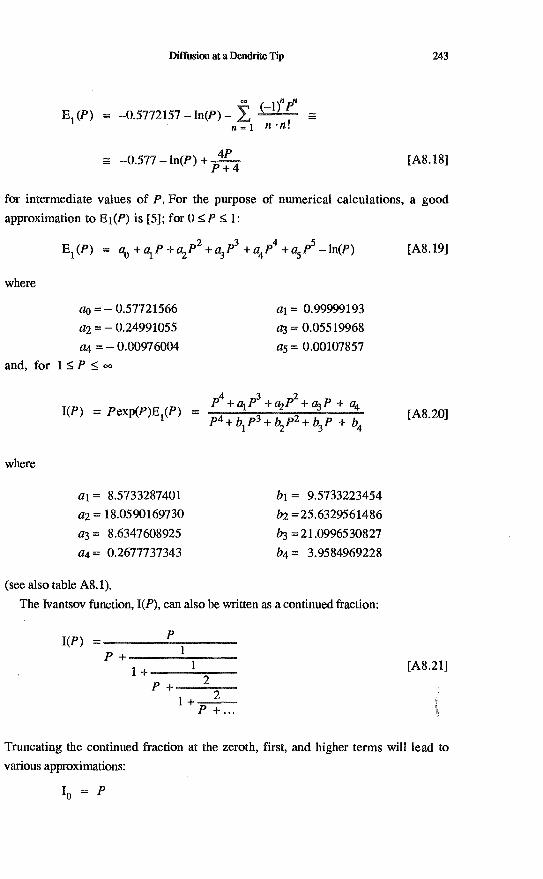
Diffusion at a Dendrite Tip 243
Ε1(Ρ) = —0.5772157 —1η(Ρ) — Σ, (-1)°1°<`
π=1 n·n!
—0.577 —1η(Ρ) + p P 4 [Α8.18]
for intermediate values of P. For the purpose of numerical calculations, a good
approximation to Ει(P) is [5]; for 0 <_Ρ <— 1:
where
Ε1(Ρ) = ac +αΡ +ιι2Ρ2 + α3 Ρ3 +α4 Ρ4 +α5 Ρ5 — hι(Ρ) [Α8.19]
a0 = — 0.57721566
a2 = — 0.24991055
a4 = — 0.00976004
and, for 1<—P <_ oo
αι = 0.99999193
a3= 0.05519968
α5 = 0.00107857
1(Ρ) = Pexp(Ρ)Ε (Ρ) — Ρ4 + α1 Ρ3 +α2 Ρ2 +α3 Ρ + α4
1 Ρ4 + b1 P3 +b2P2+ b3P + b4 [Α8.20]
αι = 8.5733287401 α2 = 18.0590169730 α3 = 8.6347608925 a4 = 0.2677737343
bl = 9.5733223454
b2 =25.6329561486
b3 = 21.0996530827
b4 = 3.9584969228
where
(see also table Α8.1). The Ivantsov function, 1(P), can also be written as a continued fraction:
1(Ρ) _ Ρ
Ρ + 1 1+ 1
Ρ + 2 1+ 2
Ρ + ...
[Α8.21 ]
Truncating the continued fraction at the zeroth, first, and higher terms will lead to
various approximations:
Ιο = Ρ

244 Fundamentals of Solidification
Ι = Ρ 1 Ρ +1
Ι = 2Ρ 2 2Ρ + 1
Ι = Ι(Ρ) = Pexp(Ρ)Ε1(Ρ)
These approximations are shown graphically in figure Α8.4. Substituting the zeroth approximation into equation Α8.14 gives the solution which
was obtained for the case of a hemispherical tip (equation Α8.11). Furthermore, it is
Table A8.1
Ρ Ω = Ι(Ρ) Ρ = -Ω/1η(Ω)# 0.001 0.006338 0.00125
0.002 0.01130 0.00252
0.004 0.01987 0.00507
0.006 0.02743 0.00763
0.008 0.03435 0.0102
0.010 0.04079 0.0127
0.020 0.06845 0.0255
0.040 0.1116 0.0509
0.060 0.1462 0.0761
0.080 0.1757 0.101
0.100 0.2015 0.126
0.200 0.2987 0.247
0.400 0.4191 0.482
0.600 0.4968 0.710
0.800 0.5530 0.933
1.000 0.5963 1.15
2.000 0.7227 2.22
4.000 0.8254 4.30
6.000 0.8716 6.34
8.000 0.8982 8.37
10.000 0.9156 10.4
In this column the Ω-νalυes from column 2 have been used

ιο-4
10'3
Diffusion at a Dendrite Tip 245
interesting to note that the modification of Ζener's analysis, made by Hillert [6] for high
supersaturations, leads to:
~ VR [ C — Co _ Ω D ςο _C* 1— Ω [Α8.22]
which is equivalent to 2P = Ω/(1 — Ω) or Ω = 2P/(2P+1). This is the second
approximation which arises from the continued fraction representation when it is
substituted into equation Α8.14. The paraboloid of revolution, for which the solution is
given by equation Α8.15, represents an isothermal/isoconcentrate dendrite, and closely
approximates the experimentally observed form.
From figure Α8.4, it can be seen that I1 is a much better approximation than is Ip
because the latter cannot be used when P is greater than unity. As the series (equation
Α8.21) converges very slowly, it is usually preferable to use the polynomial
expressions (equations Α8.19 and Α8.20). From equation Α8.22, one sees that another relationship can be obtained for the
inverse Ivantsov solution [7]. This is a good approximation to equation Α8.15 (see table
Α8.1 and figure Α8.4):
ρ = Ω —1η(Ω)
More exact, non-isothermal, solutions have been developed by Trivedi [8].
,. ~
τη / - .
$
,ρ~.•• .
-
: Ω - - Ρ= ιήπ
1(Ρ) τα ~
ί '*~ ~~'
Φ , ~~. ό φ~
- - .
_ *+****i'
i -
~
.,* r -
r~ i .
- i ~ i . ~ ~
. . .. . . ..
' - .
. . ,.
10"α
10-1 Ρ
10
Figure Α8.4
[Α8.23]

246
Fundamentals of Solidification
References
[1] J.C.Fisher, referred to by B.Chalmers in Principles of Solidification, Wiley, New
York, 1966, p. 105.
[2] A.Papapetrou, Zeitschrift fur Kristallographie 92 (1935) 89.
[3] G.P.Ivantsov, Doklady Akademii Nauk SSSR 58 (1947) 567.
[4] G.Horvay, J.W.Cahn, Acta Metallurgica 9 (1961) 695.
[5] M.Abramowitz, I.A.Stegun (Eds.), Handbook of Mathematical Functions,
Dover, New York, 1965.
[6] M.Hillert, Jemkontorets Annaler 141 (1957) 757, and Metallurgical Transactions
6A, (1975) 5.
[7] P.Pelcέ, P.Clavin, Europhysics Letters 3 (1987) 907.
[8] R.Trivedi, Acta Metallurgica 18 (1970) 287, and Metallurgical Transactions 1
(1970) 921.

APPENDIX 9
DENDRITE TIP RADIUS AND SPACING
Growth at the Extremum
The relationships defining solutal (or thermal) diffusion at the hemispherical tip of a
needle-like crystal (appendix 8):
f1 = P [Α9.1]
or a paraboloid of revolution
S2 = 1(Ρ) [Α9.2]
do not specify an unique functional dependence of the tip radius upon the growth
conditions (supersaturation, undercooling). They only relate the product, VR, to the
supersaturation as shown in figure 4.9. Therefore, another equation which links the
variables is required. For many years, this was done by adding a capillarity term to the
diffusion equation and then determining the extremum of the corresponding function.
This approach will be illustrated first by means of the simple solution (equation Α9.1):
S2 = Ρ +
[Α9.3]
where s is the capillarity length (for the solutal case at low Ω-values, s = se = Γ/∆Τok,
and for the thermal case, s = st = Γc/∆hf). In figure Α9.1, relationships such as
equation Α9.3 for various models are presented, in terms of dimensionless variables,
for free thermal dendrite growth and for a constant undercooling, ∆Ι, = 0.05Whf/c [ 1].
These curves indicate that the addition of a capillarity term to equation Α9.1 cuts off the
diffusion solution at some tip radius (see also figure 4.9). The radius at which the cut-
off occurs corresponds to the critical radius of nucleation. This can easily be verified by
noting that this radius is the one which uses up the total supersaturation, indicated by
equation Α9.3, in satisfying the curvature. As a result, V (and therefore P) must be
equal to zero at that point. Therefore:
Ω = 2s R°
(V = 0)

248
Φ
Φ >
10-3
10.4
10-5
10-6
Fundamentals of Solidification
Ι
1
Ω1 =0.05
♦, ~
,_• ».._• ».. ~Spherical ~♦ \ approκ imation
♦ ~
Ν. Ivanesov
Modified .Γ\ Ivan tsov \
1
~/
2-bς5t_
.\ _
\ -
\ - \ Eκ perimentv -
(Glichsrnan) ~
10 10 2
103
104
Figure Α9.1
where the critical radius, R°, for growth is equal to the critical radius, r°, for nucleation.
Substituting ∆Τ for Ω from equation Α8.3 or Α8.6 leads to:
R° = 2s = 2Γ S2 ∆Τ
Examination of equation Α9.3 for the thermal or solutal case reveals that:
∆Τ [Α9.5] Ι 2α c 1 R
∆Τ =2')(
∆Τk ) + R [Α9.6]
C
The extremum (maximum) value of V was thought to define the tip radius (Re, figure
4.9). It is shown in chapter 5 (Fig. 5.7) that the maximum value of V in an isothermal
environment corresponds to a minimum in ∆Τ for constant-velocity growth. Therefore,
minimising ∆Τ in equation Α9.5 or Α9.6 will give the extremum radius and
undercooling. This leads to:
Rt = 2 ( ∆hC)l Ι2µ
1 717 e
∆Τ = 2ΓΓ~~1/2ν 1Ι2
ι \ αι
[Α9.7]
[Α9.8]
r° [Α9.4]

Dendrite Tip Radius and Spacing 249
for thermal dendrites and to
ε ΓD lι l2
Re — 2 ∆Τ k J V ι l2
ο
∆Τ = 2ιΓ∆Τοk,ι/ύι/2
ι l D II
[Α9.9]
[Α9.101
for solutal dendrites when both are growing at the extremum. Equations Α9.8 and Α9.10 reflect the well-known square-root-of-V relationships obtained for free dendrite
growth in a constant supersaturation environment. Others can be found in the review
paper by Glicksman et al. [2].
Instead of using the extremum method, the recent trend has been to use stability
criteria which are analogous to those used in treating the stability of a planar solid/liquid
interface [1, 3-12]. Some simple cases will be treated here which demonstrate the
essential points of the more complete treatments.
Growth at Marginal Stability#
Solution for Dendrite Growth in Undercooled Alloy Melts
The essentials of such an analysis can be rapidly demonstrated in the case of a
thermal dendrite, for example. As the limit of stability of the dendrite tip lies at much
larger rip radii than does the extremum values, the capillarity term in equation Α9.5 can
be neglected and one obtains instead (for a hemispherical needle at low Peclet numbers):
∆Ι = Ρι θ [Α9.11]
where 8, is the unit thermal undercooling (= ∆hf/ι). With Gc = 0 for a pure metal, the
critical tip radius becomes (equation 4.8):
R = [ [Α9.12]
where a* = 1/4π2 and the mean gradient at the tip, G, for the thermal (undercooled)
dendrite can be obtained from G s = 0 (isothermal tip, figure Α8.1) and Gj _ —2Pt®t/R (see exercise 4.6) via the relationship:
# See first footnote in section 4.4.

250 Fundamentals of Solidification
ΚSG, + Κ1Gι [Α9.13]
Κ + ΚI
When κ =
G = Gς η
and, from equation Α9.12:
— ( 2 ,ι/2 ! ~ lι(2V ι/2 Rr ` 11 ι I
r
Substituting equation Α9.15 into equation Α9.11 leads to:
[Α9.14]
[Α9.15]
∆Τ (~1 /2(~Q],` ιl v ι/2 2~ [Α9.161
A comparison of equations Α9.15 and Α9.16 with equations Α9.7 and Α9.8 shows
that both the extremum and the stability arguments lead to qualitatively the same result
(for low Ρeclet numbers) but with differing numerical constants. Thus, the tip radius for
the marginally stable hemispherical dendrite is 4.4 times larger and the undercooling is
2.2 times larger than the corresponding extremum values.
After considering this very simple case, a more complete model will be developed
which is useful for the interpretation of both low and high Ράclet number cases; that is,
dendrite growth under slow and rapid solidification conditions. In the case of alloy growth from the undercooled melt, the coupled transport problem (solute and heat
diffusion) has to be solved. The total undercooling, ∆Τ (= Τ1 — T..), is made up of three
contributions when attachment kinetics are neglected (Fig. Α8.1). These are: ∆Τ,, the
thermal undercooling (T* — T); ∆Τ, the solutal undercooling (Τ — Τ*); and ∆Tr, the
curvature undercooling (Τ1 — Tl ). Two of these undercoolings can be found from the Ivantsov solution for the case of a
paraboloidal tip,
∆Τ = Θ Ι(Pt ) [Α9.17]
where et is the unit thermal undercooling (= ∆hf/c), and:
∆T = mC0 [1— A(Ρ )] [Α9.18]
where

Dendrite Tip Radius and Spacing 251
A(PC ) = Cl*
= [1 - )]-ι [Α9.18α]
(see equation Α8.2). The third contribution to ∆Τ is the curvature undercooling, which is determined by
the relationship:
∆Τ = 2Γ/R [Α9.19]
The sum of the three contributions to ∆Τ gives the total undercooling [8]:
∆Τ = ∆T + ∆T + ∆T [Α9.20]
It has been seen previously that this expression is not, in itself, sufficient to solve the
problem. In order to find an unique solution to equation Α9.20, one can advantageously
use the approach developed by Langer and Muller-Krumbhaar. These authors [1]
proposed a criterion which was based upon extensive numerical calculations. Use of the
criterion gives results which are close to those found experimentally. For instance, see
the points on the curve in figure Α9.1 where the open circle refers to Langer and Miiller-
Krumbhaar's theory, and the closed circle is due to Glicksman et al. [2]. This criterion
supposes that the dendrite tip grows at a constant value of the stability constant,
σ (_ δs/R2: product of the diffusion length, 8, and the capillarity length, s; each made
dimensionless by dividing by the tip radius, R) which is also given by the relationship,
σ = (λ j/2πR)2. Taking the operating value of the stability constant, σ*, to be about
1/4π2, as has been observed experimentally, it follows that:
R = ι11 [Α9.21]
where λί is the lower limiting wavelength for a perturbation which can grow at the
solid/liquid interface. Using this value for the wavelength at a planar interface (equation
3.22) as a zeroth approximation gives [9]:
λ~ = 2π (τl/2 [Α9.22]
Thus at low Ρdclet numbers:
R [
Ι ι/2
σ'(mG — G) (Ρ, P1 « 1) [Ά9.23]
where σ* = 1/4π2. The concentration gradient ahead of an advancing dendrite can be
found from a simple flux balance: VCl (1 — k) = —DG.

252 Fundamentals of Solidification
G _ ~PcC1P ~ R
Substituting for C' from equation Α8.1 and using Ivantsov's solution gives:
G = _ 2ΡρC0Α(Ρ)/R
[Α9.24]
[Α9.25]
In a similar manner, the temperature gradient, G/, in the liquid ahead of a steadily
growing dendrite is found to be:
G _ 2P ∆hf
cR
In contrast to the solute diffusion field, which is evaluated only for the liquid phase,
the temperature field has to be calculated for both phases because of the similarity in
their thermal diffusivities. Therefore, one has to introduce a conductivity-weighted
average temperature gradient. Assuming that κs = Κ/ and that the Ivantsov dendrite is
isothermal, one finds that G at the tip is equal to G112 (equation Α9.14). It is this value
which has to be substituted into equation Α9.23. Substituting equation Α9.23 into
equation Α9.19 then yields an expression for the tip radius:
_ Γ/d` — R
Θ~Ρ [Α9.27]
— 2Ρ mCop Α(Ρ )
where A(PC) = 1/[1 — (1—k)Ι(Ρc)] .
The capillarity undercooling at the tip is therefore:
∆Ι = 2σ*[ Θ~Ρ — 2Ρ mC0 pA(Ρ )] [Α9.28]
The solutal Ράclet number is simply related to the thermal Ράclet number by Pc =
Pt(a/D). Therefore, the only unknown quantity in equations Α9.17 to Α9.20 is the
product, VR (or the Ράclet number). From the definition of Ρ , for example, one can
finally obtain the growth rate:
V = 2ι/ /R [Α9.29]
At high Ρ&clet numbers, this solution has to be generalised by using a modified
stability criterion (appendix 7). Thus one can write, instead of equation Α9.23 [10],
Ι 1/2 R=[ [ σ`(mG* — G* )
[Α9.30]
where σ* is again approximately equal to 1/4π2 and G~ and G* are the effective
[Α9.26]

Dendrite Tip Radius and Spacing 253
concentration and temperature gradients as defined in equation 7.8. Note that, since the temperature gradient in the solid at the tip, Gs, is zero, the product, KSGsξs, is equal to zero in equation Α7.16. Therefore, one can set ξt = 4t (for thermal diffusion in undercooled melts) from now on.
Equation Α9.27 then becomes, in its general form:
R ®
Γld° BtP ~ + 2Ρθξε
[Α9.31]
where θ = ∆Τ Α(ΡC) and ξt = ξι and ξc are defined by equation Α7.23. Substituting equation Α9.31 into the curvature undercooling term (equation Α9.19) and using the other undercooling relationships (equations Α9.17 and Α9.18) in combination with equation Α9.20 gives the general solution for slow or rapid dendrite growth in undercooled alloy melts.
This solution is depicted in figure Α9.2, which shows the variation in the dimensionless growth rate, V = Vst/2a (a), and dimensionless tip radius, R = R/st (b), with dimensionless concentration Co = ColmlO, for succinonitrile-acetone mixtures
at an undercooling of 0.5Κ [8]. The solid line gives the predictions of the present model
and the broken line gives those of more complicated model due to Karnia and Langer
[7]. The points are experimental results from Chopra and Glicksman. For a given (small) ∆Τ, the solution of these equations reveals a maximum in V and a minimum in R with increasing solute content in a given alloy system [8]. For a detailed discussion of
the behaviour of this model for small undercoolings, see reference [8] and for rapid
solidification conditions (large undercoolings), see references [10] and [11].
Constrained (Alloy) Dendrite Growth
During the directional growth of dendrites, the heat generated at the growing
interface does not depend on the tip radius. The latent heat flows into the solid, due to
the imposed temperature gradient. The moving isotherms force the tips to grow at a
given rate into the liquid. Therefore, the resultant growth behaviour (e.g. the tip
undercooling) is determined by the solute flux at the tip. In order to treat this case, one starts again with equation Α9.20, but neglects the thermal contribution to the tip diffusion fields (∆Τ, = 0).
Therefore, for the transport solution one has:
∆Τ = ∆Τ + ∆Τ ε r (G > 0) [Α9.32]
The second equation is deduced from the general stability relationship (equation

254 Fundamentals of Solidificathn
a
0
2- 0 Ο Ο
0
0 .01 .02 .03
Co
b
.04 .05
Figure Α9.2
Α9.30), using the appropriate temperature gradient. Assuming that, at the very tip of
the dendrite, the imposed temperature gradient is the same in both liquid and solid (G =
G1 = Gs) and that the thermal conductivities of the solid and the liquid are equal (K = κ~
= κ8), one obtains for the effective temperature gradient:
G* = (G/2)(ξl + ξs ) [Α9.33]
From equation Α7.23, one sees that ' ι + ξ8 is equal to 2, and the effective gradient is
thus equal to the temperature gradient imposed by the furnace, for example. That is:

Dendrite Tip Radius and Spacing 255
* G =G [Α9.34]
Therefore, the case of columnar dendritic growth is simpler than that of growth from an
undercooled melt. Finally, using the stability expression gives:
Ι ι/2 R = L~(mG ξc—G) ] [Α9.35]
By substituting equations Α9.18, Α9.19, and Α9.35 into equation Α9.32, one finally
obtains the result:
V2A' + VB + G = Ο [Α9.36]
where A' = π2Γ/(Ρ~D2) and B' = Θεξ~/D. This corresponds to equation 7.13.
Since, at high growth rates, the temperature gradient has little effect upon the V-R
relationship of equation Α9.36, it can be neglected. This further simplifies the
relationship, to give:
R2V = DΓ/σ*Θ ξ
[Α9.37]
Note that, at small Pc values, ξc tends towards unity, I(Ρ) tends towards zero, and
8c = ∆Τ0k/[1 —ρΙ(Ρ~)] tends towards ∆Τok. Therefore, setting σ`* = 1/4τε2,
R2V = 4π DΓ/∆Τok, (Ρ « 1) [Α9.38]
which is exactly the same as equation 4.16.
The undercooling can be obtained from equation 7.15 by using the rate-dependent
distribution coefficient of equation 7.3 and the temperature-dependent liquid-state
diffusion coefficient. Figures 7.6 to 7.8 show some results derived by using equation
Α9.36. For more details see reference [12].
Primary Spacing in Constrained Growth
It has been assumed [9] that the shape of a fully developed dendrite, including the
mean volume of its branches, can be approximated by an ellipsoid of revolution
(Fig. 4.14). The radius of an ellipse is given by its semi axes, a and b:
R = b2 a
[Α9.39]
In the case of an hexagonal array, b = λ1/ Ι and a = ∆T'/G, where ∆T' is the non-
equilibrium solidification range. Therefore:

256 Fundamentals of Solidification
3∆Τ'R /2 G 1 [Α9.40]
Substituting equation Α9.38 into equation Α9.40 and replacing, to a first
approximation, ∆T' by ∆Τ0 gives a relationship for the primary trunk spacing:
= 4.3~DΓ∆Το1ιΙαV-ι/aG- ι/τ ι k lI [Α9.41 ]
This relationship is very similar to those derived by Hunt [13] and by Trivedi [14].
The latter extended Hunt's treatment by using the marginally stable tip radius for low
P6clet numbers. Hunt and Trivedi consider the flux balance for a small interdendritic
volume element (Fig. 6.6), where the cell/dendrite axis is the z-axis, and r is the radial
distance. Summing the radial solute concentration change,
f (αες /αt) = (af /αt)C/ (1 - k)
and longitudinal solute concentration change,
(act /at) = a[D(8c /ακ)va~
gives:
J, (αCς /λt) = (8f5 /at)C1 (1 - k) + d [Dj (9c /ax)]/ax [Α9.42]
Setting G = m(aC1/αχ), and assuming the existence of a constant interdendritic
concentration gradient (9C1/ 2- 0) leads, since af)/αχ = - (1/V)(afς/λt) under
steady-state conditions, to:
f dC, = [C~ (k-1) - (DG/mV)]9f [Α9.43]
Integrang from f~ = 1 to f~ and from Cι = C to Ci gives:
f (k-1) = [C1 (k- 1) - (1)0/mV)]/[C, (k-1) - (DG/mV)] [Α9.44]
For a cylindrical geometry, one hash = [1 - r2/(λι/2)2]. Substituting this expression
for fi and fitting a spherical tip to the 'Scheil-cell' finally leads to [ 13]:
R= - Gλ?
[Α9.45] 5.66 [mCς (1- k ) + (DG/mV )]
Following Tńvedi [14], and using the results derived for the dendrite itself, one can
substitute for the tip radius and concentration (equations Α9.37 and Α9.18a,
respectively). Using the low Ράclet number approximations: Α(Ρ) -- 1 and s -*1,

Dendrite Tip Radius and Spacing 257
gives:
λ1 = 6(∆ΤΟ kDΓ)ιIaV 114G 1'2[1 - (DGIV®Τοk]tlτ [Α9.46]
Α comparison of equations Α9.46 and Α9.41 reveals a similar behaviour at the small
G/V ratios which are typical of dendrite growth. If DG/V∆Τ0k tends towards unity,
cells will be the preferred morphology and the spacing increases with increasing V.
In summary, it should be pointed out that, with regard to λ1, none of these models
represents well the real behaviour, as described by Esaka and others [15]. They are
useful only for making qualitative estimates of λ1, rather than for making precise
predictions.
Secondary Spacing in Constrained or Unconstrained Growth
In order to simplify the model, it is assumed that only two dendrite arms of different
diameters need to be considered. In reality, a distribution of arms of various thickness
will exist.
Following Kattamis and Flemings [16] and Fearer and Wunderlin [17], the situation
illustrated in figure Α9.3 will be analysed in a very approximate manner. Two arms of
radius, R and r, are placed in a locally isothermal melt. Since, at the interface between
the solid and the liquid, local equilibrium will be established very rapidly, the
concentration along the surface of the cylindrical arms will differ; the thinner arms will
be in liquid of lower solute concentration. That is:
= Tf + mCR —
Τ = Τ!
+ mCP— Γ
For an isothermal system, one therefore obtains:
m(CR — CÍ) = r( - 1) [Α9.47]
Solute will diffuse along the concentration gradient from thick to thin arms while the
solvent will diffuse from the thin to the thick arms. The thin arms therefore tend to
dissolve while the thicker arms tend to thicken.
For simplicity, it is assumed that the concentration gradient between two arms is
constant and that the diffusion is unidirectional. Now, if R is assumed to be much
greater than r, dR/dt can be neglected with respect to dr/dt, and the two fluxes existing
between the arms are:

τ τ, Τ.
258 Fundamentals of Solidification
λΖ
Figure Α9.3
J - D (CR —c,) d
J = —Cί(1—k4
Combining equations Α9.47 to Α9.49:
[Α9.48]
[Α9.49]
ΓD (1 1l mq (1 _ k)d l r R
For small compositional differences in the liquid between the arms, C'1 is approximately equal to C1; the interdendritic concentration due to segregation. It is
further assumed that d is approximately equal to the arm spacing, leading to:
dr ΓD ‚-1 1 ~ dt mCl (1 —k)λz r R [Α9.51]
0
where λ2 is the arm spacing before ripening. All of the parameters, except Cl on the
right-hand side of equation Α9.51, are assumed to be constant. Furthermore, it is 0
assumed that R/~2 and rp/R are constant and that the interdendritic liquid concentration
is a linear function of time; starting with the alloy concentration, Co, and ending (due to
segregation) at the composition, Cl :
C, = Co + (Cl — ς)~ [Α9.52] f
dr dt [Α9.50]

Dendrite Tip Radius and Spacing 259
where t is the time elapsed since the start of solidification, and tf is the local
solidification time. If Cl = Ce, tf is approximately equal to (T1— Te)/t .
Rearranging equation Α9.51 and integrating from t = 0 to t= tf and from r = ro to r = 0 gives:
where:
λzR2 [R + In(1 — R—° )] = ΜΊ [Α9.53]
Μ = — iDln(Ci /Co )
[Α9.54] ιιτ(1 —k)(C1 —Co )
Feurer and Wunderlin [17] then assume that R/λ2 = 0.5 and that ro/R - 0.5, which 0
gives Mtf = 0.1 (λ 2)3. Furthermore, they suppose that, when the arms have melted,
λ2 = 2λz and therefore:
λ2 = 5.5(ΜtJ.)113 [Α9.55]
Due to the extreme simplification of the ripening phenomena described, the constant
factor of 5.5 in equation Α9.55 should not be accorded too much significance. This
applies to both its value and its constancy. Nevertheless, the coarsening parameter, M,
has been shown to be of some use in estimating Ά2 values in Al alloys [17]. However,
it should be kept in mind that the coarsening described here relates to the secondary
branch spacing next to the primary trunk. This is so because, when one measures λ2 at
points far from the trunk, one misses the finer dissolving branches.
Because the real situation is here again very complicated, numerical studies of the
behaviour of distributions of aims or particles as a function of time can be very useful in
obtaining a better understanding of coarsening in general [18]. As a result, improved
modelling of microstructural changes becomes possible [19].
References
[1] J.S.Langer, H.Miiller-Krumbhaar, Journal of Crystal Growth 42 (1977) 11.
[2] M.E.Glicksman, R.J.Schaefer, J.D.Ayers, Metallurgical Transactions 7Α (1976)
1747.
[3] W.Oldfield, Materials Science and Engineering 11 (1973) 211.
[4] J.S.Langer, Reviews of Modem Physics 52 (1980) 1.

266 Fundamernals of Solidification
[5] J.S.Langer, H.Miiller-Krumbhaaτ, Acta Metallurgica 26 (1978) 1681, 1689 and
1697.
[6] J.S.Langer, Physico-Chemical Hydrodynamics 1 (1980) 41.
[7] A.Karma, J.S.Langer, Physical Review Ά30 (1984) 3147.
[8] J.Lipton, M.E.Glicksman, W.Kurz, Metallurgical Transactions 18Α (1987) 341.
[9] W.Kurz, D.J.Fisher, Acta Metallurgica 29(1981)11.
[10] J.Lipton, W.Kurz, R.Tnvedi, Acta Metallurgica 35 (1987) 957.
[11] R.Trivedi, J.Lipton, W.Kurz, Acta Metallurgica 35 (1987) 965.
[12] W.Kurz, B.Giovanola, R.Trivedi, Acta Metallurgica 34 (1986) 823, and Journal
of Crystal Growth 91 (1988) 123.
[13] J.D.Hunt, Solidification and Casting of Metals, The Metals Society, Book 192,
London, 1979, p. 3.
[14] R.Tńvedi, Metallurgical Transactions 15Α (1984) 977.
[15] H.Esaka, W.Kurz, R.Tńvedi, in Solidification Processing 1987, The Institute of
Metals, London, 1988, p. 198.
[16] T.Z.Kattamis, M.C.Flemings, Transactions of the Metallurgical Society of AIMS
233 (1965) 992.
[17] U.Feurer, R.Wunderlin, Fachbericht DGM, 1977 (see detailed reference in
chapter 4).
[18] P.W.Voorhees, M.E.Glicksman, Metallurgical Transactions 15A (1984) 1081.
[19] W.Kurz, M.Rappaz, in Solidification des Alliages, Ecole d'et6, Carry-le-Rouet,
1985, Les ditions de Physique, France, 1988, p. 191.

APPENDIX 10
EUTECTIC GΊ OWΤΗ
Low Ρeclet Number Solution
This appendix follows, in its first part, the treatment of Jackson and Hunt [1], but is
a simplified version of the latter paper. Figure 5.2 shows the corresponding phase
diagram and interface geometry. Using symmetry arguments (appendix 2), the analysis
of a solidifying lamellar eutectic interface can be reduced firstly to the consideration of a
pair of lamellae. No net mass transport can occur between this pair and another pair
under steady-state conditions because this would cause changes in the morphology and
violate the assumption of steady-state behaviour. Thus, the concentration gradient in the
y-direction is zero at the mid-point of each lamella (Fig. A10.1). Secondly, attention
can be further restricted to half of each lamella because, again, there can be no net
transport of solute in or out of this symmetry element.
The differential equation describing the solute distribution in the melt ahead of a
steadily advancing interface is:
d 2C + d2C + V dC = 0 [Α2.6] áy 2 r%z 2 D dz
and it has been shown (appendix 2) that the general solution satisfying this equation
consists of products of circular and exponential functions. It is logical to associate the
exponential function with the z-variation of the solution, since it is known that the
boundary layer has this form for a single-phase interface. It is equally logical to
associate the circular functions with the alternating pattern of eutectic phases. Thus,
merely by inspection, the distribution of component B can be deduced to be of the form:
C = ς ±Α exp(— D)+ Bexp(—bz)cos(gy) [Α10.1]
This approximate solution# can be seen to be made up of an exponential term which
reflects the planarity of the interface as a whole, and another term which reflects the
The exact solute profile must be described by a sum of circular functions rather than by just one term. However, this choice simplifies the treatment without losing sight of the important physical phenomena.

262 Fundamentals of Solidification
λf/α λc1-f>/α
λ/2
Figure A1O.1
alternating pattern of the two phases. The cosine, rather than sine, function is chosen
because the expression describing the gradient of the interface concentration in the y-
direction must be able to take zero values at the origin of the region considered and at
λ/2 (Fig. A10.1). Another way of regarding the choice of the function in equation
A10.1 is to imagine that it reflects the interface solute distributions depicted in figure
5.3. Thus, equation A10.1 without the third term on the right-hand side, and with a
suitable choice of value for A, could describe the solute distribution ahead of either of
the single phases (Fig. 5.3a). The re-introduction of the third term can then be looked
upon as being the expected solution when the originally single phase interface is
'perturbed' by the addition of the second phase (Fig. 5.3b).
It is now necessary to determine the constants, A, B, b, and g. The value of g can be
immediately determined because, again due to symmetry considerations, the derivative
of the solution with respect toy, 9C/9y, must be equal to zero when y = λ/2. Thus:
C = Ce +Α exp(— - ) + Bexρ(—bz)cos()
The derivation of b has already been discussed (equation Α2.10). It is equal to:
b = + [(Υ)
2 +( 2 l2 η 1/2
[Α 10.2]
[A 10.3]
This relatively complicated expression can be simplified on the basis of experimental
observation. Firstly, it is noted that the term, V/2D, is the inverse of the equivalent
solute boundary layer of a planar interface. At low growth rates its value will be

Eutectic Growth 263
relatively small, whereas 2n/λ is the wave number of the eutectic and will be large, due
to the small values of 'l which are usually encountered. Therefore:
4π2 » V2 λ2 4D2
and equation Α10.3 can be simplified to:
b _ 2π (P « 1)
by neglecting terms in V/2D (Ρ = Vλ/2D). Thus, equation Α10.2 can now be written:
C = Ce + Α exp(— . ) + Β exp(— λZ )cos(f.)
[Α 10.4]
The values of the constants, A, B, can be found by forcing the above solution to
satisfy the flux condition at the interface. The fluxes can be deduced from the phase
diagram. The general flux boundary condition is:
V(k-1)C* = D(~Z)Z _ o [Α10.5]
but, because the variation of the interface concentration with respect to Ce is relatively
small in most cases except rapid solidification, it can be supposed that C* = Ce.
Thus, the flux conditions for the two eutectic phases can be written in terms of the
weight fraction of element B as:
α-phase: V(k-1) e = D(. ) =
β-phase: —V(kβ -1)(1—C) = DaZ~Z=o
[Α 10.6]
[Α10.7]
The negative sign in the case of the /3-phase appears because the interface gradient of CB
in the growth direction is expected to be positive. The concentration gradient at the
solid/liquid interface can be found from equation Α 10.4:
(-,9C
-) - ο = —DA — λ Bcos(~λ.)
[Α10.8]
The α-phase extends from the origin to the point, fλ/2, where f is the volume
fraction of the α-phase (as has been defined in reference [1]).
Using the method of 'weighted residuals' (appendix 2), the values of A and B (the
'weights') can be found by satisfying the flux boundary conditions (equations Α10.6 and Α 10.7) in an average fashion over the a and β interfaces, i.e.:

C φ C'
∆Τg /~j\ \ ∆Τ~
∆CρΊ ΛC α
C'
264 Fundamentals of Solidificadon
a a 2 2
fV(k~ -1) CdΥ = JD(.) = 0dy
ο ο
λ λ
ι
2 f2
νίιίβ - 1) (1- C )dy = iD ( ατ )z οdΥ a a 2 2
[Α10.9]
[Α 10.10]
Inserting the value of (6C/rΖ),Ο from equation Α10.8, and carrying out the integrations
yields the simultaneous algebraic equations:
fVλA + 2Dsin(πf)Β = (1 —k~ ) CfVλ
(1 — f )Vλλ — 2sin(πf )Β = (kβ — 1)(1 — C )(1 — f )Vλ
and the values of Α and Β are easily found to be:
Α = fC'—Cs
Β _ f(1—f)VλC' 2Dsin(πf )
[Α10.11]
[Α 10.12]
[Α10.13]
[Α 10.14]
Note that Α will be very small in general, and will be equal to zero if the phases have
the same density. Here, C' is the difference in composition between the ends of the
eutectic tie-line and Cβ is the difference in composition between the eutectic and the
maximum solid solubility in the β-phase (Fig. Α10.2).
Figure Α10.2

Euteclic Growth 265
Thus, a solution has been obtained which satisfies most of the boundary conditions.
The final condition to be satified is the coupling condition, which relates the local
melting point to the imposed temperature distribution. This has already been depicted in
a qualitative fashion in figure 5.5. If account were to be taken of the detailed shape of
the eutectic interface, the problem would rapidly become intractable because of the need
to satisfy the coupling condition at each point#. Instead, the eutectic interface is assumed
to be perfectly planar, in order to make a solution possible, and the quantities involved
are treated in an average fashion. The satisfaction of the coupling condition can then be
achieved in three steps. These involve calculating the average solute undercooling and
the average curvature undercooling for each phase, and then equating the two total
undercoolings.
The average concentration differences of the liquid, ∆C = C — Ce, at the α- and β-
phase interfaces, relative to the eutectic composition will first be found. From equation
Α10.4, they can be shown to be, for z = 0:
.fλ 2
= ..%f[A +Bcos(..Ξ2)]dy α
λ
β = (1 f )λ
Ι[Α +Βcοs(λ
)]dy
giving:
θC = Α + Β
α πf
θC = Α Β sίη(πf ) ~e(1 -f)
[Α10.15]
[Α10.16]
Since Α is usually negligible and B is positive, it can be seen that the average
concentration difference in component B at the ct-phase interface is positive, while that
at the β-phase is negative. The mean solute undercoolings, with respect to the eutectic
temperature (Fig. 5.5), can be found by multiplying the above concentration
differences by the absolute liquidus slopes, Ιm'd and mill. The solute undercoolings are
# Series et al. [2] have solved this mathematically difficult problem by using a hybrid method in which an electrical analogue was used to provide data for further calculations.

z" ή — 2 3/2 (1+τ') [Α 10.19]
266 Fundamentals of Solidification
therefore:
λf/2 λ(1-f)/2
Figure Α10.3
α = 1m Ι ΓΑ + B sιηπ(nf)J
f
β [Α Β sin(nf ) l θΤ = — Ιmβ Ι n(1—[)
[Α10.17]
[Α10.18]
since both of them are positive.
The second source of undercooling to be considered is the average undercooling due
to the curvature of the interface. Firstly, note that the average curvature of a line
between two points which are a distance, L, apart can be found by integrating the
general expression for the curvature (appendix 3),
between the two points. Thus:
L
o (1 + Ζ Q)3/2
Making the successive substitutions, Z = i and tan() = Z (Fig. Α10.3) leads to:
= L [sin(θ)]ó
Again using the above identities leads to:
=
sin[arctan(z')]~ [Α 10.20]
The form of the eutectic interface is assumed to be as shown in figure Α10.3. Thus,
the average curvature of the β-phase can be found by substituting the slopes at y = fλ/2
Κ =

f λ ∆Τα = 2Γα sίη(θα )
~ [Α 10.21 ]
Eutectic Growth 267
and λ/2 into equation Α10.20:
Κ — 2sin(%)
α fλ
Κ _ 2sin(θβ )
β (1-f)λ
The curvature has been defined to be positive if the solid projects into the melt.
Mathematically spealdng, it is negative. The curvature is defined differently here so as
to give a positive undercooling (for a solid projection) when combined with the
(positive) Gibbs-Thomson coefficient. Therefore, using the associated Gibbs-Thomson
coefficients, the curvature undercoolings become:
∆Τβ — 2Γβ sin(θβ) (1—f)λ
[Α 10.22]
Combining equations Α10.17 or Α10.18 with equations Α10.21 or Α10.22 gives the
total undercooling of the two phases:
sin(πf ) 2Γα sin(Θα) ∆ά = Ι á rn Ι[Α+Β πf ] + f λ
θΤ = -Im Ι [Α Β sin(πf ) j + 2Τ' sin(Θβ) ~ β π(1 -f) (1 —f)λ
[Α 10.23]
[Α 10.24]
Multiplying equation Α10.23 by Imjj and equation Α10.24 by Im α1 , and adding gives:
Ιm Ι∆ά +Ι άΙ∆~
= Ι αΙΙmβΙ B πιη1π f) + β f( f)
2ΙmβΙΓ sin(Θα )
fλ
2Ι άΙΓ sin(Ο) [Α 10.24a]
(1—f)λ
However, the coupling condition (appendix 2) requires that the α- and β-interfaces
should lie on the same isotherm. Due to the very small distances between the phases

268 Fundamentals of Solidification
(typically of the order of a few microns) and their high thermal conductivities, no
substantial temperature difference can exist between the α and β phases. Therefore,
∆T a = ∆Τβ = ∆Τ (Fig. 5.5):
∆T = 1 ml Ιmsl B sin(πf) + 2 Ι'Ι α sin(Q) +
1m Ι+Ιmβ Ι πf(1—f) fλ(Ιmm l+Imβ l)
21ma1 Γβ sin(Θβ) +
(1 —f)λ(Ima1+1mβ1)
Substituting for B from equation A10.14 gives:
ΙmallmΒΙ νλS.
+ Im l + Imβl 2πD a
2(1 f)Ι n Ι άsin(θα )+2f ΙmαΙΙ sin(θΒ )
f(1— f)λ(I αΙ+ Imβ1)
This can be written (see also equation 5.8):
∆Τ = K νλ+ λ C
where the physical constants of the alloy are:
I αl Ιm1 Ι ς Κ l ál + lm~1 2πD
and
2(1 f)Imbl ásin(Θα )+2fIma lΓ sin(θβ ) Κ = r 1( 1 —f )(l άl + Ιmβι)
∆Τ
[Α10.25]
[Α 10.26]
[Α 10.27]
[Α10.28]
[Α 10.29]
Assuming that the λ-value chosen by the eutectic is the one which makes ∆Τ a
minimum, i.e.:
d(∆Τ) = Κ ν — Kr = 0 dλ ` λ2
it is found that:
2 K, 4nD f ΙmαΙΓ sin()+ (1 f)Irr ι'1 ά sίη(θα ) λ ν = χ
= f(1 f) i άι ιmβι ς' [Α10.30]
~

Eutectic Growth 269
Finally, it is interesting to compare the approximate solution above with the more
exact derivation performed by Jackson and Hunt [1]. Writing their expression for λ2V
in terms of the nomenclature used in this book gives:
λ2ν = ZD f ΙrηαΙΓ sin(®β ) + (1 f )ΙmβΙ ά sin(®α ) Ρ ' Ima l ΙmβΙ C'
[A10.31]
where Π = Σ(1/n3π3)sin2(nι '). Equations Α10.30 and Α10.31 differ only with respect to the first multiplying term
on the right-hand side. The relationship is seen even more clearly if one writes their
equivalent expressions for Κ, and Kr for the J.H. model:
C f(1 -f)D
Κ = 2m Γ sin(®α ) + Γ sin()1
f lmal (1 —f) Ιmβ Ι
with in= Ιm α l l mβ l /( Ιma l+ Ιmβ l ). If the complicated expression, P' (equation Α10.31), is compared with the equivalent
expression, f(1 f)/2ππ, the agreement is found to be quite reasonable (table A10.1) in
spite of the comparative simplicity of the above derivation. As one would expect from
the symmetrical form of the approximate solution used, the accuracy is greatest for f-
values of about 0.5.
Table 410.1 Comparison of Terms Appearing in the Jackson-Hunt (JH) and Present Analyses#
f 100
P = Σ(1/n3π3)sin2(n ιΙ) (JH) 1
(f Í2)/2π Error(%)
0.1 0.00626 0.01432 129
0.2 0.01633 0.02546 56
0.3 0.02553 0.03342 31
0.4 0.03174 0.03820 20
0.5 0.03392 0.03820 17
(the results for higher f-values are symmetrical about f = 0.5)
Another useful approximation is Ρ. = 0.335[f(1 _ j)]165 A similar expression can also be derived for rod eutectics [5].

270
f
Table Α10.2
Fl
Fundamentals of Solidification
Values of the P Function (J.-H. Model)
f Fl
f F'
0.00 0.00000 0.17 0.01327 0.34 0.02845
0.01 0.00014 0.18 0.01429 0.35 0.02909
0.02 0.00046 0.19 0.01532 0.36 0.02970
0.03 0.00091 0.20 0.01633 0.37 0.03027
0.04 0.00147 0.21 0.01734 0.38 0.03080
0.05 0.00212 0.22 0.01833 0.39 0.03129
0.06 0.00284 0.23 0.01930 0.40 0.03174
0.07 0.00362 0.24 0.02026 0.41 0.03215
0.08 0.00446 0.25 0.02120 0.42 0.03252
0.09 0.00534 0.26 0.02212 0.43 0.03285
0.10 0.00626 0.27 0.02301 0.44 0.03313
0.11 0.00721 0.28 0.02388 0.45 0.03337
0.12 0.00819 0.29 0.02472 0.46 0.03357
0.13 0.00918 0.30 0.02553 0.47 0.03372
0.14 0.01019 0.31 0.02631 0.48 0.03383
0.15 0.01121 0.32 0.02705 0.49 0.03390
0.16 0.01224 0.33 0.02777 0.50 0.03392
For the purposes of making more exact calculations using equation Α10.31, an
expanded table [3] of F' values is given in table Α10.2.
Eutectic Growth at High Rates
The main difference between the analysis of eutectic growth at high and low rates is
that, in the former case, one cannot make some of the simplifying assumptions which
were made earlier in this appendix.
The first difference is that one cannot assume that 47c2/λ2»V2/4D2, because V is
now also very large. The second difference is that one can no longer assume that the
interface composition in the liquid is close to the original eutectic one. Therefore, the
interface gradients are now functions of the interface concentrations, and the exact
solution of the problem becomes much more difficult. In fact, a solution has been
developed [4] by making the assumption that kα = kβ. In the approximate derivation which follows, it is not necessary to make this
simplification, but it will be retained anyway in order to facilitate comparison with the
more exact result [4].
Starting with equation Α10.2, one again finds an expression for the concentration

Eutectic Growth 271
gradient in the liquid at the interface:
aC/az = — (VID)A — bBcos(2πy/λ) [Α10.32]
Note that one cannot here assume that b = 2π/λ . One must later insert this
expression for the gradient into equation Α10.5 giving, since one has to assume that the
liquid composition at the interface, C,, is not equal to Ce:
V(k — 1)C = D(aC/?z) [Α10.33]
V (k — 1) (1 — C ) = D (aC/ατ )~ = π [Α 10.34]
Recall that it is assumed that kα = kβ = k.
The composition at the interface is:
i
= C + Α + Bcos(2πy/λ) [Α10.35]
It is now necessary to set up equations which are equivalent to equations Λ10.9 and
A1O.10. This gives, upon substituting from equations Α10.32 and Α10.35:
fλ 2
V(1 —k) f (C +Α + Bcosψ)dy = ο
R i
= D f(~Α + bBcos 2λ )dy ο
[Α 10.36]
λ
V(1—k) f (1—C— Α —Bcos 2λ )dy = fλ τ
λ 2
= D f(- DA—bBcos~)dy fλ 2
[Α ΣΌ.37]
This leads to two simultaneous algebraic equations which are equivalent to equations
A10.11 and Α10.12:

272 Fundamentals of Solidification
Ρ(1—k)[( C+Α)f+ πsίηπf] = PAf + bB2 sinnf [Α10.38]
Ρ(1—k)[(C +Α —1)(1—f )— π sinnf ] = ΡΑ(1 f)—bB 2nsίηπf [Α10.39]
where P is the Pdclet number (= Vλ/2D). Adding the two equations and simplifying
gives:
Α = [(1 —k)/k][fC — (1—f)(1—C )] [Α10.40]
This is the equivalent equation to equation A 10.13, and Α is identical to Βo in equation
15a of reference 4.
Multiplying equation A10.38 by (1 —f), multiplying equation A10.39 by f, and
subtracting one from the other leads, after substituting for b from equation A10.3, to:
Β ® Ρ (1 — k)(fI — )(2πlP) sin(πf )((1 + (2π/Ρ)2)1~ — 1 + 2k)
[Α 10.41 ]
The calculations can now be carried forward in exactly the same way as for the low-
velocity case, but using the new values of Α and B. For instance, the average
concentration difference ahead of the a phase is now:
∆ ά = 1kk [fC- (1 f )ί1---c )] +
(f—f2)1 k) + λV Γ 2π Ρ 1
7Π L (1+( p )2)ι/2
— 1 + 2k J [Α 10.42]
The expression in the large bracket on the RHS of equation A10.42 is equivalent to
the exact function, P(f,p,k), to be found in reference [4]. It has been written in the
present form so as to reveal the similarity. Note that the factor, (f — f2)/2π, is the
simple solution in table A10.1.
The overall effect of high growth rates can be seen by replacing B, in equation
Α10.24a, by the expression in equation Α10.41. This gives:

where
Κ — Ima llmβl 1— k (2π/Ρ)
Im I + ΙmβΙ 2πD [1+(2π/Ρ)2] ι12-1+2k α [Α 10.44]
Eutectic Gmwtb 273
That is:
1m 11m1 2~ (1—k) 2π/Ρ
∆Τ — α Β + Ι άΙ + Ιmβ1 [ 1+(2π/Ρ)2] ιl2 — 2k + 1
+ 2(1—f )ΙmβΙ ά sin(Oa ) + 2f ΙmαΙΓβ sin()
f (1 f)λ(Im«Ι+Ιmβ1)
∆Τ = Κ Vλ + Κ/λ
[Α 10.43]
Compare this with equation Α10.28 and note that (1 — k) corresponds to C. Also, Kr is given by equation Α10.29. Hence, after optimisation:
_ 4πD [1 + (2π/Ρ)2] ι~ — 1 + 2k f(1 f) (2πlΡ)
, f ΙmαΙΓβ sin() + (1 — f )ΙmβΙ ά sin(Oa ) Ι άΙ ΙmβΙ(1 — k)
[Α 10.45]
It is of interest is to see hbw this high growth rate (high P) solution differs from the low Ρόclet number solution. This is quickly done by separating out the P-dependent
terms. Thus:
λ2V = D® (Ρ2± 4π2)112 — Ρ + 2/CΡ 2π(1 — k)
[Α 10.46]
where Θ is a constant which groups together all of the fixed parameters which appear in
equation Α10.45. Note firstly that the RHS of equation A10.46 tends to
λ2V = D®/(1— k)
when Ρ tends to zero; which corresponds to equation A10.30 and indicates that λ2V is
independent of the growth rate. By differentiating equation Α10.46 with respect to P
and equating the result to zero, one finds that the λ2V versus P curve has a minimum
when:
λ2V

274 Fundamentals of Solidification
P _ π(1 —2k) [k(1 —k)] 112
In fact, there is no minimum if k is greater than 0.5 (Fig. 7.12).
As P tends to infinity, equation A10.46 tends to the value:
[Α 10.47]
λ2V = Dθ π(~k)
Thus, λ2V is no longer constant, as in the low-P Jackson-Hunt solution, but
increases with P at a rate which depends upon k. In equation A 10.47, note that the
minimum moves rapidly towards infinity as k tends to zero. As a result, the curve can
be expected to decrease monotonically towards zero.
As might be expected, the predictions of the simple expression are very inaccurate
for small values off (as in table A10.1). They also diverge badly from the exact values
when k is large. This is also to be expected in view of the difficulties of convergence
which are encountered when using numerical methods [4]. However, even when the
absolute values predicted by the simple equation are inaccurate, the relative values over
a range of k- or f-values are generally adequate. Thus, the simple expression can be
used with confidence in exploring the qualitative behaviour of the solutions, and aids
physical understanding.
References
[1] K.A.Jackson, J.D.Hunt, Transactions of the Metallurgical Society of the ACME
236 (1966) 1129.
[2] R.W.Series, J.D.Hunt, K.A.Jackson, Journal of Crystal Growth 40 (1977) 221.
[3] J.N.Clark, J.T.Edwards, R.Elliott, Metallurgical Transactions 6A (1975) 232.
[4] R.Trivedi, P.Magnin, W.Kurz, Acta Metallurgica 35 (1987) 971.
[5] R.Trivedi, W.Kurz, in Solidification Processing of Eutectic Alloys (Eds.
D.M.Stefanescu, G.J.Abbaschian, R.J.Bayuzick), The Metallurgical Society,
1988, p. 3.

APPENDIX 11
TRANSIENTS IN SOLUTE DIFFUSION
Initial Transient
As shown previously (chapter 3), the build-up of solute ahead of a planar solid/liquid
interface takes some time - the time required for the saturation of the diffusion boundary
layer. It is assumed, to a first approximation, that diffusion is rapid enough to ensure,
during this transient, the existence of a quasi-steady-state solute distribution. In this
case, the concentration decreases exponentially from the interface into the liquid, and the
equivalent boundary layer is always of the same thickness (appendix 2):
δ = 2D c µ
Assuming that the growth rate, V, increases instantaneously to a constant value at the
start of solidification the flux at an interface of unit area, due to the differing solubilities
of the solute in the two phases, will be:
Jt = VC,#(1—k)
[Α11.1]
Initially, this flux is greater than the flux created by the concentration gradient in the
liquid:
J2 = —DG [Α11.2]
The difference between the two fluxes will be used to 'fill' the diffusion boundary
layer, of thickness δ~, to a mean concentration, Cr
Jt —Jz = t δ [Α11.3]
Recalling that a quasi steady-state profile is assumed to exist, the concentration
gradient at the solid/liquid interface is given directly by the first derivative (at z = 0) of
equation 3.2, with ∆C0 in this transient state being replaced by ∆C = (C j — C0)
(Fig. A11.1):

276 Fundamentals of Solidification
G = (Co — ζ .
[Α11.4]
Therefore, for unit area:
J2 = —00 )V
and from equation A11.3
2D d~
= kCl*) V dt
[Α11.5]
Noting that, for the triangular equivalent boundary layer (fig. A11.1b), the variation
in the mean concentration is related to the variation in interface concentration, e.g.:
a
b
dz '
Figure A11.1

•—grad C • 0
υ
Transients in Solute Diffusion 277
dς = dG 2
with V = dz%dt:
* Cod ς* = D dz
Integrating:
*
JdG —
D J c
Co —kς* D o
ο
gives:
~~Co (1—k) ] τlk — Vz'
Ζ —~
Π =.
Figure Α11.2
[A11.6]

278 FυndamenιaΙe of Soliditicatkrn
or
= ~ [1 — (1—k)exp( kD)1 [Α11.7]
Figure 6.2 illustrates the behaviour of this expression. It is a good approximation to
the exact solution derived by Smith et al. [1].
Final Transient
While the initial transient is required to build up a boundary layer, the fmal transient
is the result of the 'collision' of the boundary layer with the end of the specimen
(Fig. A11.2). This problem has been solved by Smith et al. [1] in the following way
for the case where the system has reached a steady state. The origin of the z-axis is
placed at the end of the specimen and the diffusion equation becomes, in terms of the
new x-coordinate (which does not move with the solid/liquid interface);
d2Ci _ l dCl
dx2 D ut
The boundary conditions apply for all values oft. At x =0 (the end of the specimen)
the diffusion flux must be equal to zero and:
dCl _ 0
dx
and at the solid/liquid interface, x = x*:
dc, _ ν dx 5 tP
[Al 1.9]
[Α11.10]
where x* is the length of the liquid zone.
In order to meet the first boundary condition, an imaginary source placed in a
symmetrical position with respect to the real solid/liquid interface is introduced. This is
equivalent to a barrier to mass flux being placed at the end of the specimen
(Fig. A11.2). The steady-state distributions at the two interfaces in an infinite specimen
are:
Ct = Co(l+~ )eχρ[ µ(xDχ)
~
[Α11.11]
where z = x* ± x. In order to cope with the second boundary condition (equation
A11.10) when the sources are close enough to interact, further sources (interfaces) are
introduced at distances, nx*, where n is an integer (Fig. A11.3). These sources travel
[Α11.8]

Transients in Solute Diffusion 279
J
Figure Α11.3
at speeds which are n times the speed of the real interface. This superposition permits
the calculation of the necessary coefficients by constraining the interface to obey the flux
balance (equation A11.10):
= 1+ xi 1exp[—nD(nx* — χ)]+ exp[—nD(ηχ* +χ)] [Α11.12] ο η =1
This procedure is given in more detail in the original reference [1] and leads to:
C (x) = 1+3 1—k exp~— 2Vxl + 5(1—k)(2—k) l+k D J (1+k)(2+k) D
+ (2n + 1) (1—k)(2—k)...(n—k) exp[_ n(n+l)Vxi [Α11.13]
(1+k)(2+k)...(n+k) D
The above equation describes the final transient in the solid for the case where a
steady-state solute pile-up has been established at the solid/liquid interface.
References
[1] V.G.Smith, W.A.Tiller, J.W.Rutter, Canadian Journal of Physics 33 (1955)
723.

APPENDIX 12
MASS BALANCE EQUATIONS
The different solubilities of a solute in the liquid and solid phases, together with
differences in mobility, lead to the spatial concentration variations known as
segregation. Provided that the mass transport in the liquid is infinitely rapid (no
concentration gradient in the liquid), the corresponding relationships can easily be
derived from a mass balance (where C is expressed as a percentage):
fC +fCl = 100
[Α12.1] ά(6ς) + c1~Cl ) = 0
These equations state that all of the solute which cannot be incorporated into the solid
must enter the liquid. No account is taken here of all of the other possible phenomena
which might occur in a practical situation. For instance, solute vaporization or crucible
reaction.
Lever Rule
The simplest case to which a mass balance can be applied is that of equilibrium
solidification (no concentration gradient in the solid or liquid). This can be expressed by
the relations:
D » D » LV [Α12.2]
Since L is the length of the solidifying system (Fig. Α12.1), equation Al2.2 states
that the diffusion boundary layer, δ = 2D/V, is much larger than the maximum
distance, L, over which either solid or liquid state diffusion can occur. Similarly, it can
be supposed that if the growth rate, V, of the solid is constant and equal to L/tf, the
length of the specimen must be less than the characteristic diffusion length:
L « (D f)1/2
Under these conditions:
[Α12.3]

Mass Balance Equalions 281
L
Figure Α12.1
α<ι aC ~ ο άΖ ~ αΖ '
Taking the differential form of equation Α12.1, Cs = kCi, dCs = kdC,fs = 1- fi,
and dfs = -dfς can be substituted and integrations performed:
< f,
f dC1 _ df
C ΡCι ο 1-f Ρ ο
giving, for the lever rule,
ci _ 1 C0 1-Pf
[Α 12.4]
Solute Distribution with Back-Diffusion and Complete Mixing in the Liquid
The case of a bar having a constant cross-section, A, and a zero concentration
gradient, due to rapid mass transport in the liquid (C1 -C) and limited diffusion in the
solid, is shown in figure 6.3. For this case, Brody and Flemings [1] have developed a
flux balance which, in a slightly modified form (sum of redistributed mass represented
by the surfaces, Α 1 + A2 + Α3 = 0, in figure 6.3) is:
(Cς - C*)Ads = (L - s)AdC + dC*A ~ [Α12.5]

282 Fundamentals of Solidification
Here, Α3 represents the surface of the equivalent boundary layer in the solid (appendix
2). Recognising that fs = s/L, dfs = ds/L, δs = 2Ds/V = 213 sdt/ds, CS = kCς, and dC s =
kdCi, then:
C, (1 — k)df L= L(1 — f)dC, + dClkD dt [Α 12.6]
Dividing by L, and using a parabolic growth rate relationship (e.g. equation A1.22):
L = f =
(t )Ι/2 [Α12.7]
Evaluating ds/dt, substituting the results into equation Al2.6, and rearranging gives:
dCl df
pC, (1 - f ) + 2akf
where α is a dimensionless solid-state back-diffusion parameter (dimensionless time =
Fourier number):
α — L2 [A 12.9]
[Α12.8]
(compare with equation A 12.3) from which
CJ
1
Τ(
dCt
Ó f
df
Cl 0
1 — f (1 — 2αk)
and integration leads to:
k -1 Cς 1 - 2αk ~ = [1—f (1-2αk)] Co
[A 12.10]
Due to the simplifying assumptions made, this solution is limited to k-values which
are smaller than 1. Apart from this limitation, equation Al 2.10 is an important one
because it includes the two limiting cases (for /áa = 0):
Lever rule: (equation Al2.4) when α = 0.5
Scheil's equation: when Ds = 0 (no solid-state diffusion) α = 0. That is:
Cl = (k-i)
C ~ ο [Α12.11]
It can be seen that, according to equation Α12.9, the case α = 0.5 (lever rule) does

Mass Balance Equalims 283
ι
Figure Α12.2
not correspond to the physical characteristics of equilibrium solidification. There, α should approach infinity (equation Α12.3). Therefore, a modified back-diffusion parameter, α', has been proposed by Clyne and Kurz [2]. The basis of this calculation
is that, in the original Brody-Flemings treatment for high α-values, solute. was not conserved in the system. This can be easily understood with the aid of figure 6.3, where the solid diffusion boundary layer, δs, still has a small value. If this δs-va1ue (proportional to α) becomes comparable in size to, or greater than, the solidified length, s, there is no longer any mass conservation according to equation Α12.5 because the end effects are not considered. In reality, the initial specimen end (z' = 0) is
an isolated system boundary and solute cannot leave the system at that point. In order to
find a simple solution to this problem it will be assumed that diffusion is semi-infinite
and that the tail of the diffusion boundary layer at z'-values less than zero (outside of the specimen) has to be taken into account.
For the purpose of the analysis, the coordinates are changed: y = 0 is fixed at the
solid/liquid interface and only the solid concentration profile shown in figure Α 12.2 is considered. The end of the specimen (z' =0) then corresponds to the cut-off distance on
the y-axis (negative z'-axis). The total amount of solute in the boundary layer in the solid is Α. The neglected portion of the solute, due to the small cut-off distance, is λE. These can be obtained from [2]:

284 Fundamentals of Solidification
JC'dy = Co ~
0
JC'dy = = Cό 2 eXΡ [— 2 ~` ]
γ, S
[Α 12.12]
[Α12.13]
Here, it is assumed to a first approximation that the back-diffusion can be described by
an exponential function. In order to estimate the correction factor necessary to cope with
the cut-off effect, a parameter, Σ, is defined:
f _
Σ(α) = 1 J
Αε dt
f p 4Τ [Α 12.14]
It will be noted that, even if d0 changes during solidification, the ratio contained in
the integral will be independent of such changes. For parabolic growth laws (equation
Α12.7):
1/2 Υ, = L (-)
Combining equations Α12.12 to Α12.15 gives:
[Α 12.15]
Σ(α) =
y ι
t exp[— ZL ( t ) dt
f 0 δ Ι [Α12.16]
Recognising that the exponential term in the integral of equation Α12.16 is equal to
(-1/2α) leads to:
Σία) = eχρ[-2a]
[Α12.17]
Equation Α12.17 approaches zero asymptotically at low α-values, and unity at high
a-values. Therefore, in the low α-range it represents the deviation from α and in the
high a-range it represents the deviation from the limiting value, a' = 0.5. A spline-like
function which connects α' and α must therefore be found which satisfies the two
boundary conditions: α'-4 α as Σ(a)—+0 and α' -*0.5 as Σ(a)- > 1. An expression
which has the required form (Fig. Al2.3) is:

0.5
0.3
α
0.1
Mass Balance Equaáons 285
α' = a[1 -exp(- α)] 2exp( 2α
)
[Α12.18]
Renaming α in equation Α12.10 as a' (equation Α12.18) permits the calculation of
any solute distribution when diffusion in the liquid is very rapid. That is, it is not
necessary to decide whether the lever rule or Scheil's equation has to be used in a given
situation. This is of great importance, particularly for alloys which contain interstitial
and substitutional solutes. In figure Α12.3, typical values of a for the elements P and C
in &-Fe are given. It can be seen that carbon obeys the lever rule and phosphorus is
intermediate in behaviour.
The most important application of equation Α12.10 is related to the estimation of
microsegregation, i.e. the modelling of the behaviour of the mushy zone. Replacing L
by the characteristic diffusion distance, λ/2 (= λt/2 for cells and λ2/2 for dendrites;
figures 6.6 and 6.7) leads to:
4DS a = 2 λ
[Α 12.19]
Rearranging Α 12.10, with a renamed a', permits the &action solidified to be
calculated:
1 - 2α'k
f = 1~1-
[Τf -Τ
~ k _ 1 1-2αϊι Tf -Τ
[Α 12.20]
Here, Tf is the melting point of the pure element, and C has been replaced by T, via the
liquidus slope. The first derivative with respect to temperature is:
ι ι
ι α= ά
ι ι
Ι ι ι
- ι
/ i i
rt = α(1 -άα) - , , ¢r -
-
~, . ..
F in 6-F¢
l
C in 6-Fe'
..α' 1Ό Ζ 1Ό' 10 102
α
Figure Α12.3

286 Fundamentals of Solidification
2α'k- 1 2- 2α1ς - k df
- 1 (Τ -Τ ) k-1
(Tf-T) k-i
dT k - 1 f [Α12.21]
This relationship can be used in order to make numerical calculations of the
solidification microstructure of cast alloys (appendix 1). Matsumiya et al. [3] have compared previously developed models with numerical
results. They showed that, in some cases, equation Α12.10 (with a' from equation
Α12.18) did not agree with the more exact calculations. Ohnaka [4] has proposed a
more elegant approximation to microsegregation problem with back diffusion. Finally,
Kobayashi [5] has developed an exact analytical solution to the microsegregation
problem and has also provided some higher order approximations. The following one
comes very close to the rather complicated exact solution:
C = kCο ξη ι + u[..(.ί - ι)_2(.έ_ ι)-Ιnξ] [Α12.22]
with
= 1-(1-βk)f
β = 2γ/(1 + 2γ)
γ = 8D5./λ2
η = (k- 1)/(1-βk)
εΙ - β3k(k- 1)[(1 + β)k-2]
4γ(1 - βk)3
Solute Distribution under Rapid Solidification Conditions
In chapter 7 it has been shown that, under conditions of rapid solidification, the
assumption of an homogeneous interdendritic liquid does not represent the observed
microsegregation behaviour (Fig. 7.16). This is mainly due to the large solute pile-up
around the rapidly growing dendrite tips (Fig. 7.17). Once these boundary layers
interact at higher volume fractions (f3 > fx) homogeneous interdendritic liquid can again
be assumed. In reference [6], these effects have been treated in the following way:
for small solid fractions (fs <f) the concentration is assumed to follow a second-
order polynomial
fs = Q1C8 + R2Cs -i- a3 [Α12.23]

Mass Balance Equations 287
and, for large solid fractions (fs >f) Scheil's equation holds, i.e.
fs = 1 -4- (f - 1)(C*/C )k~ ι
There are five unknowns to be determined aj, a, a3, f, Cx. The corresponding five
equations which are necessary for the solution can be obtained as demonstrated in
reference [6].
Precipitation in a Ternary System, A-B-C, in the Absence of Solid-State Diffusion
When the effect of back-diffusion is negligible, as in the case of a large volume of
precipitating phase at the end of solidification (i.e. large concentration gradients close to
fs = 1 are avoided), Scheil's equation (Α12.11) can be used. For two solute elements, B
and C, the corresponding solute profiles (trace of interface concentration as a function
of fs) are:
ί ) f(kB- ι)
ςο e ι
-1)
(C )c = f [Α12.25]
When the solubility product of the phase, B,CCy, is reached, precipitation will begin
(if there is no difficulty of nucleation):
(C1) (C1)C = KBc λ ί
From equations Α12.25 and Α12.26:
[Α 12.26]
= (ς ) (ς J f(xkB+ykς -x-y)
BXcy 0 Β 0 ~ ι
When precipitation begins, f1 =f and the precipitate volume is:
ι
π = [Ksλcy (Cο ex (Cο ίy ]
xkB + ykc Χ y [Α 12.27]
[Α12.24]

288 Fundamentals of Solidification
Solidification Path in Ternary Systems
In general, the path of solidification (trace of liquid or solid composition as a
function offs) can be obtained in the case of solidification by relating the composition to
f~, which must be the same for all of the elements). Using equation Α12.10 and Α12.18:
~ Pe ( )e = (1— υ' ,f ) °e C
[Α12.28] ~ PC
(ς)c = (1— υ~ f ) 1°C
0
where ui = 1-2α1 ki and pi = 1—kl. Eliminating fs:
ΓuC PB
(ςο )e = ~1— ± L1— (ς0 )~j- -;;
Pc [Α 12.29]
The latter equation relates the composition of solute B to that of solute C in the
ternary system, A-B-C, with constant k and a.
References
[1] H.D.Brody, M.C.Flemings, Transactions of the Metallurgical Society of AIMS
236 (1966) 615.
[2] T.W.Clyne, W.Kurz,; Metallurgical Transactions 12Α (1981) 965.
[3] T.Matsumiya, H.Kajioka, S.Mizoguchi, Y.Ueshima, H.Esaka, Transactions of
the Iron and Steel Institute of Japan 24 (1984) 873.
[4] I.Ohnaka, Transactions of the Iron and Steel Institute of Japan 26 (1986) 1045.
[5] S.Kobayashi, Transactions of the Iron and Steel Institute of Japan 28 (1988)
728.
[6] B.Giovanola, W.Kurz, Metallurgical Transactions 20Α (1989), in press.

APPENDiX 13
ΗΟ ,Ί ι3 sΕΝΙSΑΤΙΟΝ OF INTERDENDRITIC SEGREGATION IN THE SOLID STATE
In order to determine the changes which occur during homogenisation of the cooling
solid after solidification, only one dendrite arm need be considered (due to symmetry -
appendix 2). In principle, the form of the solute segregation can be described
approximately by the Scheil equation (Fig. Α13.1). Here, it will be shown that all of
the possible original distributions can be related to each other by using dimensionless
constants.
The changes can be treated approximately by using the one-dimensional time-
dependent diffusion equation:
D a2C = ac S ax2 λε [Α13.1]
It is known (appendix 2) that a likely solution to this equation involves circular and
exponential functions. The exponential function is more likely to be associated with the
time dependence, and a cosine or sine function is more likely to reflect the
characteristics of distributions such as those in figure A13.1. In practice, of course, the
solute distribution may take any form at all. However, it will be shown below that
analogous changes occur in the distribution, regardless of the initial state. Thus, one can
suppose that:
C = Co + δCexp(at)cos(bx) [Α13.2]
where SC is the initial amplitude of the concentration variation (Fig. A13.1).
Substitution of the derivatives of equation A13.2 into equation Α13.1 shows that:
a = —D b2 s
therefore:
C = Co + δCexp(—D b2t)cos(bx) [Α13.3]
The value of b can be evaluated by using the boundary conditions. Thus, the gradient

Cr"
Ο s υ CO
C»
t=0
290
Fundamentals of Solidification
O λ 2λ
3λ x —
Figure 413.1
of the concentration at the origin must be zero at all times, t, since the origin is a point of
symmetry. This can be assumed to be true even though the gradient of distributions
such as those illustrated in figure Α13.1 is not defined mathematically. The zero
gradient condition is already satisfied by equation Α13.2 at λ/2. The gradient of concentration must also be zero at λ(anοther point of symmetry) for all values of t. This is only true if:
sin(bλ) = 0
so that:
bλ = ηπ
where n is an integer. The final general solution is:
2 2 C = Co + δC exp( D ~
2 )cos(nΞ)
λ [Α13.41
The last condition to be satisfied is that the concentration distribution at the start of
homogenisation (Fig. Al 3.1) should be described by equation A13.4 (with t equal to zero). Obviously, such a distribution cannot be described by the latter expression unless
the initial distribution happens to be sinusoidal. However, because the diffusion
equation (Α13.1) is linear, any number of similar equations (with different values of n) can be added together. This is simply the technique of Fourier analysis (appendix 2) and
leads to a solution, for any initial solute distribution described by f(x), of the form:
22 λ C = Co +? exp( D η 2 t ) cos(n Ξ) f f(χ)cos(nΞ)dχ [Α13.5]
λ λ λ ο λ

Homogenisation of Interdendritic in Solid State 291
This solution can be used to determine the concentration distribution at any time. Recall
that, using the method described in appendix 2, the result of performing the integration
above can be written down immediately when the 'jumps' in the function and its
derivatives are known.
Suppose that the measured distribution is parabolic (Fig. Α13.1) with maximum,
Cm, minimum, Cm, and average, Co. There is no jump in the function at 0, λ, 2λ,... n,
but there is a jump of —(8/λ)(Cm — Cm) in the first derivative at 0 and at λ. There is no
jump in the second and higher derivatives. Thus, using equation Α2.29, one can find
immediately that the Fourier coefficients are given by:
Αη = n 2λ2 (Cm — m )
Use of this technique is considerably easier than integrating expressions of the type,
x2cosnx. Note that when one assumes an asymmetrical distribution such as the
parabolic one, the maximum and minimum values of the distribution are not
independent. Instead, they are related by the requirement that the average concentration
should be equal to the original concentration, C0.
One can introduce the dimensionless value, I, which is defined to be the
instantaneous value of the amplitude of the distribution compared with its original value;
say δC/(Cm — Cm). Another dimensionless constant, n2π2Dt/ λ2 (compare with
equation Α12.9), arises naturally in the above calculation. Using this constant, the
relaxation time, τ,1, of that component can be defined:
_ λ2 π n2 n2D [Α13.6]
For the present purpose, the simple sinusoidal concentration variation is quite useful
because, as can be seen from equation Α13.4, the higher-order terms (short
wavelengths) decay much more rapidly than the longer ones, and the homogenisation
process will therefore ultimately be determined by the relaxation time of the lowest-
order term, i.e. by Τl = λ2/π2Ds. If the initial concentration variation is given
approximately by:
C(χ,0) = Co λ
+ δCcos~ ~
the solution for the lowest-order term is:
C(x,t ) = C0 + δCcos( λ )exp(— ) [Α 13.7]
where r = ΤΙ. The maximum concentration at x = 0, Cm, changes with time according to

292 Fundamentals of Solidification
[Α13.8] Cm(t) = Co + δCexp(— i)
giving, after a time, t = τ (equation Α 13.6)
Cm(τ) = Co + δC = Co + 0.37 SC e
or after a time, t = 3 τ
Cm(3τ) = Co + . = Co + 0.05 SC
[Α 13.9]
[Α13.101
From equation Α13.6 it can be seen that the secondary dendrite arm spacing will
have a significant effect upon the annealing time since the relaxation time is proportional
to λ2. High solidification rates, which reduce λ, will have a marked effect upon the
reduction of the annealing time. For example, in order to reduce the amplitude of the
concentration variation to 5% of its initial value, the necessary annealing time can be
obtained by using equations Α13.10 and Α13.7:
λ2 to.os = 0.3. ..
s [Α13.111
Using equation Al 3.11, the annealing temperature which is required to homogenise
(to less than a 5% variation) an alloy with a given dendrite ann spacing within a given
time can be calculated:
Q To.os = l R 1η ( τDo
0.3λ2,
[Α13.12]
where Q and D0 are the activation energy and pre-exponential term respectively in the
Αrrhenius expression for the temperature dependence of the diffusivity.

APPENDIX 14
RELEVANT PHYSICAL L RΟΠΕRTIES FOR SOLIDIFICATION
The properties given here are intended for use in the exercises. They are therefore
consistent with each other but should not be assumed to be the most accurate ones
available. Most of them are taken, or deduced, from data in the 5th edition of Metals
Reference Book (C.J.Smithells, Butterworths, London, 1976). (Volumetric properties such as ∆hfhave been calculated on the basis of the density at the melting point).
Properties of Pure Materials at the Melting Point
Property Units Al Cu δ-Fe (y-Fe#) SCN##
T j °C 660.4 1084.9 1538 (1526) 58.08 Tf Κ 933.6 1358 1811 (1799) 331.23 ∆h f J/m3 9.5 x 10⁸ 1.62 x 10⁹ 1.93 x 10⁹ 4.6 x 10~ ∆sf J/m3K 1.02 x 10⁶ 1.2 x 10⁶ 1.07 x 10⁶ 1.4 x 10⁵ κ1 W/mK 95 166 35 0.223 κ W/mK 210 244 33 0.225 ις J/m3K 2.58 x 10⁶ 3.96 x 10⁶ 5.74 x 10⁶ 2.0 x 10⁶ Cs J/m3K 3.0 x 10⁶ 3.63 x 10⁶ 5.73 x 10⁶ 2.0 x 10⁶ pi(Tj) kg/m3 2.39 x 10³ 8.0 x 10³ 7.0 x 10³ 0.988 x 10³ ps(Tf) kg/m3 2.55 x 10³ 7.67 x 10³ 7.25 x 10³ 1.05 x 10³ ας m2/s 37 x 10_6 42 x 10-6 6.1 x 10⁻⁶ 0.116 x 10'6 as m2/s 70 x 10-6 67 x 10-6 5.8 x 10⁻⁶ 0.112 x 10⁻⁶ Μ kg/mol 27 x 10-3 63.5 x 10⁻³ 55.8 x 10⁻³ 80 x 10-3 ν m3/mol 11 x 10-6 8.3 x 10_6 7.7 x 10⁻⁶ 76 x 10-6' ∆ht/ε Κ 368 409 336 23 σ J/m2 93 x 10-3 177 x 10-3 204 x 10-3 9 x 10'3 Γ mK 2.4 x 10⁻⁷ 1.5 x 10⁻⁷ 1.9 x 10⁻⁷ 0.64 x 10'7 sT m 0.24 x 10⁻⁹ 0.37 x 10_9 0.57 x 10⁻⁹ 2.78 x 10⁻⁹ ∆ν/ν - 6.5 x 10⁻² 4.2 x 10⁻² 3.6(4.1) x 10-2 6 x 10'2
metastable, ## succinonitrile - CΗ2(CΝ)2CA2

294 Fundamentals of Solidification
Properties of Aluminium Alloys and Succinonitrile-Acetone
Property Units Al-Cu Al-Cu# Al-Si AI-Si# SCN-ACE
Co wt% 2 33.1 6 12.6 1.3 TI °C(1Q 656 (929) - 624 (897) - 54-8 (327.4) ∆Το Κ 32 - 240## - 32.8 Τ1 °C(K) - 548 (821) - 577 (850) - Ce wt% - 33.1 - 12.6 - C ω[% - 46.5 - 98.2 - ma K/wt% -2.6 - 4.9 - 6 -7.5 -2.8 mβ
K/wt% - 3.3 - 17.5 - ka - 0.14 0.18 0.13 0.13 0.1 kβ - - 0.05 - 2 x 10⁻⁴ - fβ - - 0.46 - 0.127 - Dς m2/s 3 x 10⁻⁹ 3.4 x 10⁻⁹ 3 x 10⁻⁹ 5.5 x 10⁻⁹ 1.3 x 10⁻⁹ Ds m2/s 3 x 10-13 - 1 χ 10-12 - -
Τα mK 2.4 x 10⁻⁷ 2.4 x 10⁻⁷ 2 x 10⁻⁷ 1.96 x 10⁻⁷ 0.64 x 10⁻⁷ Γβ mK - 0.55 x 10⁻⁷ - 1.7 x 10⁻⁷ - s~### m 54 x 10-9 - 6.4 x 10⁻⁹ - 19.5 x 10⁻⁹ Ρ. - - 3.36 x 10⁻² - 8.9 x 10⁻³ -
#eutectic, ## metastable, ### se = Γ/θΤ0k when Ω « 1
Properties of Iron Alloys
Property Units δ Fe-C yFe-C yFe-C# yFe-Ni
C0 ω[% 0.09 0.6 4.26 10 TI °C(K) 1531(1804) 1490(1763) - 1503 (1776) ∆Το Κ 36 72 - 6
Te or Τρ °C(K) 1493 (1766)[ρ] 1155 (1428)[e] 1155 (1428)[e] - Ce or Cp ω[% 0.53 [ρ] 4.26 [e] 4.26 [e] - C' ω[% - - 97.9 - ma K/wI% - 81 - 65 - 140 - 2.4 mβ K/wi% - - 400 - kQ - 0.17 0.35 0.49 0.8 kβ - - - 0.001 - fβ - - - 0.071 - D ς m2/s 2 x 10⁻⁸ 2 x 10⁻⁸ 2 x 10⁻⁸ 7.5 x 10⁻⁹ Ds m2/s 6 x 10⁻⁹ 1 x 10⁻⁹ - 3 χ 10 13
Τα mK ' 1.9 χ 10-7 1.9 χ 10-7 2 χ 10-7 2 x 10⁻⁷ Γβ mK - - 2χ10-7 - s m 30 x 10-9 7.5 x 10⁻⁹ - 42 x 10-9 Ρ' - - - 3.7 x 10⁻³ -
# eutectic

SYMBOLS
Symbol Meaning Definition Units
A surface or cross-sectional area m2
Α gradient tern kVG~I [V ρ — Db] %/m
A' surface area of casting m2
A(PC) normalised dendrite άp com- [ 1 — [ 1 — k)I(Ρ) ]-1 position (Cι/Cο)
B constant
C concentration at%a, wt%
Ce eutectic composition at%, wt%
C' length of eutectic tie-line at%, wt%
C* concentration at the solid/liquid interface at%, wt%
Co initial alloy concentration at%, wt%
D diffusion coefficient in liquid —J /G m2/s
Do pie-exponential term (diffusion) m2/s
D4 interface diffusion coefΣicienέ m2/s
Ds diffusion coefficient in solid m2/s
E energy J
Ε internal energy J/mol
Ε1 exponential integral function appendix 8
F stability parameter (έ/ε)(mGε/ν) K/m2
G Gibbs free energy J/mol
G interface temperature gradient dT/dz K/m
G mean temperature gradient κ0Gs+κ?Gι -
Gc interface concentration gradient (dC1/dz)z=p at%/m, in liquid wt%/m
Gi temperature gradient in liquid K/m
Gs temperature gradient in solid K/m
G* effective temperature gradient (ιgGjξ1+κ Gsζs)/(κs+ q) J/mol
H enthalpy J/mol
I nucleation rate appendix 2 /m3s
I Ivantsov function appendix 8
J mass flux /m2s
Κ curvature 1/τι+1/r2 /m
K constant -
L length m

296 Fundamentals of Solidification
Μ atomic (molecular)weight g/mol
Ν number
ΝΑ Avogadros number 6.022x10²³ /mol
P pressure - Pa
P Pέclet number L/δ F series in Jackson-Hunt eutectic
growth model appendix 10
Pc solutal Peclet number VR/2D -
Pt thermal Peclet number VR/2a
Q activation energy for diffusion - J/mol
Q quantity of heat - j
R gas constant - J/mol K
R radius m
S entropy - J/mol K
S perturbation term &sin(οy) m
Τ temperature - K
7' cooling rate dT/d' K/s
T f melting point of pure substance K
Ti liquidus temperature - K
T„ mould temperature - K
Ρ0 temperature of equal free energy of two phases - K
Tq measurable temperature K
Τs solidus temperature - K
Τ non-equilibrium solidus K
rate of interface movement - m/s
Va critical growth rate for absolute stability - m/s
critical growth rate for constitutional undercooling - m/s
V' rate of crucible movement - m/s
V0 limiting crystallisation velocity (—velocity of sound) m/s
X mole fraction - -
Υ partial solution to differential equation appendix 2
Z partial solution to differential equation appendix 2 -
a thermal diffusivity K/c m2/s a separation constant appendix 2 m
a half-axis of ellipsoid m b half-axis of ellipsoid m
b exponent in stability analysis (V/2D) + [(V/2D)2 + ω2]ι12 /m

Symbols 297
c volumetric specific heat J/m3K
cp specific heat J/kgK
c` effective specific heat appendix 1 J/m3K
d exponent -
d distance m
e exponent -
f force Ν
f volume fraction of a-phase in eutectic -
f[hkl] crystallographic factor appendix 5 -
fi fraction of solid within grains
fi volume fraction of liquid v d/(vz+vs)
fs volume fraction of solid 1 ft -
h Planck's constant 6.63χ10-34 Js
h heat transfer coefficient q/∆Τg W/m2K
k equilibrium distribution coefficient Cs /C1 -
kB Boltzmann's constant 1.38χ10-23 J/K
k non-equilibrium distribution coefficient appendix 6
1 length m
m liquidus slope aTi/dC K/at%, K/wt%
m mass g
m nominal to isoconcentrates - -
n number
n exponent n interface normal
n grain number density /m3
ns adsorption site density appendix 4
o exponent
p probability -
p complementary distribution coeff. 1-k -
q heat flux W/m2
Pius m
r°
critical nucleation radius m
s position of s/1 interface m
sc solute capillarity length Γ/mC*(k-1) m
st thermal capillarity length - Γc/∆hf m
t time s
If local solidification time s
u back-diffusion parameter (1-2ά k) -
volume m3

298 Fundamentals of Solidification
ν' atomic volume - m3
ym molar volume m3/mοl
w work - J
x coordinate in s/1 interface - m
y coordinate in s/1 interface m
z coordinate peqendicular to a planar solid/liquid interface m
z' system coordinate m
α dimensionless entropy of fusion ∆S f/R
α dimensionless coefficient for back-diffusion Dst f/L2
a ' dimensionless coefficient for interdendritic back-diffusion appendix 12
Γ Gibbs-Thomson coefficient σ/∆sf Km
δ~ solute boundary layer thickness 2D/V m
δ characteristic diffusion length D/V m
SI interatomic jump distance m
δs solute boundary layer thickness in solid 2DsηΡ m
δt thermal boundary layer thickness 2a/V m
∆Co concentration difference between liquidus and solidus at solidus temperature of alloy C0(1—k)/k at%, wt%
∆G total Gibbs free energy - J/mol
∆Gd activation free energy for diffusion across solid/liquid interface - J/mol
∆G° standard free energy J/mol
∆G° activation energy for the nucleation
° of the cluster of critical radius J
∆G n activation energy for the nucleation of a critical number of clustered atoms J
∆g Gibbs free energy per unit volume ∆Gν/νm J/m3
∆Η° standard enthalpy J/mol
∆Ηf latent heat of fusion per mole (positive for solidification) J/mol
∆hf latent heat of fusion per unit volume ∆Ιf/vm J/m3
∆Η,, latent heat of vaporization - J/mol
∆S° standard entropy J/mol
∆S f entropy of fusion per mole ∆Ηffl f J/mol K
∆sf entropy of fusion per unit volume ∆hf/ΤJ J/m3K
∆Τ undercooling T f — Τ K
∆Τ' dendrite tip-to-root temperature difference K

S
Κ/rn
/rn
Symbols 299
∆Γ critical midereooling chapter? Κ
∆ ΤΟ liquidus-solidus range at C0 TI —Τs Κ
∆ΤΡ undercooling due to curvature appendix 3 Κ ∆ Τ temperature difference due to
solute diffusion - Κ ∆Τί temperature difference due to
heattlow - Κ
surface tension - N/rn
ε amplitude of perturbation m
έ gmwth rate of amplitude de /ι1 t ΠΙΑ
η dynamic viscosity - Pas
η shape factor appendix 4 -
Θ angle -
unit solutal undercooting ∆ΤΑ(ΡC) Κ
Θι unit thermal undercooling ∆hj/c Κ
κ thermal conductivity - W/Km
relative thermal conductivity appendix? W/Km
λ wavelength - m
spacing m
µ chemical potential J/mol
adsorption frequency appendix 4 /s
kinematic viscosity m2/8
ν0 atomic frequency - /s
stability parameter appendix? -
p density kg/m3
σ soil d/liquid interface energy - 3/m2
stability constant appendix 9
Σ correction term for back-diffusion appendix 12
τ reduced temperature RΤ/∆Η τ relaxation time -
ψ degree of constitutional supercooling mG — G
Φ reduced coordinate appendix Ι
azimuthal angle
ηι ' series in high Ρέclet number eutectic model -
Ω dimensionless solutal - supersaturation appendix 8
Ω interaction parameter appendix 3
Ωι dimensionless thermal supersaturation appendix 8
w wave number 2ιι/λ


INDEX
Absolute Stability - see Stability
Activation Energy (Nucleation) - see Nucleation
Alloy Types 11
Amorphous State 2, 30
Amplification Rate of Instability 57
Anisotropy of Growth 39
Attachment Kinetics 35, 220
Averaging Method 164
Back Diffusion 123, 281
Bond Number 36
Boundary Conditions:
coupling 186
far-field (Dirichlet) 186
flux (Robin) 185
satisfaction of 170, 184, 186, 190
symmetry (Neumann) 170, 186
Boundary Layer - see Diffusion
Bridgman Method 7, 46
Capillarity 12, 24, 99, 101, 204
Cast Iron (Fe-C) 12, 40, 94
Casting 2, 5, 7
Casting Techniques 3, 5, 7
Cells 63, 67, 84, 140
Chemical Potential 15, 202, 222
Cluster 25, 30
Columnar Growth - see Zone
Columnar-to-Equiaxed Transition 66
Competitive Growth 108
Constitutional Undercooling Criterion 51
Constrained Growth 65
Contact Angle 28, 99, 207, 208
Continued Fraction 73,243
Continuous Casting 9
Convection 9, 118, 124
Cooling Curve 23, 64
Cooling Rate 9, 23
Coupled Zone - see Zone
Critical Size of Nucleus 26
Crystallisation Entropy 39
Crystallography of Dendrites 65
Curvature 12, 24, 99, 205
Deformation 4
Dendrite:
alloy 64, 71, 253
arm thickening 23, 70, 86
coarsening 23, 70, 86,
columnar 8, 9, 66, 71, 142
concentration at tip 81
constrained growth of 65, 80, 253
crystallography 65
detachment of arms 9, 47, 66, 257
equiaxed 9, 10, 13, 23, 66, 71, 85, 146
extremum growth 247
growth rate 75, 142
hemispherical tip 77, 80, 240, 249
morphology 70, 84, 88
operating point 74, 249
parabolic tip 73, 193, 242 .
preferred growth direction of 11,66, 69
ripening 85, 257
roots 70
solutal 12, 72, 247
spacing (primary, trunk) 70, 80, 83, 255

302 Fundamentals of Solidification
spacing (secondary, arm) 70, 85, 257 Eutectic:
temperature of tip 82, 224 Al-Si 40, 94
thermal 12, 247 coupled zone 109
tip 69, 72 crystallography 95
tip radius 74, 84 curvature undercooling 99, 100
unconstrained growth 10, 65 diffusion-coupled growth 96, 262
undercooled 9, 47, 147, 249 divorced 95
Differential Equation: equiaxed 13
cylindrical coordinates 165 -faceted 94
directional growth 180 Fe-C - see Cast Iron
Laplace 163, 178 fibrous 94
parabolic coordinates 179 growth 13, 101, 261
rectangular coordinates 163, 182 interdendritic 64, 108, 111, 129, 289
solutions of 166, 168, 172, 182 interface morphology 96, 100, 107, 108
spherical coordinates 179, 189 interface instability 108
Diffuse Interface - see Interface, roughness interface temperature 150
Diffusion: irregular 40, 94, 105, 107
around dendrite tip 69, 72, 238 lamellar 94
boundary layers 48, 178, 187 morphology 94
in liquid 122 operating range 104, 106
in solid 178 regular 94, 96, 105
Diffusionless Transfonnation 137 rapid growth 146, 270
Directional Growth - see Solidification solutal indercooling 101
Directional Growth Equation 180 spacing 96, 150
Dislocation Mechanism 40 three-phase junction 99, 207
Distribution Coefficient 15, 138, 224 volume fraction 94
Driving Force: Eutectoids 105
constitutional undercooling 53 Exponential Integral 73, 166, 242
crystallisation 222 Extremum Growth Criterion 65, 75, 104, 247
Effective Specific Heat Method 173
Enthalpy Method 174
Entropy of Fusion 24, 38, 218
Equiaxed Growth - see Zone, and Dendrite
Equilibrium Diagram - see Phase Diagram
Equilibrium Melting Range 15
Equivalent Boundary Layer 276
Error Function 167
Faceted Interface 34, 37, 219
Fick's Law 180
Finite Difference Method 163
Finite Element Method 163
Flake Graphite 41
Fluid Flow - see Convection
Flux Balance 55, 99, 120, 224, 241, 263, 281
Form Factor 212

303
Fourier Number 123
Fourier Series 191, 290
Free Dendrite Growth - see Dendrite, equiaxed
Freezing Range 15
Front-Tracking Method 163
Gas Turbine Blade 69
Gibbs-Thomson Effect - see Capillarity
Glass 2, 31, 151
Grain Refiner - see Inoculants
Grain Size 33
Graphite:
flake 41
nodular (spherulitic) 41, 95
Gray Cast Iron - see Cast Iron
Growth:
defects - see Repeatable Growth Defects
constrained 65
morphologies 88
preferred direction 11
unconstrained 65
vapour 35
Habit - see Morphology of Crystal
Heat Diffusion 163
Heat Flux 5, 48, 163
Heat Treatment 292
Hemispherical Needle - see Dendrite
Homogenisation 289
Ice 1, 41, 69
Impingement of Grains 23
Inoculants 28, 33, 208
Iπ-Situ Composites 95
Instability (Morphological) - see Stability
Interaction Parameter 201
Interdendritic:
liquid 64,129
precipitation 64, 111, 129, 287
segregation 127,289
Interface:
atomic structure of 34, 216
cellular 67
curvature 12
diffusion coefficient 137
energy 24, 99, 204
instability 46, 50, 67, 226
kinetics 220
morphology 10, 14
perturbation 55
roughness 35,37
structure 34
tension 204
width 137
Irregular Eutectic - see Eutectic
Ivantsov Function 73, 242
Kinetics of Atom Attachment - see Attachment
Kinetics
Laser-Melting 134, 145
Latent Heat of Fusion 39
Lever Rule 125, 280
Liquidus Slope 15
Local Equilibrium 121, 135
Local Solidification Time 86
Marginal Stability Growth Criterion 74, 249
Mass Balance 50, 118, 280
Mechanical Equilibrium 207
Mechanical Properties 3, 68
Melting Entropy - see Entropy of Fusion
Microstructure - see Solidification
Microstructures
Micro-Macroscopic Modelling 174
Microsegregation - see Segragation

304
Fundamentals of Solidification
Mixing of Liquid - see Convection
Monocrystal - see Single Crystal
Morphological Stability - see Stability
Morphology of Crystal (Habit) 38
Moving Boundary Problem 168
Mushy Zone - see Zone
Needle Crystal 68, 74, 81, 240, 247
Non-Equilibrium Distribution Coeff. 136, 224
Non-Faceted Interface 34
Nucleation:
activation energy 25, 33
catalyst - see Inoculants 28
cluster size 24, 30
contact angle 28
critical nucleus 24
critical radius 24, 75
critical undercooling 24
embryo 22
heterogeneous 22, 26, 208
homogeneous 26
kinetics 28, 211, 214
radius 24,75
rate 26, 32, 215
steady-state 29
two-dimensional 36
umdercooling 32
wetting angle 28
Numerical Modelling 163, 172
Off-Eutectic Growth 108
One-Domain Method 164
Operating Point 74, 103
Operating Range 104, 106
Optimum Growth Rate 75
Organic Substances 39
Ostwald-Ripening - see Ripening
Overlapping of Diffusion Fields 122, 153, 278
Partition Coefficient - see Distribution
Coefficient
Pdclet Number 56, 73, 250, 261
Peritectic Solidification 111
Perturbations 46, 67, 226
Perturbation Method 55, 195, 226
Phase Diagram 11, 15, 96, 126, 199
Planar Solid/Liquid Interface 49, 121
Plastic Crystals - see Organic Substances
Polymers 1
Post-Solidification Homogenisation 289
Prefered Growth Direction - see Dendrite
Primary Spacing - see Dendrite
Properties:
metals and alloys 294
succinonitrile 29, 294
Purification 119
Rapid Solidification 134
Recalescence 6, 23, 64
Re-entrant Corner Mechanism 40, 107
Regular Eutectic - see Eutectic
Repeatable Growth Defects 40
Ripening of Dendrite Arms - see Dendrite
Root - see Dendrite
Rotation Boundary 40
Rough Interface - see Interface
Scheil Equation 125, 282
Secondary Spacing - see Dendrite
Segregation:
homogenisation 289
intercellular 151, 153
interdendritic 127, 289
macro- 118
micro- 123, 126, 129, 152
rapid solidification 152
ternary systems 287

Index 305
Single Crystal: Τo -Line 137, 221
dendritic 68 Transients:
semiconductor 5 final 119, 122, 278
Snow Flake 41, 69 initial 119, 275
Solid/Liquid Interface 10, 46 TΓT Diagram 31
Solidification: Turbine Blade - see Gas Turbine Blade
directional 7, 82, 85 Twinning 40
equiaxed - see Zane Twist Boundary - see Rotation Boundary
equilibrium 121 Two-Domain Method 163
non-equilibrium 134
path 173, 288 Unconstrained Growth 65
rapid 110, 134, 220, 250, 286 Undercooling:
steady-state 80, 121 constitutional 51
Solidification Microstructures 11, 63, 88 curvature 12, 24
Solute Pile-Up - see Diffusion Boundary Layers definition 22
Solute Trapping 148, 220 Gibbs-Thomson - see curvature
Solvability Condition 74 kinetic 47
Spherulitic Growth 41, 95 Unstable Interface - see Stability
Stability (Morphological):
absolute 139, 233 Viscosity 2
conditions 54
criterion 51 Wavelength of Instability 55, 57
definition 46 Weighted Residuals 193
interface 46, 108, 226
limit 233 Zone:
Mullins-Sekerka analysis 226 chill 9
single-phase 46 columnar 8, 9, 47
two-phase 108 constitutionally undercooled - see
Stefan Problem 163 Constitutional Undercooling
Step 36, 40 coupled 109
Supercooling - see Undercooling inner-equiaxed 9, 47, 66
Supersaturation 72, 81, 239, 244 outer-equiaxed 9
melting 132
Ternary Systems 287 mushy 8, 127
Thermal Fluctuations 30
Thermal History 23
Three-Phase Junction 207
Tip - see Dendrite Tip