FREE VIBRATIONS OF AXISYMMETRIC SHELLS: PARABOLIC AND ELLIPTIC … · · 2016-02-26FREE...
41
FREE VIBRATIONS OF AXISYMMETRIC SHELLS : PARABOLIC AND ELLIPTIC CASES MARIE CHAUSSADE-BEAUDOUIN, MONIQUE DAUGE, ERWAN FAOU, AND ZOHAR YOSIBASH ABSTRACT. Approximate eigenpairs (quasimodes) of axisymmetric thin elastic domains with lat- erally clamped boundary conditions (Lam´ e system) are determined by an asymptotic analysis as the thickness (2ε) tends to zero. The departing point is the Koiter shell model that we reduce by asymptotic analysis to a scalar model that depends on two parameters: the angular frequency k and the half-thickness ε. Optimizing k for each chosen ε, we find power laws for k in function of ε that provide the smallest eigenvalues of the scalar reductions. Corresponding eigenpairs generate quasimodes for the 3D Lam´ e system by means of several reconstruction operators, including bound- ary layer terms. Numerical experiments demonstrate that in many cases the constructed eigenpair corresponds to the first eigenpair of the Lam´ e system. Geometrical conditions are necessary to this approach: The Gaussian curvature has to be non- negative and the azimuthal curvature has to dominate the meridian curvature in any point of the midsurface. In this case, the first eigenvector admits progressively larger oscillation in the angular variable as ε tends to 0. Its angular frequency exhibits a power law relation of the form k = γε -β with β = 1 4 in the parabolic case (cylinders and trimmed cones), and the various βs 2 5 , 3 7 , and 1 3 in the elliptic case. For these cases where the mathematical analysis is applicable, numerical examples that illustrate the theoretical results are presented. 1. I NTRODUCTION A shell is a 3D body determined by a surface S⊂ R 3 and a (small) parameter ε: Such a body is obtained by thickening S on either side by ε along a unit normal field N to S (see (2.1) supra for a precise definition). The shell, denoted by Ω ε is supposed to be made of a linear homogeneous isotropic material. We investigate the first free vibration mode of such a shell when its lateral boundary is clamped and ε → 0. A vibration mode is the eigenpair (λ, u) where λ is the square of the eigenfrequency and u the eigen-displacement. The mode is denoted as exact if it is an eigenpair of the 3D Lam´ e system in Ω ε complemented by suitable boundary conditions, see equations (2.2)– (2.7) for an explicit formulation. The thin domain limit ε → 0 pertains to “shell theory”. Shell theory consists of finding surface models, i.e., systems of equations posed on S , approximat- ing the 3D Lam´ e system when ε tends to 0. This approach was started for plates (the case when S is flat) by Kirchhoff, Reissner and Mindlin see for instance [24, 34, 30] respectively. When the structure is a genuine shell for which the midsurface has nonzero curvature, the problem is even more difficult and was first tackled in the seminal works of Koiter, John, Naghdi and Novozhilov in the sixties [25, 26, 27, 23, 32, 31]. A large literature developed afterwards aimed at laying Date: 27 January 2016. 2010 Mathematics Subject Classification. 74K25, 74H45, 74G10, 35Q74, 35C20, 74S05. Key words and phrases. Lam´ e, Koiter, asymptotic analysis, scalar reduction. 1
Transcript of FREE VIBRATIONS OF AXISYMMETRIC SHELLS: PARABOLIC AND ELLIPTIC … · · 2016-02-26FREE...
FREE VIBRATIONS OF AXISYMMETRIC SHELLS :
PARABOLIC AND ELLIPTIC CASES
MARIE CHAUSSADE-BEAUDOUIN, MONIQUE DAUGE, ERWAN FAOU, AND ZOHAR YOSIBASH
ABSTRACT. Approximate eigenpairs (quasimodes) of axisymmetric thin elastic domains with lat-erally clamped boundary conditions (Lame system) are determined by an asymptotic analysis asthe thickness (2ε) tends to zero. The departing point is the Koiter shell model that we reduce byasymptotic analysis to a scalar model that depends on two parameters: the angular frequency k andthe half-thickness ε. Optimizing k for each chosen ε, we find power laws for k in function of εthat provide the smallest eigenvalues of the scalar reductions. Corresponding eigenpairs generatequasimodes for the 3D Lame system by means of several reconstruction operators, including bound-ary layer terms. Numerical experiments demonstrate that in many cases the constructed eigenpaircorresponds to the first eigenpair of the Lame system.
Geometrical conditions are necessary to this approach: The Gaussian curvature has to be non-negative and the azimuthal curvature has to dominate the meridian curvature in any point of themidsurface. In this case, the first eigenvector admits progressively larger oscillation in the angularvariable as ε tends to 0. Its angular frequency exhibits a power law relation of the form k = γε−β
with β = 14 in the parabolic case (cylinders and trimmed cones), and the various βs 2
5 , 37 , and 1
3 inthe elliptic case. For these cases where the mathematical analysis is applicable, numerical examplesthat illustrate the theoretical results are presented.
1. INTRODUCTION
A shell is a 3D body determined by a surface S ⊂ R3 and a (small) parameter ε: Such a body isobtained by thickening S on either side by ε along a unit normal field N to S (see (2.1) supra fora precise definition). The shell, denoted by Ωε is supposed to be made of a linear homogeneousisotropic material. We investigate the first free vibration mode of such a shell when its lateralboundary is clamped and ε→ 0. A vibration mode is the eigenpair (λ,u) where λ is the square ofthe eigenfrequency and u the eigen-displacement. The mode is denoted as exact if it is an eigenpairof the 3D Lame system in Ωε complemented by suitable boundary conditions, see equations (2.2)–(2.7) for an explicit formulation. The thin domain limit ε→ 0 pertains to “shell theory”.
Shell theory consists of finding surface models, i.e., systems of equations posed on S, approximat-ing the 3D Lame system when ε tends to 0. This approach was started for plates (the case whenS is flat) by Kirchhoff, Reissner and Mindlin see for instance [24, 34, 30] respectively. When thestructure is a genuine shell for which the midsurface has nonzero curvature, the problem is evenmore difficult and was first tackled in the seminal works of Koiter, John, Naghdi and Novozhilovin the sixties [25, 26, 27, 23, 32, 31]. A large literature developed afterwards aimed at laying
Date: 27 January 2016.2010 Mathematics Subject Classification. 74K25, 74H45, 74G10, 35Q74, 35C20, 74S05.Key words and phrases. Lame, Koiter, asymptotic analysis, scalar reduction.
1
2 MARIE CHAUSSADE-BEAUDOUIN, MONIQUE DAUGE, ERWAN FAOU, AND ZOHAR YOSIBASH
more rigorous mathematical bases to shell theory see for instance the works of Sanchez-Palencia,Sanchez-Hubert [36, 37, 38, 35], Ciarlet, Lods, Mardare, Miara [11, 13, 12, 28] and the book [9],and more recently Dauge, Faou [20, 21, 15]. Most of these works apply to the static problem, andthe results strongly depend on the geometrical nature of the shell (namely parabolic, elliptic orhyperbolic according to the Gaussian curvature K of S being zero, positive or negative).
Much fewer works were devoted to free vibrations of thin shells. Plates were addressed before-hand, see [10, 14]. To the best of our knowledge, all theoretical works devoted to the asymptoticanalysis of eigenmodes in thin elastic shells were associated with a surface model, as the Koitermodel [25, 26]:
K(ε) = M + ε2B, (1.1)
where M is the membrane operator, B the bending operator, and ε the half-thickness of the shell.These two operators are 3× 3 systems posed on S, thus with two tangent variables, but acting on3-component vector fields ζ. At this point, the vector fields have to be represented in surface fittedcomponents, the tangential and normal components ζα and ζ3. The membrane operator M is oforder 2 on tangential components ζα, but of order 0 on the normal component ζ3 (for plates, Mdoes not act on ζ3 at all). The bending operator B has a complementary role: It is order 4 on ζ3
(for plates, B is a multiple of the biharmonic operator ∆2 acting on the sole normal component).We will briefly recall these operators in section 2.2.
In [35], the essential spectrum of the membrane operator M (the set of λ’s such that M−λ is notFredholm) was characterized in the elliptic, parabolic, and hyperbolic cases. The series of papersby Artioli, Beirao Da Veiga, Hakula and Lovadina [7, 2, 3] investigated the first eigenvalue ofmodels like K(ε). Effective results hold for axisymmetric shells with clamped lateral boundary:Defining the order α of a positive function ε 7→ λ(ε), continuous on (0, ε0], by the conditions
∀η > 0, limε→0+
λ(ε) ε−α+η = 0 and limε→0+
λ(ε) ε−α−η =∞ (1.2)
they proved that α = 0 in the elliptic case, α = 1 for parabolic case, and α = 23
in the hyperboliccase.
Concentrating on axisymmetric shells, it is possible to apply a full Fourier decomposition withrespect to the azimuthal angle ϕ, allowing all eigenpairs to be classified by their azimuthal fre-quency k(ε). For such shells Beirao et al. and Artioli et al. [7, 2, 3] investigated by numericalsimulations the azimuthal frequency k(ε) of the first eigenvector of K(ε): Like in the phenomenonof sensitivity [35], the lowest eigenvalues are associated with eigenvectors with growing angularfrequencies and k(ε) exhibits a negative power law of type ε−β , for which [3] identifies the ex-ponents β = 1
4for cylinders (see also [6] for some theoretical arguments), β = 2
5for a particular
family of elliptic shells, and β = 13
for another particular family of hyperbolic shells.
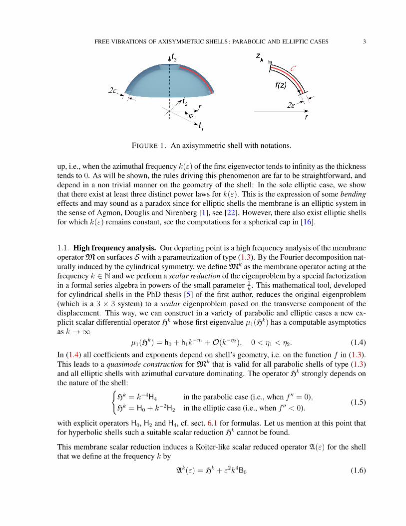
Similarly to the aforementioned publications, we consider here axisymmetric shells whose mid-surface S is parametrized by a smooth positive function f representing the radius as a function ofthe axial variable (see Figure 1):
F : I × T −→ S(z, ϕ) 7−→ (f(z) cosϕ, f(z) sinϕ, z).
(1.3)
Here I is a bounded interval and T is the torus R/2πZ. We focus on cases when sensitivity shows
FREE VIBRATIONS OF AXISYMMETRIC SHELLS : PARABOLIC AND ELLIPTIC CASES 3
FIGURE 1. An axisymmetric shell with notations.
up, i.e., when the azimuthal frequency k(ε) of the first eigenvector tends to infinity as the thicknesstends to 0. As will be shown, the rules driving this phenomenon are far to be straightforward, anddepend in a non trivial manner on the geometry of the shell: In the sole elliptic case, we showthat there exist at least three distinct power laws for k(ε). This is the expression of some bendingeffects and may sound as a paradox since for elliptic shells the membrane is an elliptic system inthe sense of Agmon, Douglis and Nirenberg [1], see [22]. However, there also exist elliptic shellsfor which k(ε) remains constant, see the computations for a spherical cap in [16].
1.1. High frequency analysis. Our departing point is a high frequency analysis of the membraneoperator M on surfaces S with a parametrization of type (1.3). By the Fourier decomposition nat-urally induced by the cylindrical symmetry, we define Mk as the membrane operator acting at thefrequency k ∈ N and we perform a scalar reduction of the eigenproblem by a special factorizationin a formal series algebra in powers of the small parameter 1
k. This mathematical tool, developed
for cylindrical shells in the PhD thesis [5] of the first author, reduces the original eigenproblem(which is a 3 × 3 system) to a scalar eigenproblem posed on the transverse component of thedisplacement. This way, we can construct in a variety of parabolic and elliptic cases a new ex-plicit scalar differential operator Hk whose first eigenvalue µ1(Hk) has a computable asymptoticsas k →∞
µ1(Hk) = h0 + h1k−η1 +O(k−η2), 0 < η1 < η2. (1.4)
In (1.4) all coefficients and exponents depend on shell’s geometry, i.e. on the function f in (1.3).This leads to a quasimode construction for Mk that is valid for all parabolic shells of type (1.3)and all elliptic shells with azimuthal curvature dominating. The operator Hk strongly depends onthe nature of the shell:
Hk = k−4H4 in the parabolic case (i.e., when f ′′ = 0),Hk = H0 + k−2H2 in the elliptic case (i.e., when f ′′ < 0).
(1.5)
with explicit operators H0, H2 and H4, cf. sect. 6.1 for formulas. Let us mention at this point thatfor hyperbolic shells such a suitable scalar reduction Hk cannot be found.
This membrane scalar reduction induces a Koiter-like scalar reduced operator A(ε) for the shellthat we define at the frequency k by
Ak(ε) = Hk + ε2k4B0 (1.6)
4 MARIE CHAUSSADE-BEAUDOUIN, MONIQUE DAUGE, ERWAN FAOU, AND ZOHAR YOSIBASH
where the function B0 is positive and explicit (k4 corresponding to the leading order in the Fourierexpansion of the bending operator B). Then we shall show that the first eigenvalue of A(ε) is theinfimum on all angular frequencies of the first eigenvalues of Ak(ε):
µ1(A(ε)) = infk∈N
µ1
(Ak(ε)
). (1.7)
In all relevant parabolic cases (i.e., cylinders and cones) and a variety of elliptic cases, we provein this paper:
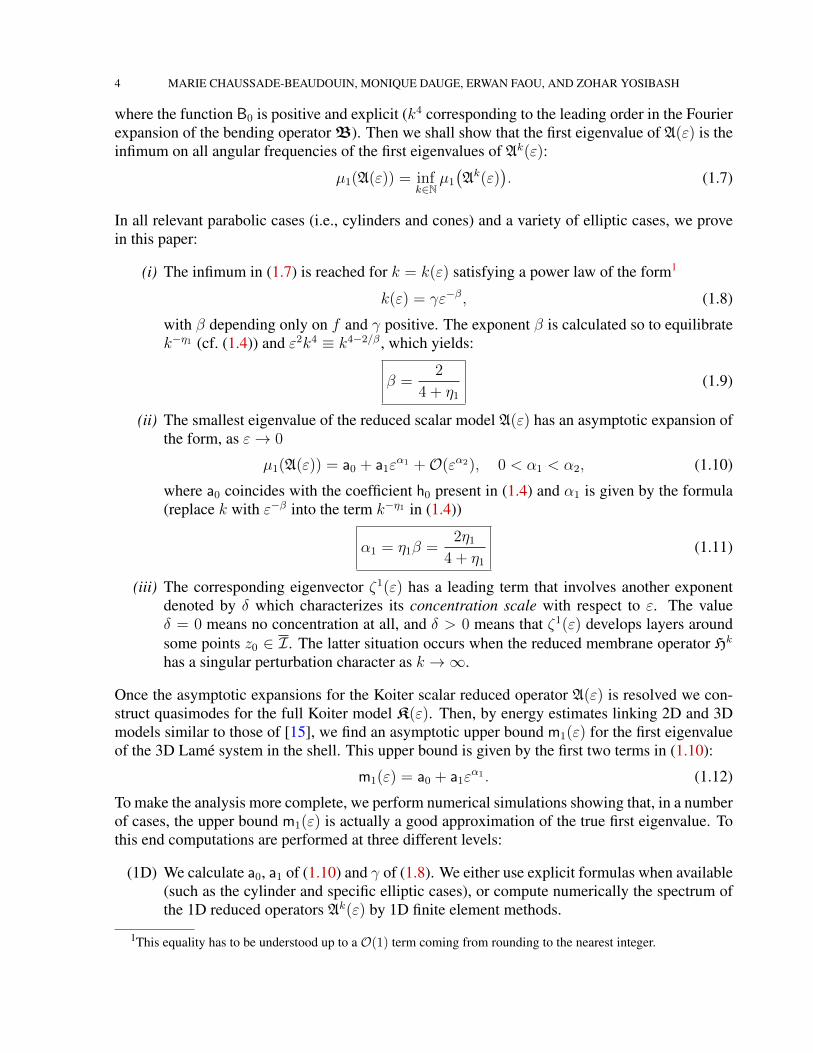
(i) The infimum in (1.7) is reached for k = k(ε) satisfying a power law of the form1
k(ε) = γε−β, (1.8)
with β depending only on f and γ positive. The exponent β is calculated so to equilibratek−η1 (cf. (1.4)) and ε2k4 ≡ k4−2/β , which yields:
β =2
4 + η1
(1.9)
(ii) The smallest eigenvalue of the reduced scalar model A(ε) has an asymptotic expansion ofthe form, as ε→ 0
µ1(A(ε)) = a0 + a1εα1 +O(εα2), 0 < α1 < α2, (1.10)
where a0 coincides with the coefficient h0 present in (1.4) and α1 is given by the formula(replace k with ε−β into the term k−η1 in (1.4))
α1 = η1β =2η1
4 + η1
(1.11)
(iii) The corresponding eigenvector ζ1(ε) has a leading term that involves another exponentdenoted by δ which characterizes its concentration scale with respect to ε. The valueδ = 0 means no concentration at all, and δ > 0 means that ζ1(ε) develops layers aroundsome points z0 ∈ I. The latter situation occurs when the reduced membrane operator Hk
has a singular perturbation character as k →∞.
Once the asymptotic expansions for the Koiter scalar reduced operator A(ε) is resolved we con-struct quasimodes for the full Koiter model K(ε). Then, by energy estimates linking 2D and 3Dmodels similar to those of [15], we find an asymptotic upper bound m1(ε) for the first eigenvalueof the 3D Lame system in the shell. This upper bound is given by the first two terms in (1.10):
m1(ε) = a0 + a1εα1 . (1.12)
To make the analysis more complete, we perform numerical simulations showing that, in a numberof cases, the upper bound m1(ε) is actually a good approximation of the true first eigenvalue. Tothis end computations are performed at three different levels:
(1D) We calculate a0, a1 of (1.10) and γ of (1.8). We either use explicit formulas when available(such as the cylinder and specific elliptic cases), or compute numerically the spectrum ofthe 1D reduced operators Ak(ε) by 1D finite element methods.
1This equality has to be understood up to a O(1) term coming from rounding to the nearest integer.
FREE VIBRATIONS OF AXISYMMETRIC SHELLS : PARABOLIC AND ELLIPTIC CASES 5
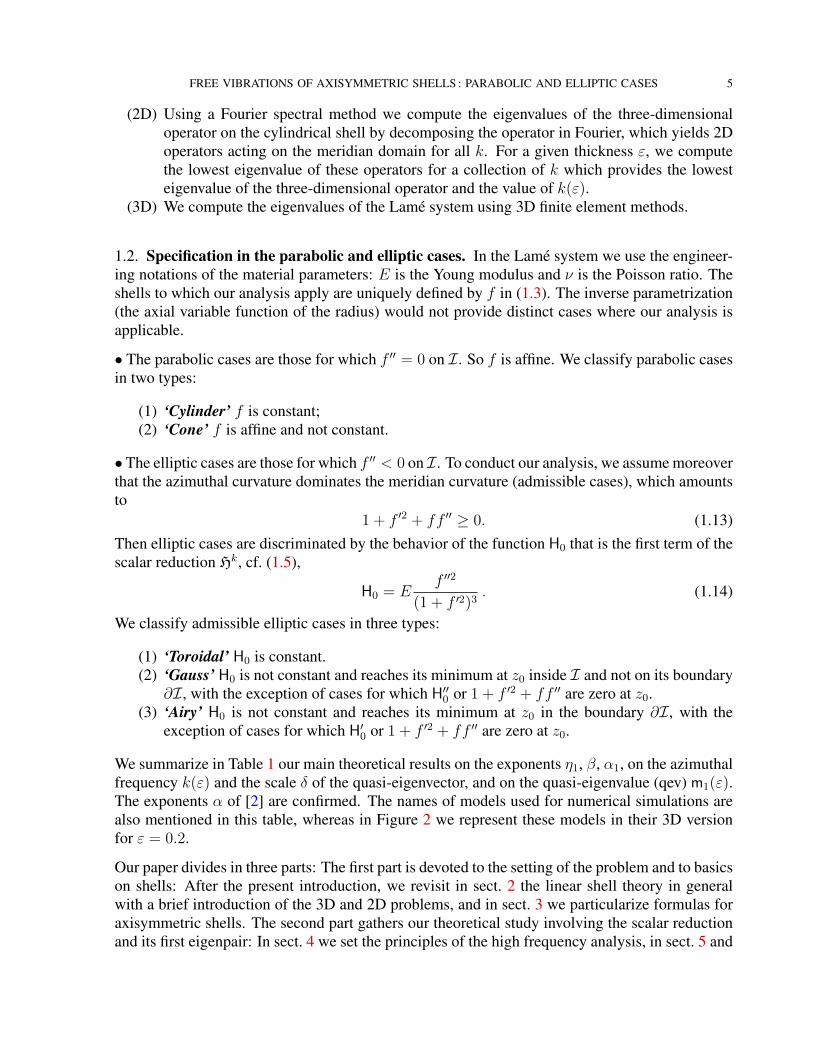
(2D) Using a Fourier spectral method we compute the eigenvalues of the three-dimensionaloperator on the cylindrical shell by decomposing the operator in Fourier, which yields 2Doperators acting on the meridian domain for all k. For a given thickness ε, we computethe lowest eigenvalue of these operators for a collection of k which provides the lowesteigenvalue of the three-dimensional operator and the value of k(ε).
(3D) We compute the eigenvalues of the Lame system using 3D finite element methods.
1.2. Specification in the parabolic and elliptic cases. In the Lame system we use the engineer-ing notations of the material parameters: E is the Young modulus and ν is the Poisson ratio. Theshells to which our analysis apply are uniquely defined by f in (1.3). The inverse parametrization(the axial variable function of the radius) would not provide distinct cases where our analysis isapplicable.
• The parabolic cases are those for which f ′′ = 0 on I. So f is affine. We classify parabolic casesin two types:
(1) ‘Cylinder’ f is constant;(2) ‘Cone’ f is affine and not constant.
• The elliptic cases are those for which f ′′ < 0 on I. To conduct our analysis, we assume moreoverthat the azimuthal curvature dominates the meridian curvature (admissible cases), which amountsto
1 + f ′2 + ff ′′ ≥ 0. (1.13)Then elliptic cases are discriminated by the behavior of the function H0 that is the first term of thescalar reduction Hk, cf. (1.5),
H0 = Ef ′′2
(1 + f ′2)3. (1.14)
We classify admissible elliptic cases in three types:
(1) ‘Toroidal’ H0 is constant.(2) ‘Gauss’ H0 is not constant and reaches its minimum at z0 inside I and not on its boundary
∂I, with the exception of cases for which H′′0 or 1 + f ′2 + ff ′′ are zero at z0.(3) ‘Airy’ H0 is not constant and reaches its minimum at z0 in the boundary ∂I, with the
exception of cases for which H′0 or 1 + f ′2 + ff ′′ are zero at z0.
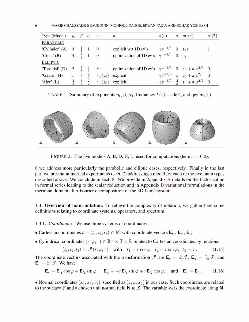
We summarize in Table 1 our main theoretical results on the exponents η1, β, α1, on the azimuthalfrequency k(ε) and the scale δ of the quasi-eigenvector, and on the quasi-eigenvalue (qev) m1(ε).The exponents α of [2] are confirmed. The names of models used for numerical simulations arealso mentioned in this table, whereas in Figure 2 we represent these models in their 3D versionfor ε = 0.2.
Our paper divides in three parts: The first part is devoted to the setting of the problem and to basicson shells: After the present introduction, we revisit in sect. 2 the linear shell theory in generalwith a brief introduction of the 3D and 2D problems, and in sect. 3 we particularize formulas foraxisymmetric shells. The second part gathers our theoretical study involving the scalar reductionand its first eigenpair: In sect. 4 we set the principles of the high frequency analysis, in sect. 5 and
6 MARIE CHAUSSADE-BEAUDOUIN, MONIQUE DAUGE, ERWAN FAOU, AND ZOHAR YOSIBASH
Type (Model) η1 β α1 a0 a1 k(ε) δ m1(ε) α [2]
PARABOLIC
‘Cylinder’ (A) 4 14 1 0 explicit wrt 1D ev’s γε−1/4 0 a1ε 1
‘Cone’ (B) 4 14 1 0 optimization of 1D ev’s γε−1/4 0 a1ε —
ELLIPTIC
‘Toroidal’ (D) 2 13
23 H0 optimization of 1D ev’s γε−1/3 0 a0 + a1ε
2/3 0
‘Gauss’ (H) 1 25
25 H0(z0) explicit γε−2/5 1
2 a0 + a1ε2/5 0
‘Airy’ (L) 23
37
27 H0(z0) explicit γε−3/7 2
3 a0 + a1ε2/7 0
TABLE 1. Summary of exponents η1, β, α1, frequency k(ε), scale δ, and qev m1(ε)
FIGURE 2. The five models A, B, D, H, L, used for computations (here ε = 0.2).
6 we address more particularly the parabolic and elliptic cases, respectively. Finally in the lastpart we present numerical experiments (sect. 7) addressing a model for each of the five main typesdescribed above. We conclude in sect. 8. We provide in Appendix A details on the factorizationin formal series leading to the scalar reduction and in Appendix B variational formulations in themeridian domain after Fourier decomposition of the 3D Lame system.
1.3. Overview of main notation. To relieve the complexity of notation, we gather here somedefinitions relating to coordinate systems, operators, and spectrum.
1.3.1. Coordinates. We use three systems of coordinates:
• Cartesian coordinates t = (t1, t2, t3) ∈ R3 with coordinate vectors Et1 , Et2 , Et3 .
• Cylindrical coordinates (r, ϕ, τ) ∈ R+ × T× R related to Cartesian coordinates by relations
(t1, t2, t3) = T (r, ϕ, τ) with t1 = r cosϕ, t2 = r sinϕ, t3 = τ . (1.15)
The coordinate vectors associated with the transformation T are Er = ∂rT , Eϕ = ∂ϕT , andEτ = ∂τT . We have
Er = Et1 cosϕ+ Et2 sinϕ, Eϕ = −rEt1 sinϕ+ rEt2 cosϕ, and Eτ = Et3 . (1.16)
• Normal coordinates (x1, x2, x3), specified as (z, ϕ, x3) in our case. Such coordinates are relatedto the surface S and a chosen unit normal field N to S. The variable x3 is the coordinate along N.
FREE VIBRATIONS OF AXISYMMETRIC SHELLS : PARABOLIC AND ELLIPTIC CASES 7
The variables (x1, x2), specified as (z, ϕ) in our case, parametrize the surface. The full transfor-mation F : (z, ϕ, x3) 7→ (t1, t2, t3) sends the product I × T × (−ε, ε) onto the shell Ωε and isexplicitly given by
t1 =(f(z) + x3
1s(z)
)cosϕ, t2 =
(f(z) + x3
1s(z)
)sinϕ, t3 = z − x3
f ′(z)s(z)
, (1.17)
where s =√
1 + f ′2. The restriction of F on the surface S (corresponding to x3 = 0) gives backF (1.3). The coordinate vectors associated with the transformation F are ∂zF =: Ez, ∂ϕT thatcoincides with Eϕ above, and ∂3F =: E3. On the surface S, x3 = 0 and E3 coincides with N,whereas Ez and Eϕ are tangent to S.
These three systems of coordinates determine the contravariant components of a displacement uin each of these systems by identities
u = ut1Et1 + ut2Et2 + ut3Et3 = urEr + uϕEϕ + uτEτ = uzEz + uϕEϕ + u3E3 . (1.18)
The cylindrical and normal systems of coordinates are suitable for angular Fourier decompositionT 3 ϕ 7→ k ∈ Z. The Fourier coefficient of rank k of a function u is denoted by uk
uk =1
2π
∫ 2π
0
u(ϕ) e−ikϕ dϕ.
For functions on Ωε, the Fourier coefficients are defined on the meridian domain ωε ⊂ R2 of Ωε.
For a 3D displacement u defined on Ωε or a surface displacement ζ defined on S, we have first toexpand them in a suitable system of coordinates (cylindric or normal) and then calculate Fouriercoefficients of their components, for instance
uk = (ur)kEr + (uϕ)kEϕ + (uτ )kEτ with (ur)k(r, τ) =1
2π
∫ 2π
0
ur(r, ϕ, τ) e−ikϕ dϕ, etc...
or
ζk = (ζz)kEz + (ζϕ)kEϕ + (ζ3)kN with (ζz)k(z) =1
2π
∫ 2π
0
ζz(z, ϕ) e−ikϕ dϕ, etc...
1.3.2. Operators. We manipulate a collection of operators and their Fourier symbols. On theshell Ωε we have the Lame system Lε acting on 3D displacements u. After angular Fourier de-composition, we obtain the family of 3×3 operators (Lε)k defined on the meridian domain ωε. Onthe surface S we have the membrane, bending and Koiter operators M, B and K(ε). They act on3-component surface displacements ζ. On the meridian curve C of S, we have the correspondingfamilies Mk, Bk and Kk(ε). Finally, on the meridian curve C, we have our scalar reductionsHk and Ak(ε) acting on functions η. We go from a higher model to a lower one by reduction,and the converse way by reconstruction. For instance we go from u to ζ by restriction to S. Theconverse way uses the reconstruction operator U (2.14). We go from ζk to ηk by selecting thenormal component of ζk. The converse way uses the reconstruction operators V[k] that we willconstruct.
1.3.3. Spectrum. We denote by σ(A) and σess(A) the spectrum and the essential spectrum of aselfadjoint operator A, respectively, which means the set of λ’s such that A − λ is not invertibleand not Fredholm, respectively.
8 MARIE CHAUSSADE-BEAUDOUIN, MONIQUE DAUGE, ERWAN FAOU, AND ZOHAR YOSIBASH
2. ESSENTIALS ON SHELL THEORY
Recall that Cartesian coordinates of a point P ∈ R3 are denoted by t = (t1, t2, t3). A shell Ωε is athree-dimensional object defined by its midsurface S and its thickness parameter ε in the followingway: We assume that S is smooth and orientable, so that there exists a smooth unit normal fieldP 7→ N(P) on S and so that for ε > 0 small enough the following map is one to one and smooth
Φ : S × (−ε, ε) → Ωε
(P, x3) 7→ t = P + x3 N(P).(2.1)
The boundary of Ωε has two parts:
(1) Its lateral boundary ∂0Ωε := Φ(∂S × (−ε, ε)
),
(2) The rest of its boundary (natural boundary) ∂1Ωε := ∂Ωε \ ∂0Ωε.
2.1. 3D vibration modes. On the domain Ωε, we consider the Lame operator associated with anisotropic and homogeneous material with Young coefficient E and Poisson coefficient ν. Thismeans that the material tensor is given by
Aijk` =Eν
(1 + ν)(1− 2ν)δijδk` +
E
2(1 + ν)(δikδj` + δi`δjk). (2.2)
For clamped boundary conditions the variational space is
V (Ωε) := u = (ut1 , ut2 , ut3) ∈ H1(Ωε)3 , u = 0 on ∂0Ωε. (2.3)
For a given displacement field u let eij(u) = 12(∂iutj + ∂juti) be the strain tensor, where ∂i stands
for the partial derivative with respect to ti. The energy scalar product between two displacementsu and u∗ is given by
aε3D(u,u∗) =
∫Ωε
Aijk`eij(u) ek`(u∗) dΩε , (2.4)
using the summation convention of repeated indices. The three-dimensional modal problem canbe written in variational form as:
Find (u, λ) in V (Ωε)× R with u 6= 0 such that
∀u∗ ∈ V (Ωε), aε3D(u,u∗) = λ
∫Ωε
utiu∗ti dΩε. (2.5)
The strong formulation of (2.5) can be written as
Lεu = λuε, (2.6)
where Lε is the Lame system
Lε = − E
2(1 + ν)(1− 2ν)
((1− 2ν)∆ +∇ div
)on Ωε, (2.7)
associated with Dirichlet BC’s on ∂0Ωε and natural BC’s on the rest of the boundary. Its spectrumσ(Lε) is discrete and positive. So its eigenvalues in (2.5) can be ordered as an increasing sequence(λεn)n≥1
0 < λε1 ≤ λε2 ≤ · · · ≤ λεn ≤ · · ·
FREE VIBRATIONS OF AXISYMMETRIC SHELLS : PARABOLIC AND ELLIPTIC CASES 9
It would be desired to obtain an asymptotic series as ε→ 0 for any chosen n ≥ 1 of λεn, at least inthe axisymmetric case. This has been realized for plates [14]:
λεn = ε2Λn +O(ε3) (2.8)
where Λn is the n-th bending eigenvalue. Presently we cannot achieve this goal in other situations.We thus concentrate on estimates for the first eigenvalue that is obtained by the minimum Rayleighquotient
λε1 = minu∈V (Ωε)
aε3D(u,u)
‖u‖2L2(Ωε)
.
In this paper we perform two tasks:
[A] Obtain asymptotic upper bounds for λε1 via the construction of quasimodes for reducedmodels and reconstruction operators,
[B] Compute numerical approximation of the smallest eigenpair in (2.5) by finite elementmethods.
2.2. 2D shell models. The 2D reduction to the midsurface S , namely the membrane and bendingoperators, are defined via intrinsic geometrical objects attached to S. To introduce them, weneed generic parametrizations F : (xα)α∈1,2 → t acting from maps neighborhoods V into themidsurface S. Associated tangent coordinate vector fields are
Eα = ∂αF , α = 1, 2, with ∂α =∂
∂xα.
Completed by the unit normal field N they form a basis E1,E2,N in each point of S. The metrictensor (aαβ) and the curvature tensor (bαβ) are given by
aαβ = 〈Eα,Eβ〉 and bαβ = 〈∂αβF ,N〉 .
Denoting by (aαβ) the inverse of (aαβ), the curvature (symmetric) matrix is defined by
(bαβ) with bαβ = aαγbγβ.
The eigenvalues κ1 and κ2 of the matrix (bαβ) are called the principal curvatures of S and theirproduct is the Gaussian curvature K. Here comes the classification of shells: If K ≡ 0, the shellis parabolic, if K > 0, the shell is elliptic, if K < 0, the shell is hyperbolic. Finally let R denotethe minimal radius of curvature of S
R = infP∈S
min|κ1(P)|−1, |κ2(P)|−1
. (2.9)
The basis Eα,N determines contravariant components (ζα, ζ3) of a vector field ζ on S:
ζ = ζtiEti = ζαEα + ζ3N .
The covariant components are (ζα, ζ3) with ζα = aαβζβ and ζ3 = ζ3. The 2D rigidity tensor on S
is given by
Mαβσδ =νE
1− ν2aαβaσδ +
E
2(1 + ν)(aασaβδ + aαδaβσ).
Note that, even if S is flat (aαβ = δαβ), M is different than the 3D rigidity tensor A.
10 MARIE CHAUSSADE-BEAUDOUIN, MONIQUE DAUGE, ERWAN FAOU, AND ZOHAR YOSIBASH
2.2.1. Membrane operator. The variational space associated with the membrane operator is
VM(S) = H10 (S)×H1
0 (S)× L2(S). (2.10)
For an element ζ = (ζα, ζ3) in VM(S), the change of metric tensor γ = γαβ(ζ) is given by
γαβ(ζ) = 12(Dαζβ + Dβζα)− bαβζ3,
where Dα is the covariant derivative on S, see [18, 19, 39]. The membrane energy scalar productis defined as
aM(ζ, ζ∗) =
∫SMαβσδγαβ(ζ) γσδ(ζ
∗) dS .
Here the volume form dS is√| det(aαβ)| dx1dx2. The variational formulation of the modal
problem associated with the membrane operator M is given by
Find (ζ,Λ) with ζ ∈ VM(S) \ 0 and Λ ∈ R such that for all ζ∗ ∈ VM(S),
aM(ζ, ζ∗) = Λ
∫S(ζβζ∗β + ζ3ζ∗3 ) dS. (2.11)
2.2.2. Bending operator and Koiter model. The variational space associated with the bendingoperator is
VB(S) = H10 (S)×H1
0 (S)×H20 (S). (2.12)
For an element ζ = (ζα, ζ3) in VB(S), the change of curvature tensor ρ = ραβ(ζ) is given by
ραβ(ζ) = DαDβζ3 + Dα(bδβζδ) + bδαDβζδ − bδαbβδζ3.
The bending operator B acts on the variational space VB(S) and its energy scalar product is
aB(ζ, ζ∗) =1
3
∫SMαβσδραβ(ζ)ρσδ(ζ
∗) dS .
For any positive ε, the Koiter operator K(ε) is defined as M + ε2B. It can be shown, see [8],that K(ε) is elliptic with multi-order on VB(S) in the sense of Agmon-Douglis-Nirenberg [1]. Thecorresponding physical energy scalar product is
aε2D(ζ, ζ∗) = 2ε aM(ζ, ζ∗) + 2ε3aB(ζ, ζ∗). (2.13)
2.3. Reconstruction operators from 2D to 3D. The parametrizations of the midsurface inducelocal system of normal coordinates (xα, x3) inside the shell and, correspondingly, the covariantcomponents uα and u3 of a displacement u. The rationale of the shell theory is to deduce by anexplicit procedure a solution u of the 3D Lame system posed on the shell from a 2D solution ζof the Koiter model posed on the midsurface. This is done via a reconstruction operator U, cf[26, 27] and [15]. With any 2D displacement ζ(xα) defined on the midsurface S, U associates a3D displacement u depending on the three coordinates (xα, x3) in Ωε. The operator U is definedby
U = T W (2.14)where W is the shifted reconstruction operator
Wζ =
ζσ − x3(Dσζ3 + bασζα),
ζ3 − ν1−ν x3 γ
αα(ζ) + ν
2−2νx2
3 ραα(ζ),
(2.15)
FREE VIBRATIONS OF AXISYMMETRIC SHELLS : PARABOLIC AND ELLIPTIC CASES 11
and T : ζ 7→ Tζ is the shifter defined as (Tζ)σ = ζσ − x3bασζα and (Tζ)3 = ζ3, see [31]. The
2D elastic energy of ζ is a good approximation of the 3D elastic energy of Uζ, cf. [15, TheoremA.1]: For any ζ ∈ (H2 ×H2 ×H3) ∩ VB(S), there holds, with non-dimensional constant A∣∣aε2D(ζ, ζ)− aε3D(Uζ,Uζ)
∣∣ ≤ Aaε2D(ζ, ζ)( εR
+ε2
L2
), (2.16)
where R is the minimal radius of curvature (2.9) of S, and L is the wave length for ζ defined asthe largest constant such that the following “inverse estimates” hold
L |γ |H1(S) ≤ ‖γ‖L2(S) and L |ρ|H1(S) ≤ ‖ρ‖L2(S) . (2.17)
Note that for ζ ∈ VB(S), the first two components of Uζ satisfy the Dirichlet condition on ∂0Ωε,whereas the third one does not need to satisfy it. In order to remedy that, we add a correctorterm ucor to Wζ to compensate for the nonzero trace g = − ν
1−ν x3 γαα(ζ) + ν
2−2νx2
3 ραα(ζ)
∣∣∂S .
This corrector term is constructed and its energy estimated in [15, sect. 7]. It has a simple tensorproduct form and exhibits the typical 3D boundary layer scale d/ε with d = dist(P, ∂0Ωε):
ucor =(
0, 0, g χ(dε
))>with χ ∈ C∞0 (R), χ(0) = 1.
“True” boundary layer terms live at the same scale, decay exponentially, but have a non-tensorform in variables (d, x3), see [17, 14] for plates and [21] for elliptic shells. Nevertheless thisexpression for ucor suffices to obtain good estimates: There holds
aε3D(ucor,ucor) ≤ Aaε2D(ζ, ζ)(ε`
+ε3
`3
),
for ` the lateral wave length of ζ defined as the largest constant such that
`|γ |2L2(∂S)
+ `3|γ |2H1(∂S)
≤ ‖γ‖2L2(S)
and `|ρ|2L2(∂S)
+ `3|ρ|2H1(∂S)
≤ ‖ρ‖2L2(S)
. (2.18)
Example 2.1. Let G in H2(R+) be such that G ≡ 0 for t ≥ 1. Let k ∈ N and 0 < τ < τ0 for τ0
small enough. The function g(z, ϕ) defined on S as
g(z, ϕ) = eikϕG(dτ
)satisfies the estimates L |g|H1(S) ≤ ‖g‖L2(S) and `|g|2L2(∂S) + `3|g|2H1(∂S) ≤ ‖g‖2
L2(S) for L and `larger than c(G) minτ, k−1 where the positive constant c(G) is independent of τ and k.
In the present work, we are interested in comparing 2D and 3D Rayleigh quotients so we introducethe following notations
Qε3D(u) =
aε3D(u,u)
‖u‖2L2(Ωε)
, and Qε2D(ζ) =
aε2D(ζ, ζ)
2ε‖ζ‖2L2(S)
.
By similar inequalities as in [15] we can prove the following relative estimate
Theorem 2.2. (i) For all ζ ∈ (H2 ×H2 ×H3) ∩ VB(S) and with U defined in (2.14) we setUζ = Uζ − ucor.
ThenUζ belongs to the 3D variational space V (Ωε). With L and ` the wave lengths (2.17) and
(2.18), let us assume ε ≤ L and ε ≤ `. We also assume Qε2D(ζ) ≤ EM for a chosen constant
12 MARIE CHAUSSADE-BEAUDOUIN, MONIQUE DAUGE, ERWAN FAOU, AND ZOHAR YOSIBASH
M ≥ 1 independent of ε. Then we have the relative estimates between Rayleigh quotients for εsmall enough ∣∣Qε
2D(ζ)−Qε3D(
Uζ)
∣∣ ≤ A′Qε2D(ζ)
( εR
+ε2
L2+(ε`
)1/2
+ ε√M), (2.19)
with a constant A′ independent of ε and ζ.
(ii) If ζ belongs to (H20 × H2
0 × H30 )(S), the boundary corrector ucor is zero and the above
estimates do not involve the term√ε/` any more.
This theorem allows to find upper bounds for the first 3D eigenvalue λε1 if we know convenientenergy minimizers ζε for the Koiter model K(ε) and if we have the relevant information abouttheir wave lengths.
3. AXISYMMETRIC SHELLS
An axisymmetric shell is invariant by rotation around an axis that we may choose as t3. Recall that(r, ϕ, τ) ∈ R+ × T × R denote associated cylindrical coordinates satisfying relations (1.15) andcoordinate vectors are Er, Eϕ, and Eτ given by (1.16). Accordingly, the (contravariant) cylindricalcomponents of a displacement u = utiEti are (ur, uϕ, uτ ) so that u = urEr + uϕEϕ + uτEτ . Inparticular the radial component of u is given by
ur = ut1 cosϕ+ ut2 sinϕ. (3.1)
The components uϕ and uτ are called azimuthal and axial, respectively.
An axisymmetric domain Ω ⊂ R3 is associated with a meridian domain ω ⊂ R+ × R so that
Ω = x ∈ R3, (r, τ) ∈ ω and ϕ ∈ T. (3.2)
3.1. Axisymmetric parametrization. For a shell Ωε that is axisymmetric, let ωε be its meridiandomain. The midsurface S of Ωε is axisymmetric too. Let C be its meridian domain. We have arelation similar to (2.1)
Φ : C × (−ε, ε) 3((r, τ), x3
)7−→ (r, τ) + x3N(r, τ) ∈ ωε. (3.3)
The meridian midsurface C is a curve in the halfplane R+ × R.
Assumption 3.1. Let I denote any bounded interval and let z be the variable in I.(i) The curve C can be parametrized by one map defined on I by a smooth function f :
I −→ Cz 7−→ (r, τ) = (f(z), z)
with f : z 7→ r = f(z). (3.4)
(ii) The shells are disjoint from the rotation axis, i.e., there exists Rmin > 0 such that f ≥ Rmin.
Remark 3.2. We impose condition (ii) to avoid technical difficulties due to the singularity at theorigin. We have observed that, if we keep this condition, the inverse parametrization z = g(r)does not bring new examples in the framework that we investigate in this paper. For instanceannular plates pertain to this inverse parametrization, but they fall in [14] that provides a completeeigenvalue asymptotics.
FREE VIBRATIONS OF AXISYMMETRIC SHELLS : PARABOLIC AND ELLIPTIC CASES 13
The parametrization (3.4) of the meridian curve C provides a parametrization of the meridiandomain ωε by I × (−ε, ε): Let us introduce the arc-length
s(z) =√
1 + f ′(z)2, z ∈ I . (3.5)
The unit normal vector N to C at the point (r, τ) = (f(z), z) is given by ( 1s(z)
,−f ′(z)s(z)
) and theparametrization by
I × (−ε, ε) 3 (z, x3) 7−→(f(z) + x3
1s(z)
, z − x3f ′(z)s(z)
)∈ ωε .
The parametrization (3.4) also induces the parametrization F (1.3) of the midsurface S by thevariables (z, ϕ) ∈ I × T. The unit normal vector N to S at the point F (z, ϕ) is given by
N = s(z)−1(Er − f ′(z)Eτ )
while tangent coordinate vectors are Ez = ∂zF and Eϕ = ∂ϕF , i.e.
Ez = f ′(z)Er + Eτ
while Eϕ coincides the coordinate vector of same name corresponding to cylindrical coordinates(1.16). The metric tensor (aαβ) is given by 〈Eα,Eβ〉 with α, β ∈ z, ϕ, i.e.(
azz azϕ
aϕz aϕϕ
)(z) =
(s(z)2 0
0 f(z)2
). (3.6)
The curvature tensor and Gaussian curvature K are respectively given by(bzz bzϕbϕz bϕϕ
)(z) =
(f ′′(z)s(z)−3 0
0 −f(z)−1s(z)−1
)and K(z) = − f ′′(z)
f(z)s(z)4. (3.7)
So the curvature tensor is in diagonal form, and K is simply the product of its diagonal elements.
Definition 3.3. We call bzz the meridian curvature and bϕϕ the azimuthal curvature.
Since we have assumed that f ≥ R0 > 0, all terms are bounded and we find that
(1) If f ′′ ≡ 0, i.e. f is affine, the shell is (nondegenerate) parabolic. If f is constant, the shellis a cylinder, if not it is a truncated cone (without conical point!).
(2) If f ′′ < 0, the shell is elliptic.(3) If f ′′ > 0, the shell is hyperbolic.
3.2. 2D axisymmetric models in normal coordinates. Relations (1.3) and (2.1) define normalcoordinates (z, ϕ, x3) in the thin shell Ωε. For example when the midsurface S is a cylinder (fconstant), the normal coordinates are a permutation of standard coordinates: (z, ϕ, x3) = (τ, ϕ, r).The associate (contravariant) decomposition of surface displacement fields ζ is written as ζ =ζzEz + ζϕEϕ + ζ3N, where ζ3 is the component of the displacement in the normal direction Nto the midsurface, ζz and ζϕ the meridian and azimuthal components respectively, defined so thatthere holds
ζt1Et1 + ζt2Et2 + ζt3Et3 = ζzEz + ζϕEϕ + ζ3N .
14 MARIE CHAUSSADE-BEAUDOUIN, MONIQUE DAUGE, ERWAN FAOU, AND ZOHAR YOSIBASH
Note that the azimuthal component is the same as defined by cylindrical coordinates. The covari-ant components are
ζz = s2ζz, ζϕ = f 2ζϕ, and ζ3 = ζ3.
The change of metric tensor γαβ(ζ) has the expression in normal coordinates
γzz(ζ) = ∂zζz −f ′f ′′
s2ζz −
f ′′
sζ3
γzϕ(ζ) =1
2(∂zζϕ + ∂ϕζz)−
f ′
fζϕ
γϕϕ(ζ) = ∂ϕζϕ +ff ′
s2ζz +
f
sζ3 ,
(3.8)
while the change of curvature tensor ραβ(ζ) is written as
ρzz(ζ) = ∂2zζ3 −
f ′′2
s4ζ3 +
2f ′′
s3∂zζz +
f ′′′s2 − 5f ′f ′′2
s5ζz
ρϕϕ(ζ) = ∂2ϕζ3 −
1
s2ζ3 −
2
fs∂ϕζϕ −
2f ′
s3ζz
ρzϕ(ζ) = ∂zϕζ3 +f ′′
s3∂ϕζz −
1
fs∂zζϕ +
2f ′
f 2sζϕ .
(3.9)
4. PRINCIPLES OF CONSTRUCTION: HIGH FREQUENCY ANALYSIS
The construction is based on the following postulate:
Postulate 4.1. The eigenmodes associated with the smallest vibrations are strongly oscillating inthe angular variable ϕ and this oscillation is dominating.
This means that if this postulate happens to be true for certain families of shells, our constructionwill provide rigorous quasimodes and, moreover, these quasimodes are candidates to be associatedwith lowest energy eigenpairs.
We may notice that Postulate 4.1 is wrong for planar shells. But it appears to be true for nonde-generate parabolic shells and some subclasses of elliptic shells.
4.1. Angular Fourier decomposition. We can perform a discrete Fourier decomposition in theshell Ωε ≡ ωε×T and in its midsurface S ≡ C ×T ∼= I ×T. For a function u(z, ϕ) in L2(I ×T)we denote its Fourier coefficients by
uk(z) =1
2π
∫ 2π
0
u(z, ϕ) e−ikϕ dϕ, k ∈ Z, z ∈ I.
This Fourier decomposition diagonalizes any operator L with coefficient independent of ϕ withrespect to the angular modes eikϕ, k ∈ Z, due to the relation:
(Lu)k = Lkuk.
Here the operators of interest are the Lame system Lε written in normal components, togetherwith the membrane and bending operators M and B defined on the spaces VM(S) and VB(S),
FREE VIBRATIONS OF AXISYMMETRIC SHELLS : PARABOLIC AND ELLIPTIC CASES 15
composing the Koiter operator K(ε). We denote by (Lε)k, Mk, Bk and Kk(ε), k ∈ Z, theangular Fourier decomposition of Lε, M, B and K(ε), respectively.
The (non decreasing) collections of the eigenvalues λε,kj of (Lε)k for all k ∈ Z gives back alleigenvalues of Lε. Note that since Lε is real valued, the eigenvalues for k and −k are identical.Thus λε1 = infk∈N λ
ε,k1 and we denote by k(ε) the smallest natural integer k such that (if exists)
λε1 = λε,k(ε)1 .
Postulate 4.1 means that k(ε)→∞ as ε→ 0.
4.2. High frequency analysis of the membrane operator. The eigenmode membrane equation(2.11) at azimuthal frequency k takes the form
Mkζk = ΛkAζk (4.1)
where A is the mass matrix
A =
azz 0 0
0 aϕϕ 0
0 0 1
=
s−2 0 0
0 f−2 0
0 0 1
. (4.2)
We construct quasimodes for Mk as k → ∞, i.e. pairs (Λk, ζk) with ζk in the domain of theoperator Mk and satisfying the estimates
‖(Mk − Λk) ζk‖L2(S) ≤ δ(k)‖ζk‖L2(S) with δ(k)/Λk → 0 as k →∞.
Now we consider the membrane operator as a formal series with respect to k
Mk = k2M0 + kM1 + M2 ≡M[k], with M[k] = k2∑n∈N
k−nMn , (4.3)
and try to solve (4.1) in the formal series algebra:
M[k]ζ[k] = Λ[k]Aζ[k]. (4.4)
Here the multiplication of formal series is the Cauchy product: For two formal series a[k] =∑n k−nan and b[k] =
∑n k−nbn, the coefficients of the series a[k] b[k] =
∑n k−ncn are given by
cn =∑
`+m=n a`bm.
The director M0 of the series M[k] is given in parametrization r = f(z) by
M0 =E
1− ν2
1−ν
2f2s20 0
0 1f4
0
0 0 0
. (4.5)
Its kernel is given by all triples ζ of the form (0, 0, ζ3)>. This is the reason why we look fora reduction of the eigenvalue problem for M to a scalar eigenvalue problem set on the normalcomponent ζ3. The key is a factorization process in the formal series algebra proved in [5, Chap.3],
M[k]V[k]− Λ[k]AV[k] = V0 (H[k]− Λ[k]) . (4.6)
16 MARIE CHAUSSADE-BEAUDOUIN, MONIQUE DAUGE, ERWAN FAOU, AND ZOHAR YOSIBASH
Here V(k) is a (formal series of) reconstruction operators whose first term V0 is the embeddingV0η = (0, 0, η)> in the kernel of M0, and H[k] is the scalar reduction.
Theorem 4.2. Let be a formal series with real coefficients :
Λ[k] =∑n≥0
k−nΛn.
For n ≥ 1, there exist operators Vn,z,Vn,ϕ : C∞(I)→ C∞(I) of order n− 1, polynomial in Λj ,for j ≤ n − 3, and for n ≥ 0 scalar operators Hn : C∞(I) → C∞(I) of order n, polynomial inΛj , for j ≤ n− 2 such that if we set :
V[k] =∑n≥0
k−nVn with Vn = (Vn,z,Vn,ϕ, 0)>, and H[k] =∑n≥0
k−nHn
we have (4.6) in the sense of formal series.
See Appendix A for more details on this theorem.
With the scalar reduction H[k] is associated the formal series problem
H[k]η[k] = Λ[k]η[k] (4.7)
where η[k] =∑
n≥0 k−nηn is a scalar formal series. The previous theorem shows that any solution
to (4.7) provides a solution ζ[k] = V[k]η[k] to (4.4).
The cornerstone of our quasimodes construction for Mk as k →∞ is to construct a solution η[k]of the problem (4.7). This relies on the possibility to extract an elliptic operator Hk with compactresolvent from the first terms of the series H[k] as we describe in several geometrical situationslater on.
Remark 4.3. The essential spectrum σess(Mk) of the membrane operator Mk at frequency k
can be determined explicitly thanks to [4, Th.4.5]. It depends only on its principal part, whichcoincides with the (multi-degree) principal part of M2, and is given by the range of E
f(z)2s(z)2for
z ∈ I, see [5, sect. 2.7] for details. With formula (3.7), we note the relation with the azimuthalcurvature
σess(Mk) =
E bϕϕ(z)2 , z ∈ I
. (4.8)
As a consequence of Assumption 3.1, the minimum of σess(Mk) is positive.
4.3. High frequency analysis of the Koiter operator. Similar to the membrane operator M[k],the bending operator expands as
Bk = k4B0 +4∑
n=1
k4−nBn ≡ B[k],
with first term
B0 =
0 0 0
0 0 0
0 0 B0
with B0 =E
1− ν2
1
3f 4. (4.9)
FREE VIBRATIONS OF AXISYMMETRIC SHELLS : PARABOLIC AND ELLIPTIC CASES 17
We notice that we have the commutation relation
B0V[k] = V0B0 .
Therefore the identity (4.6) implies for all ε the identity(M[k] + ε2k4B0
)V[k]− Λ[k]AV[k] = V0
(H[k] + ε2k4B0 − Λ[k]
). (4.10)
Thus the same factorization as for the membrane operator will generate the quasimode construc-tions for the Koiter operator as soon as the higher order terms of Bk correspond to perturbationterms. This is related to Postulate 4.1. The identity (4.10) motivates the formula (1.6) defining thereduced Koiter operator Ak(ε) = Hk + ε2k4B0. In the following two sections we provide Ak(ε)and its lowest eigenvalues in several well defined cases.
5. NONDEGENERATE PARABOLIC CASE.
We assume in addition to Assumption 3.1
f(z) = Tz +R0, z ∈ I, with R0 > 0, T ∈ R . (5.1)
If T = 0, the corresponding surface S is a cylinder of radius R0 and the minimal radius ofcurvature R (2.9) equals to R0. So we write f = R in the cylinder case. If T 6= 0, the surface S isa truncated cone. The arc length (3.5) is s =
√1 + T 2.
5.1. Membrane scalar reduction in the parabolic case. The first terms Hn of the scalar formalseries reduction of the membrane operator have been explicitly calculated in [5] in the cylindricalcase T = 0 and have the following expression in the general parabolic case:
H0 = H1 = H2 = H3 = 0 and H4(z, ∂z) = E(f 2
s6∂4z +
6f ′f
s6∂3z +
6f ′2
s6∂2z
). (5.2)
It is relevant to notice that H4 is selfadjoint on H20 (I) with respect to the natural measure dI =
f(z)s(z) dz , since there holds⟨H4η, η
∗⟩I =
E
(1 + T 2)3
∫If(z)2 ∂2
zη ∂2zη∗ dI . (5.3)
This also proves that H4 is positive. The Dirichlet boundary conditions η = ∂zη = 0 on ∂I arethe right conditions to implement the membrane boundary condition ζα = 0 on ∂I through thereconstruction operators Vn, see (A.6) – (A.7). The eigenvalue formal series Λ[k] starts with Λ4
that is the first eigenvalue of H4:
Λ0 = Λ1 = Λ2 = Λ3 = 0 and Λ4 > 0. (5.4)
The pair (Λk, ζk)
ζk =∑
0≤n+m≤6
k−n−mVnηm and Λk = k−4Λ4 (5.5)
18 MARIE CHAUSSADE-BEAUDOUIN, MONIQUE DAUGE, ERWAN FAOU, AND ZOHAR YOSIBASH
with (Λ4, η0) an eigenpair of H4, and ηm (m = 1, . . . , 6) constructed by induction so that themembrane boundary conditions ζkα = 0 are satisfied, is a quasimode for Mk. For instance, in thecylindrical case f = R, the triple ζk takes the form
ζk =
0
0
η0
+i
k
0
Rη0
0
+1
k2
−Rη′00
η2
+i
k3
0
−νR3η′′0 +Rη2
η3
− 1
k4
(ν+2)R3η′′′0 +Rη′2
Rη3
η4
+ . . .
(5.6)and the boundary conditions are, for z ∈ ∂Iη0(z) = 0, η′0(z) = 0, η2(z) = νR2η′′0(z), η′2(z) = (ν + 2)R2η′′′0 (z), η3(z) = 0, . . . (5.7)
Recall that the minimum of the essential spectrum of Mk is positive by Remark 4.3. For |k| largeenough, Mk has therefore at least an eigenvalue ∼= Λ4k
−4 under its essential spectrum and
dist(k−4Λ4, σ(Mk)
). k−5, k →∞. (5.8)
5.2. Koiter scalar reduction in the parabolic case. The leading term of the series H(k) is Hk =k−4H4, as mentioned in the introduction, see (1.5). So, the leading term of the scalar reduction ofthe Koiter operator is, cf. (4.10)
Ak(ε) = k−4H4 + ε2k4B0 = k−4H4 +ε2
3
E
1− ν2
k4
f 4. (5.9)
5.2.1. Optimizing k. The operator Ak(ε) is self-adjoint on H20 (I) and positive. Let µA
1 (ε, k) beits smallest eigenvalue. For any chosen ε we look for kmin = k(ε) realizing the minimum µA
1 (ε)of µA
1 (ε, k) if it exists:µA
1 (ε) = µA1 (ε, k(ε)) = min
k∈R+
µA1 (ε, k).
To “homogenize” the terms k−4 and ε2k4 let us define γ(ε) by setting
γ(ε) = ε1/4k(ε), (5.10)
so that we look equivalently for γ(ε). There holds
k(ε)−4H4 + ε2k(ε)4B0 = ε( 1
γ(ε)4H4 + γ(ε)4B0
).
Therefore γ(ε) does not depend on ε. Let µ1(γ) be the first eigenvalue of the operator1
γ4H4 + γ4B0 . (5.11)
The function γ 7→ µ1(γ) is continuous and, since H4 and B0 are positive, it tends to infinity as γtends to 0 or to +∞. Therefore we can define γmin as the (smallest) positive constant such thatµ1(γ) is minimum
µ1(γmin) = minγ∈R+
µ1(γ) =: a1 . (5.12)
Thus k(ε) satisfies a power law that yields a formula for the minimal first eigenvalue µA1 (ε):
k(ε) = ε−1/4γmin and µA1 (ε) = a1ε. (5.13)

FREE VIBRATIONS OF AXISYMMETRIC SHELLS : PARABOLIC AND ELLIPTIC CASES 19
5.2.2. Case of cylinders. In the cylindrical case T = 0, things are easier because f is constant.So everything can be written as a function of the first Dirichlet eigenvalue µbilap
1 of the bilaplacianoperator ∆2 on H2
0 (I) as we explain now. We have
H4 = ER2 ∆2 and B0 =E
1− ν2
1
3R4.
So the eigenvalue of 1γ4H4 + γ4B0 is
µ1(γ) =1
γ4ER2µbilap
1 + γ4 E
1− ν2
1
3R4.
It is minimum for γmin such that
γ4min = R3
√3(1− ν2)µbilap
1
and we find that the minimum eigenvalue (5.12) is
µ1(γmin) =2E
R
õbilap
1
3(1− ν2)=: a1 . (5.14)
Thusk(ε) = ε−1/4R3/4
(3(1− ν2)µbilap
1
)1/8. (5.15)
Remark 5.1. Denote by µbilap the first eigenvalue of ∆2 on the unit interval (0, 1). We have therelation µbilap
1 = µbilap L−4 with the length L of the interval I.
5.2.3. 2D reconstruction. We convert the law (5.13) giving k as a function of ε into a law givingε as a function of k
ε = k−4γ4min (5.16)
and insert it into the identity (4.10). We obtain(M[k] + γ8
mink−4B0
)V[k]− Λ[k]AV[k] = V0
(H[k] + γ8
mink−4B0 − Λ[k]
). (5.17)
So the series Λ[k] starts with the first eigenvalue Λ4 = γ4mina1 of H4 + γ8
minB0. Let η0 be anassociated eigenvector. Like before, but now with this new η0, the pair (Λk, ζk) defined by (5.5)is a quasimode for Mk + γ8
mink−4B0 = Mk + ε2k4B0 with membrane boundary conditions. To
restore the dependency on ε (via law (5.16)), we write
Λk = Λk(ε) and ζk = ζk(ε), with k = k(ε).
Since with law (5.16) the terms ε2(Bk − k4B0) are of order k−5 or higher, the same pair is aquasimode for the full Koiter operator Kk(ε), but still with membrane boundary conditions.
5.2.4. Quasimodes for the Koiter model. Bending boundary layers. The full bending boundaryconditions ζ3 = 0 and ζ ′3 = 0 on ∂I cannot be implemented in general for the quasimodes(Λk(ε), ζk(ε)). The singularly perturbed nature of the Koiter operator causes the loss of theseboundary conditions between the bending and membrane operator. Solutions of the Koiter model,just as eigenvectors, incorporate boundary layer terms. In all cases investigated in this paper, theseterms exist at the scale d/
√ε with d = dist(z, ∂I). Such a scaling appears in [33] in a variety of
nondegenerate cases (the boundary of ∂S is noncharacteristic for the curvature). It is rigorouslyanalyzed in [21] in the case of static clamped elliptic shells.
20 MARIE CHAUSSADE-BEAUDOUIN, MONIQUE DAUGE, ERWAN FAOU, AND ZOHAR YOSIBASH
More precisely, the scaled variable is (for I = (z−, z+))
Z =d√ε
with d = z+ − z or z − z−, (5.18)
according as we consider the localization at the end z0 = z+ or z0 = z− of the interval I. In viewof law (5.13), we can write the operator Kk(ε) as a series in powers of ε1/4. In the rapid variable Z,there holds ∂zG(Z) = ε−1/2G′ for any profile G(Z), which provides a new formal series K[ε1/4].Its leading term K0 is compatible with the full bending boundary conditions at Z = 0. It has thefollowing form in the cylindrical case f = R
K0 =E
1− ν2
−∂2Z 0 ν
R∂Z
0 −1−ν2R2 ∂
2Z 0
− νR∂Z 0 1
R2 + 13∂4Z
.
It allows to construct a series of exponentially decreasing vector functions G[ε1/4] satisfying a for-mal series relation of the type K[ε1/4]G[ε1/4] = Λ[ε1/4]G[ε1/4], that compensate for the missing
traces of ζk(ε), see [5, Section 5.6]. Our “true” quasimode has now the form (Λk(ε),ζk(ε)) with
ζk(ε)(z) = ζk(ε)(z) + χ(d)
6∑n=2
εn/4Gn(Z) with the same Λk(ε) = µA1 (ε) = a1ε . (5.19)
Here χ is a smooth cut-off that localizes near the boundary ∂I. The outcome is the spectralestimate
dist(a1ε , σ(Kk(ε))
). ε5/4 with k(ε) = ε−1/4γmin, as ε→ 0. (5.20)
5.3. 3D reconstruction and Rayleigh quotients. We construct a three-component vector fieldon the surface S by setting in normal coordinates
ζε(z, ϕ) = eikϕζk(z) with ζk given in (5.19) and k = k(ε) = ε−1/4γmin.
By construction, ζε belongs to the variational space VB(S), and by the elliptic regularity of theKoiter problem, it also belongs to (H2 × H2 × H3)(S). So we may apply the reconstructionoperator introduced in Theorem 2.2: Set
uε =Uζε.
To take advantage of the comparison (2.19) between the Rayleigh quotients of ζε and uε, we haveto exhibit the behavior of the wave lengths L = Lε (2.17) and ` = `ε (2.18) of ζε as ε → 0.Following the construction of the fields ζε, we see that they all originate from an eigenfunction η0
that does not depend on ε. The nontrivial behavior of Lε and `ε arises from, cf. Example 2.1:
• The Koiter boundary layer terms Gn(Z) = Gn(d/ε1/2) that contribute a term in ε1/2,• The azimuthal oscillation eikϕ that contributes a term in k−1 ' ε1/4.
As a result we find in the nondegenerate parabolic case
Lε, `ε & ε1/2.

FREE VIBRATIONS OF AXISYMMETRIC SHELLS : PARABOLIC AND ELLIPTIC CASES 21
So the assumptions of Theorem 2.2 are uniformly satisfied for the family (ζε)ε and the estimate(2.19) reads now ∣∣Qε
2D(ζε)−Qε3D(uε)
∣∣ . ε1/4Qε2D(ζε) . ε5/4 .
Stricto sensu, we have at hand a family of 3D displacements uε with azimuthal frequency k(ε) ≡ε−1/4γmin such that ∣∣Qε
3D(uε)− a1ε∣∣ . ε5/4.
Moreover the trace of the transverse component uε3 on the midsurface (x3 = 0) is close to thegenerating eigenvector η0. We have proved the results summarized in the first two lines of Table1. Our numerical experiments (Model A, sect. 7.1, and Model B, sect. 7.2) suggest that, in fact,(a1ε,uε) is an approximation of the first 3D eigenpair.
6. ELLIPTIC CASE (SMALL MERIDIAN CURVATURE)
The elliptic case in parametrization r = f(z), z ∈ I, corresponds to the situation f ′′ < 0 on I.
6.1. Membrane reduction in the general case. When the parametrizing function f is not affine,i.e., when f ′′ 6≡ 0, the scalar reduction of the membrane operator has non-vanishing first terms asfollows:
H0(z, ∂z) = Ef ′′2
s6, H1(z, ∂z) = 0, H2(z, ∂z) = H
(2)2 (z) ∂2
z + H(1)2 (z) ∂z + H
(0)2 (z) (6.1)
with
H(2)2 (z) = 2E
(ff ′′s6
+f 2f ′′2
s8
)H
(1)2 (z) = 2E
(2f ′f ′′
s6+ff ′′′
s6− 2ff ′f ′′2
s8+
2f 2f ′′f ′′′
s8− 7f 2f ′f ′′3
s10
)H
(0)2 (z) = E
(− 10f ′2f ′′2
s8+
4f ′f ′′′
s6+
2f ′2f ′′
fs6− (ν − 2)ff ′2f ′′3
s10− 5ff ′f ′′f ′′′
s8
+ff (4)
s6+
2f 2f ′′f (4)
s8+
36f 2f ′2f ′′4
s12+
(ν − 2)ff ′′3
s8− 6f 2f ′′4
s10
− 20f 2f ′f ′′2f ′′′
s10
)− Λ0
(1
s− νf ′′f
s3
)2
.
(6.2)
The rank-3 operator in the formal series H[k] is given by
H3(z, ∂z) =(− 1
s2+
2νff ′′
s4− ν2f 2f ′′2
s6
)Λ1, (6.3)
and the rank-4 operator can be written as
H4(z, ∂z) =4∑j=0
H(j)4 (z)∂jz , with H
(4)4 (z) = E
(4f 3f ′′
s8+
3f 4f ′′2
s10+f 2
s6
)(6.4)
where the other terms H(j)4 (z) are smooth functions of z.
22 MARIE CHAUSSADE-BEAUDOUIN, MONIQUE DAUGE, ERWAN FAOU, AND ZOHAR YOSIBASH
So, H0(z, ∂z) = H0(z) is the multiplication by a function (which can be seen as a potential) andwe check that H2 is a selfadjoint operator of order 2 on H1
0 (I) with respect to the natural measuredI = f(z)s(z) dz : ⟨
H2η, η∗⟩I =
∫I
(− H
(2)2 (z) ∂zη ∂zη
∗ + H(0)2 (z) η η∗
)dI . (6.5)
We recall from (3.7) that the principal curvatures are bzz = f ′′
s3and bϕϕ = − 1
fs. Note that both are
negative in the elliptic case.
Remark 6.1. (i) The function H0/E coincides with the square of the meridian curvature
H0 = E (bzz)2.
(ii) There holds the following relation between H(2)2 and the principal curvatures
− H(2)2 = 2E
f 2
s2bzz(b
ϕϕ − bzz). (6.6)
(iii) Similarly
H(4)4 = E
f 4
s4(bϕϕ − 3bzz)(b
ϕϕ − bzz). (6.7)
6.2. High frequency analysis of the membrane operator in the elliptic case. As mentionedabove, we have to select one or several terms starting the series H[k] that will play the role ofan engine to work out a recurrence and allow to solve the formal series problem (4.7). In theparabolic case, this engine is h4H4. In the elliptic case, H0 is the multiplication by the positivefunction E(bzz)
2. Its spectrum is essential and its bottom determines Λ0
Λ0 = Eminz∈I
(bzz)2. (6.8)
We have to complete H0 by further terms so that to obtain an operator with discrete spectrum closeto the minimum energy Λ0. This will be the case for the operator
Hk = H0 + k−2H2 (6.9)
if, cf. condition (1.13),
− H(2)2 ≥ 0 on I, i.e. |bϕϕ| ≥ |bzz| on I, (6.10)
(use (6.6)), with strict inequalities for the values of z where H0 attains its minimum Λ0. It isinteresting to note that the latter condition implies that, cf. (6.8) and (4.8),
minz∈I
(bzz)2 < min
z∈I(bϕϕ)2, i.e. Λ0 < minσess(M
k),
which means that the expected limit at high frequency will be attained by eigenvalues below theessential spectrum.
Remark 6.2. We note that in the hyperbolic case, f ′′ > 0, so bzz > 0. Hence the coefficient −H(2)2
is always negative and our analysis never applies in the hyperbolic case. Besides, in this case,Λ0 is not the membrane high frequency limit, that is indeed 0 (recall that the exponent in (1.2) isα = 2
3in hyperbolic case).
FREE VIBRATIONS OF AXISYMMETRIC SHELLS : PARABOLIC AND ELLIPTIC CASES 23
From now on, we assume that (6.10) holds and we discuss the lowest eigenpairs of the operatorsHk defined in (6.9) and
Ak(ε) = H0 + k−2H2 + ε2k4B0, where B0 =1
3
E
1− ν2
1
f 4(6.11)
in relation with properties of the “potential” H0. For simplicity we denote
g(z) := −H(2)2 (z), (6.12)
and consider successively the cases when H0 has a non-degenerate minimum inside or on theboundary of the interval I, or when it is constant.
6.3. Internal minimum of the potential (Gaussian case). Besides (6.10), we assume that H0
has a (unique) nondegenerate minimum in z0 ∈ I. Thus
Λ0 = H0(z0) and ∂2zH0(z0) > 0.
We assume moreover g(z0) > 0.
6.3.1. High frequency analysis for the membrane operator. Then the lowest eigenpairs of themembrane reduction Ak = H0 + k−2H2 as k →∞ are driven by the harmonic oscillator
− g(z0) ∂2Z +
Z2
2∂2zH0(z0) . (6.13)
Here, the new homogenized variable Z spans R and is linked to the physical variable z by therelation
Z =√k (z − z0) . (6.14)
This change of variable can be applied to the formal series reduction (4.6) as follows: Let L[k] =∑k≥0 k
−nLn(z, ∂z) be a formal series such that Ln is an operator of order n. By Taylor expan-sion around z0, we can expand for all n the operator Ln(z, ∂z) =
∑j≥−n k
−j/2Ln,j(Z, ∂Z). Byreordering the powers of k−j/2, we thus see that we can write
L[k] ≡ L[k1/2] =∑n≥0
k−n/2Ln(Z, ∂Z),
where the operators Ln have polynomial coefficients in Z. Applying this change of variable to theformal series reduction given in Theorem 4.2, we obtain the new identity
M[k1/2]V [k1/2]− Λ[k1/2]AV [k1/2] = V0 (H[k1/2]− Λ[k1/2]) , (6.15)
where M[k1/2], V [k1/2] and H[k1/2] are the formal series induced by the formal series M[k],V[k] and H[k] respectively. We also agree that Λ[k1/2] is related with the old series Λold[k] =∑
n≥0 k−nΛn,old by the identities Λn = 0 if n is odd, and Λn = Λn/2,old if n is even. Moreover, we
calculate that
H0 = H0(z0), H1 = 0, and H2 = −g(z0) ∂2Z +
Z2
2∂2zH0(z0).
Like for (4.7), the previous reduction leads to consider the formal series problem
H[k1/2]η[k1/2] = Λ[k1/2]η[k1/2] . (6.16)
24 MARIE CHAUSSADE-BEAUDOUIN, MONIQUE DAUGE, ERWAN FAOU, AND ZOHAR YOSIBASH
The first equation induced by this identity is H0η0 = Λ0η0, hence we have found again Λ0 =H0 = H0(z0). Since for any η we have nowH0η = Λ0η, the next equations yield
H1η0 = Λ1η0 and H2η0 = Λ2η0.
Therefore Λ1 = 0 (which is coherent with what was agreed in identity (6.15)) and η0 is an eigen-vector of the harmonic oscillator (6.13). The eigenvalues of this latter operator are
(2`− 1) c , ` = 1, 2, . . . with c =1√2
√g(z0) ∂2
zH0(z0) (6.17)
and the corresponding eigenvectors are Gaussian functions. Taking η0(Z) as the first eigenmode(` = 1) we can construct the first terms η1, η2, . . . of the formal series problem (6.16). As the coef-ficients of the operators Hj depend polynomially on Z, these terms are exponentially decreasingwith respect to Z. We can then define the pair (Λk, ζk) by the formula
ζk = χ(z)(V0η0 +
∑1≤n+m≤6
k−(n+m)/2(Vnηm)(√k(z − z0))
)Λk = H0(z0) + k−1c ,
(6.18)
where χ ∈ C∞0 (I) is identically equal to 1 in a neighborhood of z0. This pair is a quasimode forthe full membrane operator Mk as k →∞, and we obtain that
dist(H0(z0) + k−1c , σ(Mk)
). k−3/2, k →∞. (6.19)
Note that in this case, the boundary conditions are automatically fulfilled as the quasimode con-structed is localized near z0.
6.3.2. High frequency analysis for Koiter and Lame operators. Now we consider the operatorAk(ε) defined in (6.11). We look for its smallest eigenvalue µA
1 (ε, k) and for each ε > 0 smallenough, look for k(ε) such that µA
1 (ε, k(ε)) is minimum. Setting δ := ε2k4, we see that theoperator Ak(ε) has the form
W + k−2H2 with W = H0 + δB0.
If δ is small enough, the function W has the same property as H0, i.e., it has a (unique) nonde-generate minimum. Let z0(δ) be the point where this minimum is attained. By implicit functiontheorem, the correspondence δ → z0(δ) is smooth for δ small enough and there holds
µA1 (ε, k) = H0(z0(δ)) + δB0(z0(δ)) +
k−1
√2
√g(z0(δ)) ∂2
z (H0 + δB0)(z0(δ)) +O(k−3/2)
ButH0(z0(δ)) = H0(z0) +O(δ2), ∂2
zH0(z0(δ)) = ∂2zH0(z0) +O(δ),
B0(z0(δ)) = B0(z0) +O(δ), g(z0(δ)) = g(z0) +O(δ).
Hence
µA1 (ε, k) = H0(z0) + δB0(z0) +
k−1
√2
√g(z0) ∂2
zH0(z0) +O(δ2) +O(k−1δ) +O(k−3/2).
Let us set
b = B0(z0) and c =1√2
√g(z0) ∂2
zH0(z0) . (6.20)
FREE VIBRATIONS OF AXISYMMETRIC SHELLS : PARABOLIC AND ELLIPTIC CASES 25
So, replacing δ by its value ε2k4, we look for k = k(ε) such that ε2k4b + k−1c is minimum andsuch that δ = ε2k4 is small2. We homogenize the powers of k by letting γ(ε) = k(ε) ε2/5, andsetting µA
1 (ε) = µA1 (ε, k(ε)) we find
k(ε) = γ ε−2/5 and µA1 (ε) = H0(z0) + a1 ε
2/5 +O(ε3/5), (6.21)
with the explicit constants γ and a1:
γ =( c
4b
)1/5
and a1 = (4bc4)1/5(1 +1
4) . (6.22)
Along the same lines as in the parabolic case, we convert the power law for k (6.21) into thepower law ε = (γ/k)5/2. We can then consider a formal series reduction as in (5.17) and combineit with the change of variable Z =
√k(z − z0). The same analysis as before yields quasimodes
(Λk(ε), ζk(ε)). Here Λk(ε) = µA1 (ε) and ζk(ε) has a form similar to (6.18), whereas k = k(ε).
Note that these quasimodes remain localized around z0 and hence bending boundary layers do notshow up as they did in the parabolic case. We thus obtain
dist(m1(ε) , σ(K(ε))
). ε3/5 with m1(ε) = H0(z0) + a1 ε
2/5. (6.23)
Remark 6.3. If H0 attains its minimum a0 in a finite number of points z(i)0 , we can construct
quasimodes attached to each of these points of the same form as above, and with disjoint supports.The associated quantities obey to the same formulas as in (6.21)-(6.23)
k(i)(ε) = γ(i) ε−2/5 and m(i)1 (ε) = a0 + a
(i)1 ε2/5,
with γ(i) and a(i)1 defined by (6.22) with the values of quantities b and c at point z(i)
0 . Thenm1(ε) = minim
(i)1 (ε) and k(ε) = k(i0)(ε) for i0 such that the previous minimum is attained.
6.3.3. 3D reconstruction and Rayleigh quotients. As in the parabolic case, we construct a three-component vector field on the surface S by setting in normal coordinates
ζε(z, ϕ) = eikϕζk(z) with ζk given in (6.18) and k = ε−2/5γmin,
and by setting
uε =Uζε.
Since all traces of any order of ζε vanish on ∂I, there is no boundary corrector and we are in case(ii) of Theorem 2.2. So we only have to estimate the behavior of the wave length L = Lε (2.17)of ζε as ε→ 0. We note the influence of:
• The profiles Gn(√k(z − z0)) with k ' ε−2/5, that contribute a term in 1/
√k ' ε1/5,
• The azimuthal oscillation eikϕ that contributes a term in k−1 ' ε2/5.
As a result we find in the nondegenerate parabolic case
Lε & ε2/5.
So the assumptions of Theorem 2.2 are uniformly satisfied for the family (ζε)ε and the estimate(2.19) reads now ∣∣Qε
2D(ζε)−Qε3D(uε)
∣∣ . εQε2D(ζε) . ε .
2We check that δ = O(ε2/5)
26 MARIE CHAUSSADE-BEAUDOUIN, MONIQUE DAUGE, ERWAN FAOU, AND ZOHAR YOSIBASH
Thus, we have exhibited a family of 3D displacements uε with azimuthal frequency k(ε) ≡ ε−2/5γsuch that ∣∣Qε
3D(uε)−m1(ε)∣∣ . ε3/5 with m1(ε) = H0(z0) + a1 ε
2/5.
So we have proved the results summarized in the third line of Table 1. The numerical experiments(Model H, sect. 7.4) suggest that (m1(ε),uε) is indeed an approximation of the first 3D eigenpair.
6.4. Minimum of the potential on the boundary (Airy case). We assume that H0 attains itsminimum at a point z0 ∈ ∂I with ∂zH0(z0) 6= 0. Let us agree that z0 is the left end of I, i.e.,z0 = z−, so that we have
Λ0 = H0(z0) and ∂zH0(z0) > 0.
We still assume g(z0) > 0. The analysis is somewhat similar to the previous case, though a littlemore tricky.
6.4.1. High frequency analysis for the membrane operator. Membrane boundary layers. We meetthe Airy-like operator
− g(z0)∂2Z + Z ∂zH0(z0) (6.24)
on H10 (R+) instead the harmonic oscillator (6.13). The homogenized variable Z is given by
Z = (z − z0)k2/3. (6.25)
We can perform an analysis very similar to the previous case by doing a change of variable in theformal series reduction. This yields formal series problem in powers of k−1/3 whose first termsare given byH0 + k−2/3H2 whereH0 = H0(z0) andH2 is the operator (6.24). The eigenvalues ofthe model operator (6.24) are given by
z(`)Airy
(g(z0)
)1/3 (∂zH0(z0)
)2/3, ` = 1, 2, . . . (6.26)
where z(`)Airy is the `-th zero of the reverse Airy function Ai. We find that the first eigenvalue of the
membrane reduction Hk satisfies
µH1 (k) = H0(z0) + k−2/3c +O(k−1) with c = z
(1)Airy
(g(z0)
)1/3 (∂zH0(z0)
)2/3. (6.27)
Using the reconstruction operators V [k1/3] in the scaled variable allows to construct displacementζk from an eigenfunction profile η0(Z) of the Airy operator. However, the first terms of thereconstruction take the form:k
−4/3ζkzk−1ζkϕζk3
where
ζkz
ζkϕζk3
=
f2(bϕϕ − (ν + 2)bzz)∂Zη0
−if 2(bϕϕ + νbzz)η0
η0
+O(k−1/3) .
While we can impose η0(0) = 0 to ensure that ζkϕ = 0 at first order, we see that we have in generalζkz 6= 0. To construct a quasimode, we have to add new boundary layer terms to ζk.
To determine such boundary layers near z0 = z−, we introduce the scaled variable Z = kd withd = z−z−. Like already seen for the Koiter operator (sect. 5.2.4), the formal series operator M[k]
FREE VIBRATIONS OF AXISYMMETRIC SHELLS : PARABOLIC AND ELLIPTIC CASES 27
is changed to a new formal series M [k] whose first term is given by
M 0 =
−1s4∂2Z + 1−ν
2(bϕϕ)2 −1+ν
2i(bϕϕ)2∂Z
1s2
(bzz + νbϕϕ)∂Z
−1+ν2i(bϕϕ)2∂Z −1−ν
2(bϕϕ)2∂2
Z + 1f4
i 1f2
(bϕϕ + νbzz)
− 1s2
(bzz + νbϕϕ)∂Z −i 1f2
(bϕϕ + νbzz) (bϕϕ + νbzz)2
where the quantities are evaluated in z0 = z−. We can prove that this operator yields boundarylayer profiles G(Z) exponentially decreasing with respect to Z = kd, and satisfying Gz(0) = azfor any given number az, which allows to compensate for the trace of the first term of ζkz .
We obtain a compound quasimode combining terms at scale k2/3d and terms at scale kd, anddeduce in the end
dist(H0(z0) + k−2/3c , σ(Mk)
). k−1, k →∞. (6.28)
6.4.2. High frequency analysis for Koiter operator. The Koiter scalar reduction operator Ak(ε),see (6.11) is still an Airy-like operator because the minimum of H0 + ε2k4 is still z0 for ε2k4 smallenough. We look for k = k(ε) such that ε2k4b + k−2/3c is minimum. We homogenize ε2k4 withk−2/3. We find
k(ε) = γ ε−3/7 and µA1 (ε) = H0(z0) + a1 ε
2/7 +O(ε3/7), (6.29)
with the explicit constants γ and a1, with b = B0(z0) and c defined in (6.27):
γ =( c
6b
)3/14
and a1 = (6bc6)1/7(1 +1
6) . (6.30)
Note that in this case, two types of boundary layer terms are present: the one constructed above(membrane boundary layer) and the bending boundary layers terms associated with the Koiteroperator, see sect. 5.2.4. We obtain
dist(m1(ε) , σ(K(ε))
). ε3/7 with m1(ε) = H0(z0) + a1 ε
2/7.
At this point, the reconstruction operatorU is not precise enough to allow us to conclude as in the
parabolic and Gaussian cases. Nevertheless numerical experiments (Model L, sect. 7.5) tend toconfirm that the first eigenvalue of the Lame operator Lε behaves like m1(ε).
6.5. Constant potential (toroidal case). Let us assume that H0 is constant. We recall that H0 =E(bzz)
2. But bzz coincides with the curvature of the arc C of equation r = f(z) in the meridianplane. So, bzz is constant if and only if C is a circular arc. Let R be its radius and (r, z) ∈ R2 beits center. Notice that the center of the circular arc may be at negative r. Then, in the elliptic casef ′′ < 0,
f(z) = r +√R2 − (z − z)2, (6.31)
and the principal curvatures are given by
bzz = − 1
Rand bϕϕ(z) = − 1
R
(1− r
f(z)
). (6.32)
So in this case, we have
H0 =E
R2= Λ0 and g = −H(2)
2 = −2Ef
s2
rR2
. (6.33)
28 MARIE CHAUSSADE-BEAUDOUIN, MONIQUE DAUGE, ERWAN FAOU, AND ZOHAR YOSIBASH
Now the Koiter scalar reduction operator Ak(ε) is H0 + k−2H2 + ε2k4B0 where H0 is a constantfunction acting as a simple shift on the spectrum. In this case, no concentration occurs, and wehave simply to come back to the approach used for the parabolic case mutatis mutandis, with k−2
instead of k−4.
6.5.1. Membrane scalar reduction. We assume the sharp version of condition (6.10) (strict in-equalities) that ensures that H2 has a compact resolvent and is semibounded from below. Thanksto (6.33), we find that such condition is equivalent to
r < 0 . (6.34)
Let Λ2 be the first eigenvalue of H2. Then the first eigenvalue of the membrane scalar reductionoperator Hk = H0 + k−2H2 is Λ0 + k−2Λ2 and we can deduce that
dist(Λ0 + k−2Λ2 , σ(Mk)
). k−5/2, k →∞. (6.35)
6.5.2. Koiter scalar reduction. The operator Ak(ε) = H0 + k−2H2 + ε2k4B0 is self-adjoint onH1
0 (I). Let µA1 (ε, k) be its first eigenvalue. For any chosen ε we look for k(ε) realizing the
minimum of µA1 (ε, k). We set
γ(ε) = k(ε) ε1/3 (6.36)so that our operator becomes
H0 + ε2/3( 1
γ(ε)2H2 + γ(ε)4 B0
).
Therefore γ does not depend on ε. Let µ1(γ) be the first eigenvalue of the operator1
γ2H2 + γ4 B0 . (6.37)
The function γ 7→ µ1(γ) is continuous. At this point we need the following extra assumption:
Λ2 > 0, i.e. H2 > 0. (6.38)
Then the same argument as in the parabolic case allows to define γmin as the (smallest) positiveconstant such that µ1(γ) is minimum
µ1(γmin) = minγ∈R+
µ1(γ) =: a1 . (6.39)
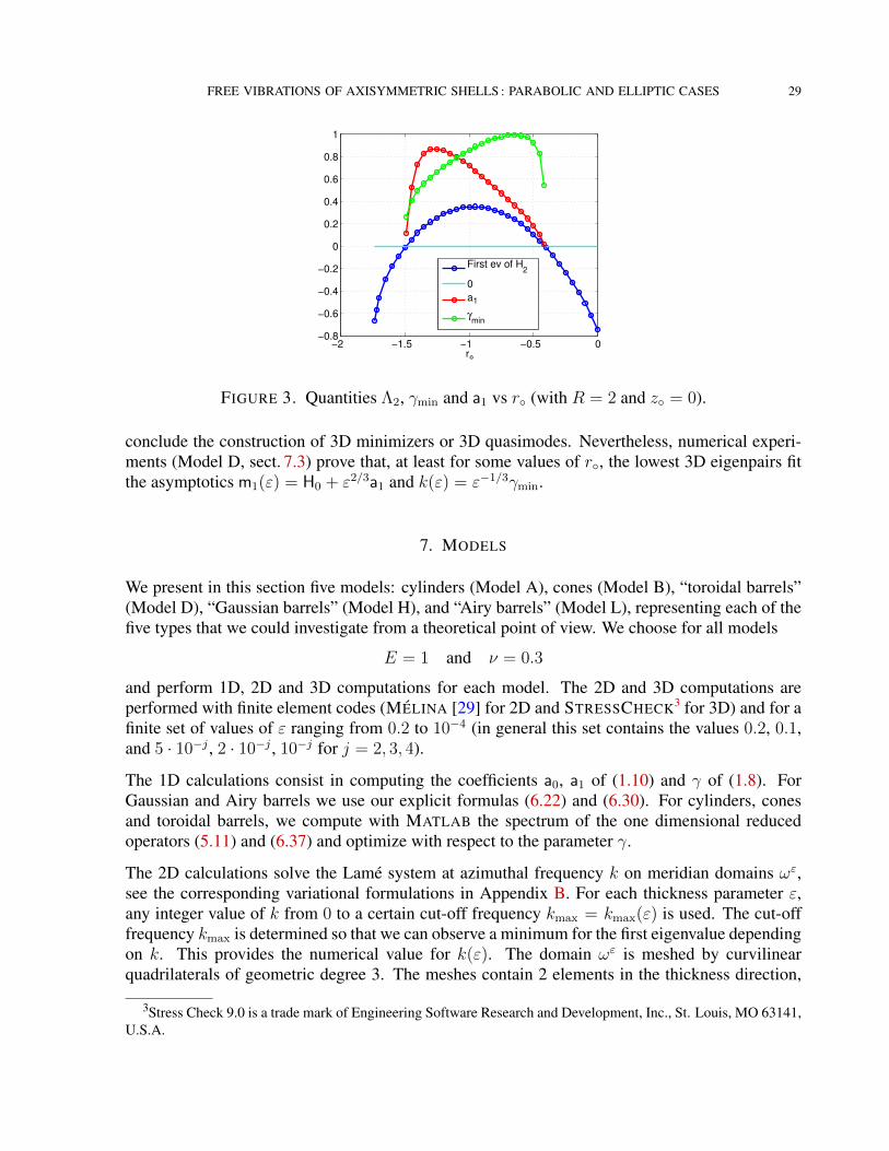
As an illustration of the non-trivial behavior of the quantities Λ2, γmin and a1, we plot them versusr in Figure 3 (we choose R = 2 and z = 0).
Thus k(ε) satisfies a power law that yields a formula for the minimal first eigenvalue µA1 (ε):
k(ε) = ε−1/3γmin and µA1 (ε) = m1(ε) = H0 + ε2/3a1 , (6.40)
and after adding membrane and bending boundary layer terms as in the Airy case we arrive to
dist(m1(ε) , σ(K(ε))
). ε with m1(ε) = H0 + ε2/3a1.
We note that, in contrast with the two previous cases when H0 is not constant, the lower order termH
(0)2 of the operator H2 is involved in the asymptotics. Finally, like in the Airy case, we would
need a more complete reconstruction operator combined with “plates” boundary layer terms to
FREE VIBRATIONS OF AXISYMMETRIC SHELLS : PARABOLIC AND ELLIPTIC CASES 29
−2 −1.5 −1 −0.5 0−0.8
−0.6
−0.4
−0.2
0
0.2
0.4
0.6
0.8
1
r°
First ev of H2
0
a1
γmin
FIGURE 3. Quantities Λ2, γmin and a1 vs r (with R = 2 and z = 0).
conclude the construction of 3D minimizers or 3D quasimodes. Nevertheless, numerical experi-ments (Model D, sect. 7.3) prove that, at least for some values of r, the lowest 3D eigenpairs fitthe asymptotics m1(ε) = H0 + ε2/3a1 and k(ε) = ε−1/3γmin.
7. MODELS
We present in this section five models: cylinders (Model A), cones (Model B), “toroidal barrels”(Model D), “Gaussian barrels” (Model H), and “Airy barrels” (Model L), representing each of thefive types that we could investigate from a theoretical point of view. We choose for all models
E = 1 and ν = 0.3
and perform 1D, 2D and 3D computations for each model. The 2D and 3D computations areperformed with finite element codes (MELINA [29] for 2D and STRESSCHECK3 for 3D) and for afinite set of values of ε ranging from 0.2 to 10−4 (in general this set contains the values 0.2, 0.1,and 5 · 10−j , 2 · 10−j , 10−j for j = 2, 3, 4).
The 1D calculations consist in computing the coefficients a0, a1 of (1.10) and γ of (1.8). ForGaussian and Airy barrels we use our explicit formulas (6.22) and (6.30). For cylinders, conesand toroidal barrels, we compute with MATLAB the spectrum of the one dimensional reducedoperators (5.11) and (6.37) and optimize with respect to the parameter γ.
The 2D calculations solve the Lame system at azimuthal frequency k on meridian domains ωε,see the corresponding variational formulations in Appendix B. For each thickness parameter ε,any integer value of k from 0 to a certain cut-off frequency kmax = kmax(ε) is used. The cut-offfrequency kmax is determined so that we can observe a minimum for the first eigenvalue dependingon k. This provides the numerical value for k(ε). The domain ωε is meshed by curvilinearquadrilaterals of geometric degree 3. The meshes contain 2 elements in the thickness direction,
3Stress Check 9.0 is a trade mark of Engineering Software Research and Development, Inc., St. Louis, MO 63141,U.S.A.
30 MARIE CHAUSSADE-BEAUDOUIN, MONIQUE DAUGE, ERWAN FAOU, AND ZOHAR YOSIBASH
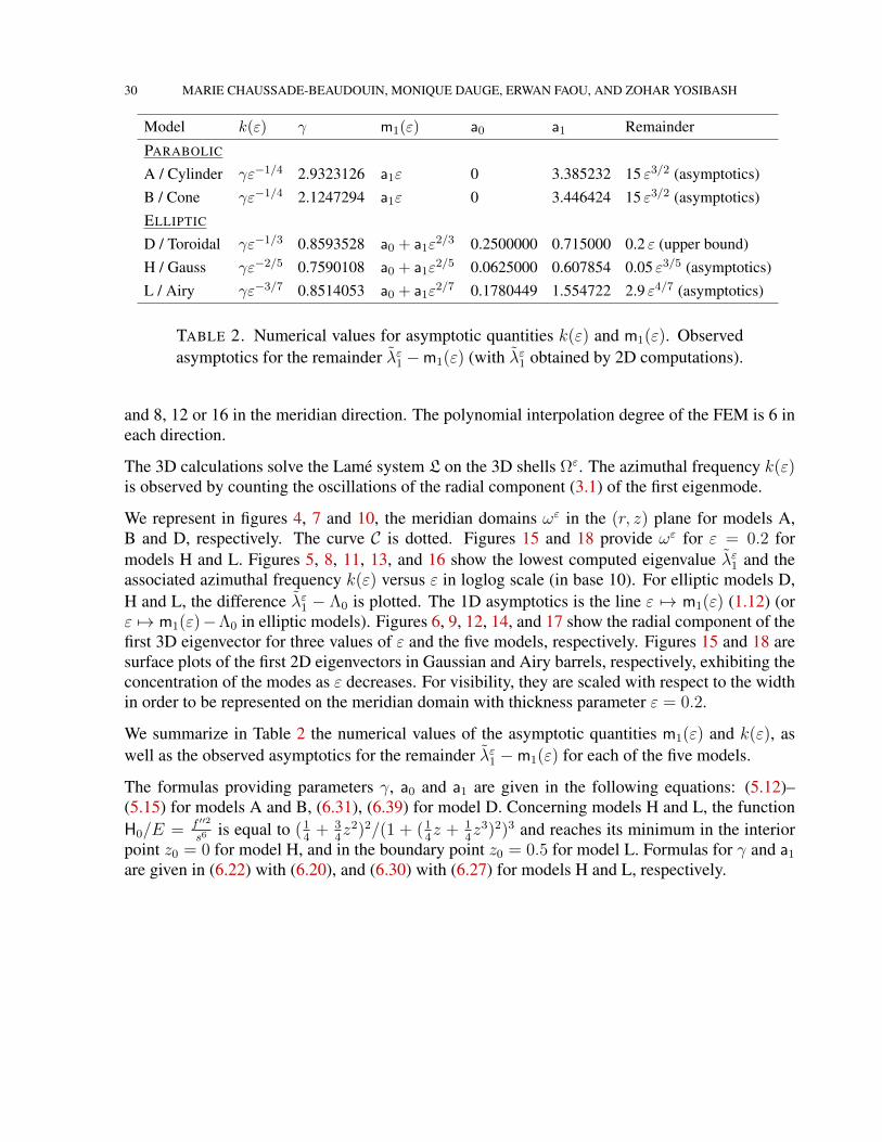
Model k(ε) γ m1(ε) a0 a1 Remainder
PARABOLIC
A / Cylinder γε−1/4 2.9323126 a1ε 0 3.385232 15 ε3/2 (asymptotics)B / Cone γε−1/4 2.1247294 a1ε 0 3.446424 15 ε3/2 (asymptotics)ELLIPTIC
D / Toroidal γε−1/3 0.8593528 a0 + a1ε2/3 0.2500000 0.715000 0.2 ε (upper bound)
H / Gauss γε−2/5 0.7590108 a0 + a1ε2/5 0.0625000 0.607854 0.05 ε3/5 (asymptotics)
L / Airy γε−3/7 0.8514053 a0 + a1ε2/7 0.1780449 1.554722 2.9 ε4/7 (asymptotics)
TABLE 2. Numerical values for asymptotic quantities k(ε) and m1(ε). Observedasymptotics for the remainder λε1 −m1(ε) (with λε1 obtained by 2D computations).
and 8, 12 or 16 in the meridian direction. The polynomial interpolation degree of the FEM is 6 ineach direction.
The 3D calculations solve the Lame system L on the 3D shells Ωε. The azimuthal frequency k(ε)is observed by counting the oscillations of the radial component (3.1) of the first eigenmode.
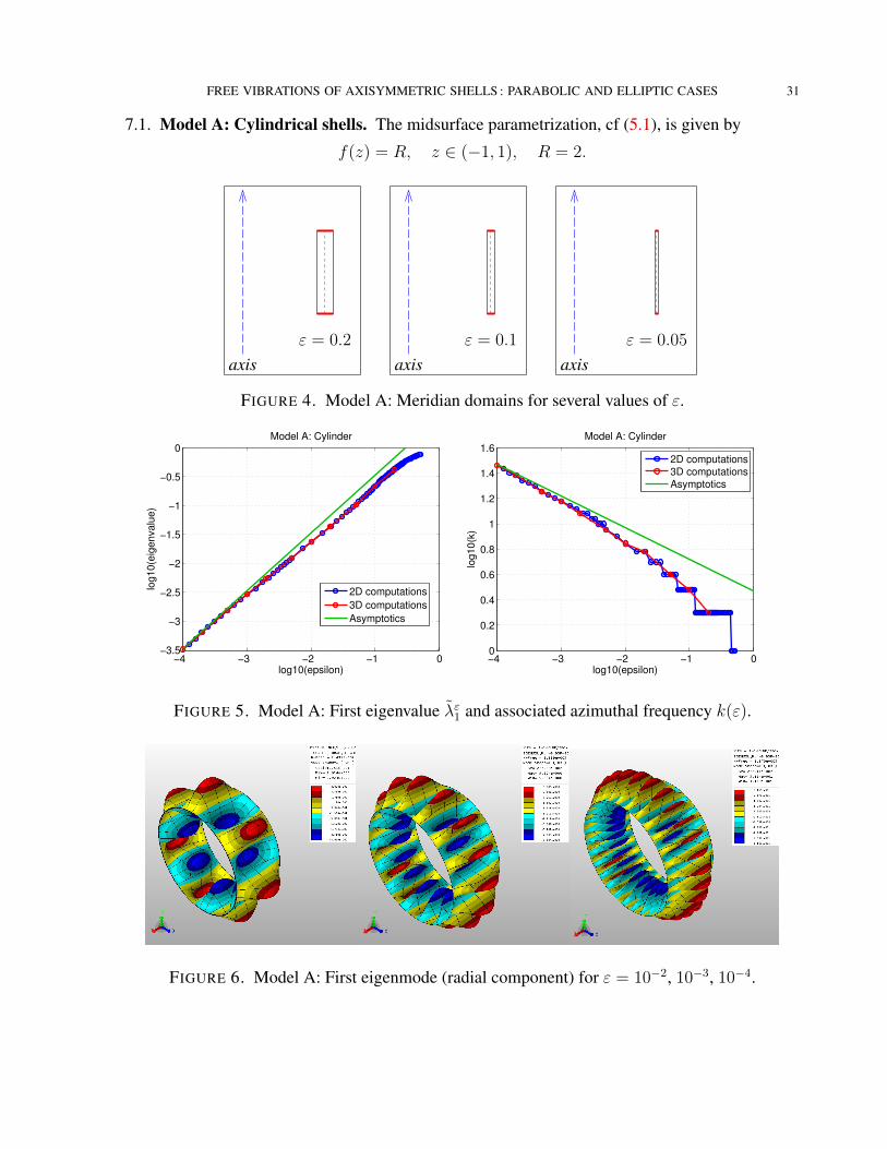
We represent in figures 4, 7 and 10, the meridian domains ωε in the (r, z) plane for models A,B and D, respectively. The curve C is dotted. Figures 15 and 18 provide ωε for ε = 0.2 formodels H and L. Figures 5, 8, 11, 13, and 16 show the lowest computed eigenvalue λε1 and theassociated azimuthal frequency k(ε) versus ε in loglog scale (in base 10). For elliptic models D,H and L, the difference λε1 − Λ0 is plotted. The 1D asymptotics is the line ε 7→ m1(ε) (1.12) (orε 7→ m1(ε)−Λ0 in elliptic models). Figures 6, 9, 12, 14, and 17 show the radial component of thefirst 3D eigenvector for three values of ε and the five models, respectively. Figures 15 and 18 aresurface plots of the first 2D eigenvectors in Gaussian and Airy barrels, respectively, exhibiting theconcentration of the modes as ε decreases. For visibility, they are scaled with respect to the widthin order to be represented on the meridian domain with thickness parameter ε = 0.2.
We summarize in Table 2 the numerical values of the asymptotic quantities m1(ε) and k(ε), aswell as the observed asymptotics for the remainder λε1 −m1(ε) for each of the five models.
The formulas providing parameters γ, a0 and a1 are given in the following equations: (5.12)–(5.15) for models A and B, (6.31), (6.39) for model D. Concerning models H and L, the functionH0/E = f ′′2
s6is equal to (1
4+ 3
4z2)2/(1 + (1
4z + 1
4z3)2)3 and reaches its minimum in the interior
point z0 = 0 for model H, and in the boundary point z0 = 0.5 for model L. Formulas for γ and a1
are given in (6.22) with (6.20), and (6.30) with (6.27) for models H and L, respectively.
FREE VIBRATIONS OF AXISYMMETRIC SHELLS : PARABOLIC AND ELLIPTIC CASES 31
7.1. Model A: Cylindrical shells. The midsurface parametrization, cf (5.1), is given by
f(z) = R, z ∈ (−1, 1), R = 2.
axisε = 0.2
axisε = 0.1
axisε = 0.05
FIGURE 4. Model A: Meridian domains for several values of ε.
−4 −3 −2 −1 0−3.5
−3
−2.5
−2
−1.5
−1
−0.5
0
log10(epsilon)
log10(e
igenvalu
e)
Model A: Cylinder
2D computations
3D computations
Asymptotics
−4 −3 −2 −1 00
0.2
0.4
0.6
0.8
1
1.2
1.4
1.6
log10(epsilon)
log10(k
)
Model A: Cylinder
2D computations
3D computations
Asymptotics
FIGURE 5. Model A: First eigenvalue λε1 and associated azimuthal frequency k(ε).
FIGURE 6. Model A: First eigenmode (radial component) for ε = 10−2, 10−3, 10−4.
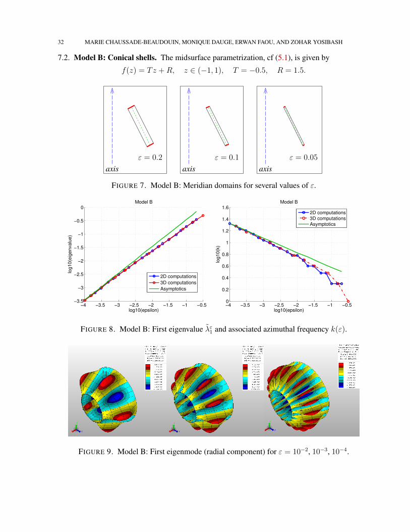
32 MARIE CHAUSSADE-BEAUDOUIN, MONIQUE DAUGE, ERWAN FAOU, AND ZOHAR YOSIBASH
7.2. Model B: Conical shells. The midsurface parametrization, cf (5.1), is given by
f(z) = Tz +R, z ∈ (−1, 1), T = −0.5, R = 1.5.
axisε = 0.2
axisε = 0.1
axisε = 0.05
FIGURE 7. Model B: Meridian domains for several values of ε.
−4 −3.5 −3 −2.5 −2 −1.5 −1 −0.5−3.5
−3
−2.5
−2
−1.5
−1
−0.5
0
log10(epsilon)
log10(e
igenvalu
e)
Model B
2D computations
3D computations
Asymptotics
−4 −3.5 −3 −2.5 −2 −1.5 −1 −0.50
0.2
0.4
0.6
0.8
1
1.2
1.4
1.6
log10(epsilon)
log10(k
)
Model B
2D computations
3D computations
Asymptotics
FIGURE 8. Model B: First eigenvalue λε1 and associated azimuthal frequency k(ε).
FIGURE 9. Model B: First eigenmode (radial component) for ε = 10−2, 10−3, 10−4.
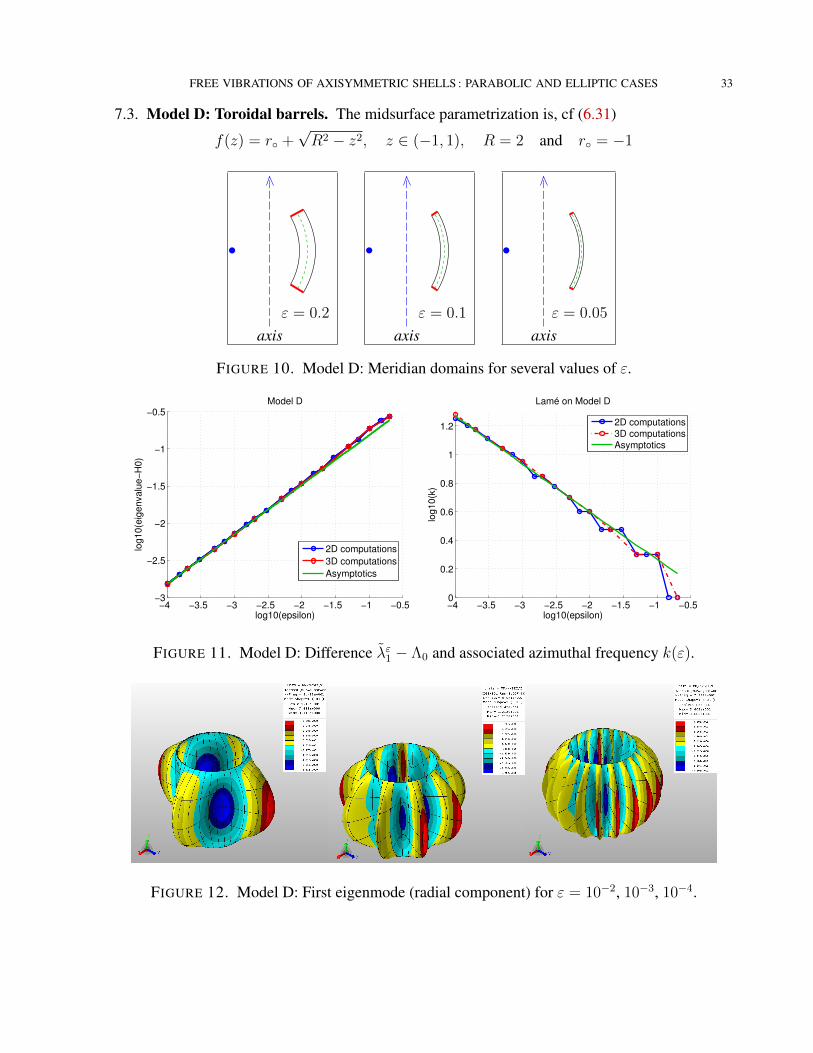
FREE VIBRATIONS OF AXISYMMETRIC SHELLS : PARABOLIC AND ELLIPTIC CASES 33
7.3. Model D: Toroidal barrels. The midsurface parametrization is, cf (6.31)
f(z) = r +√R2 − z2, z ∈ (−1, 1), R = 2 and r = −1
axisε = 0.2
•
axisε = 0.1
•
axisε = 0.05
•
FIGURE 10. Model D: Meridian domains for several values of ε.
−4 −3.5 −3 −2.5 −2 −1.5 −1 −0.5−3
−2.5
−2
−1.5
−1
−0.5
log10(epsilon)
log10(e
igenvalu
e−
H0)
Model D
2D computations
3D computations
Asymptotics
−4 −3.5 −3 −2.5 −2 −1.5 −1 −0.50
0.2
0.4
0.6
0.8
1
1.2
log10(epsilon)
log10(k
)
Lamé on Model D
2D computations
3D computations
Asymptotics
FIGURE 11. Model D: Difference λε1 − Λ0 and associated azimuthal frequency k(ε).
FIGURE 12. Model D: First eigenmode (radial component) for ε = 10−2, 10−3, 10−4.
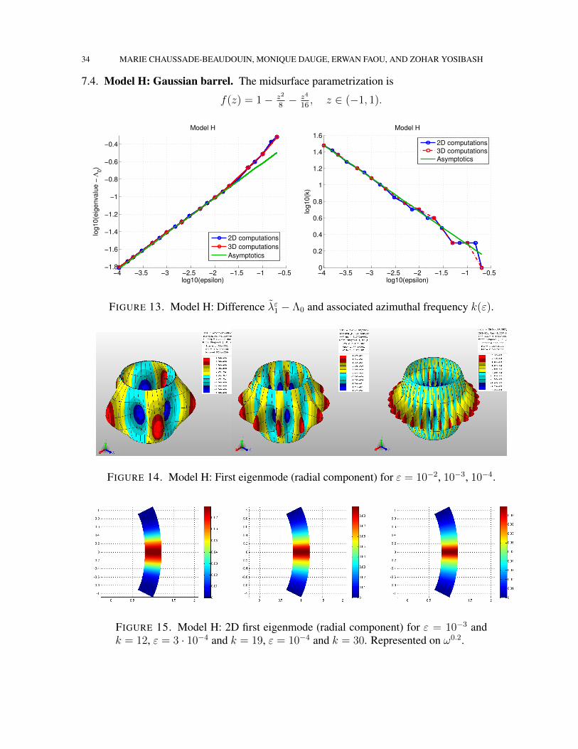
34 MARIE CHAUSSADE-BEAUDOUIN, MONIQUE DAUGE, ERWAN FAOU, AND ZOHAR YOSIBASH
7.4. Model H: Gaussian barrel. The midsurface parametrization is
f(z) = 1− z2
8− z4
16, z ∈ (−1, 1).
−4 −3.5 −3 −2.5 −2 −1.5 −1 −0.5−1.8
−1.6
−1.4
−1.2
−1
−0.8
−0.6
−0.4
log10(epsilon)
log10(e
igenvalu
e −
Λ0)
Model H
2D computations
3D computations
Asymptotics
−4 −3.5 −3 −2.5 −2 −1.5 −1 −0.50
0.2
0.4
0.6
0.8
1
1.2
1.4
1.6
log10(epsilon)
log10(k
)
Model H
2D computations
3D computations
Asymptotics
FIGURE 13. Model H: Difference λε1 − Λ0 and associated azimuthal frequency k(ε).
FIGURE 14. Model H: First eigenmode (radial component) for ε = 10−2, 10−3, 10−4.
FIGURE 15. Model H: 2D first eigenmode (radial component) for ε = 10−3 andk = 12, ε = 3 · 10−4 and k = 19, ε = 10−4 and k = 30. Represented on ω0.2.
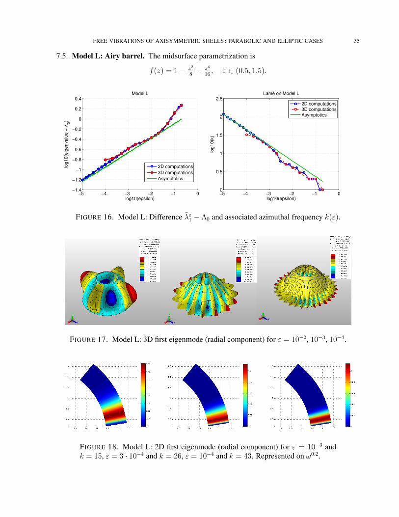
FREE VIBRATIONS OF AXISYMMETRIC SHELLS : PARABOLIC AND ELLIPTIC CASES 35
7.5. Model L: Airy barrel. The midsurface parametrization is
f(z) = 1− z2
8− z4
16, z ∈ (0.5, 1.5).
−5 −4 −3 −2 −1 0−1.4
−1.2
−1
−0.8
−0.6
−0.4
−0.2
0
0.2
0.4
log10(epsilon)
log10(e
igenvalu
e −
Λ0)
Model L
2D computations
3D computations
Asymptotics
−5 −4 −3 −2 −1 00
0.5
1
1.5
2
2.5
log10(epsilon)
log10(k
)
Lamé on Model L
2D computations
3D computations
Asymptotics
FIGURE 16. Model L: Difference λε1 − Λ0 and associated azimuthal frequency k(ε).
FIGURE 17. Model L: 3D first eigenmode (radial component) for ε = 10−2, 10−3, 10−4.
FIGURE 18. Model L: 2D first eigenmode (radial component) for ε = 10−3 andk = 15, ε = 3 · 10−4 and k = 26, ε = 10−4 and k = 43. Represented on ω0.2.

36 MARIE CHAUSSADE-BEAUDOUIN, MONIQUE DAUGE, ERWAN FAOU, AND ZOHAR YOSIBASH
8. CONCLUSION
For five categories of clamped axisymmetric shells, we have exhibited a scalar 1D operator thatdetermines the asymptotic expansion of the azimuthal frequency k(ε) of the first vibration mode,and a two-term asymptotic expansion for m1(ε) = a0 + a1ε
α1 for the first eigenvalue of the full3D Lame system in the shell. These five categories are the cylinders and the trimmed cones (par-abolic shells), as well as what we denote toroidal, Gaussian and Airy barrels (elliptic shells). Themost striking outcome of our analysis is the extremely good agreement of the three computationmethods (3D, 2D and 1D) in all the five cases described above, strengthening the relevance of ourconstructions. The presented methods demonstrate that the smallest eigenpairs for the Lame sys-tem can be estimated for specific shells by the reduced 1D model. Furthermore, the spreading orthe concentration of the first eigenmode can be predicted accurately: The cases for which concen-tration occurs are the Gauss and Airy barrels and for those shells, the first eigenmode concentratesaround a ring whose location (f(z0), z0) is analytically known.
Another interesting observation is the comparison with the computations in [3]. The elliptic casethat is considered there is f(z) = 1 − 1
2z2 on the interval I = (−a, a) with a = 0.892668. For
this example we find
g(z) = 32z2(1− 1
2z2) and H0(z) = (1 + z2)−3.
So we see that we are in our admissible ‘Airy’ case, predicting a behavior in ε−3/7 for the azimuthalfrequency k(ε) of the first eigenvector. Noting that 3
7' 0.43 and 2
5= 0.4, we believe that this
explains what have observed the authors [3, p.55]: “We also notice that in the elliptic case, Kt
[k(ε)] is probably growing slightly faster than exactly t−2/5 [ε−2/5]”.
APPENDIX A. HIGH FREQUENCY REDUCTION OF THE MEMBRANE OPERATOR
Recall that the membrane operator is written as M[k] = k2M0 + kM1 +M2. Let us give elementsof the proof of Theorem 4.2. We write the reduction formula (4.6) in the form
M[k]V[k] = V0 (H[k]− Λ[k]) + Λ[k]AV[k] .
This formula holds in the sense of the formal series algebra: This means that it is equivalent to thecollection of equations: For all n ≥ 0,
M0Vn + M1Vn−1 + M2Vn−2 = V0 (Hn−2 − Λn−2) +∑
p+q=n−2
ΛpAVq. (A.1)
with the convention that Vn, Hn, and Λn are 0 for n < 0, where Vn and Hn are the unknowncoefficients of the formal series V[k] =
∑n≥0 h
nVn and H[k] =∑
n≥0 hnHn. Here the series
Λ[k] =∑
n≥0 hnΛn is given. The mass matrix A is given by (4.2), and the operators M` by
M0 =E
1− ν2
1−ν
2f2s20 0
0 1f4
0
0 0 0
=:
Mzz0 0 0
0 Mϕϕ0 0
0 0 0
. (A.2)
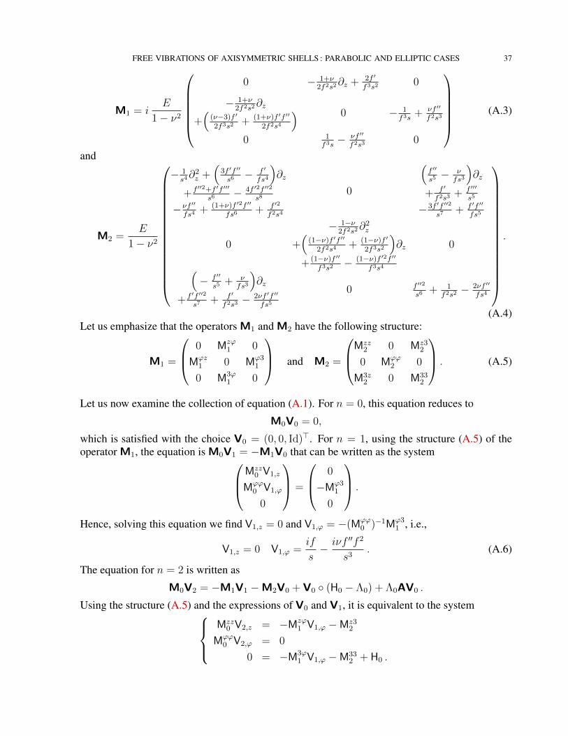
FREE VIBRATIONS OF AXISYMMETRIC SHELLS : PARABOLIC AND ELLIPTIC CASES 37
M1 = iE
1− ν2
0 − 1+ν
2f2s2∂z + 2f ′
f3s20
− 1+ν2f2s2
∂z
+(
(ν−3)f ′
2f3s2+ (1+ν)f ′f ′′
2f2s4
) 0 − 1f3s
+ νf ′′
f2s3
0 1f3s− νf ′′
f2s30
(A.3)
and
M2 =E
1− ν2
− 1s4∂2z +
(3f ′f ′′
s6− f ′
fs4
)∂z
+f ′′2+f ′f ′′′
s6− 4f ′2f ′′2
s8
−νf ′′
fs4+ (1+ν)f ′2f ′′
fs6+ f ′2
f2s4
0
(f ′′
s5− ν
fs3
)∂z
+ f ′
f2s3+ f ′′′
s5
−3f ′f ′′2
s7+ f ′f ′′
fs5
0
− 1−ν2f2s2
∂2z
+(
(1−ν)f ′f ′′
2f2s4+ (1−ν)f ′
2f3s2
)∂z
+ (1−ν)f ′′
f3s2− (1−ν)f ′2f ′′
f3s4
0
(− f ′′
s5+ ν
fs3
)∂z
+f ′f ′′2
s7+ f ′
f2s3− 2νf ′f ′′
fs5
0 f ′′2
s6+ 1
f2s2− 2νf ′′
fs4
.
(A.4)Let us emphasize that the operators M1 and M2 have the following structure:
M1 =
0 Mzϕ1 0
Mϕz1 0 Mϕ3
1
0 M3ϕ1 0
and M2 =
Mzz2 0 Mz3
2
0 Mϕϕ2 0
M3z2 0 M33
2
. (A.5)
Let us now examine the collection of equation (A.1). For n = 0, this equation reduces to
M0V0 = 0,
which is satisfied with the choice V0 = (0, 0, Id)>. For n = 1, using the structure (A.5) of theoperator M1, the equation is M0V1 = −M1V0 that can be written as the systemMzz
0 V1,z
Mϕϕ0 V1,ϕ
0
=
0
−Mϕ31
0
.
Hence, solving this equation we find V1,z = 0 and V1,ϕ = −(Mϕϕ0 )−1Mϕ3
1 , i.e.,
V1,z = 0 V1,ϕ =if
s− iνf ′′f 2
s3. (A.6)
The equation for n = 2 is written as
M0V2 = −M1V1 −M2V0 + V0 (H0 − Λ0) + Λ0AV0 .
Using the structure (A.5) and the expressions of V0 and V1, it is equivalent to the systemMzz
0 V2,z = −Mzϕ1 V1,ϕ −Mz3
2
Mϕϕ0 V2,ϕ = 0
0 = −M3ϕ1 V1,ϕ −M33
2 + H0 .
38 MARIE CHAUSSADE-BEAUDOUIN, MONIQUE DAUGE, ERWAN FAOU, AND ZOHAR YOSIBASH
The last equation of the previous system joint with (A.6) gives the expression of the operator H0
H0 = M332 −M3ϕ
1 (Mϕϕ0 )−1Mϕ3
1 ,
and using the first two equations, we can solve for V2 by setting
V2,z = (Mzz0 )−1(Mzϕ
1 (Mϕϕ0 )−1Mϕ3
1 −Mz32 ) and V2,ϕ = (Mϕϕ
0 )−1aϕϕΛ0.
Thus we find that H0 = E f ′′2
s6and that the components of V2 are
V2,ϕ = 0,
V2,z =(− f
s− (ν + 2)f 2f ′′
s3
)∂z
+f ′
s+
3(ν + 2)f 2f ′f ′′2
s5− (ν + 2)f 2f ′′′
s3− (2ν + 1)ff ′f ′′
s3. (A.7)
Now let us assume that the operators Ln and Vn+1 are constructed for n ≥ 1. Then writing theequation (A.1) for n+ 2, we obtain the relation (using the fact that −V0Λn + ΛnAV0 = 0)
M0Vn+2 − V0 Hn = −M1Vn+1 −M2Vn +n−1∑p=0
ΛpAVn−p .
This equation is equivalent to the system (using the fact that Vn,3 = 0 for n ≥ 1)Mρρ
0 Vn+2,z = −Mzϕ1 Vn+1,ϕ −Mzz
2 Vn,z +∑n−1
p=0 ΛpazzVn−p,z
Mϕϕ0 Vn+2,ϕ = −Mϕz
1 Vn+1,z −Mϕϕ2 Vn,ϕ +
∑n−1p=0 Λpa
ϕϕVn−p,ϕ
Hn = M3ϕ1 Vn+1,ϕ + M3z
2 Vn,z ,
which gives the existence of the operators Vn+2,z, Vn+2,ϕ and Hn. This shows the existence of theoperators Vn = (Vn,z,Vn,ϕ, 0)>. Moreover, we can check that Vn is an operator of order n − 1and is polynomial in Λj , for j ≤ n− 3. The scalar operators Hn are of order n, polynomial in Λj ,for j ≤ n− 2.
Expressions of the operators Hn for n = 0, . . . , 4 are given by the formulas (6.1)–(6.4) and thecomponents of the operator V3 are given by
V3,z = 0,
V3,ϕ = i(− νf 3
s3− (1 + 2ν)f 4f ′′
s5
)∂2z
+ i(− (4ν + 6)f 3f ′f ′′
s5− (4ν + 2)f 4f ′′′
s5+
7(2ν + 1)f 4f ′f ′′2
s7− f 2f ′
s3
)∂z
+ i((ν2 + 19ν + 19)f 3f ′2f ′′2
s7− (6ν + 6)f 3f ′f ′′′
s5− (5ν + 3)f 2f ′2f ′′
s5
− (36ν + 18)f 4f ′2f ′′3
s9+
(20ν + 10)f 4f ′f ′′f ′′′
s7+νf ′′f 2
s3+f ′2f
s3
+(6ν + 3)f 4f ′′3
s7− (2ν + 1)f 4f (4)
s5− (ν2 + ν + 1)f 3f ′′2
s5
)+ i
1− ν2
EΛ0
(f 3
s− νf 4f ′′
s3
). (A.8)
FREE VIBRATIONS OF AXISYMMETRIC SHELLS : PARABOLIC AND ELLIPTIC CASES 39
APPENDIX B. VARIATIONAL FORMULATIONS ON THE MERIDIAN DOMAIN
The 3D Lame operator is independent of the azimuthal coordinate ϕ if expressed in cylindricalcomponents of displacements. The contravariant cylindrical components used in this paper are
ur = ut1 cosϕ+ ut2 sinϕ, (radial)uϕ = −ut1 1
rsinϕ+ ut2 1
rcosϕ, (azimuthal)
uτ = ut3 (axial).
For a displacement u defined on Ωε, denote by uk = (urk, uϕk , u
τk) the Fourier coefficients of these
components:
uak(r, τ) =1
2π
∫ 2π
0
ua(r, ϕ, τ) e−ikϕ dϕ, a ∈ r, ϕ, τ, k ∈ Z, (r, τ) ∈ ωε.
The energy bilinear form aε3D is decomposed in Fourier coefficients as follows
aε3D(u, v) =∑k∈Z
aεk(uk, vk) .
As soon as k 6= 0, the energy bilinear form aεk at azimuthal frequency k as non real coefficients.Nevertheless, by a simple change of components, the coefficients are back to real:
aεk((ur, iuϕ, uτ ), (vr,− ivϕ, vτ )
)=
E
1− ν2
∫ωε
(1− ν)2
1− 2ν
(r∂ru
r∂rvr + r∂τu
τ∂τvτ +
k2
r3uϕvϕ +
1
rurvr
)+ν(1− ν)
1− 2νr(∂ru
r∂τvτ + ∂τu
τ∂rvr)
+ν(1− ν)
1− 2ν
(∂ru
rvr + ur∂rvr + ur∂τv
τ + ∂τuτvr)
+1− ν
2
k2
r
(urvr + uτvτ
)+
1− ν2
1
r
(∂ru
ϕ∂rvϕ − 2
r∂ru
ϕvϕ − 2
ruϕ∂rv
ϕ +4
r2uϕvϕ + ∂τu
ϕ∂τvϕ)
+1− ν
2r(∂ru
τ∂τvr + ∂τu
r∂rvτ + ∂ru
τ∂rvτ + ∂τu
r∂τvr)
+ k
[(1− ν)2
1− 2ν
1
r2
(uϕvr + urvϕ
)+
1− νr2
(uϕvr + urvϕ
)+ν(1− ν)
1− 2ν
1
r
(uϕ∂rv
r + ∂rurvϕ + uϕ∂τv
τ + ∂τuτvϕ)
− 1− ν2
1
r
(uτ∂τv
ϕ + ∂τuϕvτ + ur∂rv
ϕ + ∂ruϕvr)]
drdτ
The associate eigenproblem is: Find λ and a nonzero (ur, uϕ, uτ ) ∈ V (ωε) such that for all(vr, vϕ, vτ ) ∈ V (ωε)
aεk((ur, iuϕ, uτ ), (vr,−ivϕ, vτ )
)= λ
∫ωε
[urvr +1
r2uϕvϕ + uτvτ ] rdrdτ.
40 MARIE CHAUSSADE-BEAUDOUIN, MONIQUE DAUGE, ERWAN FAOU, AND ZOHAR YOSIBASH
Here the variational space V (ωε) corresponds to V (Ωε)
V (ωε) := u = (ur, uϕ, uτ ) ∈ H1(ωε)3 , u = 0 on ∂0ωε.
Note that the eigenvalues of aεk are the same as those of aε−k because of the identity
aε−k((ur, iuϕ, uτ ), (vr,−ivϕ, vτ )
)= aεk
((ur,−iuϕ, uτ ), (vr, ivϕ, vτ )
).
REFERENCES
[1] S. AGMON, A. DOUGLIS, AND L. NIRENBERG, Estimates near the boundary for solutions of elliptic partialdifferential equations satisfying general boundary conditions II, Comm. Pure Appl. Math., 17 (1964), pp. 35–92.
[2] E. ARTIOLI, L. BEIRAO DA VEIGA, H. HAKULA, AND C. LOVADINA, Free vibrations for some Koiter shellsof revolution., Appl. Math. Lett., 12 (2008 (21)), pp. 1245–1248.
[3] , On the asymptotic behaviour of shells of revolution in free vibration., Computational Mechanics, 44(2009), pp. 45–60.
[4] F. ATKINSON, H. LANGER, R. MENNICKEN, AND A. A. SHKALIKOV, The essential spectrum of some matrixoperators., Math. Nach., 167 (1994), pp. 5–20.
[5] M. BEAUDOUIN, Modal analysis for thin axisymmetric shells, theses, Universite Rennes 1, Nov. 2010,https://tel.archives-ouvertes.fr/tel-00541467.
[6] L. BEIRAO DA VEIGA, H. HAKULA, AND J. PITKARANTA, Asymptotic and numerical analysis of the eigen-value problem for a clamped cylindrical shell., Math. Models Methods Appl. Sci., 18 (11) (2008), pp. 1983–2002.
[7] L. BEIRAO DA VEIGA AND C. LOVADINA, An interpolation theory approach to shell eigenvalue problems.,Math. Models Methods Appl. Sci., 18 (12) (2008), pp. 2003–2018.
[8] M. BERNADOU AND P. G. CIARLET, Sur l’ellipticite du modele lineaire de coques de W.T.Koiter., in Comput-ing Methods in Applied Sciences and Engineering, R.Glowinski and J.L.Lions, eds., Lecture Notes in Econom-ics and Mathematical Systems, Vol.134, Springer-Verlag, Heidelberg, 1976, pp. 89–136.
[9] P. G. CIARLET, Mathematical elasticity. Vol. III, North-Holland Publishing Co., Amsterdam, 2000. Theory ofshells.
[10] P. G. CIARLET AND S. KESAVAN, Two-dimensional approximation of three-dimensional eigenvalue problemsin plate theory, Comp. Methods Appl. Mech. Engrg., 26 (1981), pp. 149–172.
[11] P. G. CIARLET AND V. LODS, Asymptotic analysis of linearly elastic shells. I. Justification of membrane shellequations, Arch. Rational Mech. Anal., 136 (1996), pp. 119–161.
[12] , Asymptotic analysis of linearly elastic shells. III. Justification of Koiter’s shell equations, Arch. RationalMech. Anal., 136 (1996), pp. 191–200.
[13] P. G. CIARLET, V. LODS, AND B. MIARA, Asymptotic analysis of linearly elastic shells. II. Justification offlexural shell equations, Arch. Rational Mech. Anal., 136 (1996), pp. 163–190.
[14] M. DAUGE, I. DJURDJEVIC, E. FAOU, AND A. ROSSLE, Eigenmode asymptotics in thin elastic plates, J.Maths. Pures Appl., 78 (1999), pp. 925–964.
[15] M. DAUGE AND E. FAOU, Koiter estimate revisited, Math. Models Methods Appl. Sci., 20 (2010), pp. 1–42.[16] M. DAUGE, E. FAOU, AND Z. YOSIBASH, Plates and shells : Asymptotic expansions and hierarchical models,
Encyclopedia of Computational Mechanics, 1, chap 8 (2004), pp. 199–236.[17] M. DAUGE AND I. GRUAIS, Asymptotics of arbitrary order for a thin elastic clamped plate. II: Analysis of the
boundary layer terms, Asymptotic Analysis, 16 (1998), pp. 99–124.[18] M. P. DO CARMO, Differential geometry of curves and surfaces, Prentice Hall, 1976.[19] , Riemannian geometry, Mathematics : Theory and applications, Birkhauser, Boston, 1992.[20] E. FAOU, Elasticity on a thin shell: Formal series solution, Asymptotic Analysis, 31 (2002), pp. 317–361.[21] , Multiscale expansions for linear clamped elliptic shells, Comm. Partial Differential Equations, 29(11-12)
(2004), pp. 1799–1845.[22] K. GENEVEY, A regularity result for a linear membrane shell problem., RAIRO Model. Math. Anal. Numer.,
30 (4) (1996), pp. 467–488.[23] F. JOHN, Refined interior equations for thin elastic shells., Comm. Pure Appl. Math., 24 (1971), pp. 583–615.
FREE VIBRATIONS OF AXISYMMETRIC SHELLS : PARABOLIC AND ELLIPTIC CASES 41
[24] G. KIRCHHOFF, Uber das Gleichgewicht und die Bewegung einer elastischen Scheibe., Journ. Reine Angew.Math., 40 (1850), pp. 51–58.
[25] W. T. KOITER, A consistent first approximation in the general theory of thin elastic shells, Proc. IUTAM Sym-posium on the Theory on Thin Elastic Shells, August 1959, (1960), pp. 12–32.
[26] , On the foundations of the linear theory of thin elastic shells: I., Proc. Kon. Ned. Akad. Wetensch., Ser.B,73 (1970), pp. 169–182.
[27] , On the foundations of the linear theory of thin elastic shells: II., Proc. Kon. Ned. Akad. Wetensch., Ser.B,73 (1970), pp. 183–195.
[28] V. LODS AND C. MARDARE, Justification of linear Koiter and Naghdi’s models for totally clamped shell.,Asymptotic Anal., 31 (2002), pp. 189–210.
[29] D. MARTIN, Melina, bibliotheque de calculs elements finis.http://anum-maths.univ-rennes1.fr/melina/index.html (2008).
[30] R. D. MINDLIN, Influence of rotatory inertia and shear on flexural motions of isotropoic elastic plates, J. Appl.Mech., 18 (1951), pp. 31–38.
[31] P. M. NAGHDI, Foundations of elastic shell theory, in Progress in Solid Mechanics, vol. 4, North-Holland,Amsterdam, 1963, pp. 1–90.
[32] V. V. NOVOZHILOV, Thin Shell Theory, Walters-Noordhoff Publishing, Groningen, 1959.[33] J. PITKARANTA, A.-M. MATACHE, AND C. SCHWAB, Fourier mode analysis of layers in shallow shell defor-
mations, Comput. Methods Appl. Mech. Eng., 190 (2001), pp. 2943–2975.[34] E. REISSNER, On the theory of bending of elastic plates., J. Math. and Phys., 23 (1944), pp. 184–191.[35] J. SANCHEZ-HUBERT AND E. SANCHEZ-PALENCIA, Coques elastiques minces. Proprietes asymptotiques,
Recherches en mathematiques appliquees, Masson, Paris, 1997.[36] E. SANCHEZ-PALENCIA, Statique et dynamique des coques minces. I. Cas de flexion pure non inhibee., C. R.
Acad. Sci. Paris, Ser. I, 309 (1989), pp. 411–417.[37] , Statique et dynamique des coques minces. II. Cas de flexion pure inhibee. Approximation membranaire.,
C. R. Acad. Sci. Paris, Ser. I, 309 (1989), pp. 531–537.[38] , Passage a la limite de l’elasticite tridimensionnelle a la theorie asymptotique des coques minces, C. R.
Acad. Sci. Paris, Ser. II, 311 (1990), pp. 909–916.[39] M. SPIVAK, A comprehensive introduction to differential geometry, Publish or perish, 1979.
MC, MD & EF: IRMAR, (CNRS, INRIA) UNIVERSITE DE RENNES 1,CAMPUS DE BEAULIEU, 35042 RENNES CEDEX, FRANCE
ZY: BEN-GURION UNIVERSITY, DEPT. OF MECHANICAL ENGINEERING,POBOX 653, BEER-SHEVA 84105, ISRAEL
E-mail address: [email protected]
URL: http://perso.univ-rennes1.fr/monique.dauge/
E-mail address: [email protected]
URL: http://www.irisa.fr/ipso/perso/faou/
E-mail address: [email protected]
URL: http://www.bgu.ac.il/˜zohary/


![Physics design of a high- quasi-axisymmetric stellaratorphoenix.ps.uci.edu/zlin/bib/reiman99.pdf · axisymmetric (QA) [1,2]. This paper discusses key physics issues that have been](https://static.fdocument.org/doc/165x107/5f707848fb9ed6719236c307/physics-design-of-a-high-quasi-axisymmetric-axisymmetric-qa-12-this-paper.jpg)