Fourier, filtering, thi d ismoothing, and noise

Nuno Vasconcelos ECE Department, UCSDp ,

(with thanks to David Forsyth)

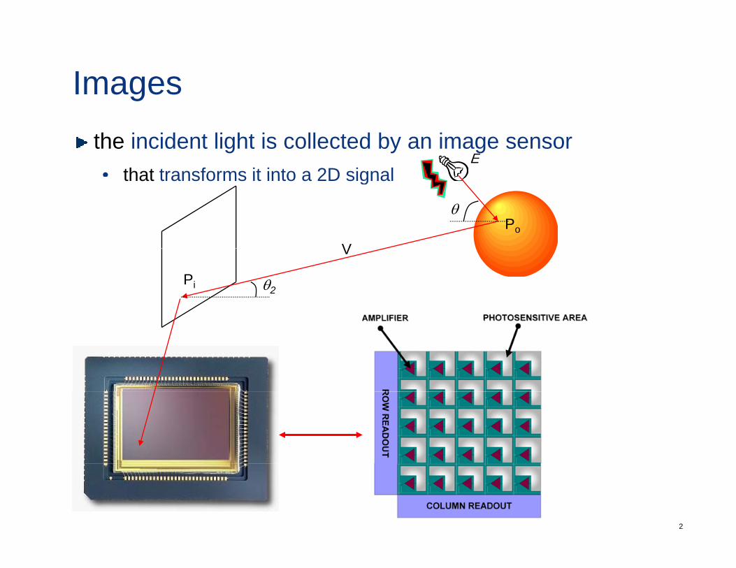
Imagesthe incident light is collected by an image sensor• that transforms it into a 2D signal

Ethat transforms it into a 2D signal

θPo

V

θ2Pi

V

2

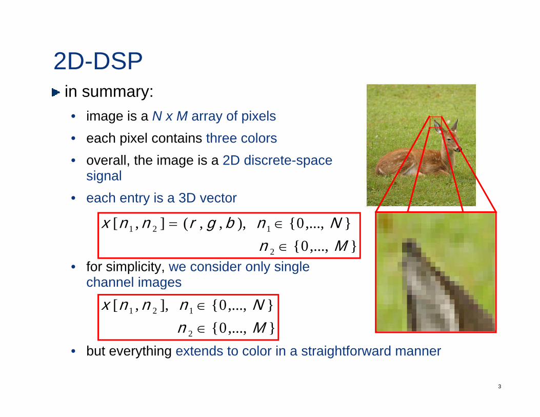
2D-DSPin summary:• image is a N x M array of pixels• each pixel contains three colors• overall, the image is a 2D discrete-space

signalg• each entry is a 3D vector

},...,0{),,,(],[ 121 Nnbgrnnx ∈=

• for simplicity, we consider only singlechannel images

},...,0{2 Mn ∈

g

},...,0{},...,0{],,[

2

121

MnNnnnx

∈∈

3

• but everything extends to color in a straightforward manner

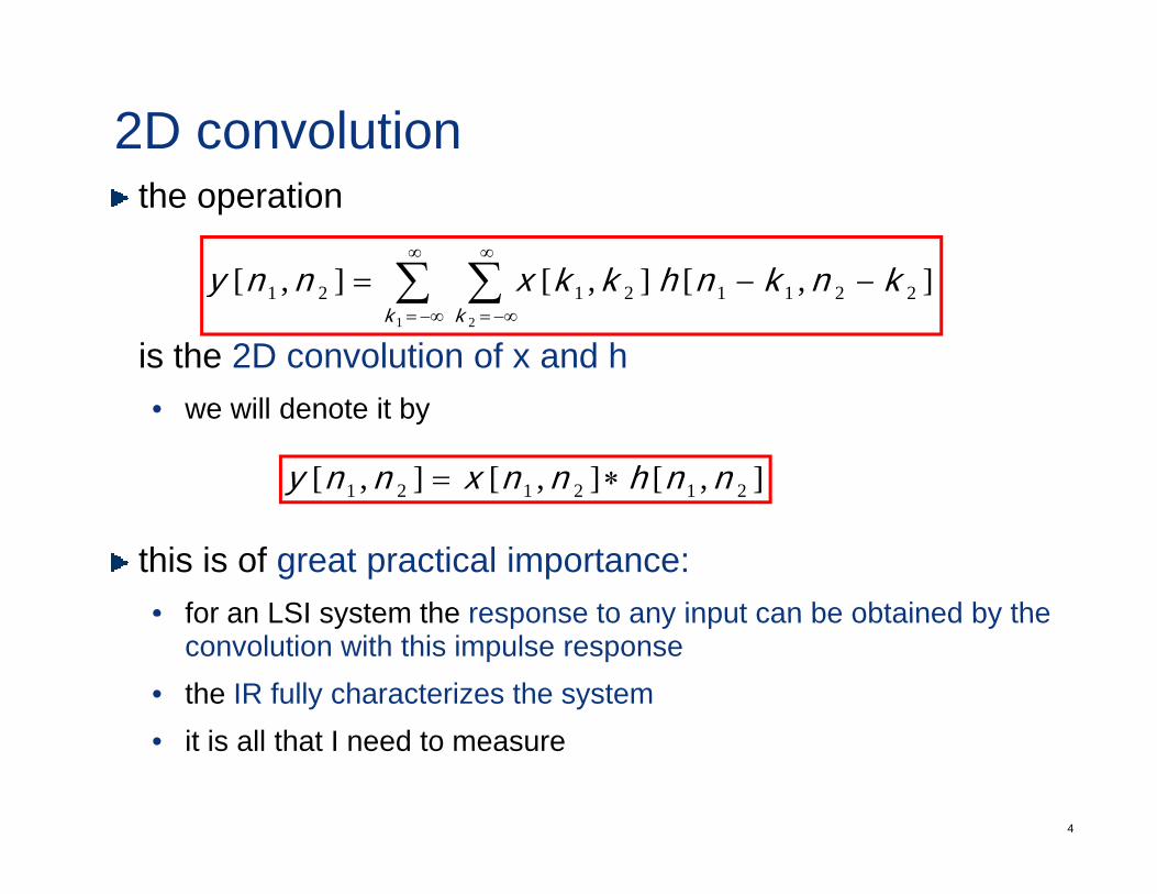
2D convolutionthe operation

][][][ knknhkkxnny ∑ ∑∞ ∞

is the 2D convolution of x and h

],[],[],[ 221121211 2

knknhkkxnnyk k

−−= ∑ ∑−∞= −∞=

• we will denote it by

],[],[],[ 212121 nnhnnxnny ∗=

this is of great practical importance:• for an LSI system the response to any input can be obtained by thefor an LSI system the response to any input can be obtained by the

convolution with this impulse response• the IR fully characterizes the system

4

• it is all that I need to measure

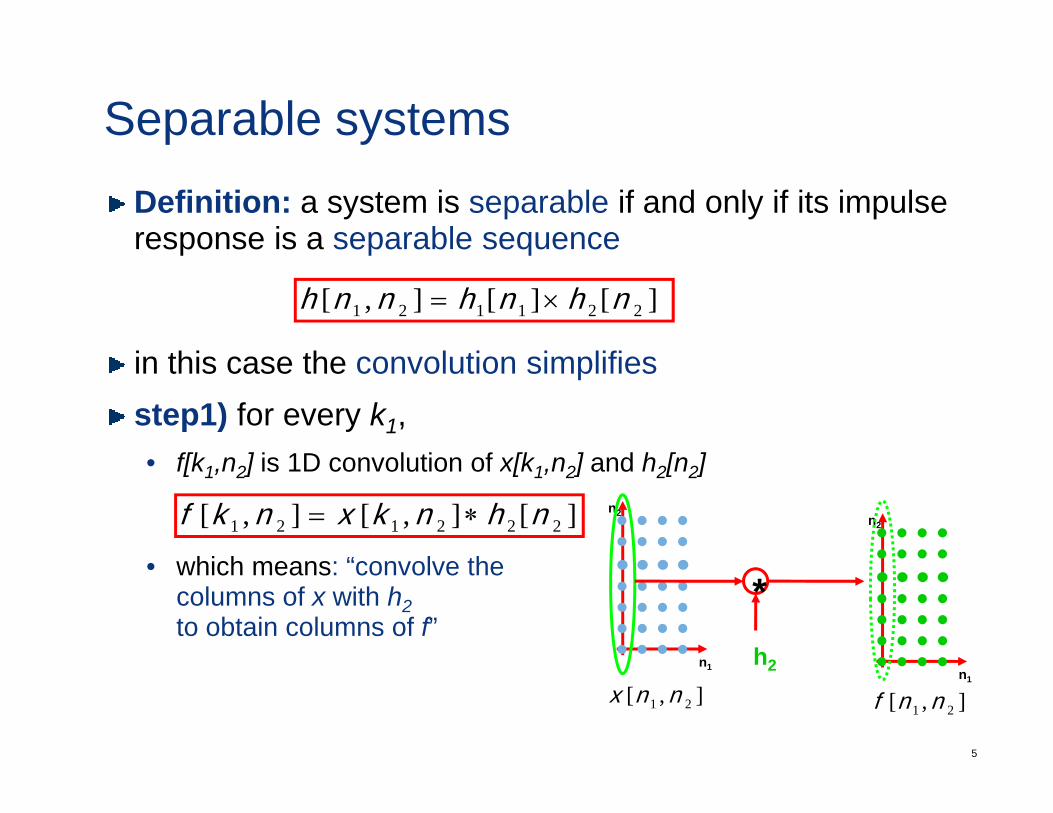
Separable systemsDefinition: a system is separable if and only if its impulse response is a separable sequencep p q

i thi th l ti i lifi

][][],[ 221121 nhnhnnh ×=

in this case the convolution simplifiesstep1) for every k1,

f[k n ] is 1D convolution of x[k n ] and h [n ]• f[k1,n2] is 1D convolution of x[k1,n2] and h2[n2]

hi h “ l th

][],[],[ 222121 nhnkxnkf ∗= n2 n2

• which means: “convolve the columns of x with h2to obtain columns of f”

n

*h2

5

n1 n1

h2

],[ 21 nnx ],[ 21 nnf

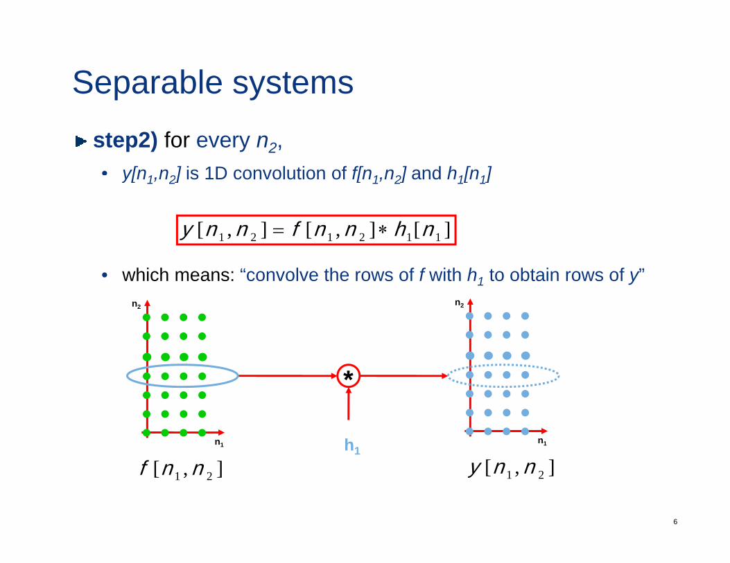
Separable systemsstep2) for every n2, • y[n1 n2] is 1D convolution of f[n1 n2] and h1[n1]y[n1,n2] is 1D convolution of f[n1,n2] and h1[n1]

][],[],[ 112121 nhnnfnny ∗=

• which means: “convolve the rows of f with h1 to obtain rows of y”n2n2

*

n1n1 h1

6

],[ 21 nny],[ 21 nnf

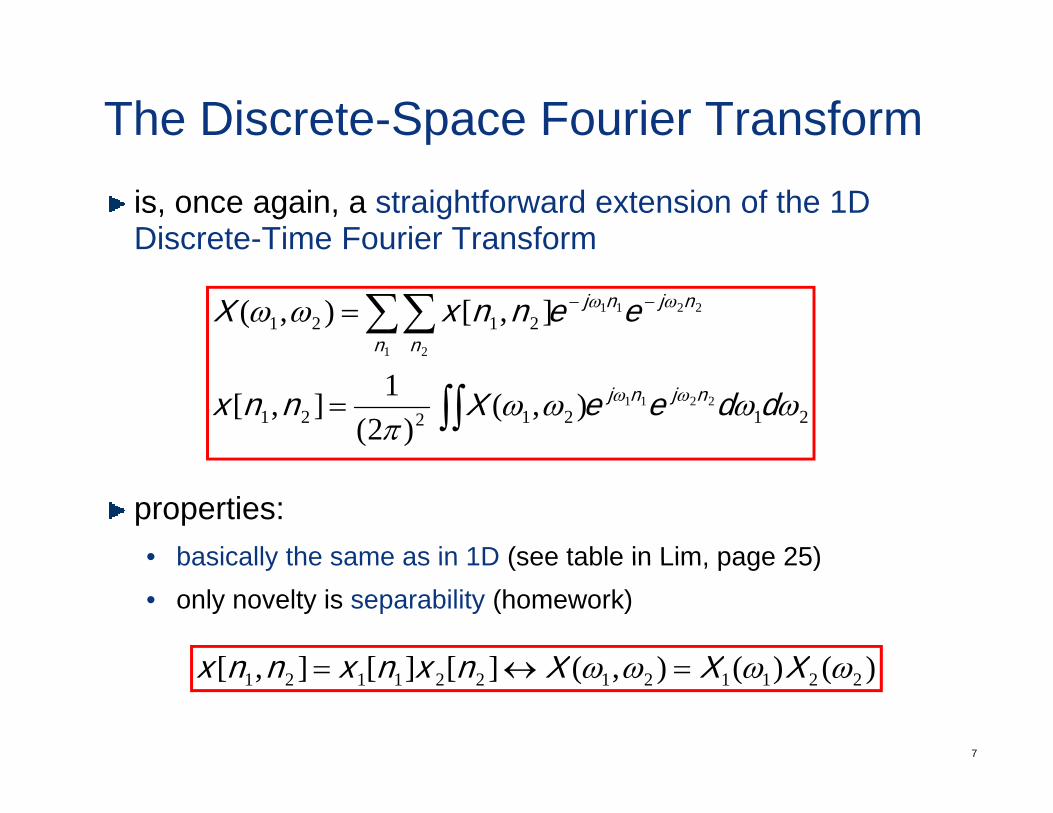
The Discrete-Space Fourier Transformis, once again, a straightforward extension of the 1D Discrete-Time Fourier Transform

21212211

1 2

],[),( ωω ωω eennxX njnj

n n∑∑= −−

21212212211

1 2

),()2(

1],[ ωωωωπ

ωω ddeeXnnx njnj∫∫=

properties:• basically the same as in 1D (see table in Lim page 25)basically the same as in 1D (see table in Lim, page 25)• only novelty is separability (homework)

)()()(][][][ XXXnxnxnnx ↔

7

)()(),(][][],[ 221121221121 ωωωω XXXnxnxnnx =↔=

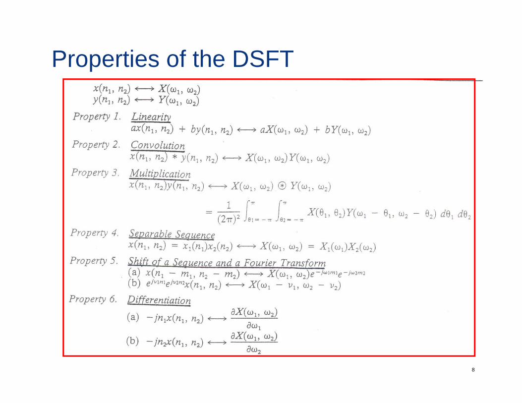
Properties of the DSFT

8

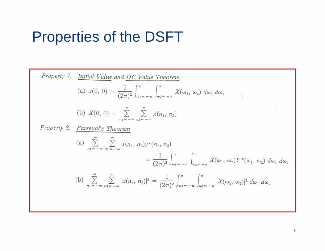
Properties of the DSFT

9

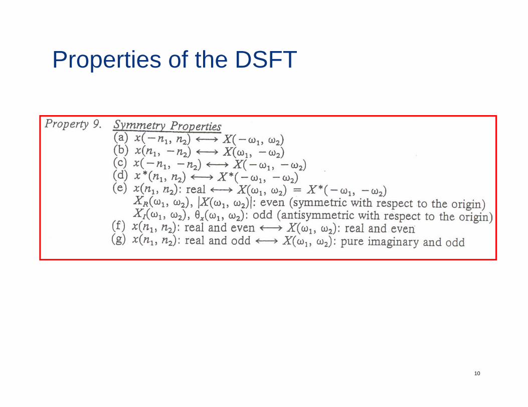
Properties of the DSFT

10

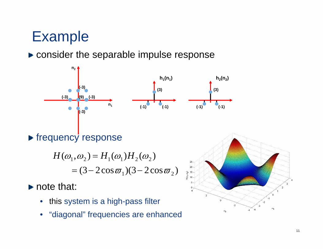
Exampleconsider the separable impulse response

n2

h (n ) h (n )

n1

(9) (-3)(-3)

(-3) (3)

(-1)(-1)

h1(n1)

(3)

(-1)(-1)

h2(n2)

frequency response

(-3)( )( ) ( )( )

frequency response

)cos23)(cos23( )()(),( 221121

ϖϖωωωω−−=

= HHH

note that: • this system is a high-pass filter

)cos23)(cos23( 21 ϖϖ=

11

this system is a high pass filter• “diagonal” frequencies are enhanced

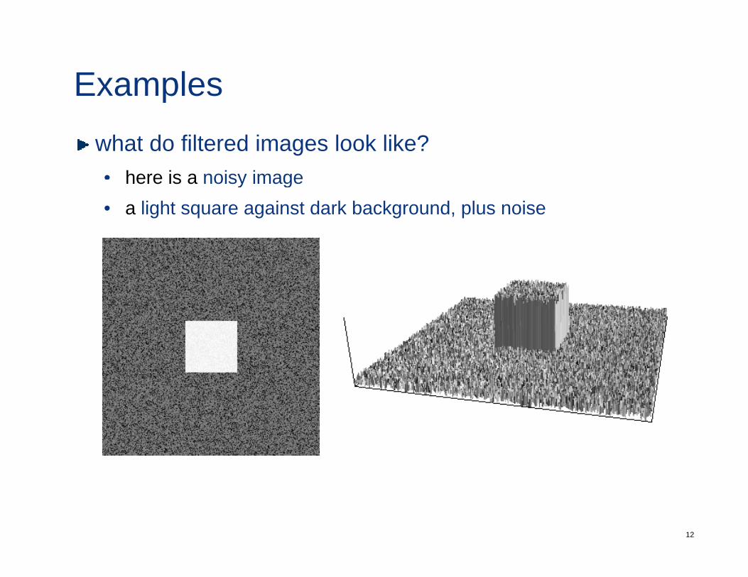
Exampleswhat do filtered images look like?• here is a noisy imagehere is a noisy image• a light square against dark background, plus noise

12

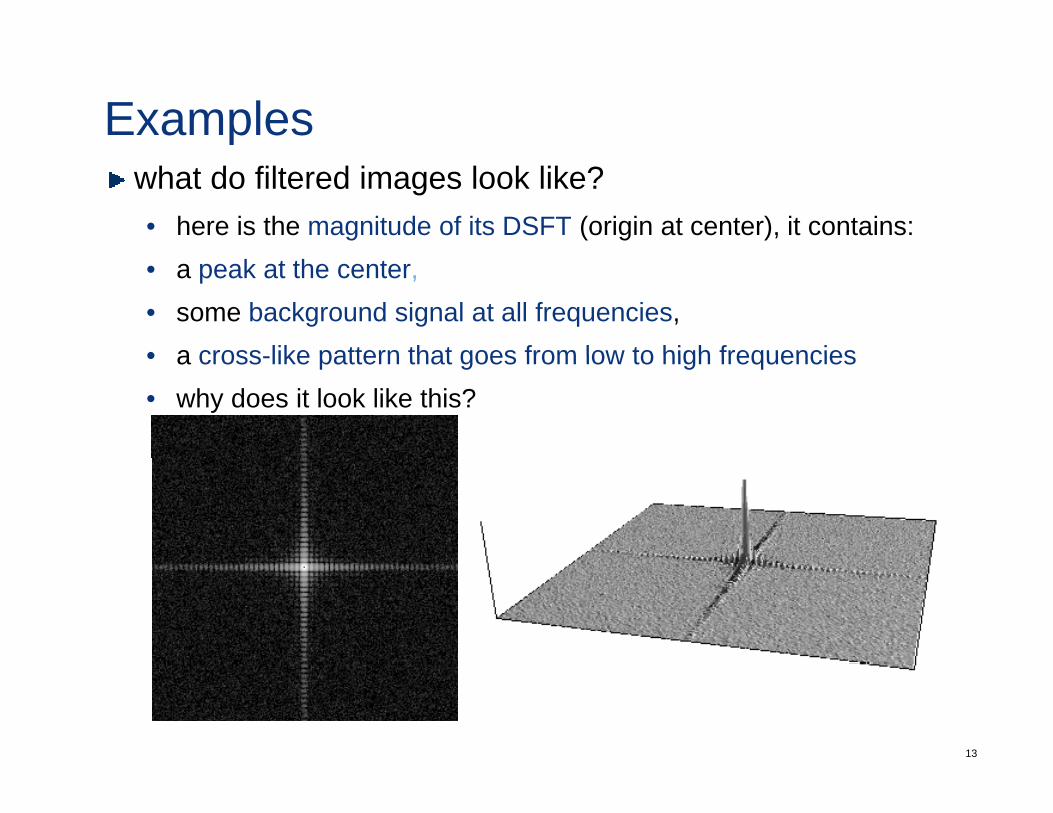
Exampleswhat do filtered images look like?• here is the magnitude of its DSFT (origin at center), it contains:• a peak at the center,• some background signal at all frequencies, • a cross like pattern that goes from low to high frequencies• a cross-like pattern that goes from low to high frequencies• why does it look like this?

13

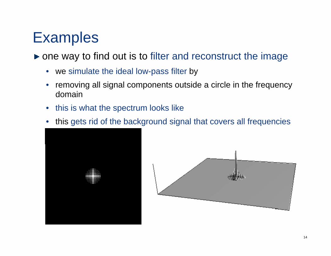
Examplesone way to find out is to filter and reconstruct the image• we simulate the ideal low-pass filter by • removing all signal components outside a circle in the frequency

domain• this is what the spectrum looks likep• this gets rid of the background signal that covers all frequencies

14

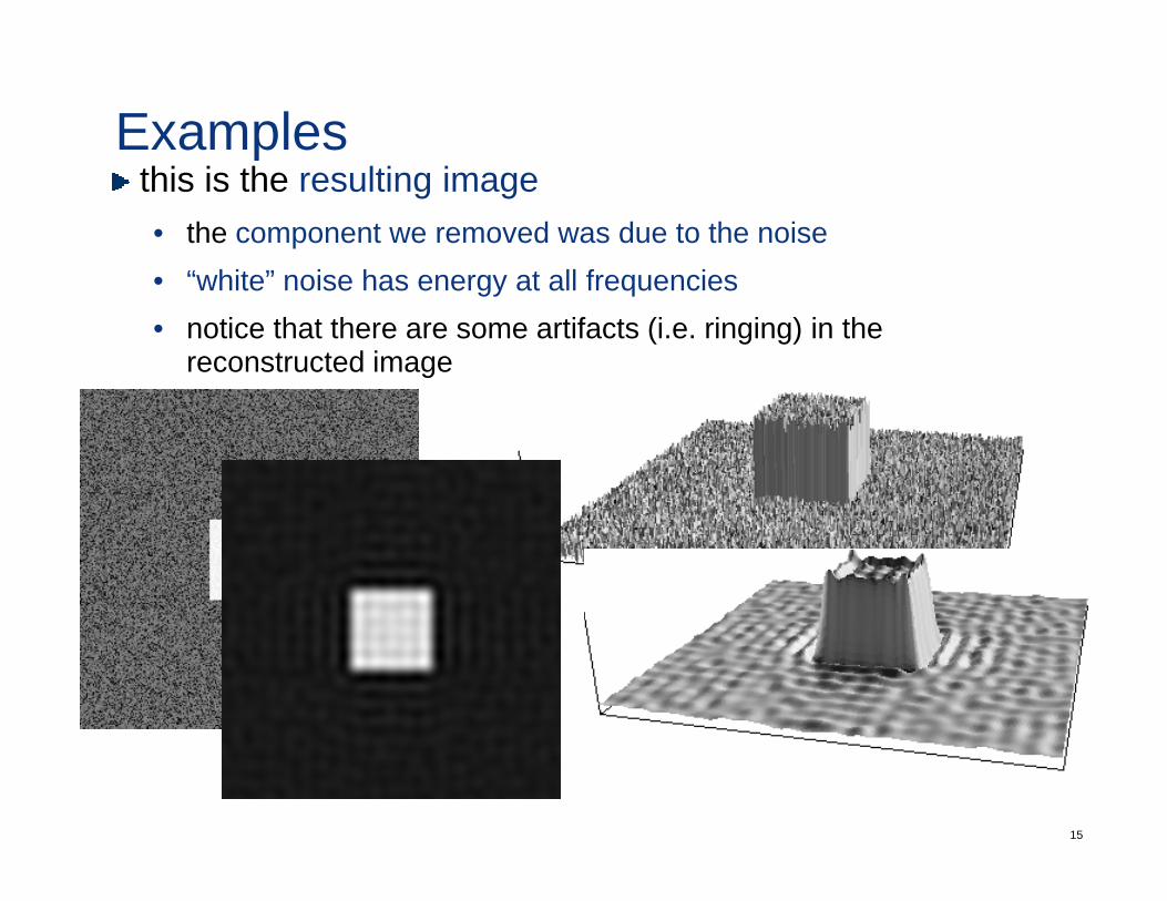
Exampleshi i h l i ithis is the resulting image• the component we removed was due to the noise• “white” noise has energy at all frequencies• white noise has energy at all frequencies• notice that there are some artifacts (i.e. ringing) in the

reconstructed image

15

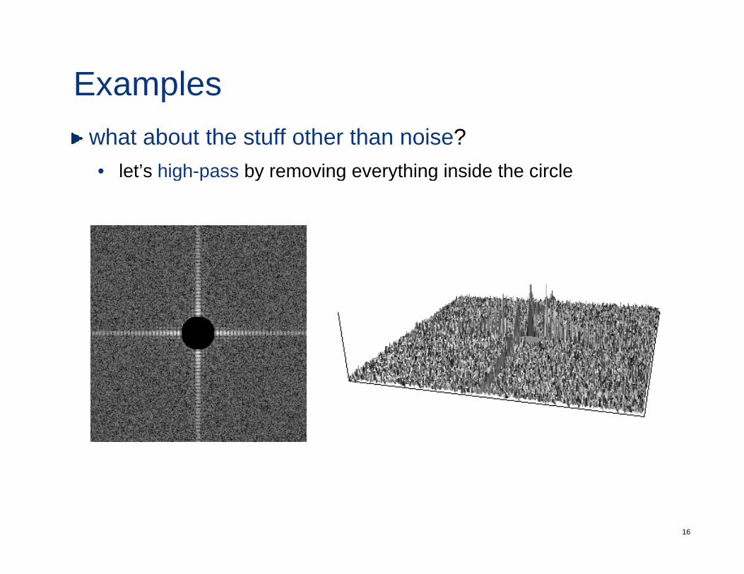
Exampleswhat about the stuff other than noise?• let’s high-pass by removing everything inside the circleg p y g y g

16

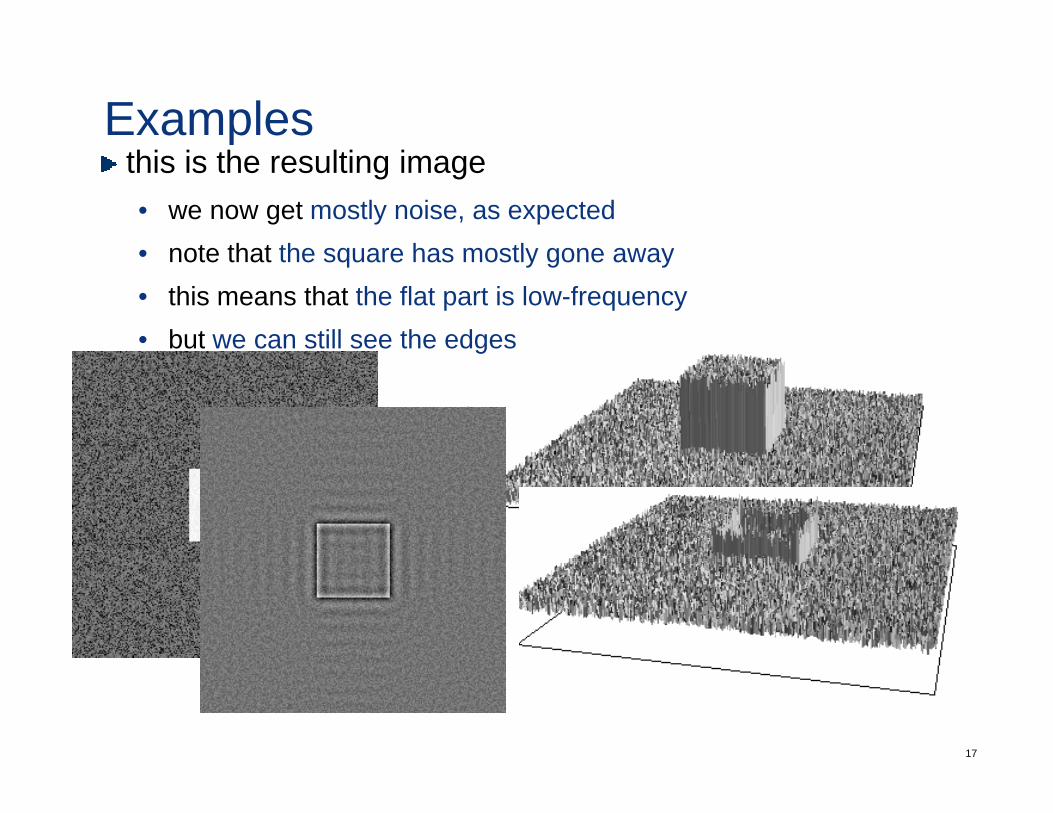
Exampleshi i h l i ithis is the resulting image• we now get mostly noise, as expected• note that the square has mostly gone away• note that the square has mostly gone away• this means that the flat part is low-frequency• but we can still see the edges

17

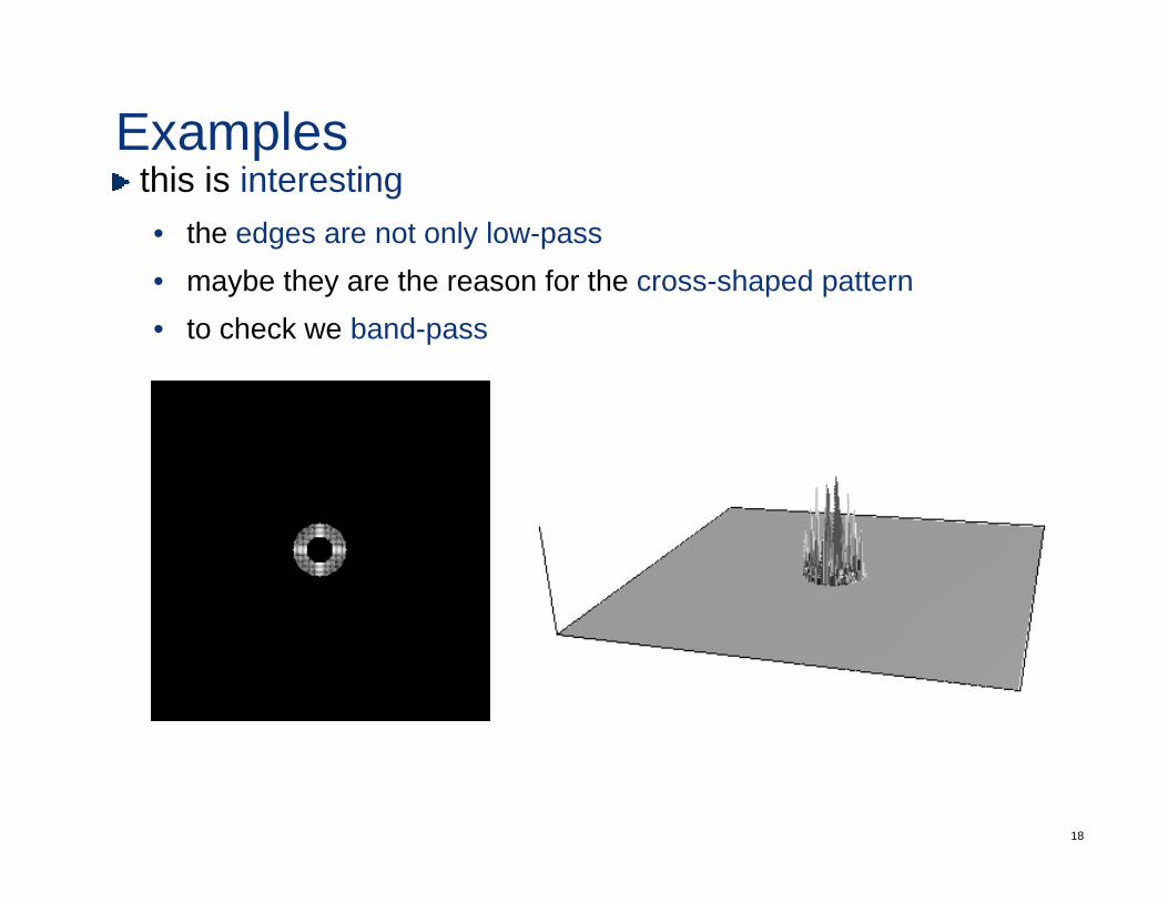
Exampleshi i i ithis is interesting• the edges are not only low-pass• maybe they are the reason for the cross shaped pattern• maybe they are the reason for the cross-shaped pattern• to check we band-pass

18

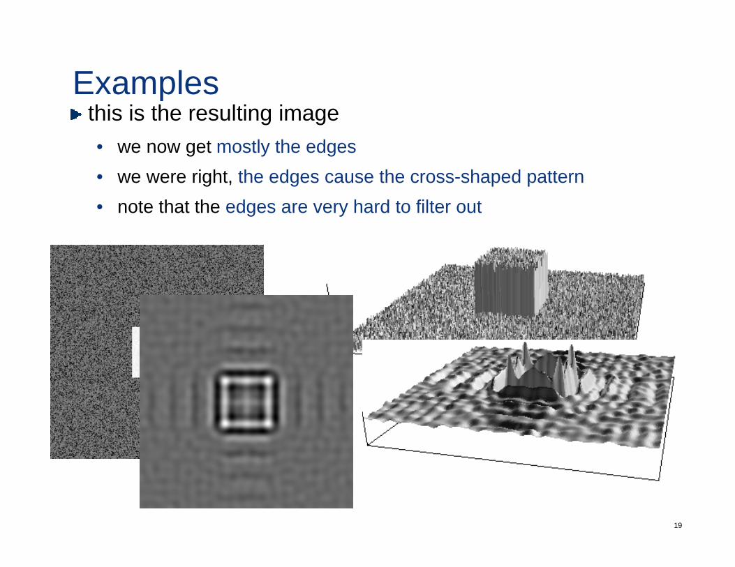
Exampleshi i h l i ithis is the resulting image• we now get mostly the edges• we were right the edges cause the cross shaped pattern• we were right, the edges cause the cross-shaped pattern• note that the edges are very hard to filter out

19

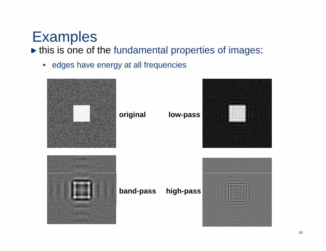
Exampleshi i f h f d l i f ithis is one of the fundamental properties of images:• edges have energy at all frequencies

original low-pass

band-pass high-pass

20

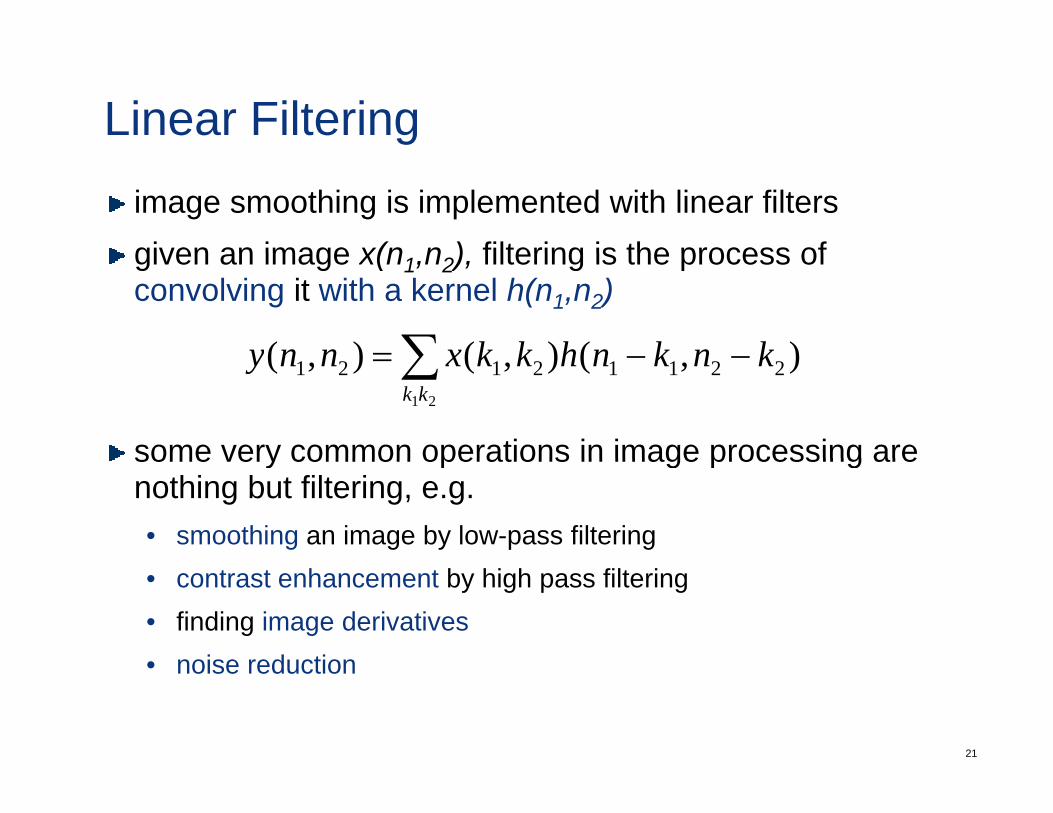
Linear Filteringimage smoothing is implemented with linear filtersgiven an image x(n n ) filtering is the process ofgiven an image x(n1,n2), filtering is the process ofconvolving it with a kernel h(n1,n2)

)()()( knknhkkxnny = ∑

some very common operations in image processing are

),(),(),( 2211212121

knknhkkxnnykk

−−= ∑

some very common operations in image processing are nothing but filtering, e.g.• smoothing an image by low-pass filtering• contrast enhancement by high pass filtering• finding image derivatives• noise reduction

21

• noise reduction

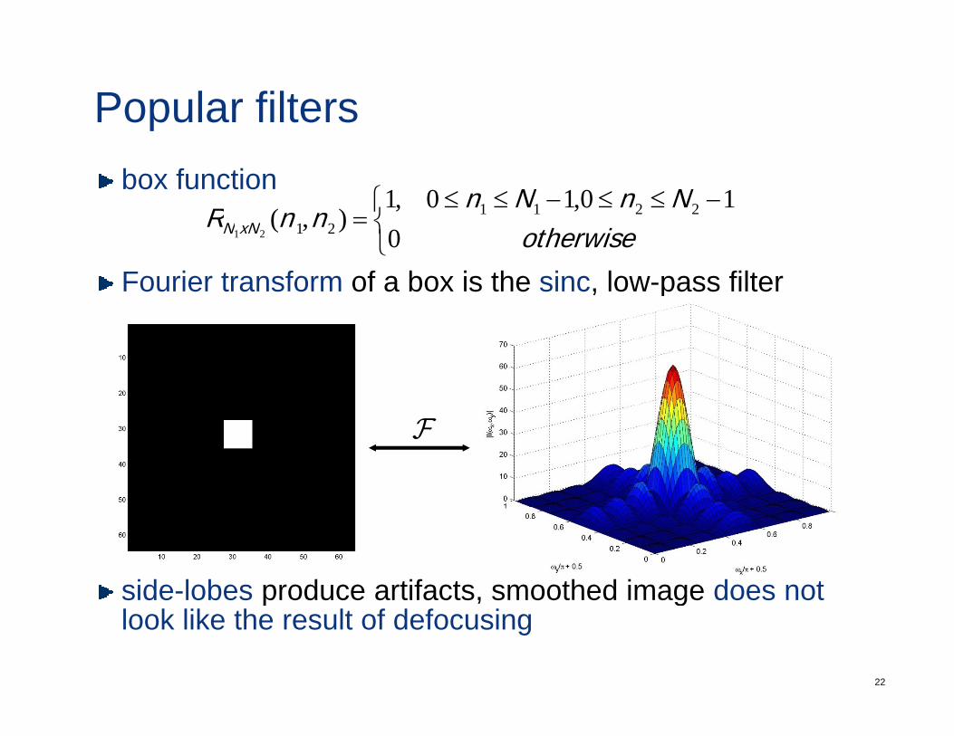
Popular filtersbox function

⎨⎧ −≤≤−≤≤

=th i

NnNnnnR xNN

10,10,1),( 2211

21

Fourier transform of a box is the sinc, low-pass filter⎩⎨ otherwisexNN 0

),( 2121

F

side-lobes produce artifacts, smoothed image does not

22

s de obes p oduce a ac s, s oo ed age does olook like the result of defocusing

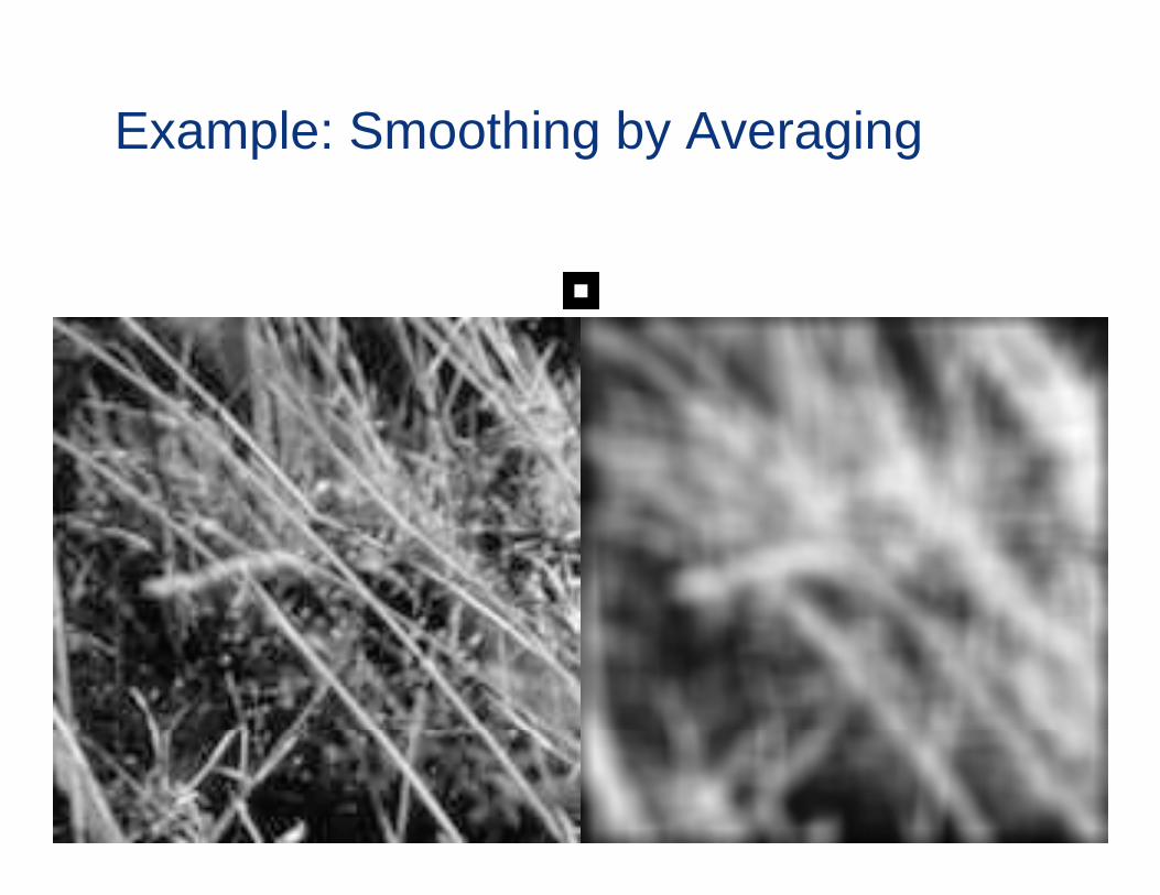
Example: Smoothing by Averaging

23

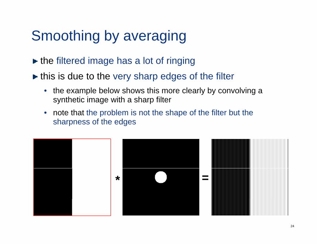
Smoothing by averagingthe filtered image has a lot of ringingthis is due to the very sharp edges of the filterthis is due to the very sharp edges of the filter• the example below shows this more clearly by convolving a

synthetic image with a sharp filter• note that the problem is not the shape of the filter but the

sharpness of the edges

* =

24

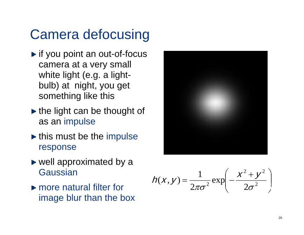
Camera defocusingif you point an out-of-focus camera at a very small

hite light (e g a lightwhite light (e.g. a light-bulb) at night, you get something like thisthe light can be thought of as an impulsethis must be the impulse responsewell approximated by awell approximated by a Gaussianmore natural filter for ⎟⎟

⎠

⎞⎜⎜⎝

⎛ +−= 2

22

2 2exp

21),(

σπσyxyxh

25

image blur than the box⎠⎝

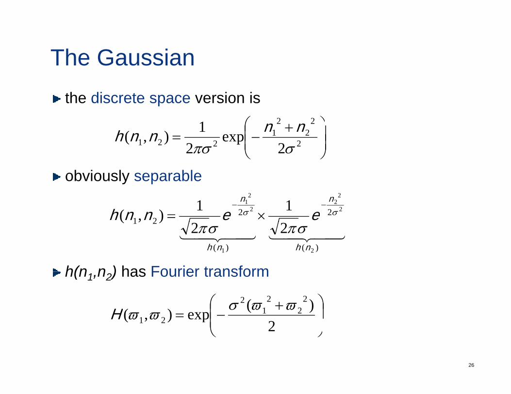
The Gaussianthe discrete space version is

⎞⎛ 221

b i l bl

⎟⎟⎠

⎞⎜⎜⎝

⎛ +−= 2

22

21

221 2exp

21),(

σπσnnnnh

obviously separable

2221

2

22

2

21 11),(

nn

eennh σσ−−

×=

h(n n ) has Fourier transform

44344214434421)()(

21

21

22),(

nhnh

σπσπ

h(n1,n2) has Fourier transform

⎟⎞

⎜⎜⎛ +−=

2)(exp),(

22

21

2

21ϖϖσϖϖH

26

⎠⎜⎝ 2

p),( 21

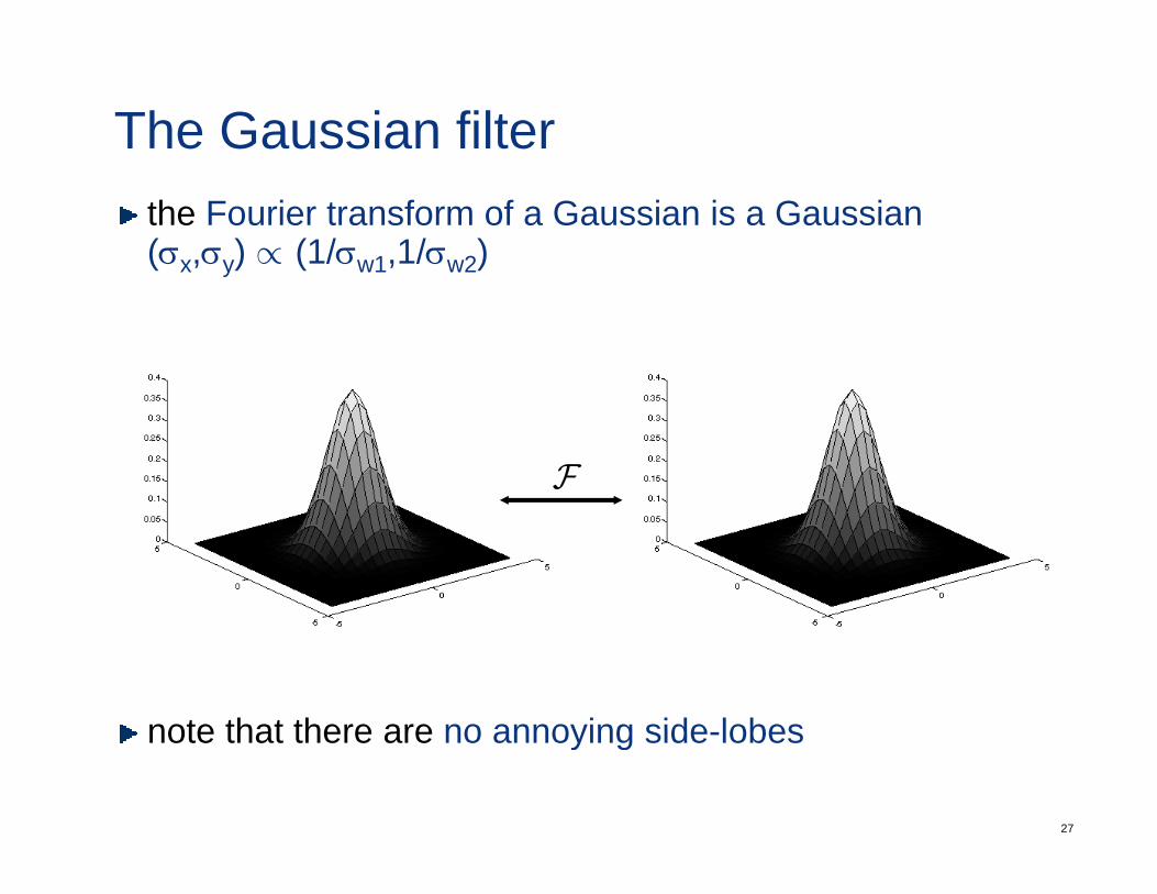
The Gaussian filterthe Fourier transform of a Gaussian is a Gaussian(σx,σy) ∝ (1/σw1,1/σw2)

F

note that there are no annoying side lobes

27

note that there are no annoying side-lobes

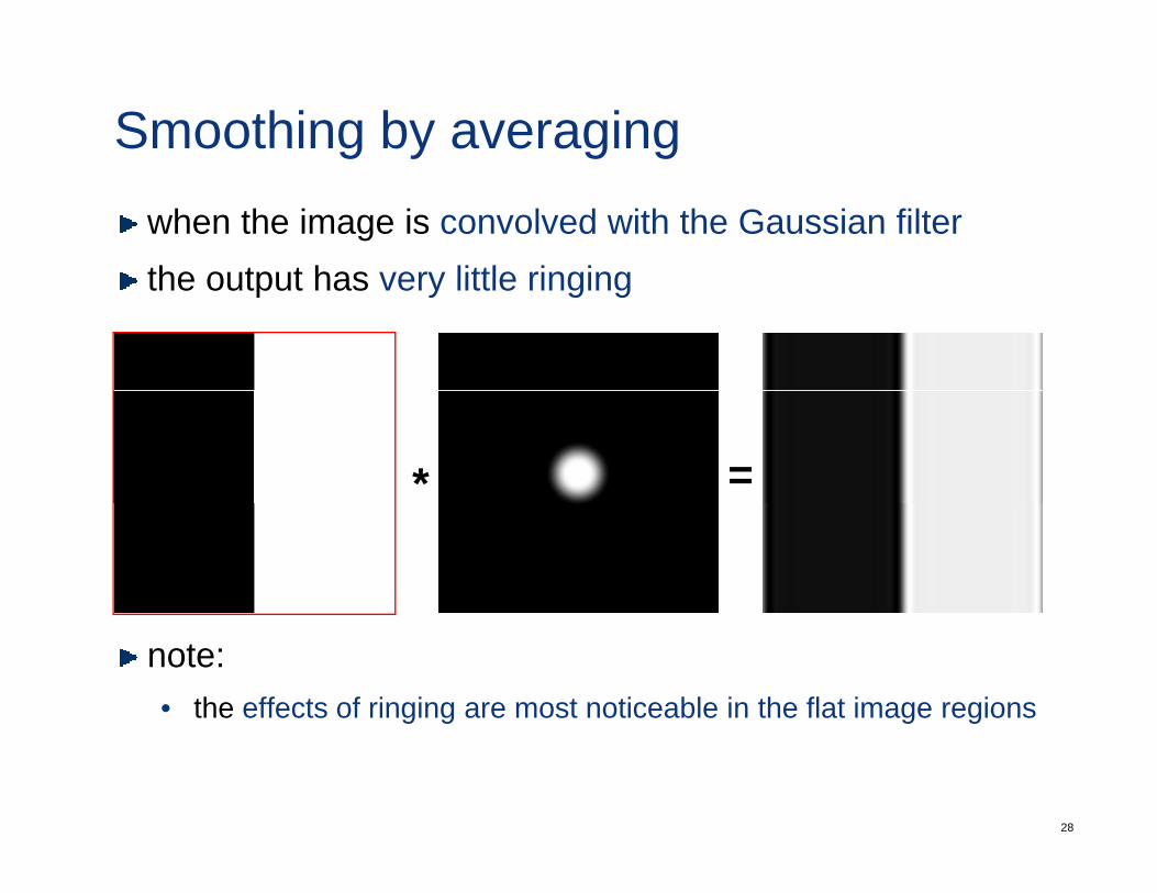
Smoothing by averagingwhen the image is convolved with the Gaussian filterthe output has very little ringingthe output has very little ringing

* =

note:• the effects of ringing are most noticeable in the flat image regions

28

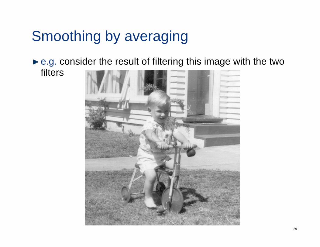
Smoothing by averaginge.g. consider the result of filtering this image with the two filters

29

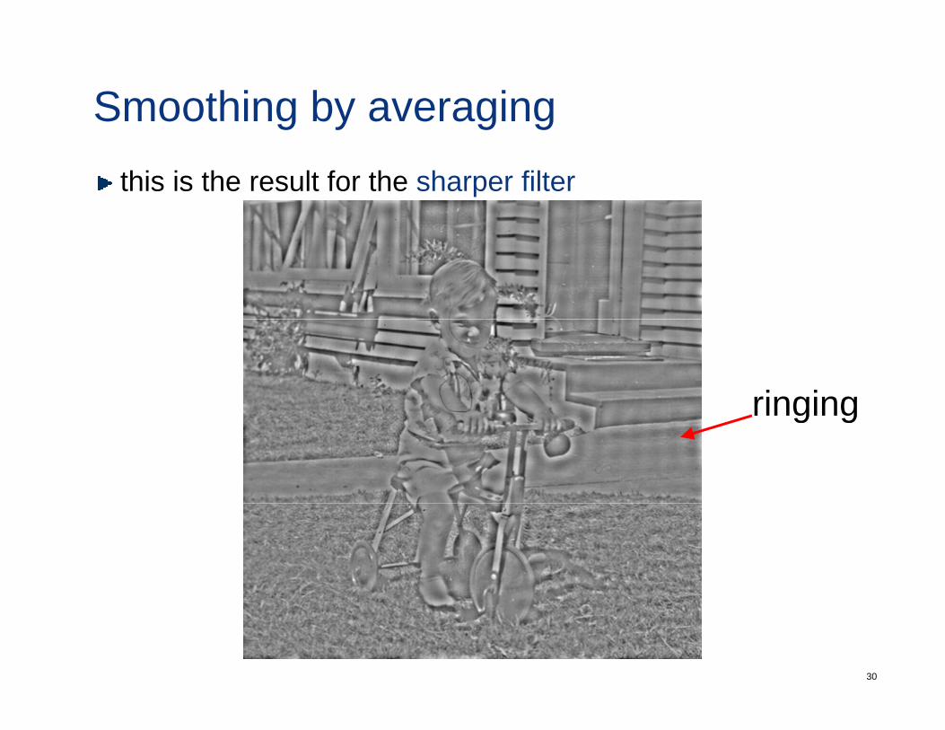
Smoothing by averagingthis is the result for the sharper filter

ringingringing

30

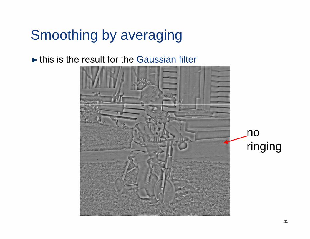
Smoothing by averagingthis is the result for the Gaussian filter

nono ringing

31

Smoothing by Averaging

32

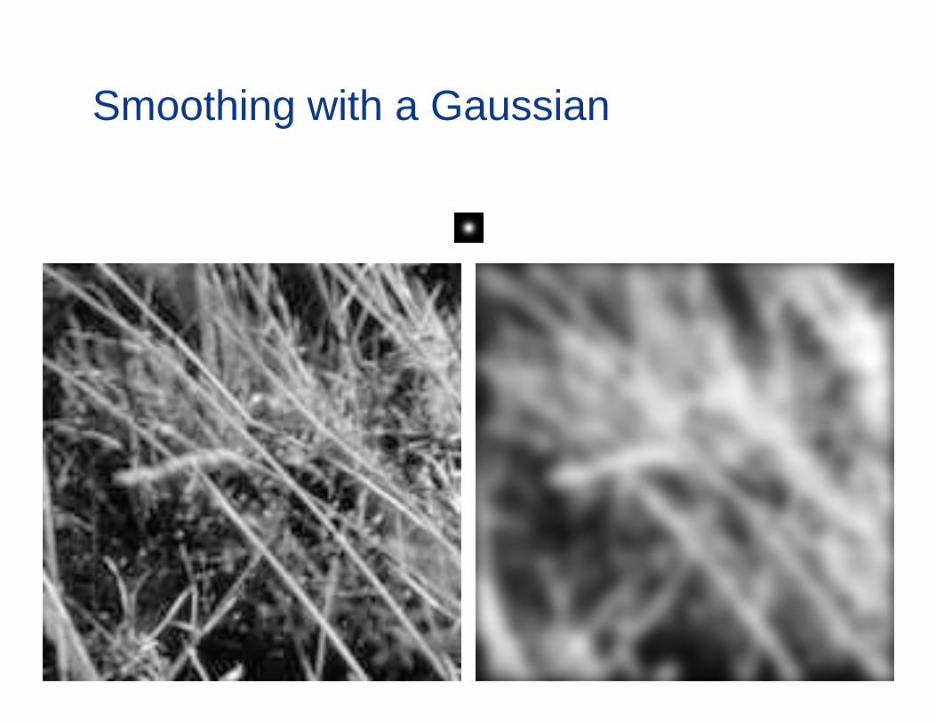
Smoothing with a Gaussian

33

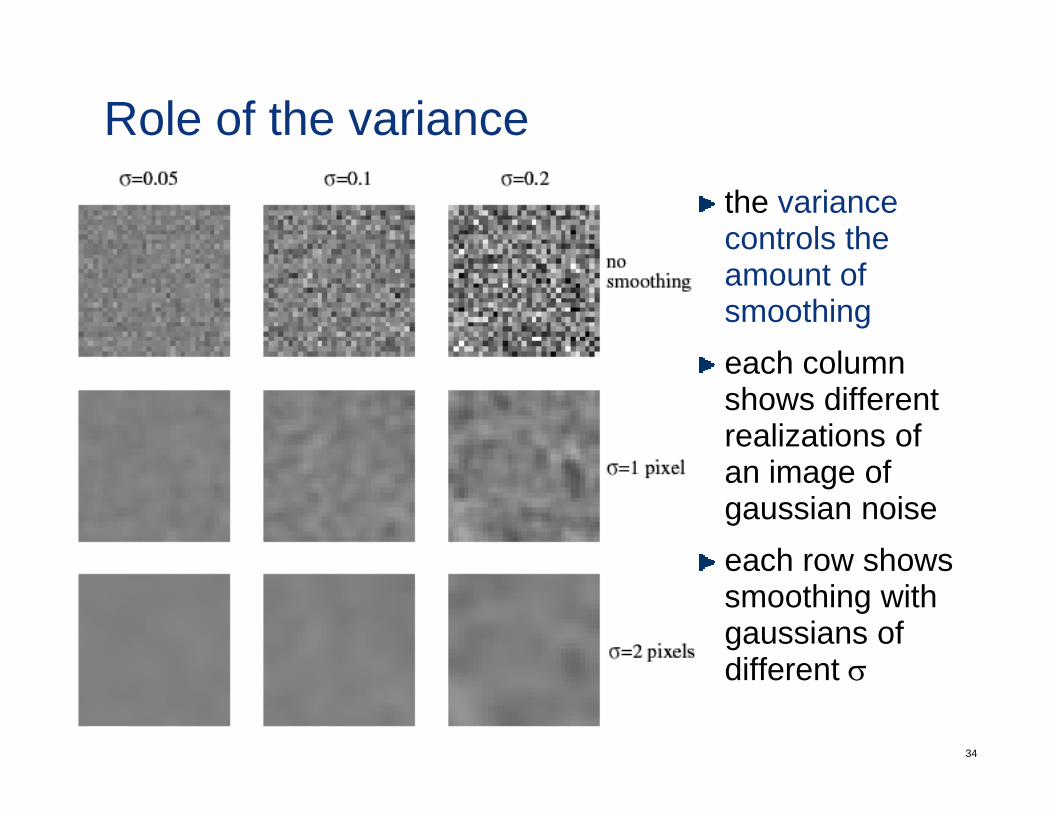
Role of the variancethe variance controls the amount of smoothing

h leach column shows different realizations of an image of gaussian noiseeach row showseach row shows smoothing with gaussians of diff t

34

different σ

Gradients and edgesfor image understanding, one of the problems is that there is too much information in an image just smoothing is not good enoughhow to detect important (most informative) image points?note that derivatives are large at points of great change• changes in reflectance (e.g. checkerboard pattern)• change in object (an object boundary is different from background)• change in object (an object boundary is different from background)• change in illumination (the boundary of a shadow)

these are usually called edge pointsdetecting them could be useful for various problems• segmentation: we want to know what are object boundaries

35

• recognition: cartoons are easy to recognize and terribly efficient to transmit

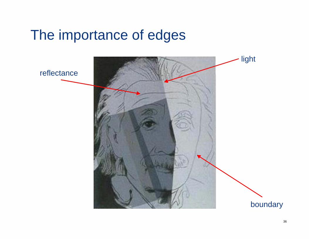
The importance of edgeslight

reflectancereflectance

36

boundary

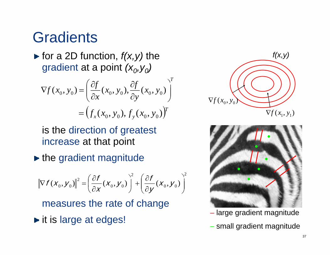
Gradientsfor a 2D function, f(x,y) the gradient at a point (x0,y0)

T⎞⎛

f(x,y)

T

yxyfyx

xfyxf ⎟⎟

⎠

⎞⎜⎜⎝

⎛∂∂

∂∂

=∇ ),(),,(),( 000000

( )Tff )()(),( 00 yxf∇

)(f∇

is the direction of greatest increase at that point

( )yx yxfyxf ),(),,( 0000= ),( 11 yxf∇

increase at that pointthe gradient magnitude

22 ⎞⎛ ∂⎞⎛ ∂ ff

measures the rate of change

00

2

002

00 ),(),(),( ⎟⎟⎠

⎞⎜⎜⎝

⎛∂∂

+⎟⎠⎞

⎜⎝⎛∂∂

=∇ yxyfyx

xfyxf

37

git is large at edges!

– large gradient magnitude

– small gradient magnitude

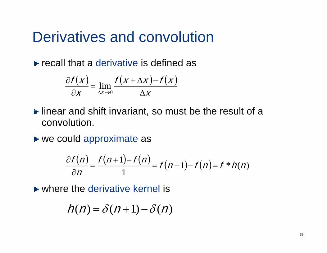
Derivatives and convolutionrecall that a derivative is defined as

( ) ( ) ( )xfxxfxf ∆+∂

linear and shift invariant so must be the result of a

( ) ( ) ( )x

xfxxfxxf

x ∆−∆+

=∂

∂→∆ 0

lim

linear and shift invariant, so must be the result of a convolution.we could approximate aspp

( ) ( ) ( ) ( ) ( ) )(*11

1 nhfnfnfnfnfnnf

=−+=−+

=∂

∂

where the derivative kernel is

1n∂

)()1()( nnnh δδ

38

)()1()( nnnh δδ −+=

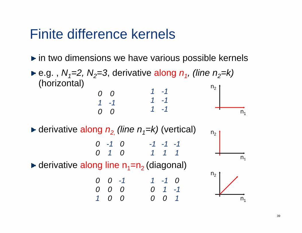
Finite difference kernelsin two dimensions we have various possible kernelse g N =2 N =3 derivative along n (line n =k)e.g. , N1=2, N2=3, derivative along n1, (line n2=k)(horizontal)

0 01 1

1 -11 -1

n2

derivative along n2 (line n1=k) (vertical)

1 -10 0

1 11 -1 n1

nderivative along n2, (line n1 k) (vertical)0 -1 00 1 0

-1 -1 -11 1 1 n1

n2

derivative along line n1=n2 (diagonal)0 0 -10 0 0

1 -1 00 1 -1

n2

39

0 0 01 0 0

0 1 -10 0 1 n1

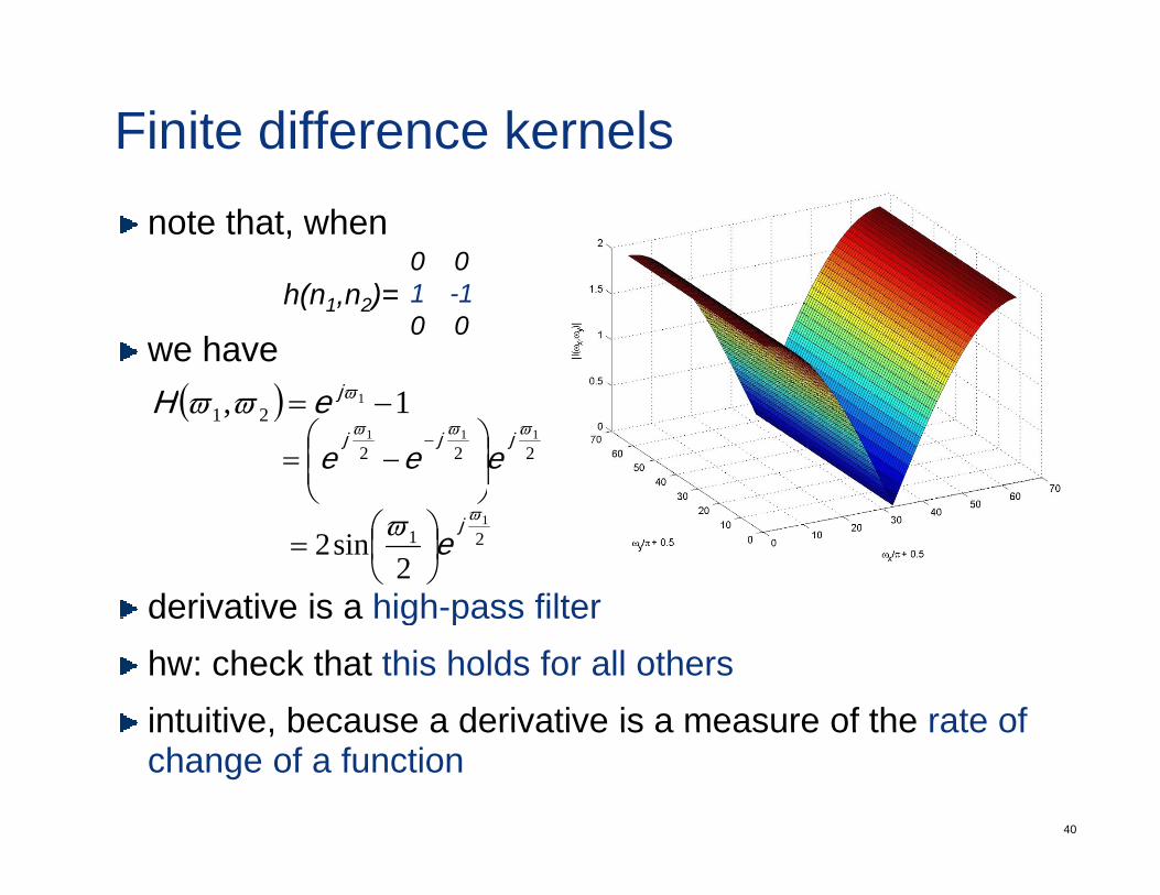
Finite difference kernelsnote that, when

0 0h(n1,n2)=

we have

1 -10 0

( ) 1ϖjH222

111 ϖϖϖ jjjeee ⎟⎟⎠

⎞⎜⎜⎝

⎛−=

−

( ) 1, 121 −= ϖϖϖ jeH

derivative is a high-pass filter

211

2sin2

ϖϖ je⎟⎠⎞

⎜⎝⎛=

derivative is a high pass filterhw: check that this holds for all othersintuitive, because a derivative is a measure of the rate of

40

intuitive, because a derivative is a measure of the rate of change of a function

64