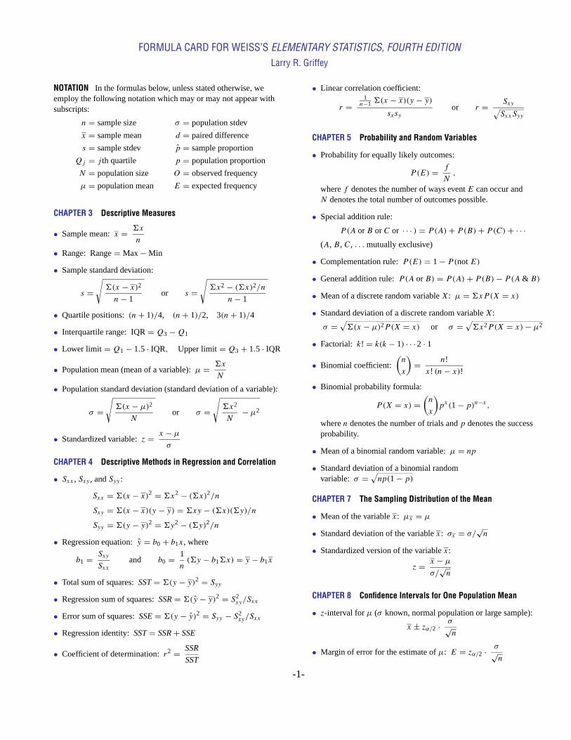
FORMULA CARD FOR WEISS’S ELEMENTARY STATISTICS, FOURTH EDITIONLarry R. Griffey

NOTATION In the formulas below, unless stated otherwise, weemploy the following notation which may or may not appear withsubscripts:

n H sample size

x H sample mean

s H sample stdev

Qj H j th quartile

N H population size

µ H population mean

σ H population stdev

d H paired difference

p H sample proportion

p H population proportion

O H observed frequency

E H expected frequency

CHAPTER 3 Descriptive Measures

• Sample mean:x H 6x

n

• Range: RangeH Max−Min

• Sample standard deviation:

s H√6(x − x)2n− 1

or s H√6x2 − (6x)2/n

n− 1

• Quartile positions:(n+ 1)/4, (n+ 1)/2, 3(n+ 1)/4

• Interquartile range: IQRH Q3 −Q1

• Lower limit H Q1 − 1.5 · IQR, Upper limitH Q3 + 1.5 · IQR

• Population mean (mean of a variable):µ H 6x

N

• Population standard deviation (standard deviation of a variable):

σ H√6(x − µ)2

Nor σ H

√6x2

N− µ2

• Standardized variable:z H x − µσ

CHAPTER 4 Descriptive Methods in Regression and Correlation

• Sxx , Sxy , andSyy :

Sxx H 6(x − x)2 H 6x2 − (6x)2/nSxy H 6(x − x)(y − y) H 6xy − (6x)(6y)/nSyy H 6(y − y)2 H 6y2 − (6y)2/n

• Regression equation:y H b0 + b1x, where

b1 H Sxy

Sxxand b0 H 1

n(6y − b16x) H y − b1x

• Total sum of squares:SSTH 6(y − y)2 H Syy• Regression sum of squares:SSRH 6(y − y)2 H S2

xy/Sxx

• Error sum of squares:SSEH 6(y − y)2 H Syy − S2xy/Sxx

• Regression identity:SSTH SSR+ SSE

• Coefficient of determination:r2 H SSR

SST

• Linear correlation coefficient:

r H1n−1 6(x − x)(y − y)

sxsyor r H Sxy√

SxxSyy

CHAPTER 5 Probability and Random Variables

• Probability for equally likely outcomes:

P(E) H f

N,

wheref denotes the number of ways eventE can occur andN denotes the total number of outcomes possible.

• Special addition rule:

P(A orB orC or · · · ) H P(A)+ P(B)+ P(C)+ · · ·(A, B, C, . . . mutually exclusive)

• Complementation rule:P(E) H 1− P(notE)

• General addition rule:P(A orB) H P(A)+ P(B)− P(A & B)

• Mean of a discrete random variableX: µ H 6xP(X H x)• Standard deviation of a discrete random variableX:

σ H√6(x − µ)2P(X H x) or σ H

√6x2P(X H x)− µ2

• Factorial: k! H k(k − 1) · · ·2 · 1

• Binomial coefficient:

(n

x

)H n!

x! (n− x)!• Binomial probability formula:

P(X H x) H(n

x

)px(1− p)n−x ,

wheren denotes the number of trials andp denotes the successprobability.

• Mean of a binomial random variable:µ H np• Standard deviation of a binomial random

variable: σ H√np(1− p)

CHAPTER 7 The Sampling Distribution of the Mean

• Mean of the variablex: µx H µ• Standard deviation of the variablex: σx H σ/

√n

• Standardized version of the variablex:

z H x − µσ/√n

CHAPTER 8 Confidence Intervals for One Population Mean

• z-interval forµ (σ known, normal population or large sample):

x ± zα/2 · σ√n

• Margin of error for the estimate ofµ: E H zα/2 · σ√n

-1-

FORMULA CARD FOR WEISS’S ELEMENTARY STATISTICS, FOURTH EDITIONLarry R. Griffey

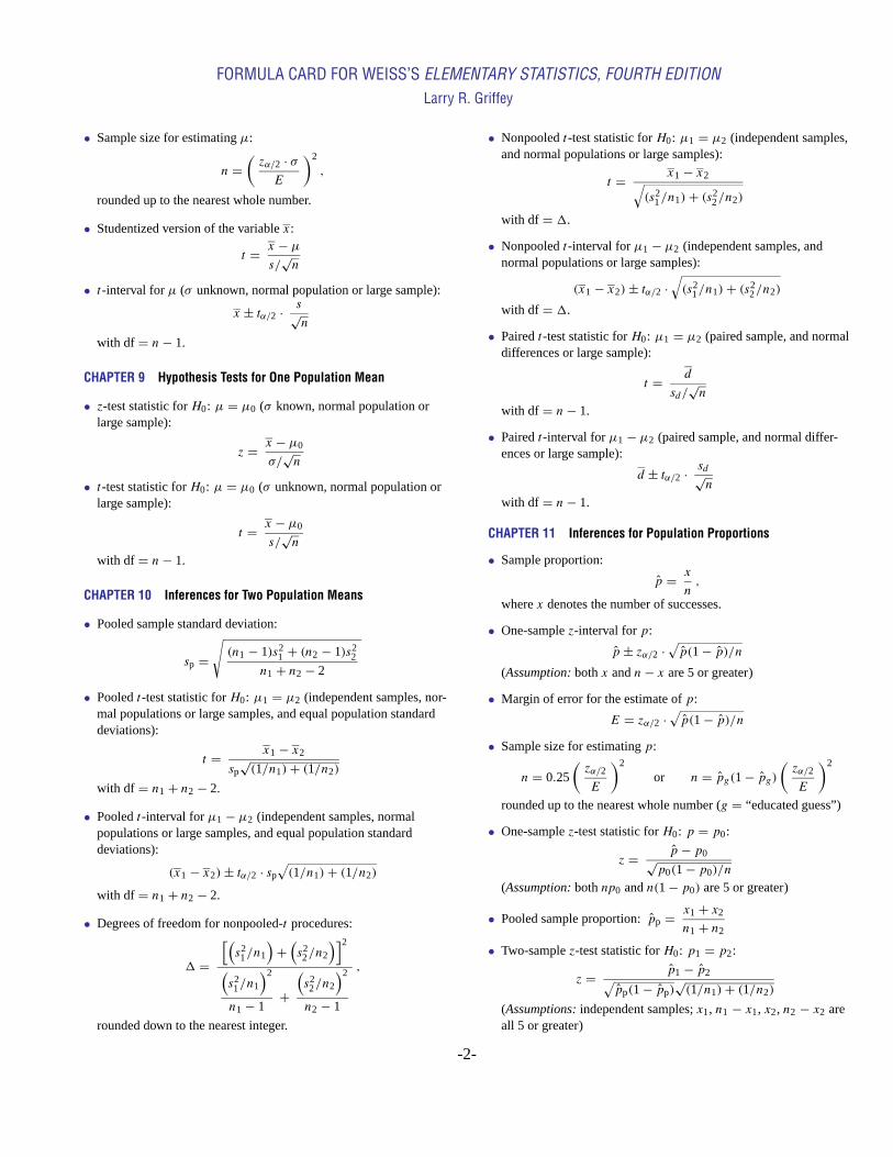
• Sample size for estimatingµ:

n H(zα/2 · σE

)2

,

rounded up to the nearest whole number.

• Studentized version of the variablex:

t H x − µs/√n

• t-interval forµ (σ unknown, normal population or large sample):

x ± tα/2 · s√n

with df H n− 1.

CHAPTER 9 Hypothesis Tests for One Population Mean

• z-test statistic forH0: µ H µ0 (σ known, normal population orlarge sample):

z H x − µ0

σ/√n

• t-test statistic forH0: µ H µ0 (σ unknown, normal population orlarge sample):

t H x − µ0

s/√n

with df H n− 1.

CHAPTER 10 Inferences for Two Population Means

• Pooled sample standard deviation:

sp H√(n1 − 1)s2

1 + (n2 − 1)s22

n1 + n2 − 2

• Pooledt-test statistic forH0: µ1 H µ2 (independent samples, nor-mal populations or large samples, and equal population standarddeviations):

t H x1 − x2

sp√(1/n1)+ (1/n2)

with df H n1 + n2 − 2.

• Pooledt-interval forµ1 − µ2 (independent samples, normalpopulations or large samples, and equal population standarddeviations):

(x1 − x2)± tα/2 · sp√(1/n1)+ (1/n2)

with df H n1 + n2 − 2.

• Degrees of freedom for nonpooled-t procedures:

1 H[(s21/n1

)+(s22/n2

)]2

(s21/n1

)2

n1 − 1+(s22/n2

)2

n2 − 1

,

rounded down to the nearest integer.

• Nonpooledt-test statistic forH0: µ1 H µ2 (independent samples,and normal populations or large samples):

t H x1 − x2√(s2

1/n1)+ (s22/n2)

with df H 1.

• Nonpooledt-interval forµ1 − µ2 (independent samples, andnormal populations or large samples):

(x1 − x2)± tα/2 ·√(s2

1/n1)+ (s22/n2)

with df H 1.

• Pairedt-test statistic forH0: µ1 H µ2 (paired sample, and normaldifferences or large sample):

t H d

sd/√n

with df H n− 1.

• Pairedt-interval forµ1 − µ2 (paired sample, and normal differ-ences or large sample):

d ± tα/2 · sd√n

with df H n− 1.

CHAPTER 11 Inferences for Population Proportions

• Sample proportion:

p H x

n,

wherex denotes the number of successes.

• One-samplez-interval forp:

p ± zα/2 ·√p(1− p)/n

(Assumption:bothx andn− x are 5 or greater)

• Margin of error for the estimate ofp:

E H zα/2 ·√p(1− p)/n

• Sample size for estimatingp:

n H 0.25

(zα/2

E

)2

or n H pg(1− pg)(zα/2

E

)2

rounded up to the nearest whole number (g H “educated guess”)

• One-samplez-test statistic forH0: p H p0:

z H p − p0√p0(1− p0)/n

(Assumption:bothnp0 andn(1− p0) are 5 or greater)

• Pooled sample proportion:pp H x1 + x2

n1 + n2

• Two-samplez-test statistic forH0: p1 H p2:

z H p1 − p2√pp(1− pp)

√(1/n1)+ (1/n2)

(Assumptions:independent samples;x1, n1 − x1, x2, n2 − x2 areall 5 or greater)

-2-

FORMULA CARD FOR WEISS’S ELEMENTARY STATISTICS, FOURTH EDITIONLarry R. Griffey

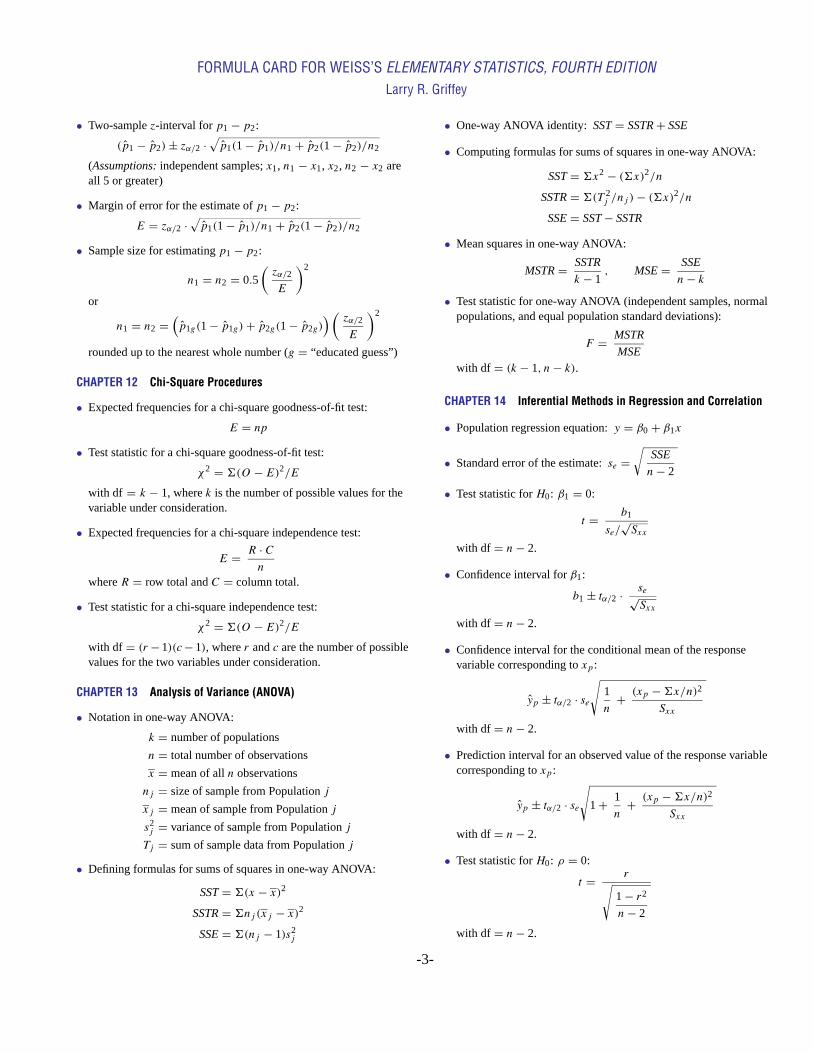
• Two-samplez-interval forp1 − p2:

(p1 − p2)± zα/2 ·√p1(1− p1)/n1 + p2(1− p2)/n2

(Assumptions:independent samples;x1, n1 − x1, x2, n2 − x2 areall 5 or greater)

• Margin of error for the estimate ofp1 − p2:

E H zα/2 ·√p1(1− p1)/n1 + p2(1− p2)/n2

• Sample size for estimatingp1 − p2:

n1 H n2 H 0.5

(zα/2

E

)2

or

n1 H n2 H(p1g(1− p1g)+ p2g(1− p2g)

)( zα/2E

)2

rounded up to the nearest whole number (g H “educated guess”)

CHAPTER 12 Chi-Square Procedures

• Expected frequencies for a chi-square goodness-of-fit test:

E H np• Test statistic for a chi-square goodness-of-fit test:

χ2 H 6(O − E)2/Ewith df H k − 1, wherek is the number of possible values for thevariable under consideration.

• Expected frequencies for a chi-square independence test:

E H R · Cn

whereR H row total andC H column total.

• Test statistic for a chi-square independence test:

χ2 H 6(O − E)2/Ewith df H (r −1)(c−1), wherer andc are the number of possiblevalues for the two variables under consideration.

CHAPTER 13 Analysis of Variance (ANOVA)

• Notation in one-way ANOVA:

k H number of populations

n H total number of observations

x H mean of alln observations

nj H size of sample from Populationj

xj H mean of sample from Populationj

s2j H variance of sample from Populationj

Tj H sum of sample data from Populationj

• Defining formulas for sums of squares in one-way ANOVA:

SSTH 6(x − x)2SSTRH 6nj (xj − x)2

SSEH 6(nj − 1)s2j

• One-way ANOVA identity: SSTH SSTR+ SSE

• Computing formulas for sums of squares in one-way ANOVA:

SSTH 6x2 − (6x)2/nSSTRH 6(T 2

j /nj )− (6x)2/nSSEH SST− SSTR

• Mean squares in one-way ANOVA:

MSTRH SSTR

k − 1, MSEH SSE

n− k• Test statistic for one-way ANOVA (independent samples, normal

populations, and equal population standard deviations):

F H MSTR

MSEwith df H (k − 1, n− k).

CHAPTER 14 Inferential Methods in Regression and Correlation

• Population regression equation:y H β0 + β1x

• Standard error of the estimate:se H√

SSE

n− 2

• Test statistic forH0: β1 H 0:

t H b1

se/√Sxx

with df H n− 2.

• Confidence interval forβ1:

b1 ± tα/2 · se√Sxx

with df H n− 2.

• Confidence interval for the conditional mean of the responsevariable corresponding toxp :

yp ± tα/2 · se√

1

n+ (xp −6x/n)2

Sxx

with df H n− 2.

• Prediction interval for an observed value of the response variablecorresponding toxp :

yp ± tα/2 · se√

1+ 1

n+ (xp −6x/n)2

Sxx

with df H n− 2.

• Test statistic forH0: ρ H 0:

t H r√1− r2

n− 2

with df H n− 2.

-3-