Working Paper

BANK OF GREECE

FOREIGN EXCHANGE INTERVENTION AND EQUILIBRIUM

REAL EXCHANGE RATES

No. 56 February 2007

Dimitrios A. Sideris

BANK OF GREECE Economic Research Department – Special Studies Division 21, Ε. Venizelos Avenue GR-102 50 Αthens Τel: +30210-320 3610 Fax: +30210-320 2432 www.bankofgreece.gr Printed in Athens, Greece at the Bank of Greece Printing Works. All rights reserved. Reproduction for educational and non-commercial purposes is permitted provided that the source is acknowledged. ISSN 1109-6691

FOREIGN EXCHANGE INTERVENTION AND EQUILIBRIUM REAL EXCHANGE RATES

Dimitrios A. Sideris University of Ioannina and Bank of Greece

ABSTRACT

Monetary authorities intervene in the currency markets in order to pursue a monetary rule and/or to smooth exchange rate volatility caused by speculative attacks. In the present paper we investigate for possible intervention effects on the volatility of nominal exchange rates and the estimated equilibrium behaviour of real exchange rates. The main argument of the paper is that omission of intervention effects -when they are significant- would bias the ability to detect any PPP-based behaviour of the real exchange rates in the long run. Positive evidence for this argument comes from the experience of six Central and Eastern European economies, whose exchange markets are characterised by frequent interventions.

Keywords: foreign exchange market intervention; real exchange rates; PPP JEL classification: F31; C32; E58 Acknowledgements: I would like to thank H. Gibson, N. Mylonidis, and P. Petroulas for helpful comments and suggestions. All remaining errors are entirely my responsibility. The views expressed in this paper are the author’s own and do not necessarily represent those of the institutions to which he is affiliated.

Address for Correspondence: Dimitrios Sideris, Department of Economics, University of Ioannina, University Campus, 45110 Ioannina, Greece, Tel. +26510 - 95942 e-mail: disideri@cc.uoi.gr.

5

1. Introduction

Official intervention in the foreign exchange market is defined as official

purchases and sales of foreign exchange by the monetary authorities in order to affect

the exchange rate. The literature on intervention states that central banks intervene in

order (i) to correct misalignments or to stabilise the exchange rate at predetermined

targeted levels or within targeted rates of change (when, for example, they pursue a

monetary policy rule) and (ii) to address disorderly market conditions – mainly high

exchange rate volatility and/or sharp exchange rate fluctuations caused by speculative

bubbles phenomena.1 As a result, in the first case, interventions may cause the real

exchange rate to move in a target rate for long periods of time -and this can be

interpreted as equilibrium values which shift from time to time- whereas in the second

case, interventions may lead the exchange rate to move back to fundamental-based

levels and/or to adjust faster to its long-run equilibrium level (for similar arguments

see, inter alia, Sweeney, 1999).2

Whether or not intervention has an impact on exchange rates, offering the

authorities an independent policy tool for influencing the foreign exchange market is

an issue of great policy importance. As a consequence, intervention and its effects has

been the subject of a large number of empirical articles in the international economics

literature (see, inter alia, Baillie, 2000). The relevant empirical articles provide mixed

evidence on the effectiveness of official interventions in the currency markets. Early

empirical studies using data from the 1970s suggest that intervention operations have,

at most, a short-lived influence on exchange rates (see the survey in Dominguez and

Frankel, 1993a), whereas more recent studies indicate that intervention influences

both the level and variance of exchange rates (for a survey of the articles written till

the mid 1990s, see Sarno and Taylor, 2002a). Most recent empirical studies (written

from the mid 1990s on) tend to agree that there exists a significant effect of the

monetary authorities’ intervention at least on the short-run dynamics of the exchange

rates. Empirical evidence is based on advanced country experience, mainly the US,

1 We use the standard definition of intervention which focuses on exchange rate-related objectives and not the definition used by Canales-Kriljenko et al. (2003) which also accounts for operations to accumulate and supply foreign exchange to the market. 2 For a survey of the literature on theoretical and policy issues concerning intervention see inter alia Canales-Kriljenko et al. (2003) and Sarno and Taylor (2002a).

6

Germany (and the EU), Japan and Australia, given that data on central bank

operations are available for these countries.3

Alongside the studies on intervention, a vast empirical literature on the

behaviour of the real exchange rates and the validity of purchasing power parity (PPP)

has grown up during the last three decades or so and by now constitutes a great body

of the international finance literature. Most recent studies use the concept of

stationarity and cointegration to test for PPP. They raise the low power problem of the

early studies, which is attributed to short sample sizes and the low statistical power of

the early tests, and advocate the use of advanced econometric techniques (for a

survey, see, inter alia, Sarno and Taylor, 2002b). Within this strand of the empirical

literature, two recent studies raise the argument that the empirical inability to detect

stationarity of the real exchange rate or some version of PPP may be due to the effects

of interventions by the monetary authorities in the currency markets.4 In particular,

Taylor (2004) argues that intervention operations result in non-linear dynamics for the

real exchange rate. He develops a regime switching model, in which the transition

probabilities of switching between stable and unstable regimes depend upon

intervention activity, the extent of exchange rate misalignment and the duration of the

regime. The estimation of a Markov-switching model for the real DM/US$ rate

provides results favourable to his arguments.

Based on a somewhat similar idea, Brissimis, Sideris and Voumvaki (2005)

argue that long-run PPP is not likely to be evidenced for economies in which the

monetary authorities intervene in the exchange rate market to support a certain

exchange rate rule. They claim that policy behaviour affects the short-run adjustment

to PPP and the ability to uncover long-run PPP empirically, even when PPP holds.

Their analysis is based on a simple theoretical model in which short-run intervention

3 In particular: Positive evidence for the effectiveness of intervention strategies on the US$/DM exchange rate volatility is presented in Dominguez and Frankel (1993b), Bonser-Neal and Tanner (1996), Hung (1997), Dominguez (1998), Fatum and Hutchison (2003a). Support for the effectiveness of intervention and monetary policies on the dynamics of the US$/yen rate is provided by Bonser-Neal and Tanner (1996), Hung (1997), Dominguez (1998), Fatum and Hutchison (2003b), Brissimis and Chionis (2004) and Frenkel et al. (2005). Bonser-Neal et al. (1998) find that the US$ exchange rates respond immediately to US monetary policy actions. Usman and Savvides (1994) indicate that French intervention does not exert a significant influence on the FF/DM rate. Intervention is shown to be associated with the volatility (Edison et al., 2003) and the conditional variance of the return (Kim et al., 2000) of the Australian $/US$ rate. Aguilar and Nydahl (2000) provide weak support for the effects of intervention on the level and the volatility of the Swedish krona /US$ rate. 4 Actually, the idea that foreign exchange market intervention may prevent an exchange rate from always being at its PPP-defined value goes back to Cassel (see Officer, 1976).

7

strategies target a particular value for the real exchange rate which does not

necessarily equal the PPP rate. Positive evidence for their arguments comes mainly

from the experience of the Greek economy.

In a paper belonging to a related strand of the literature, which investigates the

source of shocks to real and nominal exchange rates (see, inter alia, Clarida and Gali,

1994), Kim (2003) comes up with similar suggestions. Kim analyses jointly the

effects of foreign exchange intervention strategies –pursued by setting exchange

reserves- and monetary policy on the exchange rate. He finds that foreign exchange

policy shocks have substantial effects on the exchange rate, which are even more

important sources of exchange rate fluctuations than conventional monetary policy

shocks. He argues that it is important to model foreign exchange intervention

explicitly in the study of exchange rate behaviour.

In the present paper, we extend this nascent literature by investigating possible

intervention effects on the volatility of the exchange rates and the estimated long-run

behaviour of exchange rates with respect to that of domestic and foreign prices, using

data from six Central and Eastern European Countries (CEEC) in transition. We first

examine the importance of intervention policies on the dynamics of exchange rates,

and secondly, once the significance of these policies is indicated, we investigate

whether the omission of intervention effects biases our ability to detect any

fundamental-based behaviour of the exchange rates in the long run. When the

monetary authorities intervene in the foreign exchange markets to influence the

behaviour of the exchange rates, the exchange rates reaches levels that would not

reach if left to be influenced by goods market forces alone. Central banks may

intervene to stabilise the exchange rate at a targeted level, which does not necessarily

equal the PPP level, when they support a certain exchange rate rule. They may also

intervene in order to make the exchange rate revert to an assumed equilibrium -

‘mean’- level, which, nevertheless, may not equal the equilibrium level implied by the

effects of market forces. Thus, we advocate that in order to detect any equilibrium

relationship connecting prices and exchange rates, as formed by market forces alone,

we should first identify and isolate effects exerted from intervention operations –

which are exogenous to the goods market arbitrage- on the short-run dynamics of the

exchange rates.5 This idea is in turn based on the well-known argument in the 5 This argument is in line with the suggestions of Brissimis et al. (2005).

8

empirical economics literature using cointegration techniques, which states that the

explicit specification of the short-run dynamics is crucial for a successful estimation

of the long-run relations of the variables of interest (see, inter alia, Juselius, 1995).

The rest of the paper is organised as follows: Section 2 presents the

specification of the theoretical arguments of the present study whereas section 3

provides information on the exchange rate policies pursued in the economies under

consideration. Section 4 presents the econometric methodology used. Section 5

reports the empirical analysis and the obtained results. The final section summarises

and concludes.

2. The theoretical specification

The point of the present work is that, by isolating the effects coming from

intervention strategies on the exchange rate dynamics, which can also be considered

as nominal shocks, we are then able to detect any equilibrium relationship connecting

prices and exchange rates as formed by market forces alone. The standard error

correction framework to test for any equilibrium relationship involving relative prices

and exchange rates based on market fundamentals is the following:

it

k

iiit

k

iiit

k

iitt ppsppss −

=−

=−

=− ∆+∆+∆+−−−=∆ ∑∑∑ **))((

03

02

111211 λλλγγζ (1)

where ζ1<0. s, p and p* are the exchange rate, defined as units of domestic currency

per unit of foreign currency, the domestic and foreign price level respectively, all

expressed in logs, ∆ denotes the first difference operator and k denotes the number of

lags involved in the estimation. (1) implies that a PPP relation of the form s = γ1 + γ2

(p - p*) is valid in the long run.6 The first term on the right-hand side of (1) represents

short-run deviations from PPP which are corrected through time at a speed given by ζ1

and captures the influence of goods market arbitrage that tends to establish PPP in the

long run. The short-run behaviour of the exchange rate is also allowed to be

influenced by its own past values and current and past values of domestic and foreign

inflation as indicated by the rest of the terms of the right hand side of (1).

6 For γ2 =1, strong PPP is implied, which assumes one-to-one long-run proportionality between exchange rates and relative prices; γ2 ≠ 1 implies weak PPP which allows long-run proportionality to differ from unity in order to account for information and transportation costs and measurement errors.

9

In the present work, we advocate instead the use of a framework which

accounts for the effects of intervention – when they are significant – on the exchange

rate dynamics, of the form:

∆st =ζ2(s– γ1- γ2(p - p*))t-1 it

l

iit

k

iit

k

iit

k

i Rpps −=

−=

−=

−=

∆+∆+∆+∆+ ∑∑∑∑0

40

30

21

1 *ιιιι

λλλλ (2)

where ζ2 < 0. l denotes the number of lags involved in the estimation and R is the (net)

holdings of foreign assets by the central bank. The last term on the right hand side of

(2) captures the effects of current and past intervention, as approximated by ∆R.7

Intervention can alter the market adjustment path towards PPP by exerting an impact

on the exchange rate dynamics. More importantly, intervention can also affect the

estimated equilibrium relationship, in the event that central banks target the exchange

rate at a level other than the PPP level, as Brissimis et al. (2005) indicate.8

7 Changes in reserves may not correspond perfectly to interventions for a number of reasons (see Neely, 2000); they may also be measured with error. Nevertheless, their use has been a common strategy in the early empirical works on intervention (see Taylor, 1982; Szakmary and Mathur, 1997). In the present work, given the scarcity of data on interventions in the six economies, we use this variable to proxy intervention. 8 Brissimis et al. (2005) incorporate into the dynamics of a PPP-type exchange rate model the effects of intervention, approximated by ∆R, as following:

∆st = λ(s – α – (p - p*)) t-1 + µ∆Rt , λ<0 (B1) In (B1), the first term on the right-hand side expresses the market adjustment path to the equilibrium PPP of the form s=α + (p - p*), whereas the second term captures the effects of intervention. Brissimis et al. (2005) then assume that central banks determine intervention according to the policy rule: ∆Rt = k1(st – ts ) + k2∆st , k1, k2 < 0 (B2)

with ts = β0 + β1 (pt - p*t) (B3)

The policy rule (B2) implies that intervention operations aim to reduce deviations of the exchange rate from a target rate ( )s and at moderating exchange rate volatility. The target rate is set in terms of relative prices as shown in (B3) and need not be the PPP level; for example, for a country that uses its exchange rate as a disinflationary means, β1 < 1. Substituting (B2) and (B3) into (B1) yields: ∆st = λ(st-1 – α - pt-1 + p*

t-1) + µk1(st – β0 – β1 (pt - p*t)) + µk2∆st (B4)

which implies a static solution of the form: s=δ0 + δ1(p – p*) (B5) , with δ0 = (λα+µβ0)/(λ+µk1), δ1 = (λ+µk1β1)/(λ + µk1). Equation (B5) is not a long-run relationship since it incorporates short-run policy effects. As shown, δ1 is a function of the policy rule parameter β1 and would take the value 1 only if β1 = 1, i.e. the authorities follow a PPP rule; in the general case (for β1 ≠ 1), long-run PPP would not be accepted, even though it holds (as implied by B1). Thus, testing for any long-run relationship between exchange rates and relative prices while omitting the short-run effects from intervention, would introduce estimation bias to the parameters of the equilibrium relationship.

10

3. Exchange rate policies in the selected economies

The economies under consideration are those of Bulgaria, Poland, Romania,

Russia, Slovenia and Ukraine and the analysis covers the period following their

reforms to market economies at the beginning of the 1990s. The choice of the

particular sample of countries is motivated by two reasons. First, we consider that

intervention effects are likely to be important for the determination of the short-run

dynamics of the six exchange rates for three reasons. (i) All six countries have

adopted independently floating or managed floating exchange rate regimes in which

the central banks have lots of discretion over intervention policies.9 (ii) Despite the

fact that the central banks of the countries issuing international reserve currencies

rarely intervene anymore (with the exception of the Bank of Japan), those of the six

countries intervened actively in the foreign exchange market during the period

analysed (see Canales-Kriljenko et al., 2003). (iii) The central banks of the selected

economies intervene in amounts that are significant relative to both market turnover

and base money; moreover, a number of banking, monetary and foreign exchange

regulations existing in these countries constrict the market’s size, thus making the

central bank a more important player (see Canales-Kriljenko et al., 2003).10 Second,

no existing study using data from these six countries provides evidence for

stationarity of the real exchange rates, or the validity of any PPP version in the long

run.11

The monetary and exchange rate policies pursued in the six economies during

the period examined share a number of common features. Transition started in 1992 in

Russia and Ukraine and somewhat earlier in Bulgaria, Poland, Romania and Slovenia. 9 For this reason, we do not include in the present sample the economies of Slovakia and the Czech Republic, which pursued fixed pegs until 1996 and Hungary, which adopted a fixed peg until 1995 (see Hagen and Zhou, 2002). With a peg, intervention is obligatory (unless the peg is abandoned) rather than discretionary. 10 Actually, similar experiences are observed in some other economies of the former Soviet Union, which have also adopted managed floating exchange rate regimes; nevertheless we analyse the experience of the six selected economies, as data for these six economies go back to the early 1990s. 11 In particular: Thacker (1995) tests for stationarity of the real exchange rates of Poland and Hungary and rejects the hypothesis. Choudhry (1999) tests for cointegration between relative prices and nominal exchange rates of the currencies of Poland, Romania, Russia and Slovenia vis-a-vis the US$. He provides evidence of cointegration -but not of a PPP relationship- for Russia and Slovenia. Christev and Noorbakhsh (2000) test for PPP for Bulgaria, the Czech Republic, Hungary, Poland, Romania and Slovakia applying cointegration techniques; they find evidence for cointegrating relationships but not for PPP. Sideris (2006) investigates the validity of PPP for a panel of seventeen CEEC economies (which comprises the six economies of the present analysis) vis-à-vis the US. He applies cointegration

11

The process of economic transition began with a liberalisation of the foreign exchange

markets and the introduction of currency convertibility. These drastic steps resulted in

initial deep undervaluations of the national currencies. At the same time, price

liberalization was accompanied by very high inflation rates.

The countries adopted exchange rate regimes adequate for the specific

conditions of each economy. All countries in the sample started with a conventional

peg, but they moved to managed floating or intermediate regimes very soon.12

Bulgaria, Poland, Romania and Slovenia abandoned their pegs in 1991; Russia and

Ukraine in 1993. Slovenia adopted a managed float with no pre-announced path for

the exchange rate for the whole post-1991 period. Romania adopted a managed float

for the whole period, excluding the years 1992-1997, when it pursued an independent

float. Bulgaria adopted a managed float from 1991 until 1997, when it moved back to

a currency board agreement. Poland, Russia and Ukraine changed relatively often the

regime they pursued; they adopted diverse intermediate and floating regimes in

different sub-periods in the post-1991 period.13

For most economies, price stability has been the core monetary policy target

for most of the period and the authorities have pointed to the tight link between

inflation and the exchange rate as a key reason why they preferred relatively stable

exchange rates. Nevertheless, concern about the impact of an appreciation on

economic performance played also a role on the conduct of exchange rate policies.

This meant deciding whether any real currency appreciation was to be absorbed by

allowing the currency to appreciate in nominal terms or allowing prices to rise.

Priorities varied in different time periods, in the different countries. Thus, intervention

strategies at times were conducted to accommodate for the inflation differential and

maintain a stable real exchange rate, while at other times they let the real exchange

rate appreciate.

and panel cointegration techniques and offers support for long-run equilibria, but not for any PPP relationship. 12 Following Hagen and Zhou (2002), the exchange rate regimes can be classified to: (i) pegged regimes (dollar- and/or euro- izations, currency boards and conventional fixed pegs), (ii) floating regimes (managed floats with no preannounced path for the exchange rate and independent floats) and (iii) intermediate regimes (horizontal bands, crawling pegs and crawling bands). 13 We report the official regimes adopted by the economies. Even though adjustment in the central parities and foreign exchange market interventions can produce differences between the official regime and the de facto regime (see Calvo and Reinhart, 2002), we consider that official regimes guide financial market expectations about exchange rate developments and affect international financial policy decisions.

12

In the cases of Russia and Ukraine interest rate policies were not so important

for the conduct of monetary policy and to smooth exchange rate volatility; thus the

monetary and exchange rate policies were executed via foreign exchange market

operations. In all countries, interventions were the main policy tool for the conduct of

monetary policy for long periods and the authorities turned out to intervene often in

the markets. In certain periods the monthly volatility of reserves exceeded that of

nominal exchange rates (e.g. Poland for the period 1999-2002) being more than twice

that of the exchange rate in Russia and Ukraine for the period 1999-2002 (see Keller

and Richardson, 2003).

4. Methodological issues

To test for cointegration between exchange rates and domestic and foreign prices, the

Johansen (1995) technique is applied. Let xt be the 3×1 vector of the endogenous

variables, such that: xt’ = (st, pt, pt*). Then a vector autoregressive representation

(VAR) of xt can be re-parameterised in the vector error correction (VECM) form:

tttit

m

it Dxxx νψι

++Π+∆Π=∆ −−=∑ 1

1 (3)

where νt ∼ΙΝ(0,Σ) and Dt contains a set of conditioning variables (e.g. constant,

seasonal dummies, specific regime shift dummies). Π is the matrix of the long-run

responses and in the event that there exist r cointegrating relationships, it can be

expressed as the product of two matrices α and β' (Π= α β'), where β contains the r

cointegrating vectors and α is the loadings matrix. Johansen provides the test statistics

to define r and to test for linear restrictions on the parameters of either α or β'. In the

present case and in the event that there is evidence of one cointegrating vector in the

VAR: (i) The linear restriction β= (1, -β1, β1) implies the symmetry hypothesis H1 and

provides evidence for the validity of weak PPP, or in other words that the real

exchange rate follows a pattern based on market fundamentals. (ii) The restriction β=

(1, -1, 1) implies the proportionality hypothesis H2 and provides evidence for the

validity of strong PPP or stationarity of the real exchange rate.

In a second step, the significance of policy effects is examined by including in

the system the intervention variable ∆R, introduced with an adequate number of lags.

13

In the event that policy effects turn out to be significant, the Johansen analysis is

performed in a VECM of the form:

tit

n

ittit

m

it RDxxx νµψιι

+∆++Π+∆Π=∆ −=

−−=

∑∑0

11

~~~ (4)

where m and n denote the number of lags involved in the estimation. The inclusion of

∆R changes the estimated coefficients of equation (3) which are denoted by a tilde.

Following our theoretical assumptions, when policy effects are taken into account we

would expect the values of the elements of the matrices α and β to vary and the test

results related with the specification of the cointegrating vectors to change.14

An additional implicit assumption in (4), which also has to be tested, is that

∆R is weakly exogenous with respect to the parameters of the long-run (cointegrating)

relationship. Intuitively, weak exogeneity for ∆R with respect to the cointegrating

parameters means that ∆R does not affect prices and exchange rates in the long run,

so it should not be included in the cointegrating relationship; this implies that the

long-run relationship is formed by the interaction of market forces alone.15 Assuming

weak exogeneity for ∆R, we are allowed to estimate a conditional system of the form

of (4).16 Based on the findings of Johansen (1992), maximum likelihood cointegration

analysis in a conditional model provides an identical estimator to that based on a full

system, if the conditioning variables (in the present case, ∆Rt) are weakly exogenous

with respect to the long-run parameters.

14 Note that in the event that there is evidence for a cointegrating relationship of the PPP form s - γ1 - γ2 (p - p*), the error correction model for the exchange rate, derived from the VECM as defined in (4) takes a form similar to that of (2):

it

n

iit

m

iit

m

iit

m

itt Rppsppss −=

−=

−=

−=

− ∆+∆+∆+∆+−−−=∆ ∑∑∑∑00

30

21

1121 **))((ιιιι

µθθθγγθ

where θ<0. 15 This does not mean necessarily that changes in reserves do not respond to changes in exchange rates or to deviations of the nominal exchange rate from a certain target level, in the short run. 16 Estimation of the full system would imply ∆R to be included in the vector xt’ and cointegration analysis to be performed for a 4×1 vector of the form x1t’ = (st, pt, pt*, ∆Rt).

14

5. The empirical evidence

5.1. The data set

Quarterly seasonally unadjusted observations for the exchange rates of the

domestic currencies of the six economies against the US$ are used. Examination of

the behaviour of the real exchange rates against the US$ is based on the argument that

the US$ functioned as a benchmark currency in these countries, during the period

analyzed. The internal foreign exchange markets were mostly dollar denominated; at

the same time, funds for economic reconstruction were provided by US sponsored

institutions. Consumer price indices are used as the price measure for all economies,

given that they are broadly similar as far as coverage is concerned. All series are

obtained from the IMF International Financial Statistics electronic database. Analysis

covers the period 1990-2005; however, samples vary across countries. The start date

for the analysis of each country depends on the period when the reforms started and

the availability of the data. Estimation periods are reduced so as to accommodate the

lag structure of the estimated models.

5.2. Cointegration analysis without intervention effects

In a first step, we estimate six three-dimensional VAR systems of the form of

(3) using multivariate least squares. Four lagged levels for xt, chosen after performing a

number of tests, seasonal dummies and an unconstrained constant are included in all

systems. Five out of the six VARs necessitated the inclusion of impulse dummies to

account for specific structural breaks observed in the sample period. Impulse dummies

D98.3, D98.4 and D99.1, which take the value one in 1998:3, 1998:4 and 1999:1

respectively, account for the effects of the Russian crisis. D04.2 accounts for the sharp

increase in US prices caused by the rise in crude oil prices and petroleum–based energy

costs in the second quarter of 2004 (associated with the effects of major hurricanes on

oil producing areas of the US). In the Bulgarian system, D96.3, D96.4 and D97.1

account for the effects of the economic and financial crisis occurred in 1996 and early

1997 in the Bulgarian economy, which was characterized by hyperinflation and a

severe depreciation of the lev vis-à-vis the US dollar. In the Romanian system, D97.1

accounts for the 1997 stabilization program - perceived as a shock therapy program,

which also included full liberalization of prices - launched in January 1997 by the

newly elected government in Romania. The reported dummies turned out significant in

15

the respective systems, whereas their absence would mean non-normal residuals. The

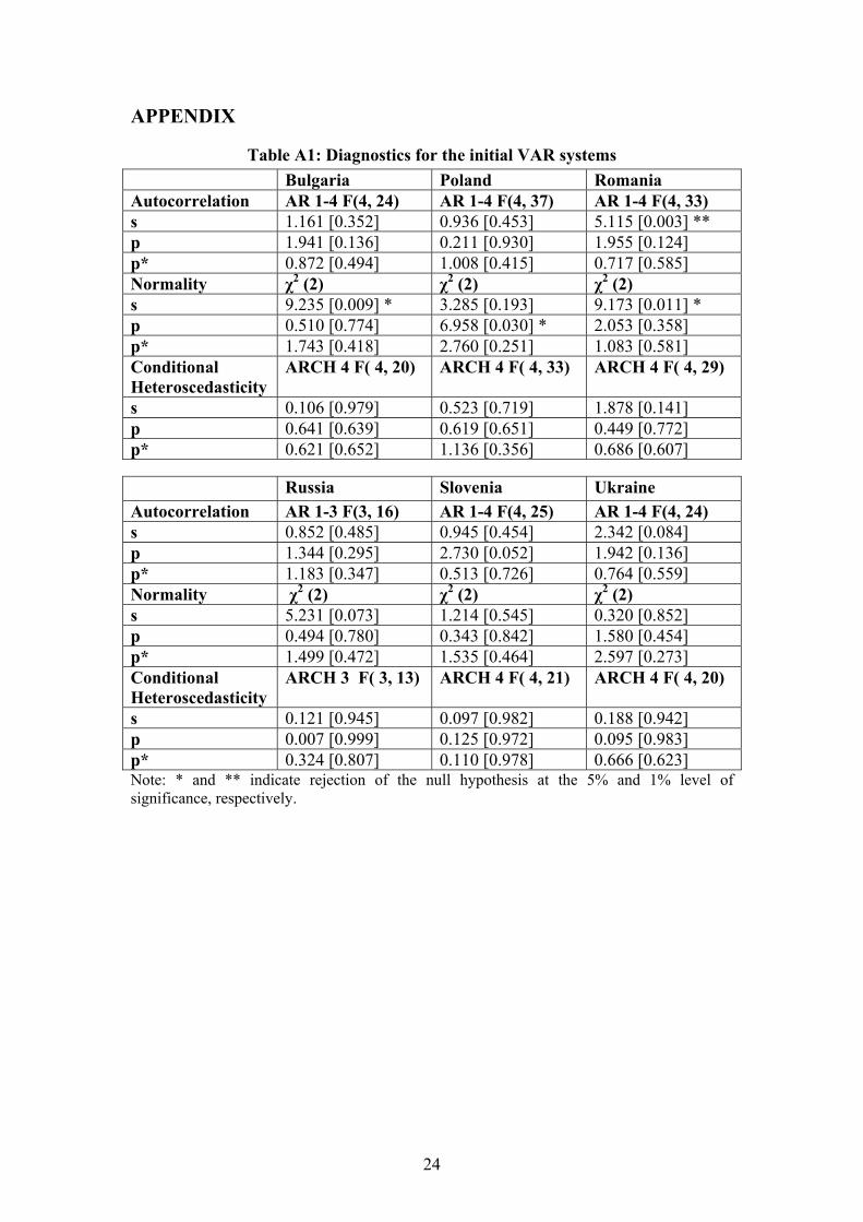
statistical properties of the residuals of the equations of the six systems are reported in

Table A1 in the Appendix. The diagnostics do not indicate any serious misspecification

and thus we can go on with the cointegration analysis.

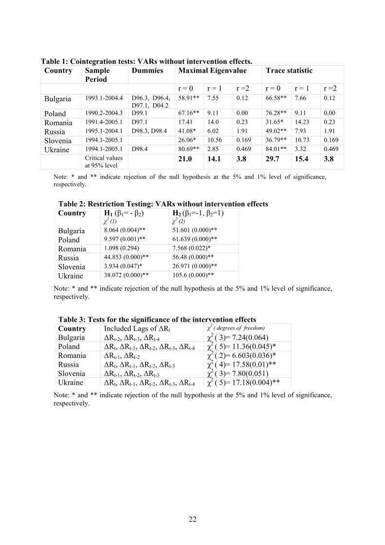
The results of the cointegration analysis are reported in Table 1. The second

column of Table 1 reports the estimation sample period, whereas the third column

names the dummies used. The outcomes of the maximum eigenvalue and trace

statistics are reported in columns 4 – 9. Computed trace statistics indicate that the null

hypothesis of non cointegration is rejected at the conventional 5% level of significance

for all countries. According to the maximum eigenvalue test outcomes, non-

cointegration is rejected at the 5% significance level for all economies except Romania,

for which rejection occurs at 10%. We thus proceed assuming that there exists one

cointegrating vector for all six systems. We then test for the validity of the theoretical

restrictions. The results are summarized in Table 2. According to the test statistics the

hypothesis of stationarity of the real exchange rate is rejected at the 5% significance

level in all countries in the sample. Weak PPP is rejected in all but the Romanian

system. The US-Romanian weak PPP relationship takes the form: s – 0.859 (p-p*).

5.3. The significance of the intervention effects

The second step in the empirical analysis is the evaluation of the importance of

the intervention effects on the short-run behavior of the exchange rates. To this end, we

include into the systems current and lagged values of ∆R. Four lagged levels for xt, a

constant, seasonal dummies and event specific dummies – the same as before – are

included in the systems. We initially included four lags for ∆R but then kept those

which were significant. As expected, current and lagged values of ∆R turn out to be

significant in the equations modelling the behaviour of the exchange rates and not in

the equations modelling domestic and foreign prices. The results are reported in Table

3. The second column reports the values of ∆R that are used in the six VARs. The third

column reports the respective χ2-statistics for the joint hypothesis that the reported

values of ∆R are not included in the equations modelling the behaviour of the exchange

rates. The hypothesis is rejected at the 5% significance level, for all but the Bulgarian

system, for which rejection occurs at 6.5%. We can thus state that the effects of ∆R

turn out to be significant for the short-run behaviour of the exchange rates in all

16

economies, finding which is consistent with the general consensus of the literature on

intervention.

5.4. Cointegration analysis with intervention effects

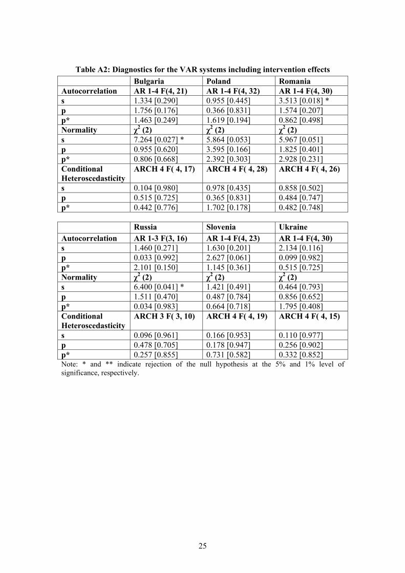
The inclusion of policy effects does not alter the stochastic properties of the

VAR systems as indicated by the results of the diagnostic tests, which are reported in

Table A2 in the Appendix. The findings of the Johansen technique for the six systems

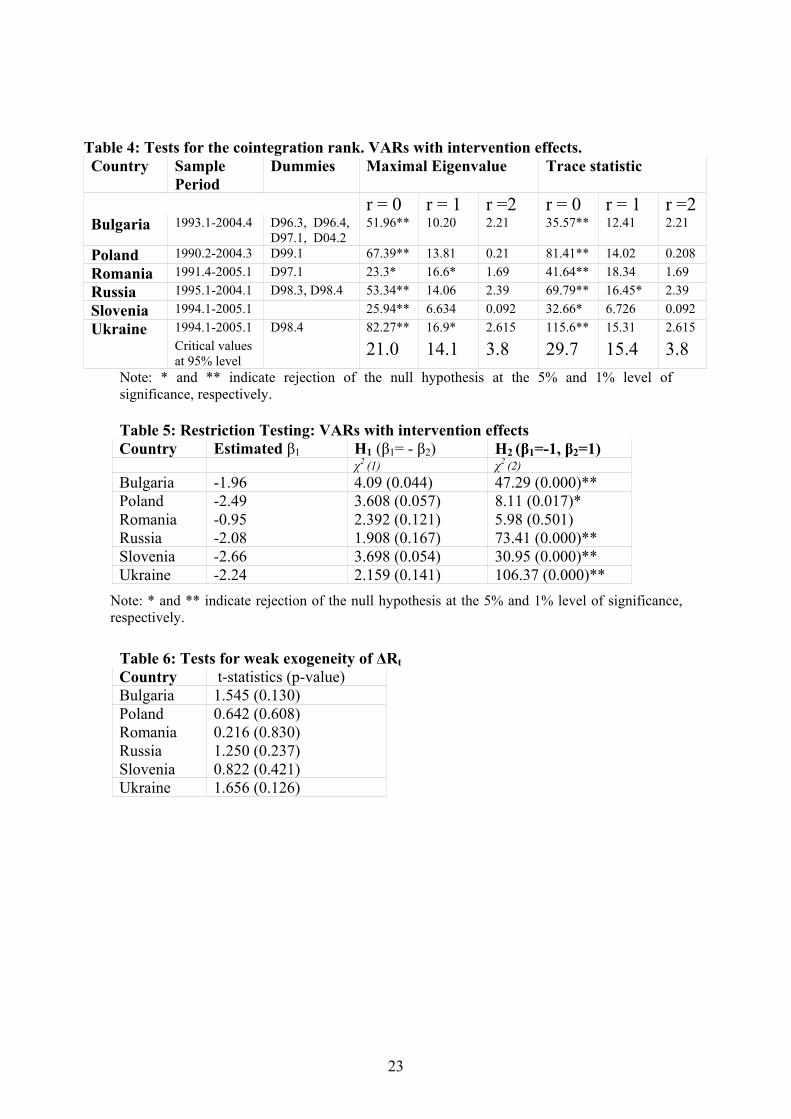
are presented in Table 4. As indicated by the results, the hypothesis that the

cointegration rank is zero is rejected at the 5% significance level by both likelihood

ratio tests, for all systems. We can thus assume one cointegrating vector for all six

cases.

Table 5 presents the outcomes of the test statistics for the theoretical

hypotheses concerning the specification of the cointegrating vectors. Columns 3 and 4

report the outcomes for the hypotheses of symmetry and proportionality, respectively.

Column 2 reports the values obtained for the magnitude of β1. According to the test

outcomes, now that policy effects are taken into account, weak PPP is accepted for all

six systems. All estimated β1s – excluding that for the Romanian system – take values

of high magnitude; they range from 1.96 in the case of Bulgaria to 2.66 in the case of

Slovenia. The high magnitudes of the β1s indicate that, in equilibrium, exchange rates

had to adjust significantly in order to accommodate the high rises in domestic prices

with respect to the foreign prices. This finding can be attributed to the fast

productivity growth observed in the CEEC economies during the examined period.

Differential productivity and growth rates resulted in stable real appreciations of the

CPI-based exchange rates for the five transition economies (see Coricelli and Jazbec,

2001, for similar arguments). The outcomes imply the presence of strong Balassa-

Samuelson effects which have operated for long periods of time. 17

It is only the estimated β1 coefficient in the Romanian relationship which takes

a value very close to unity (0.95). In fact, strong PPP is rejected in all but the

Romanian system. The rejection of strong PPP in the five countries can also be

17 The Balassa-Samuelson effect can be described briefly as follows: Suppose that the law of one price (LOOP) holds among traded goods. In the fast-growing economy, productivity growth, which is concentrated in the traded goods sector, will lead to wage rises without price rises. This rise in wages in the traded sector will lead to wage rises in the non-traded goods sector unjustified by productivity developments, and an overall rise in the CPI. Since LOOP holds in the traded goods sector and the nominal rate has remained constant, the real exchange rate appears appreciated.

17

attributed to Balassa-Samuelson effects. For the Romanian system, inclusion of

intervention effects, leads us to accept stationarity for the real exchange rate. This

implies that the central bank has been successful in the anti-inflationary policies they

pursued in the Romanian economy.

5.5. Weak exogeneity of ∆R with respect to the parameters of the long-run

relationships

The question of whether ∆R is weakly exogenous with respect to the estimated

parameters of the long-run relations of the six VARs also needs to be assessed. The

weak exogeneity test is essentially a test for the significance of the cointegrating

vector when used as an error correction term in a single equation, modelling the

behaviour of ∆R. The t-statistics for the error correction terms in the respective

equations modelling ∆R of the six economies are reported in Table 6. They all reject

statistical significance at the conventional 5% level. Thus, ∆R turns out to be weakly

exogenous for the cointegrating parameters of all six systems.

6. Conclusions

In the present paper we examine the effects of official intervention on: (i) the

short-run dynamics of the nominal exchange rates and (ii) the estimated long-run

behaviour of the real exchange rates (more precisely, the long-run behaviour of

nominal exchange rates in relation to the behaviour of relative prices). Our main

argument is that, by identifying and “isolating” the effects coming from intervention

operations on the short-run exchange rate dynamics (which can also be considered as

nominal shocks), we can then detect a long-run equilibrium relationship connecting

domestic and foreign prices and exchange rates, as formed by market forces alone.

The paper presents empirical findings for the validity of the above argument

by drawing on the experience of six CEEC economies in transition. These economies

seem ideal candidates to evaluate the above argument as they share a number of

common features: they all adopted flexible or managed floating exchange rate

regimes, whereas their monetary authorities intervened often in the foreign markets in

order to smooth exchange rate volatility or to pursue various monetary targets.

18

The results confirm our theoretical postulate: Effects due to authorities’

interventions in the foreign market turn out to be significant for the dynamic

behaviour of all nominal exchange rates under consideration. The results related to the

behaviour of exchange rates and relative prices in equilibrium change dramatically

once intervention effects are taken into account in the empirical modelling of the

short-run dynamics and indicate that omission of intervention effects would lead to

mistakenly rejecting a long-run exchange rate pattern based on PPP. In other words,

allowing for intervention effects, we indicate that PPP has enough content about the

behaviour of the real exchange rates in equilibrium. In addition, the estimated

equilibrium relationships indicate that the nominal exchange rates moved toward their

equilibrium values in a constant pattern, which nevertheless implied a constant

appreciation of the real exchange rates. This finding indicates the presence of strong

Balassa-Samuelson effects which have operated for long periods of time.

Nevertheless, stationarity of the real exchange rates is not accepted in five out of the

six economies, and this may also be due to productivity shocks and the impact that

productivity has on the pricing of the traded and non-traded goods and services

sectors.

19

References

Aguilar, J., Nydahl, S., 2000. Central bank intervention and exchange rates: the case of Sweden. Journal of International Financial Markets, Institutions and Money 10, 303-322.

Baillie, R.T., 2000. Central bank intervention. Journal of International Financial Markets, Institutions and Money 10, 225-228.

Brissimis, S.N., Chionis, D.P., 2004. Foreign exchange market intervention: implications of publicly announced and secret intervention for the euro exchange rate and its volatility. Journal of Policy Modeling 26, 661-673.

Brissimis, S.N., Sideris, D.A., Voumvaki, F.K., 2005. Testing long-run purchasing power parity under exchange rate targeting. Journal of International Money and Finance 24, 959-981.

Bonser-Neal, C., Tanner, G., 1996. Central bank intervention and the volatility of foreign exchange rates: evidence from the options market. Journal of International Money and Finance 15, 853-878.

Bonser-Neal, C., Roley, V.V, Sellon, G.H., 1998. Monetary policy actions, intervention, and exchange rates: a reexamination of the empirical relationships using federal funds rate target data. Journal of Business 71, 147-177.

Calvo, G.A., Reinhart, C.M., 2002. Fear of floating. The Quarterly Journal of Economics 117, 379-408.

Canales-Kriljenko, J.I., Guimaraes R., Karacadag, C., 2003. Official intervention in the foreign exchange market: elements of best practice. IMF Working Paper 03/152.

Christev, A., Noorbakhsh, A., 2000. Long-run purchasing power parity, prices and exchange rates in transition: the case of six Central and East European countries. Global Finance Journal 11, 87-108.

Choudhry, T., 1999. Purchasing power parity in high-inflation Eastern European countries: evidence from fractional and Harris-Inder cointegration tests. Journal of Macroeconomics 21, 293-308.

Clarida, R.H., Gali, J., 1994. Sources of real exchange rate fluctuations: how important are nominal shocks? Carnegie-Rochester Conference Series on Public Policy 41, 1-56.

Coricelli, F., Jazbec, B., 2001. Real exchange rate dynamics in transition economies. CEPR Discussion Paper 2869.

Dominguez, K., 1998. Central bank intervention and exchange rate volatility. Journal of International Money and Finance 17, 161-190.

Dominguez, K.M., Frankel, J.A., 1993a. Does Foreign Exchange Intervention Work? Institute for International Economics: Washington, D.C.

Dominguez, K.M., Frankel, J.A., 1993b. Foreign Exchange Intervention: An Empirical Assessment. In: Frankel, J.A. (Ed.), On Exchange Rates. MIT Press: Cambridge, Mass.

Edison, H., Cashin P.A., Liang, H., 2003. Foreign exchange intervention and the Australian dollar: has it mattered? IMF Working Paper 03/99.

20

Fatum R., Hutchison, M., 2003a. Is sterilised foreign exchange intervention effective after all? An event study approach. Economic Journal 113, 390-411.

Fatum R., Hutchison, M., 2003b. Effectiveness of official daily foreign exchange market intervention operations in Japan. NBER Working Paper 9648.

Frenkel, M., Pierdzioch, C., Stadtmann, G., 2005. The effects of Japanese foreign exchange market interventions on the yen/ U.S. dollar exchange rate volatility. International Review of Economics and Finance 14, 27-39.

Hagen, J., Zhou, J., 2002. The choice of exchange rate regimes: an empirical analysis for transition economies. CEPR Discussion Paper 3289.

Hung, J.H., 1997. Intervention strategies and exchange rate volatility: a noise trading perspective. Journal of International Money and Finance 16, 779-93.

Johansen, S., 1992. Cointegration in partial systems and the efficiency of single equation analysis. Journal of Econometrics 52, 389-402.

Johansen, S., 1995. Likelihood-Based Inference in Cointegrated Vector Autoregressive Models. Oxford University Press: Oxford.

Juselius, K., 1995. Do purchasing power parity and uncovered interest parity hold in the long run? An example of likelihood inference in a multivariate time-series model. Journal of Econometrics 69, 211-40.

Keller P.M., Richardson, T., 2003. Nominal anchors in the CIS. IMF Working Paper 03/179.

Kim, S., 2003. Monetary policy, foreign exchange intervention, and the exchange rate in a unifying framework. Journal of International Economics 60, 355-86

Kim, S.J., Kortian, T., Sheen, J., 2000. Central bank intervention and exchange rate volatility: Australian evidence. Journal of International Financial Markets, Institutions and Money 10, 381-405.

Neely, C. J., 2000. Are changes in foreign exchange reserves well correlated with official intervention? Federal Reserve Bank of St. Louis Review, September – October, 17-31.

Officer, L.H., 1976. The purchasing power parity theory of exchange rates: a review article. International Monetary Fund Staff Papers 23, 1-60.

Sarno, L., Taylor, M.P., 2002a. Official intervention in the foreign exchange market: is it effective, and, if so, how does it work? In: Sarno L., Taylor, M.P. (Eds.) The Economics of Exchange Rates. Cambridge University Press: Cambridge, UK.

Sarno, L., Taylor, M.P, 2002b. Purchasing power parity and the real exchange rate. IMF Staff Papers 49, 65-105.

Sideris, D., 2006. Purchasing power parity in economies in transition: evidence from Central and East European countries. Applied Financial Economics 16, 135-143.

Sweeney, R.J., 1999. Intervention strategy and purchasing power parity. In: Sweeney, R.J., Wihlborg, C.G., Willett, T.D. (Eds.), Exchange-Rate Policies for Emerging Market Economies. Westview Press: Boulder and Oxford.

Szakmary, A.C., Mathur, I., 1997.Central bank intervention and trading rule profits in foreign exchange markets. Journal of International Money and Finance 16, 513-535.

21

Taylor, D., 1982. Official intervention in the foreign exchange market. Journal of Political Economy 90, 356-68.

Taylor, M.P., 2004. Is official exchange rate intervention effective? Economica 71, 1-12.

Thacker, N., 1995. Does PPP hold in the transition economies? The case of Poland and Hungary. Applied Economics 27, 477-481.

Usman, A.A., Savides, A., 1994. Foreign exchange market intervention and the French franc Deutschemark exchange rate. Journal of International Financial Markets, Institutions and Money 4, 49-60.

22

Table 1: Cointegration tests: VARs without intervention effects. Country Sample

Period Dummies Maximal Eigenvalue Trace statistic

r = 0 r = 1 r =2 r = 0 r = 1 r =2 Bulgaria 1993.1-2004.4 D96.3, D96.4,

D97.1, D04.2 58.91** 7.55 0.12 66.58** 7.66 0.12

Poland 1990.2-2004.3 D99.1 67.16** 9.11 0.00 76.28** 9.11 0.00 Romania 1991.4-2005.1 D97.1 17.41 14.0 0.23 31.65* 14.23 0.23 Russia 1995.1-2004.1 D98.3, D98.4 41.08* 6.02 1.91 49.02** 7.93 1.91 Slovenia 1994.1-2005.1 26.06* 10.56 0.169 36.79** 10.73 0.169 Ukraine 1994.1-2005.1 D98.4 80.69** 2.85 0.469 84.01** 3.32 0.469

Critical values at 95% level

21.0 14.1 3.8 29.7 15.4 3.8

Note: * and ** indicate rejection of the null hypothesis at the 5% and 1% level of significance, respectively.

Table 2: Restriction Testing: VARs without intervention effects Country H1 (β1= - β2) H2 (β1=-1, β2=1) χ2 (1) χ2 (2)

Bulgaria 8.064 (0.004)** 51.601 (0.000)** Poland 9.597 (0.001)** 61.639 (0.000)** Romania 1.098 (0.294) 7.568 (0.022)* Russia 44.853 (0.000)** 56.48 (0.000)** Slovenia 3.934 (0.047)* 26.971 (0.000)** Ukraine 38.072 (0.000)** 105.6 (0.000)**

Note: * and ** indicate rejection of the null hypothesis at the 5% and 1% level of significance, respectively.

Table 3: Tests for the significance of the intervention effects Country Included Lags of ∆Rt χ2 ( degrees of freedom)

Bulgaria ∆Rt-2, ∆Rt-3, ∆Rt-4 χ2 ( 3)= 7.24(0.064) Poland ∆Rt, ∆Rt-1, ∆Rt-2, ∆Rt-3, ∆Rt-4 χ2 ( 5)= 11.36(0.045)* Romania ∆Rt-1, ∆Rt-2 χ2 ( 2)= 6.603(0.036)* Russia ∆Rt, ∆Rt-1, ∆Rt-2, ∆Rt-3 χ2 ( 4)= 17.58(0.01)** Slovenia ∆Rt-1, ∆Rt-2, ∆Rt-3 χ2 ( 3)= 7.80(0.051) Ukraine ∆Rt, ∆Rt-1, ∆Rt-2, ∆Rt-3, ∆Rt-4 χ2 ( 5)= 17.18(0.004)**

Note: * and ** indicate rejection of the null hypothesis at the 5% and 1% level of significance, respectively.

23

Table 4: Tests for the cointegration rank. VARs with intervention effects. Country Sample

Period Dummies Maximal Eigenvalue Trace statistic

r = 0 r = 1 r =2 r = 0 r = 1 r =2 Bulgaria 1993.1-2004.4 D96.3, D96.4,

D97.1, D04.2 51.96** 10.20 2.21 35.57** 12.41 2.21

Poland 1990.2-2004.3 D99.1 67.39** 13.81 0.21 81.41** 14.02 0.208 Romania 1991.4-2005.1 D97.1 23.3* 16.6* 1.69 41.64** 18.34 1.69 Russia 1995.1-2004.1 D98.3, D98.4 53.34** 14.06 2.39 69.79** 16.45* 2.39 Slovenia 1994.1-2005.1 25.94** 6.634 0.092 32.66* 6.726 0.092 Ukraine 1994.1-2005.1 D98.4 82.27** 16.9* 2.615 115.6** 15.31 2.615 Critical values

at 95% level 21.0 14.1 3.8 29.7 15.4 3.8

Note: * and ** indicate rejection of the null hypothesis at the 5% and 1% level of significance, respectively. Table 5: Restriction Testing: VARs with intervention effects Country Estimated β1 H1 (β1= - β2) H2 (β1=-1, β2=1) χ2 (1) χ2 (2) Bulgaria -1.96 4.09 (0.044) 47.29 (0.000)** Poland -2.49 3.608 (0.057) 8.11 (0.017)* Romania -0.95 2.392 (0.121) 5.98 (0.501) Russia -2.08 1.908 (0.167) 73.41 (0.000)** Slovenia -2.66 3.698 (0.054) 30.95 (0.000)** Ukraine -2.24 2.159 (0.141) 106.37 (0.000)**

Note: * and ** indicate rejection of the null hypothesis at the 5% and 1% level of significance, respectively.

Table 6: Tests for weak exogeneity of ∆Rt Country t-statistics (p-value) Bulgaria 1.545 (0.130) Poland 0.642 (0.608) Romania 0.216 (0.830) Russia 1.250 (0.237) Slovenia 0.822 (0.421) Ukraine 1.656 (0.126)

24

APPENDIX

Table A1: Diagnostics for the initial VAR systems Bulgaria Poland Romania Autocorrelation AR 1-4 F(4, 24) AR 1-4 F(4, 37) AR 1-4 F(4, 33) s 1.161 [0.352] 0.936 [0.453] 5.115 [0.003] ** p 1.941 [0.136] 0.211 [0.930] 1.955 [0.124] p* 0.872 [0.494] 1.008 [0.415] 0.717 [0.585] Normality χ2 (2) χ2 (2) χ2 (2) s 9.235 [0.009] * 3.285 [0.193] 9.173 [0.011] * p 0.510 [0.774] 6.958 [0.030] * 2.053 [0.358] p* 1.743 [0.418] 2.760 [0.251] 1.083 [0.581] Conditional Heteroscedasticity

ARCH 4 F( 4, 20) ARCH 4 F( 4, 33) ARCH 4 F( 4, 29)

s 0.106 [0.979] 0.523 [0.719] 1.878 [0.141] p 0.641 [0.639] 0.619 [0.651] 0.449 [0.772] p* 0.621 [0.652] 1.136 [0.356] 0.686 [0.607]

Russia Slovenia Ukraine Autocorrelation AR 1-3 F(3, 16) AR 1-4 F(4, 25) AR 1-4 F(4, 24) s 0.852 [0.485] 0.945 [0.454] 2.342 [0.084] p 1.344 [0.295] 2.730 [0.052] 1.942 [0.136] p* 1.183 [0.347] 0.513 [0.726] 0.764 [0.559] Normality χ2 (2) χ2 (2) χ2 (2) s 5.231 [0.073] 1.214 [0.545] 0.320 [0.852] p 0.494 [0.780] 0.343 [0.842] 1.580 [0.454] p* 1.499 [0.472] 1.535 [0.464] 2.597 [0.273] Conditional Heteroscedasticity

ARCH 3 F( 3, 13) ARCH 4 F( 4, 21) ARCH 4 F( 4, 20)

s 0.121 [0.945] 0.097 [0.982] 0.188 [0.942] p 0.007 [0.999] 0.125 [0.972] 0.095 [0.983] p* 0.324 [0.807] 0.110 [0.978] 0.666 [0.623] Note: * and ** indicate rejection of the null hypothesis at the 5% and 1% level of significance, respectively.

25

Table A2: Diagnostics for the VAR systems including intervention effects Bulgaria Poland Romania Autocorrelation AR 1-4 F(4, 21) AR 1-4 F(4, 32) AR 1-4 F(4, 30) s 1.334 [0.290] 0.955 [0.445] 3.513 [0.018] * p 1.756 [0.176] 0.366 [0.831] 1.574 [0.207] p* 1.463 [0.249] 1.619 [0.194] 0.862 [0.498] Normality χ2 (2) χ2 (2) χ2 (2) s 7.264 [0.027] * 5.864 [0.053] 5.967 [0.051] p 0.955 [0.620] 3.595 [0.166] 1.825 [0.401] p* 0.806 [0.668] 2.392 [0.303] 2.928 [0.231] Conditional Heteroscedasticity

ARCH 4 F( 4, 17) ARCH 4 F( 4, 28) ARCH 4 F( 4, 26)

s 0.104 [0.980] 0.978 [0.435] 0.858 [0.502] p 0.515 [0.725] 0.365 [0.831] 0.484 [0.747] p* 0.442 [0.776] 1.702 [0.178] 0.482 [0.748] Russia Slovenia Ukraine Autocorrelation AR 1-3 F(3, 16) AR 1-4 F(4, 23) AR 1-4 F(4, 30) s 1.460 [0.271] 1.630 [0.201] 2.134 [0.116] p 0.033 [0.992] 2.627 [0.061] 0.099 [0.982] p* 2.101 [0.150] 1.145 [0.361] 0.515 [0.725] Normality χ2 (2) χ2 (2) χ2 (2) s 6.400 [0.041] * 1.421 [0.491] 0.464 [0.793] p 1.511 [0.470] 0.487 [0.784] 0.856 [0.652] p* 0.034 [0.983] 0.664 [0.718] 1.795 [0.408] Conditional Heteroscedasticity

ARCH 3 F( 3, 10) ARCH 4 F( 4, 19) ARCH 4 F( 4, 15)

s 0.096 [0.961] 0.166 [0.953] 0.110 [0.977] p 0.478 [0.705] 0.178 [0.947] 0.256 [0.902] p* 0.257 [0.855] 0.731 [0.582] 0.332 [0.852] Note: * and ** indicate rejection of the null hypothesis at the 5% and 1% level of significance, respectively.

26

27

BANK OF GREECE WORKING PAPERS 31. Hall, S. G. and G. Hondroyiannis, “Measuring the Correlation of Shocks between

the EU-15 and the New Member Countries”, January 2006. 32. Christodoulakis, G. A. and S. E. Satchell, “Exact Elliptical Distributions for

Models of Conditionally Random Financial Volatility”, January 2006. 33. Gibson, H. D., N. T. Tsaveas and T. Vlassopoulos, “Capital Flows, Capital

Account Liberalisation and the Mediterranean Countries”, February 2006. 34. Tavlas, G. S. and P. A. V. B. Swamy, “The New Keynesian Phillips Curve and

Inflation Expectations: Re-specification and Interpretation”, March 2006. 35. Brissimis, S. N. and N. S. Magginas, “Monetary Policy Rules under

Heterogeneous Inflation Expectations”, March 2006. 36. Kalfaoglou, F. and A. Sarris, “Modeling the Components of Market Discipline”,

April 2006. 37. Kapopoulos, P. and S. Lazaretou, “Corporate Ownership Structure and Firm

Performance: Evidence from Greek Firms”, April 2006. 38. Brissimis, S. N. and N. S. Magginas, “Inflation Forecasts and the New Keynesian

Phillips Curve”, May 2006. 39. Issing, O., “Europe’s Hard Fix: The Euro Area”, including comments by Mario I.

Blejer and Leslie Lipschitz, May 2006. 40. Arndt, S. W., “Regional Currency Arrangements in North America”, including

comments by Steve Kamin and Pierre L. Siklos, May 2006. 41. Genberg, H., “Exchange-Rate Arrangements and Financial Integration in East

Asia: On a Collision Course?”, including comments by James A. Dorn and Eiji Ogawa, May 2006.

42. Christl, J., “Regional Currency Arrangements: Insights from Europe”, including

comments by Lars Jonung and the concluding remarks and main findings of the workshop by Eduard Hochreiter and George Tavlas, June 2006.

43. Edwards, S., “Monetary Unions, External Shocks and Economic Performance: A

Latin American Perspective”, including comments by Enrique Alberola, June 2006.

44. Cooper, R. N., “Proposal for a Common Currency Among Rich Democracies”

and Bordo, M. and H. James, “One World Money, Then and Now”, including comments by Sergio L. Schmukler, June 2006.

45. Williamson, J., “A Worldwide System of Reference Rates”, including comments

by Marc Flandreau, August 2006.

28

46. Brissimis, S. N., M. D. Delis and E. G. Tsionas, “Technical and Allocative

Efficiency in European Banking”, September 2006. 47. Athanasoglou, P. P., M. D. Delis and C. K. Staikouras, “Determinants of Bank

Profitability in the South Eastern European Region”, September 2006. 48. Petroulas, P., “The Effect of the Euro on Foreign Direct Investment”, October

2006. 49. Andreou, A. S. and G. A. Zombanakis, “Computational Intelligence in Exchange-

Rate Forecasting”, November 2006. 50. Milionis, A. E., “An Alternative Definition of Market Efficiency and Some

Comments on its Empirical Testing”, November 2006. 51. Brissimis, S. N. and T. S. Kosma, “Market Conduct, Price Interdependence and

Exchange Rate Pass-Through”, December 2006. 52. Anastasatos, T. G. and I. R. Davidson, “How Homogenous are Currency Crises?

A Panel Study Using Multiple Response Models”, December, 2006. 53. Angelopoulou, E. and H. D. Gibson, “The Balance Sheet Channel of Monetary

Policy Transmission: Evidence from the UK”, January, 2007. 54. Brissimis, S. N. and M. D. Delis, “Identification of a Loan Supply Function: A

Cross-Country Test for the Existence of a Bank Lending Channel”, January, 2007.

55. Angelopoulou, E., “The Narrative Approach for the Identification of Monetary

Policy Shocks in a Small Open Economy”, February, 2007.