ASC Report No. 31/2015

E�cient numerical computation

of direct exchange areas

in thermal radiation analysis

M. Feischl, T. Führer, M. Niederer, S. Strommer, A.

Steinboeck, and D. Praetorius

Institute for Analysis and Scienti�c Computing �

Vienna University of Technology � TU Wien

www.asc.tuwien.ac.at ISBN 978-3-902627-05-6

Most recent ASC Reports

30/2015 B. Düring, P. Fuchs, and A. Jüngel

A higher-order gradient �ow schemefor a singular one-dimensionaldi�usion equation

29/2015 C. Erath and D. Praetorius

Adaptive �nite volume methods with convergence rates

28/2015 W. Auzinger, O. Koch, M. Schöbinger, E. Weinmüller

A new version of the code bvpsuite for singular BVPs in ODEs: Nonlinear solverand its application to m-Laplacians.

27/2015 C. Lehrenfeld, J. Schöberl

High order exactly divergence-free Hybrid Discontinuous Galerkin Methods forunsteady incompressible �ows

26/2015 A. Jüngel, and S. Schuchnigg

Entropy-dissipating semi-discrete Runge-Kutta schemes for nonlinear di�usionequations

25/2015 W. Auzinger, H. Hofstätter, D. Ketcheson, O. Koch

Practical splitting methods for the adaptive integration of nonlinear evolutionequations.Part I: Construction of optimized schemes and pairs of schemes

24/2015 J. Burkotová, M. Hubner, I. Rachunková, and E.B. Weinmüller

Asymptotic properties of Kneser solutions to nonlinear second order ODEs withregularly varying coe�cients

23/2015 C. Abert, G. Hrkac, D. Praetorius, M. Ruggeri, D. Suess

Coupling of dynamical micromagnetism and a stationary spin drift-di�usionequation: A step towards a fully implicit spintronics frame

22/2015 F. Achleitner, A. Arnold and D. Stürzer

Large-time behavior in non-symmetric Fokker-Planck equations

21/2015 J. Burkotová, I. Rachunková, and E.B. Weinmüller

On singular BVPs with unsmooth data.Part 2: Converegence of the collocation schemes

Institute for Analysis and Scienti�c ComputingVienna University of TechnologyWiedner Hauptstraÿe 8�101040 Wien, Austria

E-Mail: admin@asc.tuwien.ac.at

WWW: http://www.asc.tuwien.ac.at

FAX: +43-1-58801-10196

ISBN 978-3-902627-05-6

c© Alle Rechte vorbehalten. Nachdruck nur mit Genehmigung des Autors.

ASCTU WIEN

EFFICIENT NUMERICAL COMPUTATION OF DIRECT

EXCHANGE AREAS IN THERMAL RADIATION ANALYSIS

Abbreviated title: EFFICIENT COMPUTATION OF DIRECT EXCHANGE AREAS

M. Feischla, T. Fuhrera, M. Niedererb, S. Strommerb, A. Steinboeckb,∗, and D. Praetoriusa

aInstitute of Analysis and Scientific Computing, Vienna University of Technology,

Wiedner Hauptstraße 8, 1040 Vienna, AustriabAutomation and Control Institute, Vienna University of Technology,

Gußhausstraße 27–29, 1040 Vienna, Austria

(Received 00 Month 20XX; final version received 00 Month 20XX)

Abstract: The analysis of thermal radiation in multi-surface enclosures typically involvesmultiple integrals with four, five, or six variables. Major difficulties for the numerical evalu-ation of these integrals are non-convex geometries and singular integral kernels. This paperpresents hierarchical visibility concepts and coordinate transformations which eliminate thesedifficulties. In the transformed form, standard quadrature techniques are applied and accurateresults are achieved with moderate numerical effort. In benchmark example problems, theeffectiveness and accuracy of the method are validated. A simulation model of an industrialfurnace demonstrates the applicability of the method for large-scale problems.

NOMENCLATURE

α tupleBα bounding boxb radiosity, W/m2

C(α) function for computing the visibilityD integration domaind side length, m2

ε emissivityf continuous function or part of the kernel k, m4

g part of the integral kernel k, 1/m2

H heat flux density absorbed by a volume zone, W/m2

θ incident or emergent angle, radh irradiance, W/m2

I total intensity, W/(m2sr)Λ coordinate transformationK absorption coefficient, 1/mk integral kernel, 1/m4

M order of quadratureNS number of surface zonesNV number of volume zones

∗Corresponding author. Email: andreas.steinboeck@tuwien.ac.atSeptember 07, 2015

1

Q net heat flow into volume zone, Wq net heat flow into surface zone, Wσ Stefan-Boltzmann constant, W/(m2K4)r distance coordinate along a ray, mrj , rij geometrical length of a ray, mrij optical length of a raySα set of barycenters of surfaces zonesS(α) functions for generating a hierarchy of bounding boxesS surface zone, m2

s evaluation point of Gaussian quadraturesisj surface-surface direct exchange area, m2

sivj surface-volume direct exchange area, m2

T gas temperature, Kt surface temperature, KΦ function for a transformation of integration domainsV volume zone, m3

Vref reference volume zonevisj volume-surface direct exchange area, m2

vivj volume-volume direct exchange area, m2

W integration domainw weight of Gaussian quadrature

Coordinates

~α, ~β normalized coordinates in reference volume zone~x coordinates in volume zone~γ relative coordinates

Subscripts

i, j index of zone or index valuek, n index value

1. INTRODUCTION

Heat transfer by gray thermal radiation in enclosures formed by diffuse surfaces and filledwith participating gas can be efficiently analyzed by means of the zone method [1]. Insteadof a rigorous solution of the multiple integrals that emerge from the direct application ofthe radiative transfer equation [2, 3], the zone method uses a spatial discretization of theradiation geometry to obtain a finite-dimensional linear relation between the radiativeheat flows and the fourth powers of the temperatures. The discretization is found by di-viding the calculation domain into isothermal surface and volume sections. The approachmay be considered as a numerical quadrature method that facilitates a direct geometricinterpretation.The zone method, which was originally suggested by Hottel and coworkers [1, 4], is

described in detail in [2, 3]. Section 1.1 of this paper provides a concise overview ofthis method. Reviews of various other modeling methods for radiative heat transfer arereported in [5, 6, 7, 8, 9, 10, 11].According to [8], the zone method is one of the fastest approaches for analyzing thermal

radiation if the exchange areas are known. However, the calculation of direct exchangeareas is still a time-consuming and thus limiting factor of the zone method. In fact, it

2

involves integrals with four, five, or six variables [2, 3]. Currently, there is no perspectiveto compute direct exchange areas in real time. Despite growing computer power and theadvent of multi-core systems and parallel computing, the computation of direct exchangeareas for general three-dimensional problems with complex geometries is still not feasi-ble within reasonable times. This conclusion may also be drawn from the literature inthis field, which is briefly reviewed in Section 1.2. The lack of an efficient method forcalculating direct exchange areas is the principal impetus for this work.The paper is organized as follows: Section 2 demonstrates that the multiple integrals

associated with direct exchange areas should not be solved by direct application of numer-ical quadrature techniques due to singularity problems. Therefore, we explore in Section3 how coordinate and geometric transformations can avoid these singularities. In Section4, we validated the effectiveness and accuracy of the method based on benchmark exam-ple problems. In a case study, we use the approach in a simulation model of an industrialfurnace and compare the simulation results with measurements from the real plant. Thisdemonstrates the applicability of the method to large-scale problems.

1.1. Zone Method

Consider a volume that is filled with participating gas. In this volume, let the straightpath of a single ray of thermal radiation be parameterized by the distance coordinater. The total intensity of the ray at some point r is I(r). From the radiative transferequation [2, 3], it is known that the total intensity of the ray is attenuated according to

I(rj) = I(ri)e−rij (1)

as it travels from r = ri to r = rj through the participating gas. The dimensionlessquantity

rij =

∫ rj

ri

K(r)dr (2)

with the absorption coefficient K(r) is also known as optical thickness of the path fromri to rj . In a gaseous medium where K is constant, K−1 is the mean free path of aphoton until it is absorbed. In Eq. (1), we have not considered that the total intensitymay also increase because of radiative emission of the gas itself. This effect is capturedby the term

K(r)σ

πT 4dV , (3)

which is the total heat flux emitted by an infinitesimal volume element dV per unit solidangle. T is the local gas temperature and σ is the Stefan-Boltzmann constant. The termσT 4/π represents the total intensity of black bodies.

dS, t, ε

θ

Figure 1. Emergent angle of an emitting surface.

An infinitesimal section dS of a solid, gray, diffuse surface with the temperature t emits

3

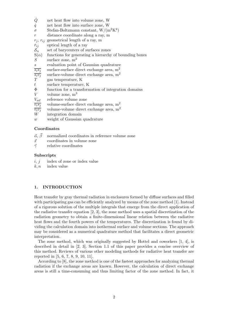
the directional total heat flux

εσ

πt4 cos(θ)dS (4)

per unit solid angle. The radiative heat flux depends on the emergent angle θ ∈ [0, π/2](cf. Fig. 1) insofar as it is proportional to the projected area cos(θ)dS of the emitter.Moreover, it is proportional to the emissivity ε ∈ [0, 1], which is a surface property.

S1 S2

Sj , tj

Sn

qj

Vi,Ti

V1

V2VN

Qi

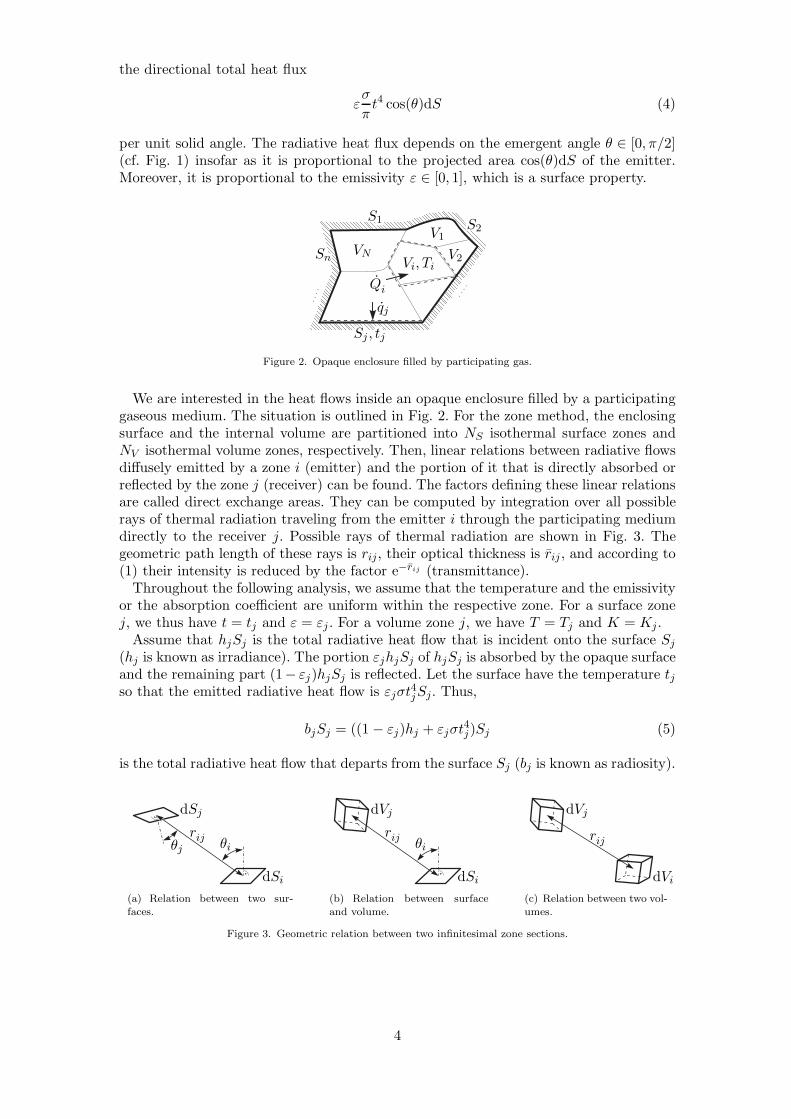
Figure 2. Opaque enclosure filled by participating gas.

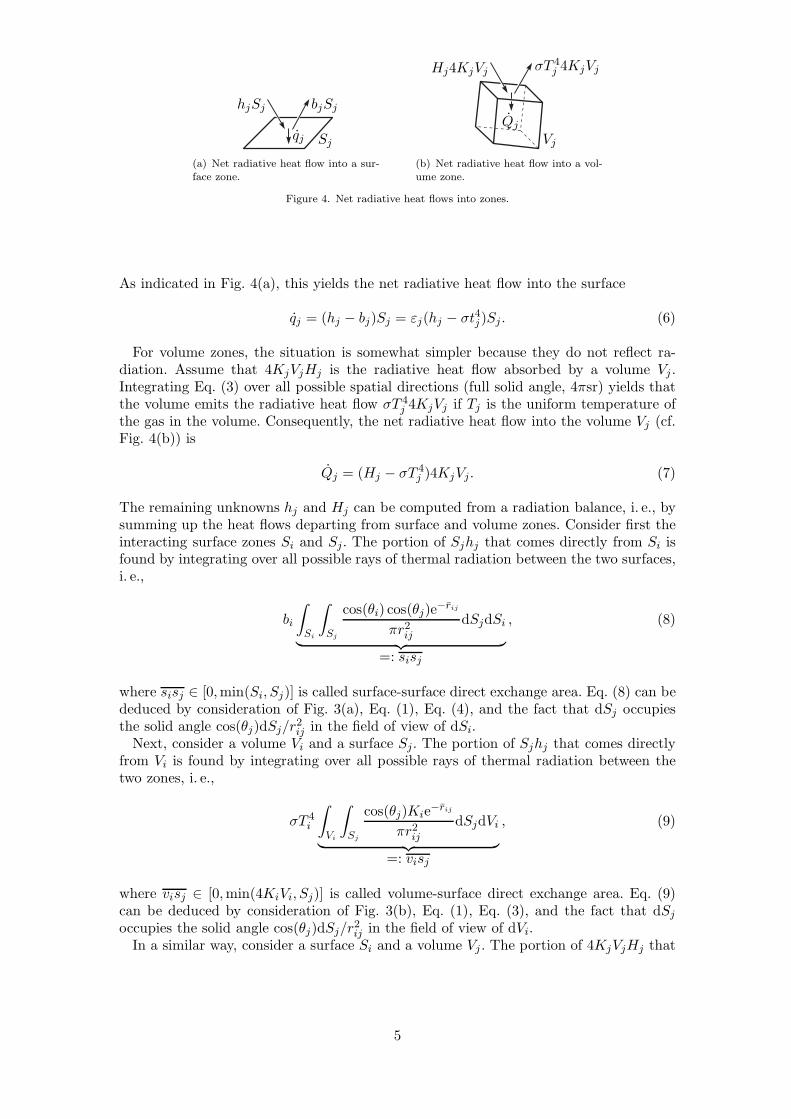
We are interested in the heat flows inside an opaque enclosure filled by a participatinggaseous medium. The situation is outlined in Fig. 2. For the zone method, the enclosingsurface and the internal volume are partitioned into NS isothermal surface zones andNV isothermal volume zones, respectively. Then, linear relations between radiative flowsdiffusely emitted by a zone i (emitter) and the portion of it that is directly absorbed orreflected by the zone j (receiver) can be found. The factors defining these linear relationsare called direct exchange areas. They can be computed by integration over all possiblerays of thermal radiation traveling from the emitter i through the participating mediumdirectly to the receiver j. Possible rays of thermal radiation are shown in Fig. 3. Thegeometric path length of these rays is rij, their optical thickness is rij , and according to(1) their intensity is reduced by the factor e−rij (transmittance).Throughout the following analysis, we assume that the temperature and the emissivity

or the absorption coefficient are uniform within the respective zone. For a surface zonej, we thus have t = tj and ε = εj . For a volume zone j, we have T = Tj and K = Kj.Assume that hjSj is the total radiative heat flow that is incident onto the surface Sj

(hj is known as irradiance). The portion εjhjSj of hjSj is absorbed by the opaque surfaceand the remaining part (1− εj)hjSj is reflected. Let the surface have the temperature tjso that the emitted radiative heat flow is εjσt

4jSj. Thus,

bjSj = ((1 − εj)hj + εjσt4j)Sj (5)

is the total radiative heat flow that departs from the surface Sj (bj is known as radiosity).

dSi

dSj

rijθiθj

(a) Relation between two sur-faces.

dSi

rijθi

dVj

(b) Relation between surfaceand volume.

rij

dVj

dVi

(c) Relation between two vol-umes.

Figure 3. Geometric relation between two infinitesimal zone sections.

4

Sj

hjSj bjSj

qj

(a) Net radiative heat flow into a sur-face zone.

Vj

Hj4KjVj σT 4j 4KjVj

Qj

(b) Net radiative heat flow into a vol-ume zone.

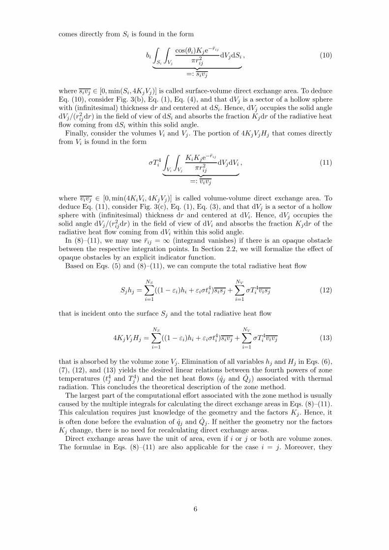
Figure 4. Net radiative heat flows into zones.

As indicated in Fig. 4(a), this yields the net radiative heat flow into the surface

qj = (hj − bj)Sj = εj(hj − σt4j)Sj . (6)

For volume zones, the situation is somewhat simpler because they do not reflect ra-diation. Assume that 4KjVjHj is the radiative heat flow absorbed by a volume Vj .Integrating Eq. (3) over all possible spatial directions (full solid angle, 4πsr) yields thatthe volume emits the radiative heat flow σT 4

j 4KjVj if Tj is the uniform temperature ofthe gas in the volume. Consequently, the net radiative heat flow into the volume Vj (cf.Fig. 4(b)) is

Qj = (Hj − σT 4j )4KjVj. (7)

The remaining unknowns hj and Hj can be computed from a radiation balance, i. e., bysumming up the heat flows departing from surface and volume zones. Consider first theinteracting surface zones Si and Sj. The portion of Sjhj that comes directly from Si isfound by integrating over all possible rays of thermal radiation between the two surfaces,i. e.,

bi

∫

Si

∫

Sj

cos(θi) cos(θj)e−rij

πr2ijdSjdSi

︸ ︷︷ ︸=: sisj

, (8)

where sisj ∈ [0,min(Si, Sj)] is called surface-surface direct exchange area. Eq. (8) can bededuced by consideration of Fig. 3(a), Eq. (1), Eq. (4), and the fact that dSj occupiesthe solid angle cos(θj)dSj/r

2ij in the field of view of dSi.

Next, consider a volume Vi and a surface Sj. The portion of Sjhj that comes directlyfrom Vi is found by integrating over all possible rays of thermal radiation between thetwo zones, i. e.,

σT 4i

∫

Vi

∫

Sj

cos(θj)Kie−rij

πr2ijdSjdVi

︸ ︷︷ ︸=: visj

, (9)

where visj ∈ [0,min(4KiVi, Sj)] is called volume-surface direct exchange area. Eq. (9)can be deduced by consideration of Fig. 3(b), Eq. (1), Eq. (3), and the fact that dSj

occupies the solid angle cos(θj)dSj/r2ij in the field of view of dVi.

In a similar way, consider a surface Si and a volume Vj . The portion of 4KjVjHj that

5

comes directly from Si is found in the form

bi

∫

Si

∫

Vj

cos(θi)Kje−rij

πr2ijdVjdSi

︸ ︷︷ ︸=: sivj

, (10)

where sivj ∈ [0,min(Si, 4KjVj)] is called surface-volume direct exchange area. To deduceEq. (10), consider Fig. 3(b), Eq. (1), Eq. (4), and that dVj is a sector of a hollow spherewith (infinitesimal) thickness dr and centered at dSi. Hence, dVj occupies the solid angledVj/(r

2ijdr) in the field of view of dSi and absorbs the fraction Kjdr of the radiative heat

flow coming from dSi within this solid angle.Finally, consider the volumes Vi and Vj . The portion of 4KjVjHj that comes directly

from Vi is found in the form

σT 4i

∫

Vi

∫

Vj

KiKje−rij

πr2ijdVjdVi

︸ ︷︷ ︸=: vivj

, (11)

where vivj ∈ [0,min(4KiVi, 4KjVj)] is called volume-volume direct exchange area. Todeduce Eq. (11), consider Fig. 3(c), Eq. (1), Eq. (3), and that dVj is a sector of a hollowsphere with (infinitesimal) thickness dr and centered at dVi. Hence, dVj occupies thesolid angle dVj/(r

2ijdr) in the field of view of dVi and absorbs the fraction Kjdr of the

radiative heat flow coming from dVi within this solid angle.In (8)–(11), we may use rij = ∞ (integrand vanishes) if there is an opaque obstacle

between the respective integration points. In Section 2.2, we will formalize the effect ofopaque obstacles by an explicit indicator function.Based on Eqs. (5) and (8)–(11), we can compute the total radiative heat flow

Sjhj =

NS∑

i=1

((1− εi)hi + εiσt4i )sisj +

NV∑

i=1

σT 4i visj (12)

that is incident onto the surface Sj and the total radiative heat flow

4KjVjHj =

NS∑

i=1

((1− εi)hi + εiσt4i )sivj +

NV∑

i=1

σT 4i vivj (13)

that is absorbed by the volume zone Vj. Elimination of all variables hj andHj in Eqs. (6),(7), (12), and (13) yields the desired linear relations between the fourth powers of zonetemperatures (t4j and T 4

j ) and the net heat flows (qj and Qj) associated with thermalradiation. This concludes the theoretical description of the zone method.The largest part of the computational effort associated with the zone method is usually

caused by the multiple integrals for calculating the direct exchange areas in Eqs. (8)–(11).This calculation requires just knowledge of the geometry and the factors Kj. Hence, it

is often done before the evaluation of qj and Qj. If neither the geometry nor the factorsKj change, there is no need for recalculating direct exchange areas.Direct exchange areas have the unit of area, even if i or j or both are volume zones.

The formulae in Eqs. (8)–(11) are also applicable for the case i = j. Moreover, they

6

satisfy the reciprocity relations

sisj = sjsi (14a)

visj = sjvi (14b)

vivj = vjvi (14c)

and the summation rules

Sj =

NS∑

i=1

sisj +

NV∑

i=1

visj (15a)

4KjVj =

NS∑

i=1

sivj +

NV∑

i=1

vivj (15b)

(cf. [2, 3, 10]). These relations can be helpful for validating numerical results of directexchange areas or for reducing the workload when computing them. When solving themultiple integrals in Eqs. (8)–(11), a considerable difficulty is the singularity associatedwith rij → 0. This will be further analyzed in Section 2.

1.2. Existing Approaches for Explicit Calculation of Direct Exchange

Areas

Numerical values for direct exchange areas in rectangular geometries are given in theform of charts in [12]. Moreover, curve fitting techniques are applied to obtain exponentialfunctions that approximate the given numerical results [10].In Cartesian coordinates, the length rij of a ray ~rij = ~xj − ~xi emitted from ~xi to ~xj is

computed by

rij := |~xi − ~xj | :=√

(xi,1 − xj,1)2 + (xi,2 − xj,2)2 + (xi,3 − xj,3)2 (16)

and depends only on the differences xi,1−xj,1, xi,2−xj,2, and xi,3−xj,3. For planar sur-faces, cos(θi) and cos(θj) also depend only on these differences. If Ki = Kj = K, thesefacts can be utilized for reducing the multiple integrals in Eqs. (8)–(11) to integrals withlower dimensions. This reduced integration scheme was originally proposed by Errku [13].As demonstrated in [14] for a system with cylindrical coordinates, the scheme safes morethan 80% of the CPU time needed for conventional numerical quadrature. Moreover,it reduces the severity of most singularities which occur if two zones are adjacent oroverlapping (i = j). In fact, the method described in [14] transfers the singularities tothe boundary of the integration domain but does not remove them. A similar reducedintegration method for direct exchange areas of a cylindrical enclosure is described in[15]. The methods described in [13, 14, 15] do not consider the mutual visibility betweenintegration points, i.e., it is not checked whether an opaque obstacle separates the in-tegration points. The methods are thus only applicable to convex geometries. A mixedapproach is reported in [16], where direct exchange areas of adjacent or overlapping zonesare calculated by means of the finite volume method [17] to circumvent the problem ofsingularities. All other direct exchange areas are approximately computed by a midpointintegration scheme [3]. In this case, the integrands in Eqs. (8)–(11) are only evaluatedat the barycenters of the zones. The accuracy of the method is improved, if the zoneshave small optical thicknesses and large optical distances. In [18], the spatial discretiza-

7

tion is refined by further division of zones and application of the midpoint integrationscheme to the refined grid. To circumvent problems with singularities at overlappingzones, vanishing center-to-center distances are either replaced by a semi-empirical posi-tive approximation or the respective direct exchange area is set to zero.Another reduced integration scheme for direct exchange areas is proposed in [19]. In-

tegrals over a volume zone Vi are replaced by two-dimensional integrals over the bound-aries surrounding the volume zone. In fact, only those sections of the boundary of Vi thatare directly visible to the corresponding zone (Sj or Vj) enter the integral. Therefore,Eqs. (9)–(11) for surface-volume and volume-volume direct exchange areas are simplifiedto integrals with only four variables. In [19], the absorbance factor 1− e−Kri, where K isconstant and ri is the geometric length of the ray inside the volume Vi, is multiplied tothe integrand to capture that the fraction e−Kri of the total intensity of the respectiveray passes through the volume (cf. Eq. (1)). A similar approach is presented in [20], butthere the surface integrals that replace the volume integrals over Vi, are evaluated on thewhole boundary of Vi. It is not clear, how the problem of singularities occurring in thedirect exchange areas of adjacent or overlapping zones is tackled in [19] and [20].A volume zone Vi entails a singular integral kernel when evaluating vivi. Similar prob-

lems occur in the evaluation of the other direct exchange areas defined in Eqs. (8)–(11).The problem of singularities is usually avoided in the literature by introducing approx-imations of the respective direct exchange areas. A drawback of this approach is theaccumulation of unknown approximation errors and the prevention of a rigorous math-ematical analysis. The approach may, for instance, cause a violation of the summationrules Eq. (15) (cf. [14]).

1.3. Avoiding Singular Integral Kernels in the Calculation of Direct

Exchange Areas

In this work, we resolve the problem of singular kernels by applying certain coordinatetransformations which lead to smooth integral kernels that can be evaluated by standardGaussian quadrature. Due to strong similarities between the singular kernels in Eqs. (8)–(11) to those arising in boundary element methods, we adapt the methods of [21]. Thebasic ideas are the following: Since the singularity is present at the points which satisfy~xi = ~xj , we split the integration domain around these singular points into several sub-domains. After changing the order of integration in these subdomains, the application ofappropriate Duffy transformations removes the singularities, i.e., the resulting integralkernel is smooth. Intuitively, this is achieved by stretching the points (lines) on which thesingularity is present, to lines (faces). Hence, we conceptually distribute the singularityon a larger domain and thus remove it. According to the Fubini theorem, this approachresults in multiple 1D line integrals which are approximated by Gaussian quadrature.Due to the benign numerical properties of the transformed integral kernels, it suffices touse only a small number of quadrature points. Hence, it requires only low computationaleffort to achieve highly accurate results.The advantages of the proposed method are manifold: It allows quite general integral

kernels, which can be used, e.g., in the case of non-homogeneous gas-distributions orin the case of opaque (surfaces) obstacles within the volume zone. The approach givesreliable results for direct exchange areas in the case of adjacent zones (surface-surfacesisj, volume-surface visj, and volume-volume vivj with i 6= j) and even in the case of self-interacting zones (surface-surface sisi and volume-volume vivi). Moreover, the methodallows for a thorough mathematical analysis which guarantees exponential accuracy ofthe results. For the ease of presentation, we consider axis-parallel volume and surfacezones only. However, the principal ideas transfer to more complex situations.

8

2. DESCRIPTION OF THE PROBLEM AND SINGULARITIES

To demonstrate the difficulties associated with singular integral kernels, we consider thevolume-volume direct exchange areas from Eq. (11), which can be written as

vivj =

∫

Vi

∫

Vj

k(~xi, ~xj) dVi dVj (17)

where ~xi ∈ Vi and ~xj ∈ Vj are the integration variables and the integrand is

k(~xi, ~xj) :=1

|~xj − ~xi|2KiKj

e−rij

π, (18)

see Eq. (16) for the definition of |~xj − ~xi|. Note that the integrand is smooth for all~xi 6= ~xj and exhibits singularities for ~xi = ~xj. The latter requires that Vi and Vj overlapor touch each other. Despite these singularities, the inner integral in Eq. (17) exists asa proper integral because the integration domain Vj is 3-dimensional but the integrandk(·, ·) is only singular of order 2. In particular, the Fubini theorem applies and allows tointerchange the order of integration in Eq. (17).With respect to the numerical computation, the possible singularities at ~xi = ~xj impair

the accuracy of quadrature formulas like Gaussian quadrature (cf. Eq. (19)) or may evenprohibit their use. In Section 4.1, we present a numerical example which demonstratesthat Gaussian quadrature may lead to unreliable results for tractable quadrature orders.

2.1. Geometry

Suppose that the volume zones Vi are axis-parallel cuboids, i.e., there exists a vector~xi = (xi1, x

i2, x

i3) ∈ R3 and side lengths di1, d

i2, d

i3 > 0 with

Vi := [xi1, xi1 + di1]× [xi2, x

i2 + di2]× [xi3, x

i3 + di3].

Note that ~xi and the side lengths characterize the volume zone Vi while ~xi ∈ Vi is theintegration variable, e.g., in Eq. (17). Analogously, suppose that surface zones Si areaxis-parallel rectangles that are obtained by setting one of the above side lengths tozero, i.e.,

Si := [xi1, xi1 + di1]× [xi2, x

i2 + di2]× {xi3} or

Si := [xi1, xi1 + di1]× {xi2} × [xi3, x

i3 + di3] or

Si := {xi1} × [xi2, xi2 + di2]× [xi3, x

i3 + di3].

For the coordinate transformations below, we use the unit cube

Vref := [0, 1] × [0, 1] × [0, 1]

as a reference volume. Coordinates on the reference volume are denoted by Greek letters,e.g., ~α = (α1, α2, α3) ∈ Vref . For all volume zones Vi, there exists a transformationΛi : Vref → Vi, given by

Λi(~α) := (xi1 + α1di1, x

i2 + α2d

i2, x

i3 + α3d

i3).

9

On the reference volume, the integral of a continuous integrand f can be approximatedby use of the Fubini theorem and iterated 1D Gaussian quadrature, i.e.,

∫

Vref

f(~α) dVref =

∫ 1

0

∫ 1

0

∫ 1

0f(α1, α2, α3) dα1 dα2 dα3

≈M∑

i=0

M∑

j=0

M∑

k=0

wiwjwkf(si, sj, sk),

(19)

where s1, . . . , sM denote the evaluation points and w1, . . . , wM denote the correspondingweights for the 1D Gaussian quadrature rule on [0, 1] of order M . If f is sufficientlysmooth, the approximation error follows the exponential decay exp(−M).

2.2. Visibility

In more complex geometries (enclosures), a ray emitted at the point ~xi ∈ Vi and sentalong the direction ~rij = ~xj − ~xi with ~xj ∈ Vj might hit an opaque obstacle before itarrives at ~xj. Hence, this ray does not contribute to the direct exchange area computedin Eq. (17). To capture this effect, we extend the kernel k(~xi, ~xj) from Eq. (18) by anindicator function vis(~xi, ~xj) ∈ {0, 1} to get

k(~xi, ~xj) :=1

|~xj − ~xi|2KiKj

e−rij

πvis(~xi, ~xj). (20)

The indicator function satisfies vis(~xi, ~xj) = 1 if there is no obstacle between ~xi ∈ Vi and~xj ∈ Vj and vis(~xi, ~xj) = 0 otherwise. At first glance, the evaluation of vis(~xi, ~xj) canbe a challenge in the implementation of complex geometries. However, note that opaqueobstacles are represented by surface zones Sk.For geometries with few surface zones (e.g., NS = 500 zones or less), a tractable

way is to loop through a list of all surface zones Sk and to check if ~rij intersects Sk.However, when more zones are involved, a hierarchical approach is more efficient. Tothat end, a preprocessing step groups the surface zones which lie close to each other,via so-called bounding boxes. A bounding box is the smallest axis-parallel cuboid whichcontains all surface zones of the particular group. This preprocessing step is describedin the following. It is closely related to the hierarchical concept of the fast multipolemethod [22, 23]. For the general concept of bounding boxes, we also refer, e.g., to [24] inthe context of hierarchical matrices.

Bα = boundingBox(Sα) ;

if |Sα| > Ncut {[

S(α,0), . . . ,S(α,7)

]

= divideBoundingBox(Sα, Bα) ;

for n = 0 to 7 {S((α, n)) ;}}

Listing 1 Function S(α) for generating a hierarchy of bounding boxes.

Let S(0) be the set of barycenters of all surface zones Sk, k = 1, . . . , NS . The boundingboxes are build by a recursive algorithm by using the function S(α) which is outlined inListing 1. Here, α denotes a tuple. The function boundingBox(Sα) computes a bounding

10

box Bα that contains all surface zones S with barycenters in Sα. Moreover, the functiondivideBoundingBox(Sα, Bα) divides Bα geometrically into eight boxes of equal size andcomputes the corresponding disjoint subsets of barycenters S(α,n), n = 0, . . . , 7. Startingwith S((0)), a hierarchy of bounding boxes with corresponding groups of surface zonesis generated. A useful value for the cut-off value Ncut is Ncut = 10. Note that boundingboxes may overlap even at the same hierarchical level.The preprocessing step produces a number of nested bounding boxes, B(0) ⊃ B(0,n1) ⊃

B(0,n1,n2) ⊃ · · · for n1, n2, · · · ∈ {0, . . . , 7}. Clearly, if a bounding box B(0,n1,...,nk) isnot partitioned into smaller bounding boxes, it contains less than or equal Ncut surfacezones. If the surface zones are approximately (within one order of magnitude) uniformlydistributed and if the distance between their barycenters coincides roughly with theirdiameter, the maximal depth (i.e., the maximal number k ∈ N such that a box B(0,n1,...,nk)

exists) satisfies k ≈ log8(NS), where NS is total number of surface zones. This is dueto the fact that each box B(0,n1,...,nk) contains approximately 1/8 of the surface zonesof its parent box B(0,n1,...,nk−1). We note that k depends also on Ncut which is, however,fixed. To evaluate vis(~xi, ~xj), again a recursive algorithm is applied using the function

if intersectsBox(~rij , Bα) {if |Sα| > Ncut {

for n = 0 to 7 {C((α, n)) ;

}}else {

for each S with barycenter in Sα {if intersectsZone(~rij , Sn) {

vis = 0 ;quit ;

}}

}}

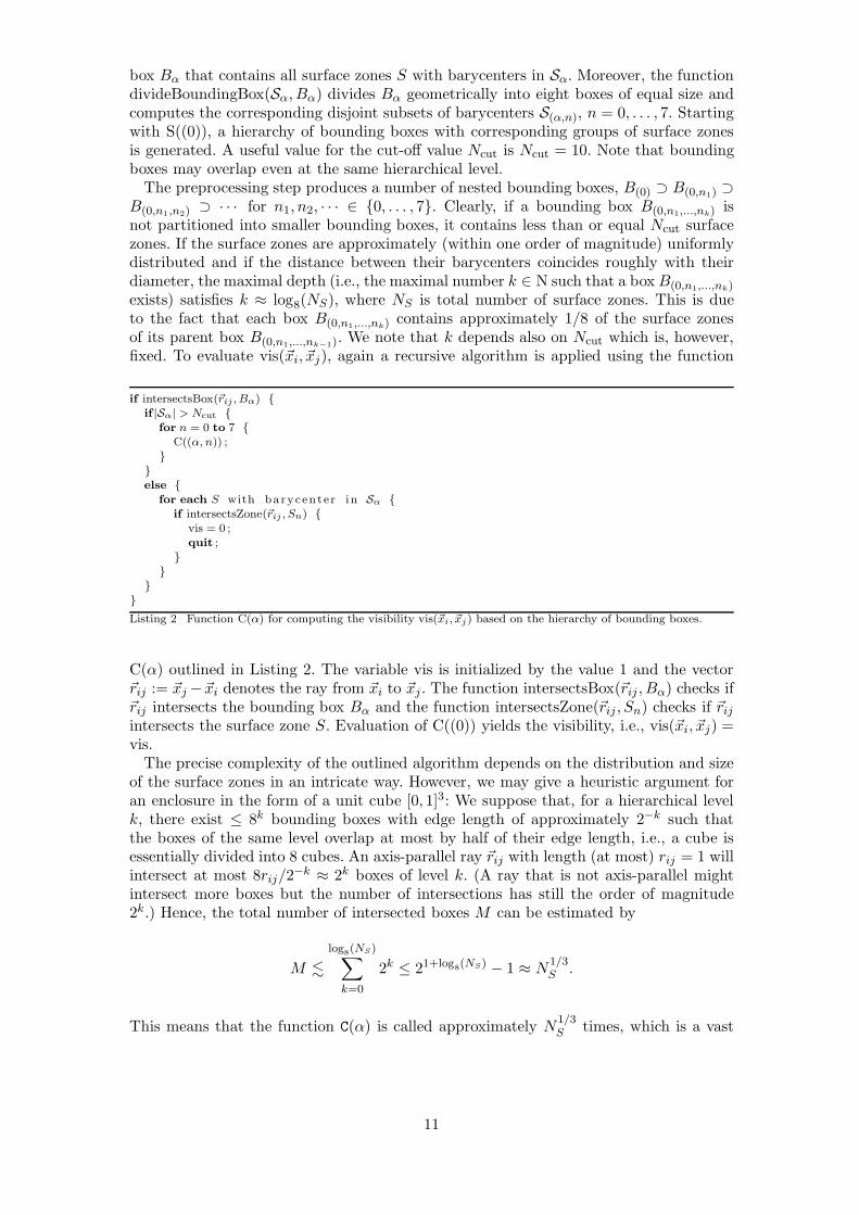
Listing 2 Function C(α) for computing the visibility vis(~xi, ~xj) based on the hierarchy of bounding boxes.

C(α) outlined in Listing 2. The variable vis is initialized by the value 1 and the vector~rij := ~xj −~xi denotes the ray from ~xi to ~xj. The function intersectsBox(~rij , Bα) checks if~rij intersects the bounding box Bα and the function intersectsZone(~rij , Sn) checks if ~rijintersects the surface zone S. Evaluation of C((0)) yields the visibility, i.e., vis(~xi, ~xj) =vis.The precise complexity of the outlined algorithm depends on the distribution and size

of the surface zones in an intricate way. However, we may give a heuristic argument foran enclosure in the form of a unit cube [0, 1]3: We suppose that, for a hierarchical levelk, there exist ≤ 8k bounding boxes with edge length of approximately 2−k such thatthe boxes of the same level overlap at most by half of their edge length, i.e., a cube isessentially divided into 8 cubes. An axis-parallel ray ~rij with length (at most) rij = 1 willintersect at most 8rij/2

−k ≈ 2k boxes of level k. (A ray that is not axis-parallel mightintersect more boxes but the number of intersections has still the order of magnitude2k.) Hence, the total number of intersected boxes M can be estimated by

M .

log8(NS)∑

k=0

2k ≤ 21+log8(NS) − 1 ≈ N

1/3S .

This means that the function C(α) is called approximately N1/3S times, which is a vast

11

improvement compared to the direct approach with approximately NS operations.

3. INTEGRATION WITH TRANSFORMED COORDINATES

In this section, we present coordinate transformations which lead to smooth kernels. Wediscuss only the transformations used for the volume-volume case, i.e., vivj , because thisis the most complex situation. The other cases visj and sisj can be analyzed and treatedin a similar manner.

3.1. Volume-Volume Direct Exchange Areas

We consider the computation of the integral Eq. (17) with k(~xi, ~xj) defined in Eq. (20).We can distinguish between the cases:

• Vi = Vj (Section 3.1.1),• Vi and Vj share a joint face,• Vi and Vj share a joint edge,• Vi and Vj share a joint vertex,• the distance between Vi and Vj is greater than zero (Section 3.1.2).

We describe the method only for the first and the last case. The case Vi = Vj is interesting,because it entails the most severe singularity in the integral kernel. The case where Vi

and Vj are disjoint volumes is shown because it does not entail any singularities. Theother cases follow with similar techniques.

3.1.1. Identical Volumes

For this section, we have to abandon the notation dVi in favor of the rigorous notationd~xi, which specifies the integration variable ~xi. The integration domain is Vi.Let Vi = Vj = [xi1, x

i1 + di1] × [xi2, x

i2 + di2] × [xi3, x

i3 + di3] be an arbitrary axis-parallel

cuboid with corresponding transformations Λi = Λj from Section 2.1. Substitution of Λi

transfers the integral Eq. (17) to the reference volume, i.e.,

vivi =

∫

Vi

∫

Vj

k(~xi, ~xj) d~xi d~xj = |Vi|2

∫

Vref

∫

Vref

k(Λi(~α),Λi(~β)) d~β d~α. (21)

With the relative coordinates ~γ := ~β − ~α = (γ1, γ2, γ3), we write

g(~γ) :=exp(−Ki|(d

i1γ1, d

i2γ2, d

i3γ3)|)

|(di1γ1, di2γ2, d

i3γ3)|

2, f(~α, ~β) := |Vi|

2K2i

πvis(Λi(~α),Λi(~β)). (22)

We define the transformed integral kernel

k(~α, ~β) := |Vi|2k(Λi(~α),Λi(~β)) = g(~β − ~α)f(~α, ~β). (23)

Note that g contains the singular behavior of the integral kernel. Moreover, g and fare symmetric in the sense that g(~γ) = g(−~γ) and f(~α, ~β) = f(~β, ~α), respectively. As

outlined in Fig. 5, we first substitute ~β = ~α+ ~γ. Then,

vivi =

∫

Vref

∫

(Vref−~α)k(~α, ~α+ ~γ) d~γ d~α, (24)

12

~α ∈ Vref

~α ∈ Vref

~α ∈ Vref

~1

~1

~1~1

~0

~0 ~0

~0

~β ∈ Vref

~γ ∈ (Vref − ~α)

~γ ∈ (Vref − ~α)

−~α

−~α

D1D2

Translation ~γ = ~β − ~α

Division into D1–D8

~1− ~αD4

D5 D7

D8

D3

D6

~1− ~α

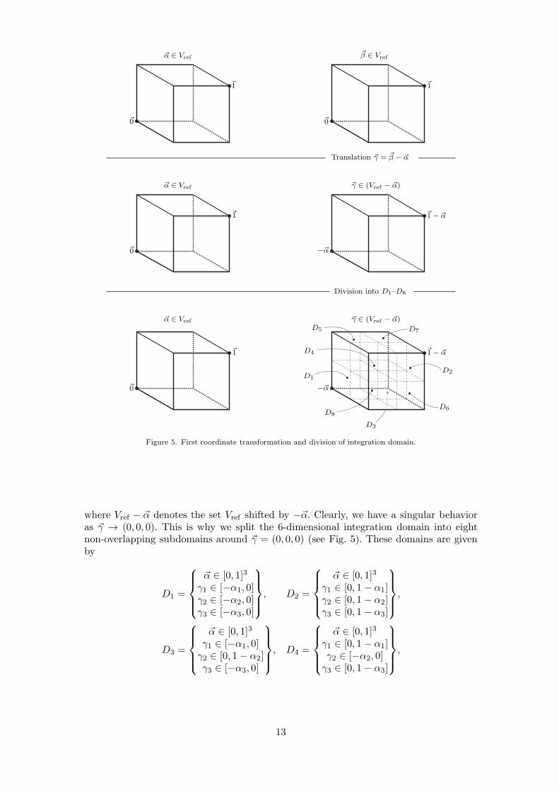
Figure 5. First coordinate transformation and division of integration domain.

where Vref − ~α denotes the set Vref shifted by −~α. Clearly, we have a singular behavioras ~γ → (0, 0, 0). This is why we split the 6-dimensional integration domain into eightnon-overlapping subdomains around ~γ = (0, 0, 0) (see Fig. 5). These domains are givenby

D1 =

~α ∈ [0, 1]3

γ1 ∈ [−α1, 0]γ2 ∈ [−α2, 0]γ3 ∈ [−α3, 0]

, D2 =

~α ∈ [0, 1]3

γ1 ∈ [0, 1 − α1]γ2 ∈ [0, 1 − α2]γ3 ∈ [0, 1 − α3]

,

D3 =

~α ∈ [0, 1]3

γ1 ∈ [−α1, 0]γ2 ∈ [0, 1 − α2]γ3 ∈ [−α3, 0]

, D4 =

~α ∈ [0, 1]3

γ1 ∈ [0, 1 − α1]γ2 ∈ [−α2, 0]γ3 ∈ [0, 1 − α3]

,

13

D5 =

~α ∈ [0, 1]3

γ1 ∈ [−α1, 0]γ2 ∈ [−α2, 0]γ3 ∈ [0, 1 − α3]

, D6 =

~α ∈ [0, 1]3

γ1 ∈ [0, 1 − α1]γ2 ∈ [0, 1 − α2]γ3 ∈ [−α3, 0]

,

D7 =

~α ∈ [0, 1]3

γ1 ∈ [−α1, 0]γ2 ∈ [0, 1 − α2]γ3 ∈ [0, 1 − α3]

, D8 =

~α ∈ [0, 1]3

γ1 ∈ [0, 1 − α1]γ2 ∈ [−α2, 0]γ3 ∈ [−α3, 0]

.

and satisfy⋃8

j=1Dj = Vref × (Vref − ~α). Thus, the integral vivi changes to

vivi =

8∑

j=1

∫

Dj

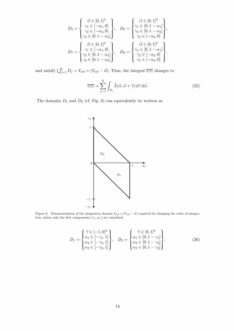
k(~α, ~α+ ~γ) d~γ d~α. (25)

The domains D1 and D2 (cf. Fig. 6) can equivalently be written as

γ1

α1

−γ1

D2

D1

1

1

0

−1

Figure 6. Parametrization of the integration domain Vref × (Vref − ~α) required for changing the order of integra-tion, where only the first components (γ1, α1) are visualized.

D1 =

~γ ∈ [−1, 0]3

α1 ∈ [−γ1, 1]α2 ∈ [−γ2, 1]α3 ∈ [−γ3, 1]

, D2 =

~γ ∈ [0, 1]3

α1 ∈ [0, 1 − γ1]α2 ∈ [0, 1 − γ2]α3 ∈ [0, 1 − γ3]

. (26)

14

D1

~1

~1 ~1

~1 ~1~1

~1

~1~1~1

~1

~1

~1

~1

~1~1

~α ∈ [0, 1−γ1]×[0, 1− γ2]

−~γ

~0

~0 ~0

~0 ~0~0

~0

~0

~0~0~0

~0

~0

~0

~0

~0~0

~γ ∈ −Vref

Coordinate transformation ~γ → −~γ

D2

~γ ∈ Vref~γ ∈ Vref

~γ ∈ Vref

~γ ∈ Vref

~1− ~γ

Coordinate transformation ~α → ~α− ~γ

~γ

~γ

~γ

~γ

g(~γ), f(~α, ~α+ ~γ)g(~γ), f(~α, ~α+ ~γ)

g(~γ) = g(−~γ), f(~α, ~α− ~γ)

W1 W2 W3

W

−~1

g(~γ), f(~α− ~γ, ~α) = f(~α, ~α− ~γ)

~µ ∈ Vref ~ν ∈ VrefΦ−1

1 (~γ, ~α)

~α ∈ [γ1, 1]×[γ2, 1]× [γ3, 1]

~α ∈ [γ1, 1]×[γ2, 1]× [γ3, 1]

~α ∈ [γ1, 1]×[γ2, 1]× [γ3, 1]

~α ∈ Vref ~γ ∈ D1 ∪D2

D1D2

~α ∈ [−γ1, 1]×[−γ2, 1]

· · · similar for Φ−12 (~γ, ~α) and Φ−1

3 (~γ, ~α)

×[−γ3, 1] ×[0, 1−γ3]

−~α

~1− ~α

~γ ∈ [0, 1]×[0, γ1] ~γ ∈ [0, γ2]×[0, 1] ~γ ∈ [0, γ3]×[0, γ3]×[0, γ1] ×[0, γ2] ×[0, 1]

~α ∈ [γ1, 1]×[γ2, 1]×[γ3, 1]

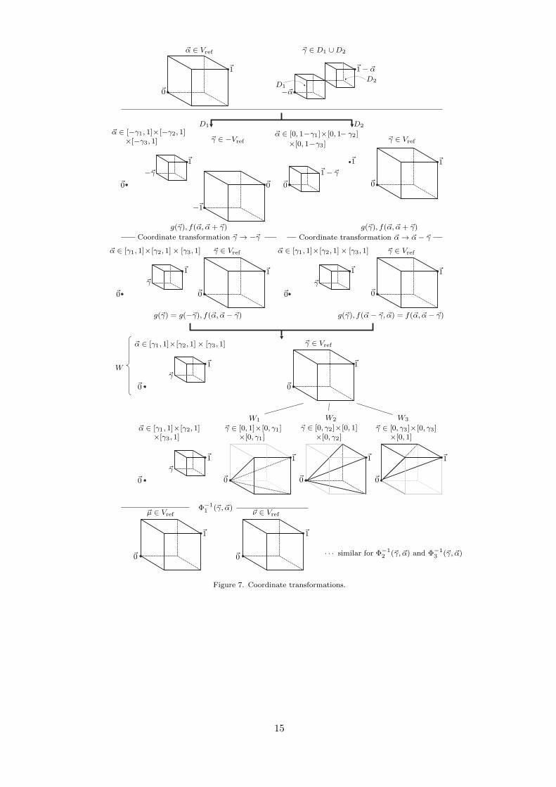
Figure 7. Coordinate transformations.

15

With symmetry of g and f , the coordinate transformations ~γ → −~γ and ~α → ~α − ~γare applied to D1 and D2, respectively (cf. Fig. 7). We get

∫

D1∪D2

k(~α, ~α+ ~γ) d~γ d~α = 2

∫

[0,1]3g(~γ)

∫ 1

γ1

∫ 1

γ2

∫ 1

γ3

f(~α, ~α− ~γ) dα1 dα2 dα3 d~γ, (27)

as indicated in Fig. 7. In this way, we have transformed the integration over D1 ∪ D2

into an integration over

W =

~γ ∈ [0, 1]3

α1 ∈ [γ1, 1]α2 ∈ [γ2, 1]α3 ∈ [γ3, 1]

. (28)

Still, the integrand exhibits a singular behavior for ~γ = (0, 0, 0). To get rid of thissingularity, we will use a special Duffy transformation. To that end, we split the referencevolume Vref = [0, 1]3 for ~γ into three subdomains (pyramides shown in Fig. 7). This givesthe non-overlapping integration domains

W1 =

γ1 ∈ [0, 1]γ2 ∈ [0, γ1]γ3 ∈ [0, γ1]α1 ∈ [γ1, 1]α2 ∈ [γ2, 1]α3 ∈ [γ3, 1]

,W2 =

γ1 ∈ [0, γ2]γ2 ∈ [0, 1]γ3 ∈ [0, γ2]α1 ∈ [γ1, 1]α2 ∈ [γ2, 1]α3 ∈ [γ3, 1]

,W3 =

γ1 ∈ [0, γ3]γ2 ∈ [0, γ3]γ3 ∈ [0, 1]α1 ∈ [γ1, 1]α2 ∈ [γ2, 1]α3 ∈ [γ3, 1]

, (29)

which satisfy W = W1 ∪W2 ∪W3. Each of these subdomains will then be transformedback to the reference volume Vref by a special Duffy transformation. Moreover, we willalso transform the volume [γ1, 1]× [γ2, 1]× [γ3, 1] into Vref .Let Φj with j = 1, 2, 3 denote the functions which transform Vref × Vref = [0, 1]6 into

the domains Wj . The meaning of Φ1 is indicated in Fig. 7. With ~µ = (µ1, µ2, µ3), ~ν =(ν1, ν2, ν3) ∈ Vref , the functions Φj are given by

Φ1(~µ, ~ν) = (µ1, µ1µ2, µ1µ3, µ1 + ν1(1− µ1), µ1µ2 + ν2(1 − µ1µ2), µ1µ3 + ν3(1− µ1µ3)),

Φ2(~µ, ~ν) = (µ1µ2, µ2, µ2µ3, µ1µ2 + ν1(1− µ1µ2), µ2 + ν2(1− µ2), µ2µ3 + ν3(1− µ2µ3)),

Φ3(~µ, ~ν) = (µ1µ3, µ2µ3, µ3, µ1µ3 + ν1(1− µ1µ3), µ2µ3 + ν2(1− µ2µ3), µ3 + ν3(1− µ3)),

The corresponding Jacobian determinants are

|det(∇Φ1(~µ, ~ν))| = µ21(1− µ1)(1 − µ1µ2)(1 − µ1µ3), (30a)

|det(∇Φ2(~µ, ~ν))| = µ22(1− µ1µ2)(1− µ2)(1 − µ2µ3), (30b)

|det(∇Φ3(~µ, ~ν))| = µ23(1− µ1µ3)(1− µ2µ3)(1 − µ3). (30c)

According to the transformation theorem and the Fubini theorem, Eq. (27) can be rewrit-ten in the form

∫

D1∪D2

k(~α, ~α+ ~γ) d~γ d~α = 2

3∑

j=1

∫

Wj

k(~α, ~α − ~γ) d~γ d~α (31)

16

= 2

3∑

j=1

∫

[0,1]6k(Φj(~µ, ~ν)4,5,6,Φj(~µ, ~ν)4,5,6 − Φj(~µ, ~ν)1,2,3)|det(∇Φj(~µ, ~ν))|d~µ d~ν.

Note that the first three components Φi(~µ, ~ν)1,2,3 of Φi(~µ, ~ν) map to the ~γ variable andthe second three components Φi(~µ, ~ν)4,5,6 of Φi(~µ, ~ν) map to the ~α variable. It remains toanalyze the singularity of the integrand in Eq. (31). We consider the singular part g(~γ)from Eq. (27) and multiply it with the determinant of the transformations. This leads to

g(Φ1(~µ, ~ν)1,2,3)|det(∇Φ1(~µ, ~ν))|

=exp(−K|(di1µ1, d

i2µ1µ2, d

i3µ1µ3)|)

|(di1µ1, di2µ1µ2, di3µ1µ3)|2µ21(1− µ1)(1− µ1µ2)(1− µ1µ3)

=exp(−K|(di1µ1, d

i2µ1µ2, d

i3µ1µ3)|)

|(di1, di2µ2, di3µ3)|2

(1− µ1)(1− µ1µ2)(1 − µ1µ3) =: g1(~µ) for µ1 > 0.

For Φ2 and Φ3, we proceed analogously and get

g(Φ2(~µ, ~ν)1,2,3)|det(∇Φ2(~µ, ~ν))|

=exp(−K|(di1µ1µ2, d

i2µ2, d

i3µ2µ3)|)

|(di1µ1, di2, d

i3µ3)|2

(1− µ1µ2)(1− µ2)(1 − µ2µ3) =: g2(~µ) for µ2 > 0,

g(Φ3(~µ, ~ν)1,2,3)|det(∇Φ3(~µ, ~ν))|

=exp(−K|(di1µ1µ3, d

i2µ2µ3, d

i3µ3)|)

|(di1µ1, di2µ2, di3)|2

(1− µ1µ3)(1− µ2µ3)(1− µ3) =: g3(~µ) for µ3 > 0.

Note that the functions g1(~µ), g2(~µ), and g3(~µ) are smooth with respect to ~µ ∈ Vref

because the denominator is strictly positive, i.e., the singularity vanishes by multiplyingg(·) with the Jacobian determinants from Eq. (30).Next, we transform the function f(~α, ~α − ~γ) from Eq. (27) by means of the Φk. For a

compact notation, we define the functions fk1 by

fk1 (~µ, ~ν) := f(Φk(~µ, ~ν)4,5,6,Φk(~µ, ~ν)4,5,6 − Φk(~µ, ~ν)1,2,3).

For the remaining domains D3 ∪D4, D5 ∪D6, D7 ∪D8 we proceed similarly. We stressthat the functions gk(·) are the same for the other domains but the functions fk

1 differslightly. We use the notation fk

2 for the case D3∪D4, fk3 for D5∪D6, and fk

4 for D7∪D8.Finally, the integral from Eq. (25) becomes

vivi =

8∑

j=1

∫

Dj

k(~α, ~α+ ~γ) d~γ d~α = 2

∫

Vref

3∑

k=1

gk(~µ)

∫

Vref

4∑

ℓ=1

fkℓ (~µ, ~ν) d~ν d~µ, (32)

with gk being smooth. However, the functions fkℓ are in general not analytic because

f(~α, ~β) contains the non-analytic factor vis(Λi(~α),Λi(~β)) ∈ {0, 1} (cf. Eq. (22)). For thespecial case vis ≡ 1, Eq. (32) simplifies to

vivi =8|Vi|

2K2i

π

∫

Vref

3∑

k=1

gk(~µ) d~µ, (33)

17

i. e., the 6-fold integral reduces to a 3-fold integral with a smooth integrand.Generally, the integrals in Eq. (32) are computable with straightforward Gaussian

quadrature from Eq. (19), i.e.,

vivi ≈ 2

3∑

k=1

M∑

k1=0

M∑

k2=0

M∑

k3=0

wk1wk2

wk3gk(sk1

, sk2, sk3

)×

×4∑

ℓ=0

M∑

k4=0

M∑

k5=0

M∑

k6=0

wk4wk5

wk6fkℓ (sk1

, sk2, sk3

, sk4, sk5

, sk6).

3.1.2. Volumes with Positive Distance

Again, we transform the integral (17) onto the reference volume Vref by use of the trans-formations Λi and Λj from Section 2.1, i.e.,

vivj =

∫

Vi

∫

Vj

k(~xi, ~xj) d~xi d~xj = |Vi||Vj |

∫

Vref

∫

Vref

k(Λi(~α),Λj(~β)) d~β d~α. (34)

The integral kernel k(Λi(~α),Λj(~β)) from Eq. (20) does not have singularities because

|Λi(~α) − Λj(~β)| > 0 for all ~α, ~β ∈ Vref . Therefore, we may straightforwardly apply theGaussian quadrature from Eq. (19) to evaluate the integral, i.e.,

vivj ≈ |Vi||Vj |M∑

k=0

M∑

ℓ=0

M∑

m=0

M∑

n=0

M∑

p=0

M∑

q=0

wkwℓwmwnwpwqk(Λi(sk, sℓ, sm),Λj(sn, sp, sq)).

As mentioned at the beginning of this section, the derivation of quadrature formulaefor the cases where Vi 6= Vj and Vi ∩ Vj is a common face, edge, or vertex is similar tothe given derivation for the case Vi = Vj. The following theorem can be proved along thelines of [21, Section 5.3.2.4] and holds for all cases.

Theorem 3.1: Let vivj denote the approximation of the direct exchange area vivj by

Duffy transformation and Gaussian quadrature of order M as described in Section 3.1.1

for Vi = Vj or by direct Gaussian quadrature of order M as described in Section 3.1.2

for Vi ∩ Vj = ∅. Assume vis = 1. Then, there holds

|vivj − vivj| ≤ C|Vi||Vj | exp(−M),

where C > 0 depends only on dik, djk for k = 1, 2, 3. If the distance d between Vi and Vj

is strictly positive, then C depends additionally on d.

4. Example Problems

In this section, we present two example problems and a case study. The results demon-strate the accuracy, the low computational effort, and the applicability of the method tolarge-scale problems. In the first example problem, a non-convex geometry is analyzedand the results are validated based on satisfaction of the summation rules Eq. (15). Inthe second example, a benchmark problem is solved and the results are validated bycomparison to values published in the literature. The case study demonstrates how themethod can be utilized in a simulation model of an industrial strip annealing furnace.

18

0 0.2 0.4 0.6 0.8 1 0

0.5

1

1.5

2

0

0.2

0.4

0.6

0.8

1

1.2

1.4

1.6

1.8

2

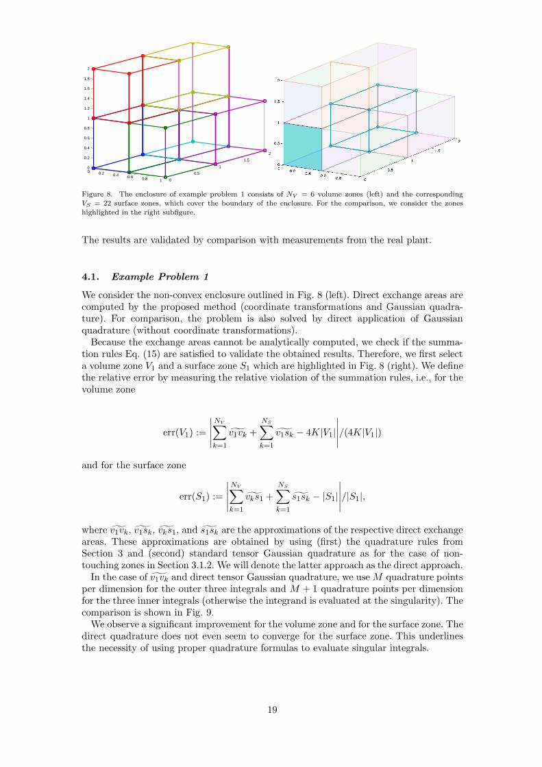
Figure 8. The enclosure of example problem 1 consists of NV = 6 volume zones (left) and the correspondingVS = 22 surface zones, which cover the boundary of the enclosure. For the comparison, we consider the zoneshighlighted in the right subfigure.

The results are validated by comparison with measurements from the real plant.

4.1. Example Problem 1

We consider the non-convex enclosure outlined in Fig. 8 (left). Direct exchange areas arecomputed by the proposed method (coordinate transformations and Gaussian quadra-ture). For comparison, the problem is also solved by direct application of Gaussianquadrature (without coordinate transformations).Because the exchange areas cannot be analytically computed, we check if the summa-

tion rules Eq. (15) are satisfied to validate the obtained results. Therefore, we first selecta volume zone V1 and a surface zone S1 which are highlighted in Fig. 8 (right). We definethe relative error by measuring the relative violation of the summation rules, i.e., for thevolume zone

err(V1) :=

∣∣∣∣∣

NV∑

k=1

v1vk +

NS∑

k=1

v1sk − 4K|V1|

∣∣∣∣∣/(4K|V1|)

and for the surface zone

err(S1) :=

∣∣∣∣∣

NV∑

k=1

vks1 +

NS∑

k=1

s1sk − |S1|

∣∣∣∣∣/|S1|,

where v1vk, v1sk, vks1, and s1sk are the approximations of the respective direct exchangeareas. These approximations are obtained by using (first) the quadrature rules fromSection 3 and (second) standard tensor Gaussian quadrature as for the case of non-touching zones in Section 3.1.2. We will denote the latter approach as the direct approach.In the case of v1vk and direct tensor Gaussian quadrature, we use M quadrature points

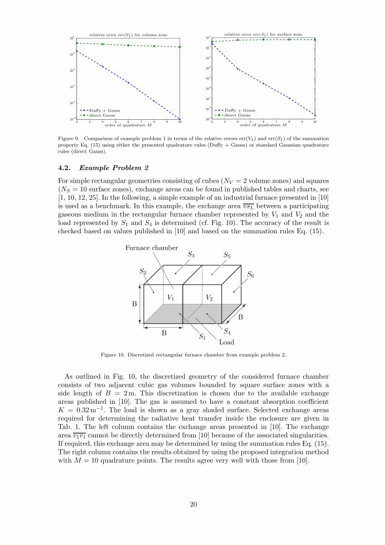
per dimension for the outer three integrals and M + 1 quadrature points per dimensionfor the three inner integrals (otherwise the integrand is evaluated at the singularity). Thecomparison is shown in Fig. 9.We observe a significant improvement for the volume zone and for the surface zone. The

direct quadrature does not even seem to converge for the surface zone. This underlinesthe necessity of using proper quadrature formulas to evaluate singular integrals.

19

2 3 4 5 6 7 8 9 1010

−10

10−8

10−6

10−4

10−2

100

order of quadrature M

Duffy + Gaussdirect Gauss

relative error err(V1) for volume zone

2 3 4 5 6 7 8 9 1010

−9

10−8

10−7

10−6

10−5

10−4

10−3

10−2

10−1

order of quadrature M

Duffy + Gaussdirect Gauss

relative error err(S1) for surface zone

Figure 9. Comparison of example problem 1 in terms of the relative errors err(V1) and err(S1) of the summationproperty Eq. (15) using either the presented quadrature rules (Duffy + Gauss) or standard Gaussian quadraturerules (direct Gauss).

4.2. Example Problem 2

For simple rectangular geometries consisting of cubes (NV = 2 volume zones) and squares(NS = 10 surface zones), exchange areas can be found in published tables and charts, see[1, 10, 12, 25]. In the following, a simple example of an industrial furnace presented in [10]is used as a benchmark. In this example, the exchange area vsL between a participatinggaseous medium in the rectangular furnace chamber represented by V1 and V2 and theload represented by S1 and S4 is determined (cf. Fig. 10). The accuracy of the result ischecked based on values published in [10] and based on the summation rules Eq. (15).

B

B

B

V1 V2

S1

S2

S3

S4

S5

S6

Furnace chamber

Load

Figure 10. Discretized rectangular furnace chamber from example problem 2.

As outlined in Fig. 10, the discretized geometry of the considered furnace chamberconsists of two adjacent cubic gas volumes bounded by square surface zones with aside length of B = 2m. This discretization is chosen due to the available exchangeareas published in [10]. The gas is assumed to have a constant absorption coefficientK = 0.32m−1. The load is shown as a gray shaded surface. Selected exchange areasrequired for determining the radiative heat transfer inside the enclosure are given inTab. 1. The left column contains the exchange areas presented in [10]. The exchangearea v1v1 cannot be directly determined from [10] because of the associated singularities.If required, this exchange area may be determined by using the summation rules Eq. (15).The right column contains the results obtained by using the proposed integration methodwith M = 10 quadrature points. The results agree very well with those from [10].

20

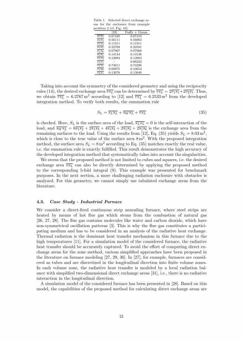
Table 1. Selected direct exchange ar-eas for the enclosure from exampleproblem 2 (cf. Fig. 10).

[10] Duffy + Gausss1s2 0.67420 0.67410s1s3 0.56111 0.56063s1s4 0.11911 0.11911s1s5 0.22709 0.22581s1s6 0.07967 0.07968s2s6 0.14144 0.14136v1v2 0.12084 0.12084v1v1 - 0.66222v1s1 0.74611 0.74296v1s6 0.09975 0.10054v2s1 0.13078 0.13040

Taking into account the symmetry of the considered geometry and using the reciprocityrules (14), the desired exchange area vsL can be determined by vsL = 2v1s1+2v2s1. Thus,we obtain vsL = 6.2767m2 according to [12] and vsL = 6.2533m2 from the developedintegration method. To verify both results, the summation rule

SL = sLsL + sW sL + vsL (35)

is checked. Here, SL is the surface area of the load, sLsL = 0 is the self-interaction of theload, and sW sL = 6s1s2 + 2s1s3 + 4s1s4 + 2s1s5 + 2s1s6 is the exchange area from theremaining surfaces to the load. Using the results from [12], Eq. (35) yields SL = 8.03m2,which is close to the true value of the surface area 8m2. With the proposed integrationmethod, the surface area SL = 8m2 according to Eq. (35) matches exactly the real value,i.e. the summation rule is exactly fulfilled. This result demonstrates the high accuracy ofthe developed integration method that systematically takes into account the singularities.We stress that the proposed method is not limited to cubes and squares, i.e. the desired

exchange area vsL can also be directly determined by applying the proposed methodto the corresponding 5-fold integral (9). This example was presented for benchmarkpurposes. In the next section, a more challenging radiation enclosure with obstacles isanalyzed. For this geometry, we cannot simply use tabulated exchange areas from theliterature.

4.3. Case Study - Industrial Furnace

We consider a direct-fired continuous strip annealing furnace, where steel strips areheated by means of hot flue gas which stems from the combustion of natural gas[26, 27, 28]. The flue gas contains molecules like water and carbon dioxide, which havenon-symmetrical oscillation patterns [3]. This is why the flue gas constitutes a partici-pating medium and has to be considered in an analysis of the radiative heat exchange.Thermal radiation is the dominant heat transfer mechanism in this furnace due to thehigh temperatures [11]. For a simulation model of the considered furnace, the radiativeheat transfer should be accurately captured. To avoid the effort of computing direct ex-change areas for the zone method, various simplified approaches have been proposed inthe literature on furnace modeling [27, 29, 30]. In [27], for example, furnaces are consid-ered as tubes and are discretized in the longitudinal direction into finite volume zones.In each volume zone, the radiative heat transfer is modeled by a local radiation bal-ance with simplified two-dimensional direct exchange areas [31], i.e., there is no radiativeinteraction in the longitudinal direction.A simulation model of the considered furnace has been presented in [28]. Based on this

model, the capabilities of the proposed method for calculating direct exchange areas are

21

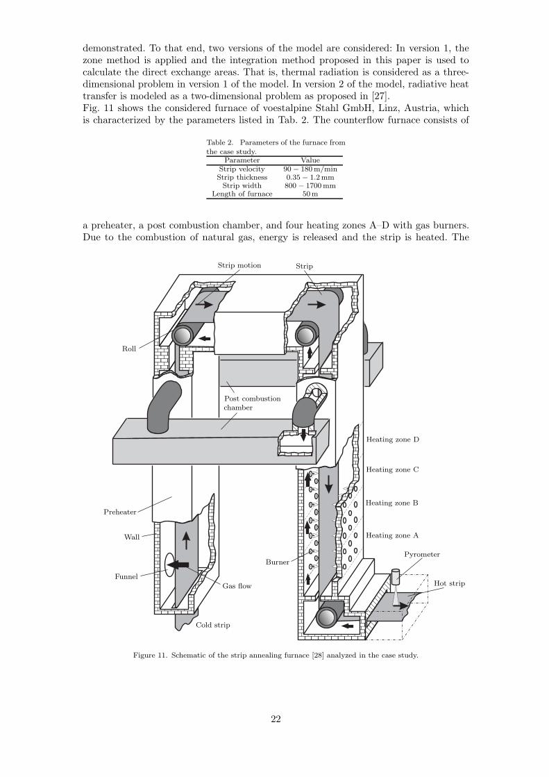
demonstrated. To that end, two versions of the model are considered: In version 1, thezone method is applied and the integration method proposed in this paper is used tocalculate the direct exchange areas. That is, thermal radiation is considered as a three-dimensional problem in version 1 of the model. In version 2 of the model, radiative heattransfer is modeled as a two-dimensional problem as proposed in [27].Fig. 11 shows the considered furnace of voestalpine Stahl GmbH, Linz, Austria, whichis characterized by the parameters listed in Tab. 2. The counterflow furnace consists of

Table 2. Parameters of the furnace fromthe case study.

Parameter ValueStrip velocity 90− 180m/minStrip thickness 0.35− 1.2mmStrip width 800 − 1700mm

Length of furnace 50m

a preheater, a post combustion chamber, and four heating zones A–D with gas burners.Due to the combustion of natural gas, energy is released and the strip is heated. The

aaaaaaaaaaaaaa

aaaaaaaaaaaaaa

aaaaaaaaaaaaaaaaaaaaaaaaaaaaaaaaaaaaaaaaaaaa

aa

aaaaaaaaaaaaaaaaaa

aaaaaaaaaaaaaaaaaaaa

aaaaaaaaaaaaaaaaaaaaaaaaaaaaaaaaaaaaaaaa

aaaaaaaaaaaaaaaaaa

aaaaaaaaaaaaaaaaaaaaaaaaaaaaaa

aaaaaaaaaaaaaaaaaaaaaaaaaaaaaaaaaa

aaaaaaaaaaaaaaaaaaaa

aaaaaaaaaaaaaa

aaaaaaaaaaaaaaaaaaaaaa

aaaaaaaaaaaaaaaaaaaaaaaaa

aaaaaaaaaaaaaaaaaaaaaaaaaaaaaaaaaaaaaaaaaaaaaaaaaaaaaaaaaaaaaaaaaaaaaaaaaaaaaaaaaaaa

aaaaaaaaaaaaaaaaaaaaaaaaaaaaaa

aaaaaaaaaaaaaaaa

aaaaaaaaaaaaaaaaaaaaaaaaaaaaaaaaaaaaaaaaaaaaaaaaaaaaaaaaaaaaaaaaaaaaaaaaaaaaaaaaaaaaaaaaaaaaaaaaaaaaaaaaaaaaaaaaaaaaaaaaaaaaaaaaaaaaaaaaaaaaaaaaaaaaaaaaaaaaaaaaaaaaaaaaaaaaaaaaaaaaaaaaaaaaaaaaaaaaaaaaaaaaaaaaaaaaaaaaaaaaaaaaaaaaaaaaaaaaaaaaaaaaaaaaaaaaaaaaaaaaaaaaaaaaaaaaaaaaaaaaaaaaaa

aaaaaaaaaaaaaaaaaaaaaa

aaaaaaaaaaaaaaaaaaaaaaaaaaaaaaaaaaaaaaaaaaaa

aaa aa

aaaa

aaaaaa

Hot strip

Heating zone A

Heating zone B

Gas flow

Heating zone C

Heating zone D

Preheater

Post combustion

Roll

Funnel

Cold strip

Strip

Wall

Strip motion

BurnerPyrometer

chamber

Figure 11. Schematic of the strip annealing furnace [28] analyzed in the case study.

22

strip is conveyed through the furnace by three rolls. At the end of the furnace, the striptemperature is measured by a pyrometer. Additionally, thermocouples are installed inthe heating zones to measure the local wall temperatures.In Sec. 4.3.1, an overview of the simulation model is given. A simulation study is carriedout based on both versions of the model. In Section 4.3.2, the model is verified by meansof measurements from the real plant.

4.3.1. Overview of the Simulation Model

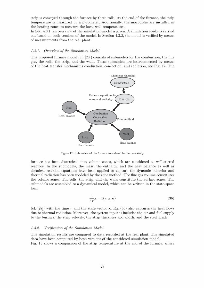
The proposed furnace model (cf. [28]) consists of submodels for the combustion, the fluegas, the rolls, the strip, and the walls. These submodels are interconnected by meansof the heat transfer mechanisms conduction, convection, and radiation, see Fig. 12. The

Chemical reactions

Balance equations for

Combustion

Roll

mass and enthalpy Flue gas

Heat balance

Heat balance

Heat balance

Conduction

Radiation

Strip

Convection

Wall

Zone method

Figure 12. Submodels of the furnace considered in the case study.

furnace has been discretized into volume zones, which are considered as well-stirredreactors. In the submodels, the mass, the enthalpy, and the heat balance as well aschemical reaction equations have been applied to capture the dynamic behavior andthermal radiation has been modeled by the zone method. The flue gas volume constitutesthe volume zones. The rolls, the strip, and the walls constitute the surface zones. Thesubmodels are assembled to a dynamical model, which can be written in the state-spaceform

d

dτx = f(τ,x,u) (36)

(cf. [28]) with the time τ and the state vector x. Eq. (36) also captures the heat flowsdue to thermal radiation. Moreover, the system input u includes the air and fuel supplyto the burners, the strip velocity, the strip thickness and width, and the steel grade.

4.3.2. Verification of the Simulation Model

The simulation results are compared to data recorded at the real plant. The simulateddata have been computed by both versions of the considered simulation model.Fig. 13 shows a comparison of the strip temperature at the end of the furnace, where

23

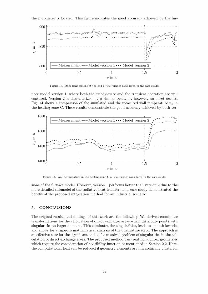
the pyrometer is located. This figure indicates the good accuracy achieved by the fur-

0 0.5 1 1.5 2

800

850

900

τ in h

t sin

K

Measurement Model version 1 Model version 2

Figure 13. Strip temperature at the end of the furnace considered in the case study.

nace model version 1, where both the steady-state and the transient operation are wellcaptured. Version 2 is characterized by a similar behavior, however, an offset occurs.Fig. 14 shows a comparison of the simulated and the measured wall temperature tw inthe heating zone C. These results demonstrate the good accuracy achieved by both ver-

0 0.5 1 1.5 21400

1450

1500

1550

τ in h

t win

K

Measurement Model version 1 Model version 2

Figure 14. Wall temperature in the heating zone C of the furnace considered in the case study.

sions of the furnace model. However, version 1 performs better than version 2 due to themore detailed submodel of the radiative heat transfer. This case study demonstrated thebenefit of the proposed integration method for an industrial scenario.

5. CONCLUSIONS

The original results and findings of this work are the following: We derived coordinatetransformations for the calculation of direct exchange areas which distribute points withsingularities to larger domains. This eliminates the singularities, leads to smooth kernels,and allows for a rigorous mathematical analysis of the quadrature error. The approach isan effective cure for the significant and so-far unsolved problem of singularities in the cal-culation of direct exchange areas. The proposed method can treat non-convex geometrieswhich require the consideration of a visibility function as mentioned in Section 2.2. Here,the computational load can be reduced if geometry elements are hierarchically clustered.

24

In case of constant visibility (i.e. vis = 1), the integral reduces to a lower dimensionalintegral. The developed method was validated based on numerical results, results pub-lished in the literature, and measurements from an industrial plant. The method is notrestricted to the computation of direct exchange areas and may be utilized in a similarway for more general singular integral kernels.

ACKNOWLEDGMENT

This research was financially supported by the Austrian Research Promotion Agency(FFG), grant no.: 834305. Moreover, the authors are grateful to the industrial re-search partners voestalpine Stahl GmbH and Andritz AG. The research of the au-thors MF, TF, and DP is supported through the FWF project Adaptive Boundary El-

ement Method, funded by the Austrian Science fund (FWF) under grant P21732, seehttp://www.asc.tuwien.ac.at/abem. The authors MF and DP acknowledge the sup-port of the FWF doctoral program “Dissipation and Dispersion in Nonlinear PDEs”

under grant W1245, see http://npde.tuwien.ac.at/. The author AS gratefully ac-knowledges financial support provided by the Austrian Academy of Sciences in the formof an APART-fellowship at the Automation and Control Institute of Vienna Universityof Technology.

REFERENCES

1. H.C. Hottel and E.S. Cohen. Radiant heat exchange in a gas filled enclosure: Allowance fornon-uniformity of gas temperature. American Institute of Chemical Engineering Journal,4:3–14, 1958.

2. R. Siegel and J.R. Howell. Thermal Radiation Heat Transfer. Taylor & Francis, New York,London, 4th edition, 2002.

3. M.F. Modest. Radiative Heat Transfer. Academic Press, New York, 2nd edition, 2003.4. H.C. Hottel and A.F. Sarofim. Radiative Transfer. McGraw-Hill, New York, 1967.5. H.D. Baehr and K. Stephan. Heat and Mass Transfer. Springer, Berlin Heidelberg, 2nd

edition, 2006.6. A. Faghri, Y. Zhang, and J.R. Howell. Advanced Heat and Mass Transfer. Global Digital

Press, Columbia, MO, 2010.7. J.R. Howell. Thermal radiation in participating media: The past, the present, and some

possible futures. Transactions of the ASME, Journal of Heat Transfer, 110(4b):1220–1229,1988.

8. Y.S. Kocaefe, A. Charette, and M. Munger. Comparison of the various methods for analysingthe radiative heat transfer in furnaces. Proceedings of the Combustion Institute Canadian

Section Spring Technical Meeting, Vancouver, Canada, pages 15–17, May 1987.9. S.C. Mishra and M. Prasad. Radiative heat transfer in participating media – A review.

Sadhana - Academy Proceedings in Engineering Sciences, 23(2):213–232, 1998.10. J.M. Rhine and R.J. Tucker. Modelling of Gas-Fired Furnaces and Boilers and Other Indus-

trial Heating Processes. McGraw-Hill, London, UK, 1991.11. R. Viskanta and M.P. Menguc. Radiation heat transfer in combustion systems. Progress in

Energy and Combustion Science, 13(2):97–160, 1987.12. R.J. Tucker. Direct exchange areas for calculating radiation transfer in rectangular furnaces.

Transactions of the ASME, Journal of Heat Transfer, 108(3):707–710, 1986.13. H. Errku. Radiant heat exchange in gas-filled slabs and cylinders. PhD thesis, Massachusetts

Institute of Technology, Cambridge, MA, 1959.14. W. Tian and W.K.S. Chiu. Calculation of direct exchange areas for nonuniform zones us-

ing a reduced integration scheme. Transactions of the ASME, Journal of Heat Transfer,125(5):839–844, 2003.

25

15. J. Sika. Evaluation of direct-exchange areas for a cylindrical enclosure. Transactions of the

ASME, Journal of Heat Transfer, 113(4):1040–1044, 1991.16. W. Tian and W.K.S. Chiu. Hybrid method to calculate direct exchange areas using the

finite volume method and midpoint intergration. Transactions of the ASME, Journal of

Heat Transfer, 127(8):911–917, 2005.17. J.C. Chai, J.P. Moder, and K.C. Karki. A procedure for view factor calculation using the

finite-volume method. Numerical Heat Transfer, Part B: Fundamentals, 40(1):23–35, 2001.18. H. Ebrahimi, A. Zamaniyan, J.S.S. Mohammadzadeh, and A.A. Khalili. Zonal modeling

of radiative heat transfer in industrial furnaces using simplified model for exchange areacalculation. Applied Mathematical Modelling, 37(16-17):8004–8015, 2013.

19. A. Kheiri, J.L. Tanguier, D. Bour, R. Mainard, and J. Kleinclauss. Transfert de chaleur dansles milieux semi-transparents: adaptation de la methode des zones de Hottel aux milieuxoptiquement epais. Proceeding of the SFT-90 Colloque de Thermique, Nantes, France, 2:37–40, May 1990.

20. J.M. Goyheneche and J.F. Sacadura. The zone method: A new explicit matrix relation tocalculate the total exchange areas in anisotropically scattering medium bounded by anisotrop-ically reflecting walls. Transactions of the ASME, Journal of Heat Transfer, 124(4):696–703,2002.

21. S.A. Sauter and C. Schwab. Boundary Element Methods, volume 39 of Springer Series in

Computational Mathematics. Springer-Verlag, Berlin, 2011.22. L. Greengard and V. Rokhlin. A fast algorithm for particle simulations. J. Comput. Phys.,

73(2):325–348, 1987.23. H. Cheng, L. Greengard, and V. Rokhlin. A fast adaptive multipole algorithm in three

dimensions. J. Comput. Phys., 155(2):468–498, 1999.24. S. Borm, L. Grasedyck, and W. Hackbusch. Introduction to hierarchical matrices with ap-

plications. Engineering Analysis with Boundary Elements, 27(5):405 – 422, 2003.25. H.B. Becker. A mathematical solution for gas-to-surface radiative exchange area for a rectan-

gular parallelepiped enclosure containing a gray medium. Journal of Heat Transfer, 99:203–207, May 1977.

26. K.S. Chapman, S. Ramadhyani, and R. Viskanta. Modeling and analysis of heat transferin a direct-fired continuous reheating furnace. Heat Transfer In Combustion Systems, pages35–44, 1989.

27. D. Marlow. Modelling direct-fired annealing furnaces for transient operations. Applied Math-

ematical Modelling, 20(1):34–40, 1996.28. S. Strommer, M. Niederer, S. Steinboeck, and A. Kugi. A mathematical model of a direct-

fired continuous strip annealing furnace. International Journal for Heat and Mass Transfer,69:375–389, 2014.

29. A. Jaklic, F. Vode, and T. Kolenko. Online simulation model of the slab-reheating processin a pusher-type furnace. Applied Thermal Engineering, 27:1105–1114, 2007.

30. C.-K. Tan, J. Jenkins, J. Ward, J. Broughton, and A. Heeley. Zone modelling of the ther-mal performances of a large-scale bloom reheating furnace. Applied Thermal Engineering,50:1111–1118, 2013.

31. J.P. Holman. Heat Transfer, volume 10. McGraw Hill, 2010.

26