Priv’IT: Private and Sample Efficient Identity Testing

Bryan CaiEECS, MIT

bcai@mit.edu

Constantinos DaskalakisEECS and CSAIL, MITcostis@csail.mit.edu

Gautam KamathEECS and CSAIL, MIT

g@csail.mit.edu

June 8, 2017

Abstract

We develop differentially private hypothesis testing methods for the small sample regime. Given asample D from a categorical distribution p over some domain Σ, an explicitly described distribution qover Σ, some privacy parameter ε, accuracy parameter α, and requirements βI and βII for the type I andtype II errors of our test, the goal is to distinguish between p = q and dTV(p, q) ≥ α.

We provide theoretical bounds for the sample size |D| so that our method both satisfies (ε, 0)-differential privacy, and guarantees βI and βII type I and type II errors. We show that differentialprivacy may come for free in some regimes of parameters, and we always beat the sample complexityresulting from running the χ2-test with noisy counts, or standard approaches such as repetition forendowing non-private χ2-style statistics with differential privacy guarantees. We experimentally com-pare the sample complexity of our method to that of recently proposed methods for private hypothesistesting [GLRV16, KR17].

1 Introduction

Hypothesis testing is the age-old problem of deciding whether observations from an unknown phenomenonp conform to a model q. Often p can be viewed as a distribution over some alphabet Σ, and the goal isto determine, using samples from p, whether it is equal to some model distribution q or not. This type oftest is the lifeblood of the scientific method and has received tremendous study in statistics since its verybeginnings. Naturally, the focus has been on minimizing the number of observations from the unknowndistribution p that are needed to determine, with confidence, whether p = q or p 6= q.

In several fields of research and application, however, samples may contain sensitive information aboutindividuals; consider for example, individuals participating in some clinical study of a disease that carriessocial stigma. It may thus be crucial to guarantee that operating on the samples needed to test a statisticalhypothesis protects sensitive information about the samples. This is not at odds with the goal of hypothesistesting itself, since the latter is about verifying a property of the population p from which the samples aredrawn, and not of the samples themselves.

Without care, however, sensitive information about the sample might actually be divulged by statisticalprocessing that is improperly designed. As recently exhibited, for example, it may be possible to determinewhether individuals participated in a study from data that would typically be published in genome-wideassociation studies [HSR+08]. Motivated in part by this realization, there has been increased recent interestin developing data sharing techniques which are private [JS13, USF13, YFSU14, SSB16].

Protecting privacy when computing on data has been extensively studied in several fields ranging fromstatistics to diverse branches of computer science including algorithms, cryptography, database theory, andmachine learning; see, e.g., [Dal77, AW89, AA01, DN03, Dwo08, DR14] and their references. A notion ofprivacy proposed by theoretical computer scientists which has found a lot of traction is that of differentialprivacy [DMNS06]. Roughly speaking, it requires that the output of an algorithm on two neighboringdatasets D and D′ that differ in the value of one element be statistically close. For a formal definition seeSection 2.

Our goal in this paper is to develop tools for privately performing statistical hypothesis testing. Inparticular, we are interested in studying the tradeoffs between statistical accuracy, power, significance, and

1

arX

iv:1

703.

1012

7v3

[cs

.DS]

7 J

un 2

017

privacy in the sample size. To be precise, given samples from a categorical distribution p over some domainΣ, an explicitly described distribution q over Σ, some privacy parameter ε, accuracy parameter α, andrequirements βI and βII for the type I and type II errors of our test, the goal is to distinguish betweenp = q and dTV(p, q) ≥ α. We want that the output of our test be (ε, 0)-differentially private, and that theprobability we make a type I or type II error be βI and βII respectively. Treating these as hard constraints,we want to minimize the number of samples that we draw from p.

Notice that the correctness constraint on our test pertains to whether we draw the right conclusion abouthow p compares to q, while the privacy constraint pertains to whether we respect the privacy of the samplesthat we draw from p. The pertinent question is how much the privacy constraint increases the number ofsamples that are needed to guarantee correctness. Our main result is that privacy may come for free incertain regimes of parameters, and has a mild cost for all regimes of parameters.

To be precise, without privacy constraints, it is well known that identity testing can be performed

from O(√n

α2 · log 1β ) samples, where n is the size of Σ and β = minβI, βII, and that this is tight [BFF+01,

Pan08, VV14, ADK15]. Our main theoretical result is that, with privacy constraints, the number of samplesthat are needed is

O

(max

√n

α2,

√n

α3/2ε,

n1/3

α5/3ε2/3

· log(1/β)

). (1)

Our statistical test is provided in Section 5 where the above upper bound on the number of samples thatit requires is proven as Theorem 3. Notice that privacy comes for free when the privacy requirement ε isΩ(√α) – for example when ε = 10% and the required statistical accuracy is 3%.

The precise constants sitting in the O(·) notation of Eq. (1) are given in the proof of Theorem 3. Weexperimentally verify the sample efficiency of our tests by comparing them to recently proposed privatestatistical tests [GLRV16, KR17], discussed in more detail shortly. Fixing a differential privacy and type I,type II error constraints, we compare how many samples are required by our and their methods to distinguishbetween hypotheses that are α = 0.1 apart in total variation distance. We find that different algorithms aremore efficient depending on the regime and properties desired by the analyst. Our experiments and furtherdiscussion of the tradeoffs are presented in Section 6.

Approach. A standard approach to turn an algorithm differentially private is to use repetition. As alreadymentioned above, absent differential privacy constraints, statistical tests have been provided that use an

optimal m = O(√n

α2 · log 1β ) number of samples. A trivial way to get (ε, 0)-differential privacy using such a

non-private test is to create O(1/ε) datasets, each comprising m samples from p, and run the non-privatetest on one of these datasets, chosen randomly. It is clear that changing the value of a single element inthe combined dataset may only affect the output of the test with probability at most ε. Thus the output is(ε, 0)-differentially private; see Section 3 for a proof. The issue with this approach is that the total number

of samples that it draws is m/ε = O(√n

εα2 · log 1β ), which is higher than our target. See Corollary 1.

A different approach towards private hypothesis testing is to look deeper into the non-private tests and tryto “privatize” them. The most sample-efficient tests are variations of the classical χ2-test. They computethe number of times, Ni, that element i ∈ Σ appears in the sample and aggregate those counts using astatistic that equals, or is close to, the χ2-divergence between the empirical distribution defined by thesecounts and the hypothesis distribution q. They accept q if the statistic is low and reject q if it is high, usingsome threshold.

A reasonable approach to privatize such a test is to add noise, e.g. Laplace(1/ε) noise, to each countNi, before running the test. It is well known that adding Laplace(1/ε) noise to a set of counts makes themdifferentially private, see Theorem 1. However, it also increases the variance of the statistic. This has beennoticed empirically in recent work of [GLRV16] for the χ2-test. We show that the variance of the optimal χ2-style test statistic significantly increases if we add Laplace noise to the counts, in Section 4.1, thus increasingthe sample complexity from O(

√n) to Ω(n3/4). So this route, too, seems problematic.

A last approach towards designing differentially private tests is to exploit the distance beween the nulland the alternative hypotheses. A correct test should accept the null with probability close to 1, and rejectan alternative that is α-far from the null with probability close to 1, but there are no requirements forcorrectness when the alternative is very close to the null. We could thus try to interpolate smoothly between

2

datasets that we expect to see when sampling the null and datasets that we expect to see when sampling analternative that is far from the null. Rather than outputting “accept” or “reject” by merely thresholding ourstatistic, we would like to tune the probability that we output “reject” based on the value of our statistic, andmake it so that the “reject” probability is ε-Lipschitz as a function of the dataset. Moreover, the probabilityshould be close to 0 on datasets that we expect to see under the null and close to 1 on datasets that weexpect to see under an alternative that is α-far. As we show in Section 4.2, χ2-style statistics have highsensitivity, requiring ω(

√n) samples to be made appropriately Lipschitz.

While both the approach of adding noise to the counts, and that of turning the output of the test Lipschitzfail in isolation, our test actually goes through by intricately combining these two approaches. It has twosteps:

1. A filtering step, whose goal is to “reject” when p is blatantly far from q. This step is performed bycomparing the counts Ni with their expectations under q, after having added Laplace(1/ε) noise tothese counts. If the noisy counts deviate from their expectation, taking into account the extra varianceintroduced by the noise, then we can safely “reject.” Moreover, because noise was added, this step isdifferentially private.

2. If the filtering step fails to reject, we perform a statistical step. This step just computes the χ2-stylestatistic from [ADK15], without adding noise to the counts. The crucial observation is that if thefiltering step does not reject, then the statistic is actually ε-Lipschitz with respect to the counts, andthus the value of the statistic is still differentially private. We use the value of the statistic to determinethe bias of a coin that outputs “reject.”

Details of our test are given in Section 5.

Related Work. Identity testing is one of the most classical problems in statistics, where it is traditionallycalled hypothesis or goodness-of-fit testing, see [Pea00, Fis35, RS81, Agr12] for some classical and contempo-rary references. In this field, the focus is often on asymptotic analysis, where the number of samples goes toinfinity, and we wish to get a grasp on their asymptotic distributions and error exponents [Agr12, TAW10].In the past twenty years, this problem has enjoyed significant interest in the theoretical computer sciencecommunity (see, i.e., [BFF+01, Pan08, LRR13, VV14, ADK15, CDGR16, DK16, DDK16], and [Can15] for asurvey), where the focus has instead been on the finite sample regime, rather than asymptotics. Specifically,the goal is to minimize the number of samples required, while still remaining computationally tractable.

A number of recent works [WLK15, GLRV16, KR17] (and a simultaneous work, focused on independencetesting [KSF17]) investigate differential privacy with the former set of goals. In particular, their algorithmsfocus on fixing a desired significance (type I error) and privacy requirement, and study the asymptoticdistribution of the test statistics. On the other hand, we are the first work to apply differential privacy tothe latter line of inquiry, where our goal is to minimize the number of samples required to ensure the desiredsignificance, power and privacy. As a point of comparison between these two worlds, we provide an empiricalevaluation of our method versus their methods.

The problem of distribution estimation (rather than testing) has also recently been studied under thelens of differential privacy [DHS15]. This is another classical statistics problem which has recently piquedthe interest of the theoretical computer science community. We note that the techniques required for thissetting are quite different from ours, as we must deal with issues that arise from very sparsely sampled data.

2 Preliminaries

In this paper, we will focus on discrete probability distributions over [n]. For a distribution p, we will usethe notation pi to denote the mass p places on symbol i.

Definition 1. The total variation distance between p and q is defined as

dTV(p, q) =1

2

∑i∈[n]

|pi − qi| .

3

Definition 2. A randomized algorithm M with domain Nn is (ε, δ)-differentially private if for all S ⊆Range(M) and for all pairs of inputs D,D′ such that ‖D −D′‖1 ≤ 1:

Pr [M(D) ∈ S] ≤ eε Pr [M(D′) ∈ S] + δ.

If δ = 0, the guarantee is called pure differential privacy.

In the context of distribution testing, the neighboring dataset definition corresponds to two datasetswhere one dataset is generated from the other by removing one sample. Up to a factor of 2, this is equivalentto the alternative definition where one dataset is generated from the other by arbitrarily changing one sample.

Definition 3. An algorithm for the (α, βI, βII)-identity testing problem with respect to a (known) distributionq takes m samples from an (unknown) distribution p and has the following guarantees:

• If p = q, then with probability at least 1− βI it outputs “p = q;”

• If dTV(p, q) ≥ α, then with probability at least 1− βII it outputs “p 6= q.”

In particular, βI and βII are the type I and type II errors of the test. Parameter α is the radius of dis-tinguishing accuracy. Notice that, when p satisfies neither of cases above, the algorithm’s output may bearbitrary.

We note that if an algorithm is to satisfy both these definitions, the latter condition (the correctnessproperty) need only be satisfied when p falls into one of the two cases, while the former condition (theprivacy property) must be satisfied for all realizations of the samples from p (and in particular, for p whichdo not fall into the two cases above).

We recall the classical Laplace mechanism, which states that applying independent Laplace noise to aset of counts is differentially private.

Theorem 1 (Theorem 3.6 of [DR14]). Given a set of counts N1, . . . , Nn, the noised counts (N1+Y1, . . . , Nn+Yn) are (ε, 0)-differentially private when the Yi’s are i.i.d. random variables drawn from Laplace(1/ε).

Finally, we recall the definition of zero-concentrated differential privacy from [BS16] and its relationshipto differential privacy.

Definition 4. A randomized algorithm M with domain Nn is ρ-zero-concentrated differentially private(ρ-zCDP) if for all pairs of inputs D,D′ such that ‖D −D′‖1 ≤ 1 and all α ∈ (1,∞):

Dα(M(D)||M(D′)) ≤ ρα,

where Dα is the α-Renyi divergence between the distribution of M(D) and M(D′).

Proposition 1 (Propositions 1.3 and 1.4 of [BS16]). If a mechanism M1 satisfies (ε, 0)-differential privacy,

then M1 satisfies ε2

2 -zCDP. If a mechanism M2 satisfies ρ-zCDP, then M2 satisfies (ρ + 2√ρ log(1/δ), δ)-

differential privacy for any δ > 0.

3 A Simple Upper Bound

In this section, we provide an O(√

nα2ε

)upper bound for the differentially private identity testing problem.

More generally, we show that if an algorithm requires a dataset of size m for a decision problem, then itcan be made (ε, 0)-differentially private at a multiplicative cost of 1/ε in the sample size. This is a folkloreresult, but we include and prove it here for completeness.

Theorem 2. Suppose there exists an algorithm for a decision problem P which succeeds with probability atleast 1 − β and requires a dataset of size m. Then there exists an (ε, 0)-differentially private algorithm forP which succeeds with probability at least 4

5 (1− β) + 1/10 and requires a dataset of size O(m/ε).

4

Proof. First, with probability 1/5, we flip a coin and output yes or no with equal probability. This guaranteesthat we have probability at least 1/10 of either outcome, which will allow us to satisfy the multiplicativeguarantee of differential privacy.

We then draw 10/ε datasets of size m, and solve the decision problem (non-privately) for each of them.Finally, we select a random one of these computations and output its outcome.

The correctness follows, since we randomly choose the right answer with probability 1/10, or with prob-ability 4/5, we solve the problem correctly with probability 1−β. As for privacy, we note that, if we removea single element of the dataset, we may only change the outcome of one of these computations. Since wepick a random computation, this is selected with probability ε/10, and thus the probability of any outcomeis additively shifted by at most ε/10. Since we know the minimum probability of any output is 1/10, thisgives the desired multiplicative guarantee required for (ε, 0)-differential privacy.

We obtain the following corollary by noting that the tester of [ADK15] (among others) requires O(√n/α2)

samples for identity testing.

Corollary 1. There exists an (ε, 0)-differentially private testing algorithm for the (α, βI, βII)-identity testingproblem for any distribution q which requires

m = O

(√n

εα2· log(1/β)

)samples, where β = min (βI, βII).

4 Roadblocks to Differentially Private Testing

In this section, we describe roadblocks which prevent two natural approaches to differentially private testingfrom working.

In Section 4.1, we show that if one simply adds Laplace noise to the empirical counts of a dataset (i.e.,runs the Laplace mechanism of Theorem 1) and then attempts to run an optimal identity tester, the varianceof the statistic increases dramatically, and thus results in a much larger sample complexity, even for the caseof uniformity testing. The intuition behind this phenomenon is as follows. When performing uniformitytesting in the small sample regime (when the number of samples m is the square root of the domain sizen), we will see a (1 − o(1))n elements 0 times, O(

√n) elements 1 time, and O(1) elements 2 times. If we

add Laplace(10) noise to guarantee (0.1, 0)-differential privacy, this obliterates the signal provided by thesecollision statistics, and thus many more samples are required before the signal prevails.

In Section 4.2, we demonstrate that χ2 statistics have high sensitivity, and thus are not naturally differ-entially private. In other words, if we consider a χ2 statistic Z on two datasets D and D′ which differ in onerecord, |Z(D) − Z(D′)| may be quite large. This implies that methods such as rescaling this statistic andinterpreting it as a probability, or applying noise to the statistic, will not be differentially private until wehave taken a large number of samples.

4.1 A Laplaced χ2-statistic has large variance

Proposition 2. Applying the Laplace mechanism to a dataset before applying the identity tester of [ADK15]results in a significant increase in the variance, even when considering the case of uniformity. More precisely,if we consider the statistic

Z ′(D) =∑i∈[n]

(Ni + Yi −m/n)2 − (Ni + Yi)

m/n

where Ni is the number of occurrences of symbol i in the dataset D (which is of size Poisson(m)) andYi ∼ Laplace(1/ε), then

• If p is uniform, then E[Z ′] = 2n2

ε2m and Var[Z ′] ≥ 20n3

ε4m2 .

• If p is a particular distribution which is α-far in total variation distance from uniform, then E[Z ′] =

4mα2 + 2n2

ε2m .

5

The variance of the statistic can be compared to that of the unnoised statistic, which is upper bounded bym2α4. We can see that the noised statistic has larger variance until m = Ω(n3/4).

Proof. First, we compute the mean of Z ′. Note that since |D| ∼ Poisson(m), the Ni’s will be independentlydistributed as Poisson(mpi) (see, i.e., [ADK15] for additional discussion).

E[Z ′] = E

[ ∑i∈[n]

(Ni + Yi −m/n)2 − (Ni + Yi)

m/n

]

= E

[ ∑i∈[n]

(Ni −m/n)2 −Nim/n

+∑i∈[n]

Y 2i + 2Yi(Ni −m/n)− Yi

m/n

]

= m · χ2(p, q) +∑i∈[n]

2ε2

m/n

= m · χ2(p, q) +2n2

ε2m

In other words, the mean is a rescaling of the χ2 distance between p and q, shifted by some constant amount.When p = q, the χ2-distance between p and q is 0, and the expectation is just the second term. Focus onthe case where n is even, and consider p such that pi = (1 + 2α)/n if i is even, and (1 − 2α)/n otherwise.This is α-far from uniform in total variation distance. Furthermore, by direct calculation, χ2(p, q) = 4α2,

and thus the expectation of Z ′ in this case is 4mα2 + 2n2

ε2m .Next, we examine the variance of Z ′. Let λi = mpi and λ′i = mqi = m/n. By a similar computation as

before, we have that

Var[Z ′] =∑i∈[n]

1

λ′2i

[2λ2i + 4λi(λi − λ′i)2

+1

ε2(8λi + 2(2λi − 2λ′i − 1)2) +

20

ε4

].

Since all four summands of this expression are non-negative, we have that

Var[Z ′] ≥ 20

ε4

∑i∈[n]

1

λ′2i=

20n3

ε4m2.

If we wish to use Chebyshev’s inequality to separate these two cases, we require that Var[Z ′] is at mostthe square of the mean separation. In other words, we require that

20n3

ε4m2≤ m2α4,

or that

m = Ω

(n3/4

εα

).

4.2 A χ2-statistic has high sensitivity

Consider the primary statistic which we use in Algorithm 1:

Z(D) =1

mα2

∑i∈[n]

(Ni −mqi)2 −Nimqi

.

6

As shown in Section 5, E[Z] = 0 if p = q and E[Z] ≥ 1 if dTV(p, q) ≥ α, and the variance of Z is such thatthese two cases can be separated with constant probability. A natural approach is to truncate this statisticto the range [0, 1], interpret it as a probability and output the result of Bernoulli(Z) – if p = q, the result islikely to be 0, and if dTV(p, q) ≥ α, the result is likely to be 1. One might hope that this statistic is naturallyprivate. More specifically, we would like that the statistic Z has low sensitivity, and does not change muchif we remove a single individual. Unfortunately, this is not the case. We consider datasets D,D′, where D′

is identical to D, but with one fewer occurrence of symbol i. It can be shown that the difference in Z is

|Z(D)− Z(D′)| = 2|Ni −mqi − 1|m2α2qi

Letting q be the uniform distribution and requiring that this is at most ε (for the sake of privacy), we havea constraint which is roughly of the form

2Nin

m2α2≤ ε,

or that

m = Ω

(√Ni√n

ε0.5α

).

In particular, if Ni = nc for any c > 0, this does not achieve the desired O(√n) sample complexity. One

may observe that, if Ni is this large, looking at symbol i alone is sufficient to conclude p is not uniform, evenif the count Ni had Laplace noise added. Indeed, our main algorithm of Section 5 works in part due to ourformalization and quantification of this intuition.

5 Priv’IT: A Differentially Private Identity Tester

In this section, we prove our main testing upper bound:

Theorem 3. There exists an (ε, 0)-differentially private testing algorithm for the (α, βI, βII)-identity testingproblem for any distribution q which requires

m = O

(max

√n

α2,

√n

α3/2ε,

n1/3

α5/3ε2/3

· log(1/β)

)samples, where β = min (βI, βII).

The pseudocode for this algorithm is provided in Algorithm 1. We fix the constants c1 = 1/4 andc2 = 3/40. For a high-level overview of our algorithm’s approach, we refer the reader to the Approachparagraph in Section 1.Proof of Theorem 3: We will prove the theorem for the case where β = 1/3, the general case follows atthe cost of a multiplicative log(1/β) in the sample complexity from a standard amplification argument. Tobe more precise, we can consider splitting our dataset into O(log(1/β)) sub-datasets and run the β = 1/3test on each one independently. We return the majority result – since each test is correct with probability≥ 2/3, correctness of the overall test follows by Chernoff bound. It remains to argue privacy – note that aneighboring dataset will only result in a single sub-dataset being changed. Since we take the majority result,conditioning on the result of the other sub-tests, the result on this sub-dataset will either be irrelvant to orequal to the overall output. In the former case, any test is private, and in the latter case, we know that theindividual test is ε-differentially private. Overall privacy follows by applying the law of total probability.

We require the following two claims, which give bounds on the random variables Ni and Yi. Note that,due to the fact that we draw Poisson(m) samples, each Ni ∼ Poisson(mpi) independently.

Claim 1. |Yi| ≤ 2c2ε

log(

11−(1−c2)1/|A|

)simultaneously for all i ∈ A with probability exactly 1− c2.

Proof. The survival function of the folded Laplace distribution with parameter 2/c2ε is exp (−c2εx/2), and

the probability that a sample from it exceeding the value 2c2ε

log(

11−(1−c2)1/|A|

)is equal to 1− (1− c2)1/|A|.

The probability that probability that it does not exceed this value is (1 − c2)1/|A|, and since the Yi’s areindependent, the probability that none exceeds this value is 1− c2, as desired.

7

Algorithm 1 Priv’IT: A differentially private identity tester

1: Input: ε; an explicit distribution q; sample access to a distribution p2: Define A ← i : qi ≥ c1α/n, A ← [n] \ A3: Sample Yi ∼ Laplace(2/c2ε) for all i ∈ A4: if there exists i ∈ A such that |Yi| ≥ 2

c2εlog(

11−(1−c2)1/|A|

)then

5: return either “p 6= q” or “p = q” with equal probability6: end if7: Draw a multiset S of Poisson(m) samples from p8: Let Ni be the number of occurrences of the ith domain element in S9: for i ∈ A do

10: if |Ni + Yi −mqi| ≥ 2c2ε

log(

11−(1−c2)1/|A|

)+ max

4√mqi log n, log n

then

11: return “p 6= q”12: end if13: end for14: Z ← 2

mα2

∑i∈A

(Ni−mqi)2−Ni

mqi

15: Let T be the closest value to Z which is contained in the interval [0, 1]16: Sample b ∼ Bernoulli(T )17: if b = 1 then18: return “p 6= q”19: else20: return “p = q”21: end if

Claim 2. |Ni − mpi| ≤ max

4√mpi log n, log n

simultaneously for all i ∈ A with probability at least

1− 2n0.84 − 1.1

n .

Proof. We consider this in two cases. Let X be a Poisson(λ) random variable. First, assume that λ ≥e−3 log n. By Bennett’s inequality, we have the following tail bound [Pol15, Can17]:

Pr [|X − λ| ≥ x] ≤ 2 exp

(−x

2

2λψ(xλ

)),

where

ψ(t) =(1 + t) log(1 + t)− t

t2/2.

Consider x = 4√λ log n. At this point, we have

ψ(x/λ) = ψ(4√

log n/λ) ≥ ψ(4e3/2) ≥ 0.23.

Thus,

Pr[|X − λ| ≥ 4

√λ log n

]≤ 2 exp (−0.23 · 8 log n)

≤ 2n−1.84.

Now, we focus on the other case, where λ ≤ e−3 log n. Here, we appeal to Proposition 1 of [Kla00], whichimplies the following via Stirling’s approximation:

Pr [|X − λ| ≥ kλ] ≤ k

k − 1exp(−λ+ kλ− kλ log k).

We set kλ = log n, giving the upper bound

k

k − 1n1−log k ≤ 1.1 · n−2.

We conclude by taking a union bound over [n], with the argument for each i ∈ [n] depending on whetherλ = mpi is large or small.

We proceed with proving the two desiderata of this algorithm, correctness and privacy.

8

Correctness. We use the following two properties of the statistic Z(D), which rely on the condition thatm = Ω(

√n/α2). The proofs of these properties are identical to the proofs of Lemma 2 and 3 in [ADK15],

and are omitted.

Claim 3. If p = q, then E[Z] = 0. If dTV(p, q) ≥ α, then E[Z] ≥ 1.

Claim 4. If p = q, then Var[Z] ≤ 1/1000. If dTV(p, q) ≥ α, then Var[Z] ≤ 1/1000 ·E[Z]2.

First, we note that, by Claim 1, the probability that we return in line 5 is exactly c2. We now considerthe case where p = q. We note that by Claim 2, the probability that we output “p 6= q” in line 10 is o(1),and thus negligible. By Chebyshev’s inequality, we get that Z ≤ 1/10 with probability at least 9/10, and weoutput “p = q” with probability at least c2/2 + (1− c2) · (9/10− c2)2 ≥ 2/3 (note that we subtract c2 from9/10 since we are conditioning on an event with probability 1 − c2, and by union bound). Similarly, whendTV(p, q) ≥ α, Chebyshev’s inequality gives that Z ≥ 9/10 with probability at least 9/10, and therefore weoutput “p 6= q” with probability at least 2/3.

Privacy. We will prove (0, c2ε/2)-differential privacy. By Claim 1, the probability that we return in line 5is exactly c2. Thus the minimum probability of any output of the algorithm is at least c2/2, and therefore(0, c2ε/2)-differential privacy implies (ε, 0)-differential privacy.

We first consider the possibility of rejecting in line 11. Consider two neighboring datasets D and D′,which differ by 1 in the frequency of symbol i. Coupling the randomness of the Yj ’s on these two datasets,the only case in which the output differs is when Yi is such that the value of |Ni + Yi−mqi| lies on oppositesides of the threshold for the two datasets. Since Ni differs by 1 in the two datasets, and the probabilitymass assigned by the PDF of Yi to any interval of length 1 is at most c2ε/4, the probability that the outputsdiffer is at most c2ε/4. Therefore, this step is (0, c2ε/4)-differentially private.

We next consider the value of Z for two neighboring datasets D and D′, where D′ has one fewer occurrenceof symbol i. We only consider the case where we have not already returned in line 11, as otherwise the valueof Z is irrelevant for determining the output of the algorithm.

Z(D)− Z(D′)

=1

mα2

[(Ni −mqi)2 −Ni

mqi− (Ni − 1−mqi)2 − (Ni − 1)

mqi

]=

1

mα2

[(Ni −mqi)2 −Ni

mqi− (Ni −mqi)2 − 2(Ni −mqi) + 1−Ni + 1

mqi

]=

2(Ni −mqi − 1)

m2α2qi.

Since we did not return in line 11,

|Ni −mqi| ≤4

c2εlog

(1

1− (1− c2)1/n

)+ max

4√mqi log n, log n

≤ 4 log(n/c2)

c2ε+ max

4√mqi log n, log n

This implies that

|Z(D)− Z(D′)| = 2|Ni −mqi − 1|m2α2qi

≤ 2

m2α2qi

(6 log(n/c2)

c2ε+ 4√mqi log n

).

We will enforce that each of these terms are at most c2ε/8.

12 log(n/c2)

m2α2qic2ε≤ c2ε

8⇒ m ≥

√96

c22c1

√n log(n/c2)

α1.5ε

8√

log n

m1.5α2√qi≤ c2ε

8⇒ m ≥

(64

c2√c1

)2/3(n log n)1/3

α5/3ε2/3

9

Since both terms are at most c2ε/8, this step is (0, c2ε/4)-differentially private. Combining with theprevious step gives the desired (0, c2ε/2)-differential privacy, and thus (as argued at the beginning of theprivacy section of this proof) ε-pure differential privacy.

6 Experiments

We performed an empirical evaluation of our algorithm, Priv’IT, on synthetic datasets. All experimentswere performed on a laptop computer with a 2.6 GHz Intel Core i7-6700HQ CPU and 8 GB of RAM.Significant discussion is required to provide a full comparison with prior work in this area, since performanceof the algorithms varies depending on the regime.

We compared our algorithm with two recent algorithms for differentially private hypothesis testing:

1. The Monte Carlo Goodness of fit test with Laplace noise from [GLRV16], MCGOF;

2. The projected Goodness of Fit test from [KR17], zCDP-GOF.

We note that we implemented a modified version of Priv’IT, which differs from Algorithm 1 in lines 14to 21. In particular, we instead consider a statistic

Z =∑i∈A

(Ni −mqi)2 −Nimqi

.

We add Laplace noise to Z, with scale parameter Θ(∆/ε), where ∆ is the sensitivity of Z, which guarantees(ε/2, 0)-differential privacy. Then, similar to the other algorithms, we choose a threshold for this noisedstatistic such that we have the desired type I error. This algorithm can be analyzed to provide identicaltheoretical guarantees as Algorithm 1, but with the practical advantage that there are fewer parameters totune.

To begin our experimental evaluation, we started with uniformity testing. Our experimental setup wasas follows. The algorithms were provided q as the uniform distribution over [n]. The algorithms were alsoprovided with samples from some distribution p. This (unknown) p was q for the case p = q, or a distributionwhich we call the “Paninski construction” for the case dTV(p, q) ≥ α. The Paninski construction is adistribution where half the elements of the support have mass (1 + α)/n and half have mass (1− α)/n. Weuse this name for the construction as [Pan08] showed that this example is one of the hardest to distinguishfrom uniform: one requires Ω(

√n/α2) samples to (non-privately) distinguish a random permutation of this

construction from the uniform distribution. We fixed parameters ε = 0.1 and α = 0.1. In addition, recallthat Proposition 1 implies that pure differential privacy (the privacy guaranteed by Priv’IT) is strongerthan zCDP (the privacy guaranteed by zCDP-GOF). In particular, our guarantee of ε-pure differential privacyimplies ε2/2-zCDP. As a result, we ran zCDP-GOF with a privacy parameter of 0.005-zCDP, which is equivalentto the amount of zCDP our algorithm provides. Our experiments were conducted on a number of differentsupport sizes n, ranging from 10 to 10600. For each n, we ran the testing algorithms with increasing samplesizes m in order to discover the minimum sample size when the type I and type II errors were both empiricallybelow 1/3. To determine these empirical error rates, we ran all algorithms 1000 times for each n and m, andrecorded the fraction of the time each algorithm was correct. As the other algorithms take a parameter βIas a target type I error, we input 1/3 as this parameter.

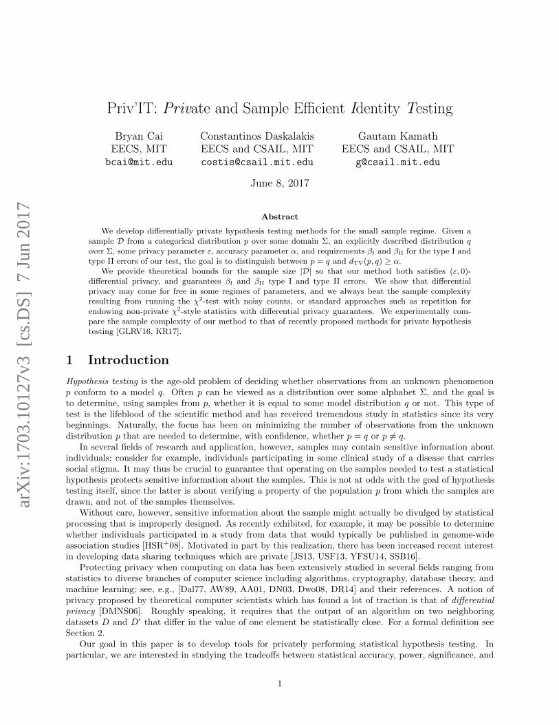
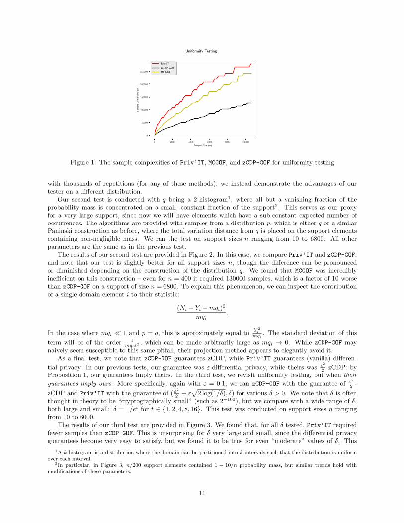
The results of our first test are provided in Figure 1. The x-axis indicates the support size, and the y-axisindicates the minimum number of samples required. We plot three lines, which demonstrate the empiricalnumber of samples required to obtain 1/3 type I and type II error for the different algorithms. We can seethat in this case, zCDP-GOF is the most statistically efficient, followed by MCGOF and Priv’IT.

To explain this difference in statistical efficiency, we note that the theoretical guarantees of Priv’IT

imply that it performs well even when data is sparsely sampled. More precisely, one of the benefits of ourtester is that it can reduce the variance induced by elements whose expected number of occurrences is lessthan 1. Since none of these testers reach this regime (i.e., even zCDP-GOF at n = 10000 expects to see eachelement 10 times), we do not reap the benefits of Priv’IT. Ideally, we would run these algorithms on theuniform distribution at sufficiently large support sizes. However, since this is prohibitively expensive to do

10

0 2000 4000 6000 8000 10000

Support Size (n)

0

50000

100000

150000

200000

250000

Sa

mp

leC

om

ple

xity

(m)

Priv’IT

zCDP-GOF

MCGOF

Uniformity Testing

Figure 1: The sample complexities of Priv’IT, MCGOF, and zCDP-GOF for uniformity testing

with thousands of repetitions (for any of these methods), we instead demonstrate the advantages of ourtester on a different distribution.

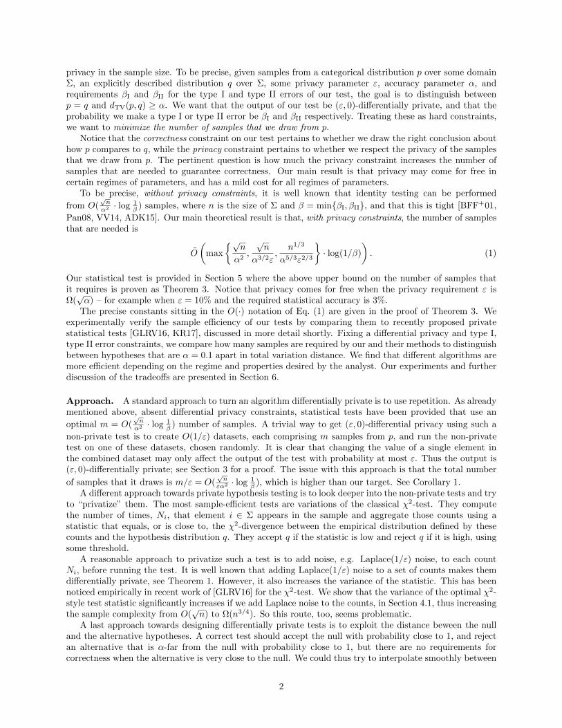
Our second test is conducted with q being a 2-histogram1, where all but a vanishing fraction of theprobability mass is concentrated on a small, constant fraction of the support2. This serves as our proxyfor a very large support, since now we will have elements which have a sub-constant expected number ofoccurrences. The algorithms are provided with samples from a distribution p, which is either q or a similarPaninski construction as before, where the total variation distance from q is placed on the support elementscontaining non-negligible mass. We ran the test on support sizes n ranging from 10 to 6800. All otherparameters are the same as in the previous test.

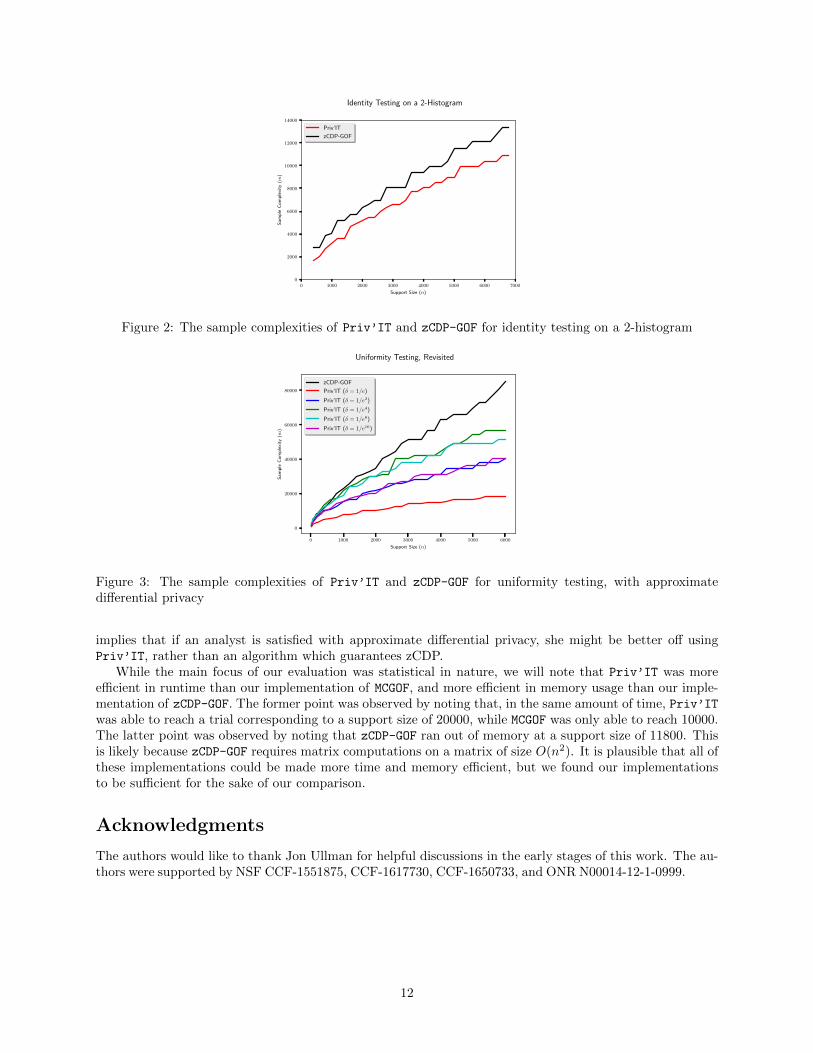
The results of our second test are provided in Figure 2. In this case, we compare Priv’IT and zCDP-GOF,and note that our test is slightly better for all support sizes n, though the difference can be pronouncedor diminished depending on the construction of the distribution q. We found that MCGOF was incrediblyinefficient on this construction – even for n = 400 it required 130000 samples, which is a factor of 10 worsethan zCDP-GOF on a support of size n = 6800. To explain this phenomenon, we can inspect the contributionof a single domain element i to their statistic:

(Ni + Yi −mqi)2

mqi.

In the case where mqi 1 and p = q, this is approximately equal toY 2i

mqi. The standard deviation of this

term will be of the order 1mqiε2

, which can be made arbitrarily large as mqi → 0. While zCDP-GOF maynaively seem susceptible to this same pitfall, their projection method appears to elegantly avoid it.

As a final test, we note that zCDP-GOF guarantees zCDP, while Priv’IT guarantees (vanilla) differen-

tial privacy. In our previous tests, our guarantee was ε-differential privacy, while theirs was ε2

2 -zCDP: byProposition 1, our guarantees imply theirs. In the third test, we revisit uniformity testing, but when their

guarantees imply ours. More specifically, again with ε = 0.1, we ran zCDP-GOF with the guarantee of ε2

2 -

zCDP and Priv’IT with the guarantee of ( ε2

2 + ε√

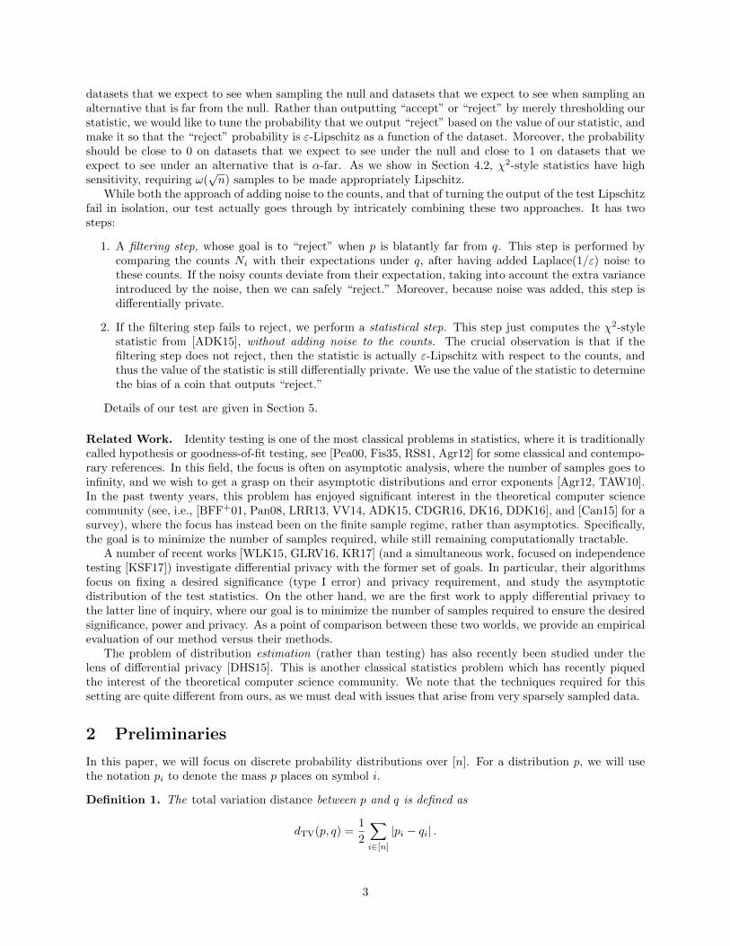
2 log(1/δ), δ) for various δ > 0. We note that δ is oftenthought in theory to be “cryptographically small” (such as 2−100), but we compare with a wide range of δ,both large and small: δ = 1/et for t ∈ 1, 2, 4, 8, 16. This test was conducted on support sizes n rangingfrom 10 to 6000.

The results of our third test are provided in Figure 3. We found that, for all δ tested, Priv’IT requiredfewer samples than zCDP-GOF. This is unsurprising for δ very large and small, since the differential privacyguarantees become very easy to satisfy, but we found it to be true for even “moderate” values of δ. This

1A k-histogram is a distribution where the domain can be partitioned into k intervals such that the distribution is uniformover each interval.

2In particular, in Figure 3, n/200 support elements contained 1 − 10/n probability mass, but similar trends hold withmodifications of these parameters.

11

0 1000 2000 3000 4000 5000 6000 7000

Support Size (n)

0

2000

4000

6000

8000

10000

12000

14000

Sa

mp

leC

om

ple

xity

(m)

Priv’IT

zCDP-GOF

Identity Testing on a 2-Histogram

Figure 2: The sample complexities of Priv’IT and zCDP-GOF for identity testing on a 2-histogram

0 1000 2000 3000 4000 5000 6000

Support Size (n)

0

20000

40000

60000

80000

Sa

mp

leC

om

ple

xity

(m)

zCDP-GOF

Priv’IT (δ = 1/e)

Priv’IT (δ = 1/e2)

Priv’IT (δ = 1/e4)

Priv’IT (δ = 1/e8)

Priv’IT (δ = 1/e16)

Uniformity Testing, Revisited

Figure 3: The sample complexities of Priv’IT and zCDP-GOF for uniformity testing, with approximatedifferential privacy

implies that if an analyst is satisfied with approximate differential privacy, she might be better off usingPriv’IT, rather than an algorithm which guarantees zCDP.

While the main focus of our evaluation was statistical in nature, we will note that Priv’IT was moreefficient in runtime than our implementation of MCGOF, and more efficient in memory usage than our imple-mentation of zCDP-GOF. The former point was observed by noting that, in the same amount of time, Priv’ITwas able to reach a trial corresponding to a support size of 20000, while MCGOF was only able to reach 10000.The latter point was observed by noting that zCDP-GOF ran out of memory at a support size of 11800. Thisis likely because zCDP-GOF requires matrix computations on a matrix of size O(n2). It is plausible that all ofthese implementations could be made more time and memory efficient, but we found our implementationsto be sufficient for the sake of our comparison.

Acknowledgments

The authors would like to thank Jon Ullman for helpful discussions in the early stages of this work. The au-thors were supported by NSF CCF-1551875, CCF-1617730, CCF-1650733, and ONR N00014-12-1-0999.

12

References

[AA01] Dakshi Agrawal and Charu C. Aggarwal. On the design and quantification of privacy preservingdata mining algorithms. In Proceedings of the 20th ACM SIGMOD-SIGACT-SIGART Sympo-sium on Principles of Database Systems, PODS ’01, pages 247–255, New York, NY, USA, 2001.ACM.

[ADK15] Jayadev Acharya, Constantinos Daskalakis, and Gautam Kamath. Optimal testing for propertiesof distributions. In Advances in Neural Information Processing Systems 28, NIPS ’15, pages3577–3598. Curran Associates, Inc., 2015.

[Agr12] Alan Agresti. Categorical Data Analysis. Wiley, 2012.

[AW89] Nabil R. Adam and John C. Worthmann. Security-control methods for statistical databases: Acomparative study. ACM Computing Surveys (CSUR), 21(4):515–556, 1989.

[BFF+01] Tugkan Batu, Eldar Fischer, Lance Fortnow, Ravi Kumar, Ronitt Rubinfeld, and Patrick White.Testing random variables for independence and identity. In Proceedings of the 42nd Annual IEEESymposium on Foundations of Computer Science, FOCS ’01, pages 442–451, Washington, DC,USA, 2001. IEEE Computer Society.

[BS16] Mark Bun and Thomas Steinke. Concentrated differential privacy: Simplifications, extensions,and lower bounds. In Proceedings of the 14th Conference on Theory of Cryptography, TCC ’16-B,pages 635–658, Berlin, Heidelberg, 2016. Springer.

[Can15] Clement L. Canonne. A survey on distribution testing: Your data is big. but is it blue? ElectronicColloquium on Computational Complexity (ECCC), 22(63), 2015.

[Can17] Clement L. Canonne. A short note on Poisson tail bounds. http://www.cs.columbia.edu/

~ccanonne/files/misc/2017-poissonconcentration.pdf, 2017.

[CDGR16] Clement L. Canonne, Ilias Diakonikolas, Themis Gouleakis, and Ronitt Rubinfeld. Testing shaperestrictions of discrete distributions. In Proceedings of the 33rd Symposium on Theoretical Aspectsof Computer Science, STACS ’16, pages 25:1–25:14, 2016.

[Dal77] Tore Dalenius. Towards a methodology for statistical disclosure control. Statistisk Tidskrift,15:429–444, 1977.

[DDK16] Constantinos Daskalakis, Nishanth Dikkala, and Gautam Kamath. Testing Ising models. arXivpreprint arXiv:1612.03147, 2016.

[DHS15] Ilias Diakonikolas, Moritz Hardt, and Ludwig Schmidt. Differentially private learning of struc-tured discrete distributions. In Advances in Neural Information Processing Systems 28, NIPS’15, pages 2566–2574. Curran Associates, Inc., 2015.

[DK16] Ilias Diakonikolas and Daniel M. Kane. A new approach for testing properties of discrete dis-tributions. In Proceedings of the 57th Annual IEEE Symposium on Foundations of ComputerScience, FOCS ’16, pages 685–694, Washington, DC, USA, 2016. IEEE Computer Society.

[DMNS06] Cynthia Dwork, Frank McSherry, Kobbi Nissim, and Adam Smith. Calibrating noise to sensitivityin private data analysis. In Proceedings of the 3rd Conference on Theory of Cryptography, TCC’06, pages 265–284, Berlin, Heidelberg, 2006. Springer.

[DN03] Irit Dinur and Kobbi Nissim. Revealing information while preserving privacy. In Proceedingsof the 22nd ACM SIGMOD-SIGACT-SIGART Symposium on Principles of Database Systems,PODS ’03, pages 202–210, New York, NY, USA, 2003. ACM.

[DR14] Cynthia Dwork and Aaron Roth. The Algorithmic Foundations of Differential Privacy. NowPublishers, Inc., 2014.

13

[Dwo08] Cynthia Dwork. Differential privacy: A survey of results. In Proceedings of the 5th InternationalConference on Theory and Applications of Models of Computation, TAMC ’08, pages 1–19, Berlin,Heidelberg, 2008. Springer.

[Fis35] Ronald A. Fisher. The Design of Experiments. Macmillan, 1935.

[GLRV16] Marco Gaboardi, Hyun-Woo Lim, Ryan M. Rogers, and Salil P. Vadhan. Differentially privatechi-squared hypothesis testing: Goodness of fit and independence testing. In Proceedings of the33rd International Conference on Machine Learning, ICML ’16, pages 1395–1403. JMLR, Inc.,2016.

[HSR+08] Nils Homer, Szabolcs Szelinger, Margot Redman, David Duggan, Waibhav Tembe, Jill Muehling,John V. Pearson, Dietrich A. Stephan, Stanley F. Nelson, and David W. Craig. Resolvingindividuals contributing trace amounts of dna to highly complex mixtures using high-density snpgenotyping microarrays. PLoS Genetics, 4(8):1–9, 2008.

[JS13] Aaron Johnson and Vitaly Shmatikov. Privacy-preserving data exploration in genome-wide asso-ciation studies. In Proceedings of the 19th ACM SIGKDD International Conference on KnowledgeDiscovery and Data Mining, KDD ’13, pages 1079–1087, New York, NY, USA, 2013. ACM.

[Kla00] Bernhard Klar. Bounds on tail probabilities of discrete distributions. Probability in the Engi-neering and Informational Sciences, 14(02):161–171, 2000.

[KR17] Daniel Kifer and Ryan M. Rogers. A new class of private chi-square tests. In Proceedings ofthe 20th International Conference on Artificial Intelligence and Statistics, AISTATS ’17, pages991–1000. JMLR, Inc., 2017.

[KSF17] Kazuya Kakizaki, Jun Sakuma, and Kazuto Fukuchi. Differentially private chi-squared test byunit circle mechanism. In Proceedings of the 34th International Conference on Machine Learning,ICML ’17. JMLR, Inc., 2017.

[LRR13] Reut Levi, Dana Ron, and Ronitt Rubinfeld. Testing properties of collections of distributions.Theory of Computing, 9(8):295–347, 2013.

[Pan08] Liam Paninski. A coincidence-based test for uniformity given very sparsely sampled discretedata. IEEE Transactions on Information Theory, 54(10):4750–4755, 2008.

[Pea00] Karl Pearson. On the criterion that a given system of deviations from the probable in the caseof a correlated system of variables is such that it can be reasonably supposed to have arisen fromrandom sampling. Philosophical Magazine Series 5, 50(302):157–175, 1900.

[Pol15] David Pollard. A few good inequalities. http://www.stat.yale.edu/~pollard/Books/Mini/

Basic.pdf, 2015.

[RS81] Jon N.K. Rao and Alastair J. Scott. The analysis of categorical data from complex samplesurveys: Chi-squared tests for goodness of fit and independence in two-way tables. Journal ofthe Americal Statistical Association, 76(374):221–230, 1981.

[SSB16] Sean Simmons, Cenk Sahinalp, and Bonnie Berger. Enabling privacy-preserving gwass in het-erogeneous human populations. Cell Systems, 3(1):54–61, 2016.

[TAW10] Vincent Y.F. Tan, Animashree Anandkumar, and Alan S. Willsky. Error exponents for compositehypothesis testing of Markov forest distributions. In Proceedings of the 2010 IEEE InternationalSymposium on Information Theory, ISIT ’10, pages 1613–1617, Washington, DC, USA, 2010.IEEE Computer Society.

[USF13] Caroline Uhler, Aleksandra Slavkovic, and Stephen E. Fienberg. Privacy-preserving data sharingfor genome-wide association studies. The Journal of Privacy and Confidentiality, 5(1):137–166,2013.

14

[VV14] Gregory Valiant and Paul Valiant. An automatic inequality prover and instance optimal identitytesting. In Proceedings of the 55th Annual IEEE Symposium on Foundations of Computer Science,FOCS ’14, pages 51–60, Washington, DC, USA, 2014. IEEE Computer Society.

[WLK15] Yue Wang, Jaewoo Lee, and Daniel Kifer. Differentially private hypothesis testing, revisited.arXiv preprint arXiv:1511.03376, 2015.

[YFSU14] Fei Yu, Stephen E. Fienberg, Aleksandra B. Slavkovic, and Caroline Uhler. Scalable privacy-preserving data sharing methodology for genome-wide association studies. Journal of BiomedicalInformatics, 50:133–141, 2014.

15