First-Order Low-Pass Filter - Princeton University
27
Filters, Cost Functions, and Controller Structures Robert Stengel Optimal Control and Estimation MAE 546 Princeton University, 2018 Copyright 2018 by Robert Stengel. All rights reserved. For educational use only. http://www.princeton.edu/~stengel/MAE546.html http://www.princeton.edu/~stengel/OptConEst.html min Δu J = min Δu 1 2 Δx T (t )QΔx(t ) + Δu T (t )RΔu(t ) ⎡ ⎣ ⎤ ⎦ dt 0 ∞ ∫ subject to Δ ! x(t ) = FΔx(t ) + GΔu(t ) ! Dynamic systems as low-pass filters ! Frequency response of dynamic systems ! Shaping system response ! LQ regulators with output vector cost functions ! Implicit model-following ! Cost functions with augmented state vector 1 First-Order Low-Pass Filter 2
Transcript of First-Order Low-Pass Filter - Princeton University
Filters, Cost Functions, and Controller Structures
Robert Stengel Optimal Control and Estimation MAE 546
Princeton University, 2018
Copyright 2018 by Robert Stengel. All rights reserved. For educational use only.http://www.princeton.edu/~stengel/MAE546.html
http://www.princeton.edu/~stengel/OptConEst.html
minΔu
J = minΔu
12
ΔxT (t)QΔx(t)+ ΔuT (t)RΔu(t)⎡⎣ ⎤⎦dt0
∞
∫subject to
Δ!x(t) = FΔx(t)+GΔu(t)
! Dynamic systems as low-pass filters! Frequency response of dynamic systems! Shaping system response
! LQ regulators with output vector cost functions! Implicit model-following! Cost functions with augmented state vector
1
First-Order Low-Pass Filter
2
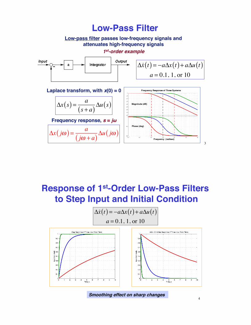
Low-Pass FilterLow-pass filter passes low-frequency signals and
attenuates high-frequency signals1st-order example
Δ!x t( ) = −aΔx t( ) + aΔu t( )a = 0.1, 1, or 10
Δx s( ) = as + a( )Δu s( )
Δx jω( ) = ajω + a( )Δu jω( )
Laplace transform, with x(0) = 0
Frequency response, s = jω
3
Response of 1st-Order Low-Pass Filters to Step Input and Initial Condition
Δ!x t( ) = −aΔx t( ) + aΔu t( )a = 0.1, 1, or 10
Smoothing effect on sharp changes4
Frequency Response of Dynamic Systems
5
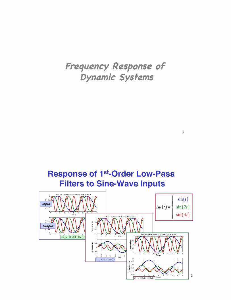
Response of 1st-Order Low-Pass Filters to Sine-Wave Inputs
Δu t( ) =sin t( )sin 2t( )sin 4t( )
⎧
⎨⎪⎪
⎩⎪⎪
!x t( ) = −x t( ) + u t( )
x t( ) = −10x t( ) +10u t( )
x t( ) = −0.1x t( ) + 0.1u t( )
Input
Output
6
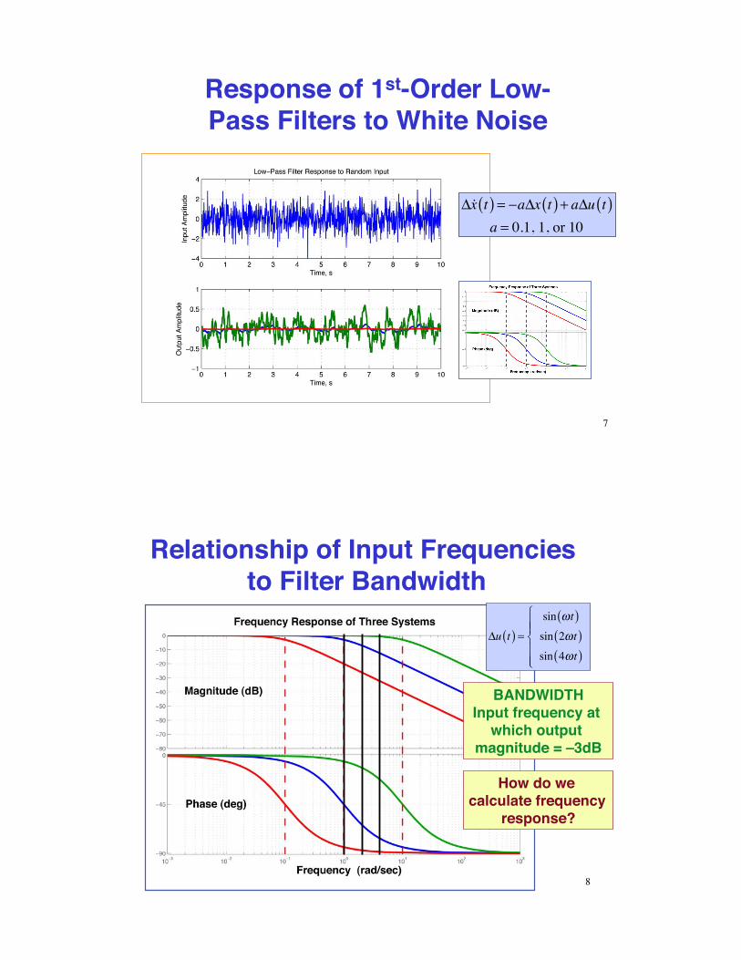
Response of 1st-Order Low-Pass Filters to White Noise
Δ!x t( ) = −aΔx t( ) + aΔu t( )a = 0.1, 1, or 10
7
Relationship of Input Frequencies to Filter Bandwidth
Δu t( ) =sin ωt( )sin 2ωt( )sin 4ωt( )
⎧
⎨⎪⎪
⎩⎪⎪
How do we calculate frequency
response?
BANDWIDTHInput frequency at
which output magnitude = –3dB
8
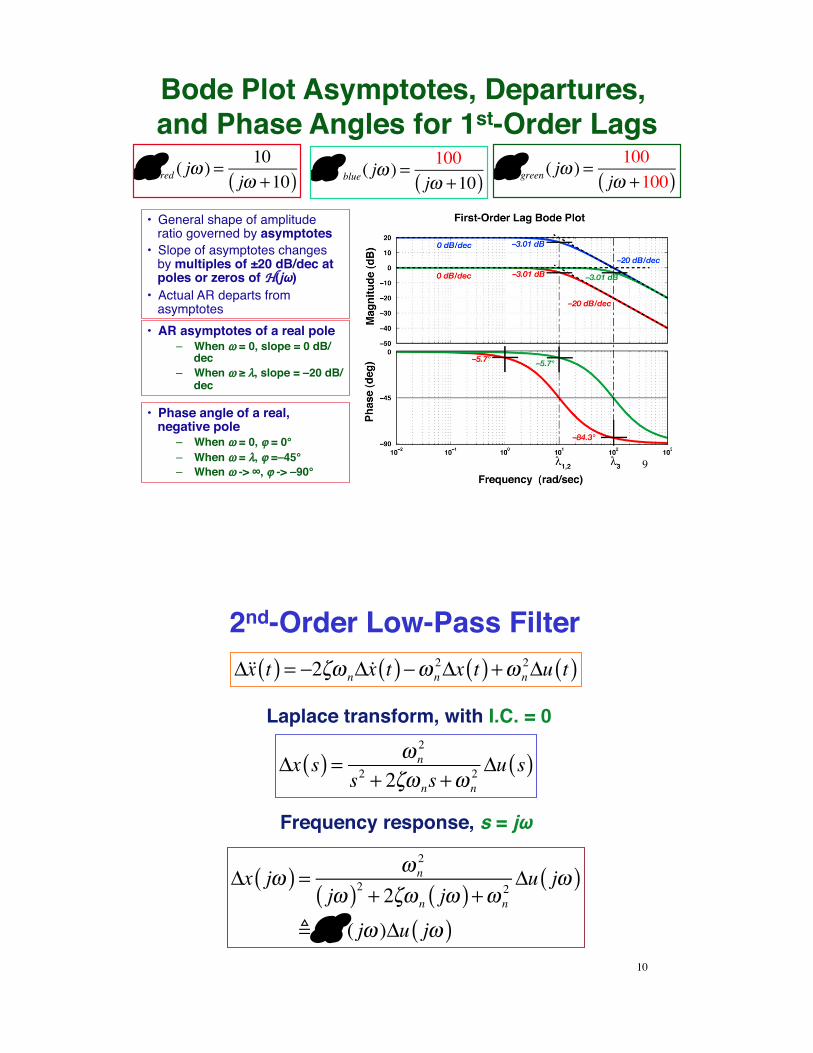
Bode Plot Asymptotes, Departures, and Phase Angles for 1st-Order Lags
• General shape of amplitude ratio governed by asymptotes
• Slope of asymptotes changes by multiples of ±20 dB/dec at poles or zeros of H(jω)
• Actual AR departs from asymptotes
• Phase angle of a real, negative pole
– When ω = 0, ϕ = 0°– When ω = λ, ϕ =–45°– When ω -> ∞, ϕ -> –90°
• AR asymptotes of a real pole– When ω = 0, slope = 0 dB/
dec– When ω ≥ λ, slope = –20 dB/
dec
9
H red ( jω ) =
10jω +10( )
H blue( jω ) =100jω +10( )
H green ( jω ) =100
jω +100( )
2nd-Order Low-Pass Filter
Δ!!x t( ) = −2ζω nΔ!x t( )−ω n2Δx t( ) +ω n
2Δu t( )
Laplace transform, with I.C. = 0
Frequency response, s = jω
Δx s( ) = ω n2
s2 + 2ζω ns +ω n2 Δu s( )
Δx jω( ) = ω n2
jω( )2 + 2ζω n jω( ) +ω n2Δu jω( )
!H ( jω )Δu jω( )10
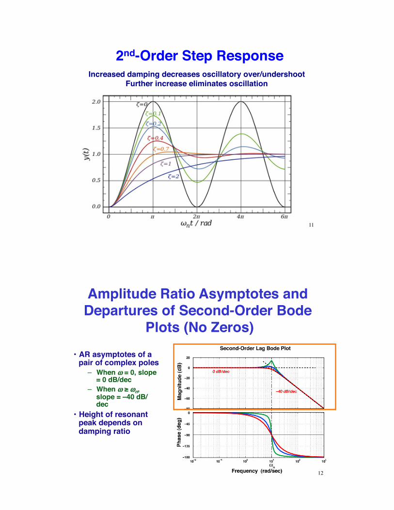
2nd-Order Step Response
11
Increased damping decreases oscillatory over/undershootFurther increase eliminates oscillation
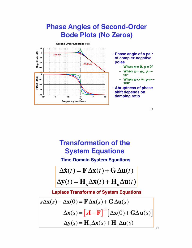
Amplitude Ratio Asymptotes and Departures of Second-Order Bode
Plots (No Zeros)• AR asymptotes of a
pair of complex poles– When ω = 0, slope
= 0 dB/dec– When ω ≥ ωn,
slope = –40 dB/dec
• Height of resonant peak depends on damping ratio
12
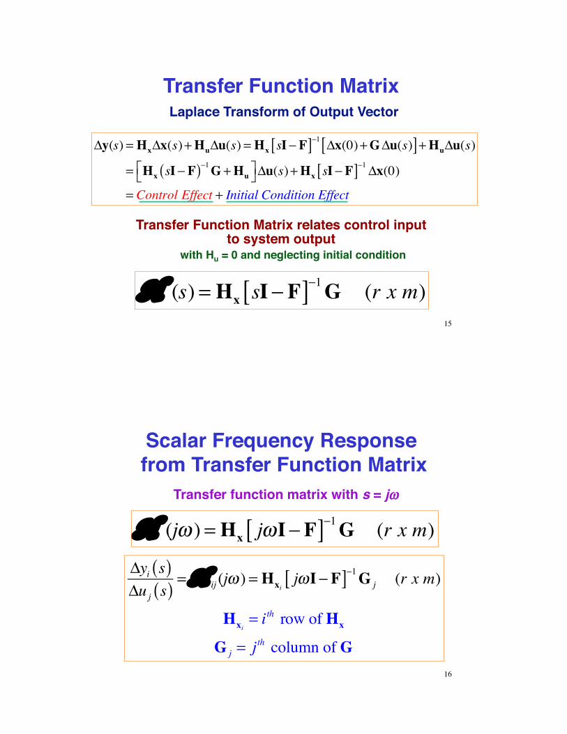
Phase Angles of Second-Order Bode Plots (No Zeros)
• Phase angle of a pair of complex negative poles
– When ω = 0, ϕ = 0°– When ω = ωn, ϕ =–
90°– When ω -> ∞, ϕ -> –
180°• Abruptness of phase
shift depends on damping ratio
13
Δ!x(t) = FΔx(t)+GΔu(t)Δy(t) = HxΔx(t)+HuΔu(t)
Time-Domain System Equations
Laplace Transforms of System Equations
sΔx(s)− Δx(0) = FΔx(s)+GΔu(s)
Δx(s) = sI− F[ ]−1 Δx(0)+GΔu(s)[ ]Δy(s) = HxΔx(s)+HuΔu(s)
Transformation of the System Equations
14
Transfer Function Matrix
Transfer Function Matrix relates control input to system output
with Hu = 0 and neglecting initial condition
H (s) = Hx sI− F[ ]−1G (r x m)
Laplace Transform of Output Vector
Δy(s) = HxΔx(s)+HuΔu(s) = Hx sI− F[ ]−1 Δx(0)+GΔu(s)[ ]+HuΔu(s)
= Hx sI− F( )−1G +Hu⎡⎣ ⎤⎦Δu(s)+Hx sI− F[ ]−1Δx(0)
= Control Effect + Initial Condition Effect
15
Scalar Frequency Response from Transfer Function Matrix
Transfer function matrix with s = jω
H (jω ) = Hx jωI− F[ ]−1G (r x m)
Δyi s( )Δuj s( ) = H ij (jω ) = Hxi
jωI− F[ ]−1G j (r x m)
Hxi= ith row of Hx
G j = j th column of G16
Second-Order Transfer Function
H (s) = HxA s( )G =h11 h12h21 h22
⎡
⎣⎢⎢
⎤
⎦⎥⎥
adjs − f11( ) − f12− f21 s − f22( )
⎡
⎣
⎢⎢
⎤
⎦
⎥⎥
dets − f11( ) − f12− f21 s − f22( )
⎛
⎝⎜⎜
⎞
⎠⎟⎟
g11 g12g21 f22
⎡
⎣⎢⎢
⎤
⎦⎥⎥
(n = m = r = 2)
Second-order transfer function matrix
r × n( ) n × n( ) n × m( )= r × m( ) = 2 × 2( )
Δ!x t( ) =Δ!x1 t( )Δ!x2 t( )
⎡
⎣⎢⎢
⎤
⎦⎥⎥=
f11 f12f21 f22
⎡
⎣⎢⎢
⎤
⎦⎥⎥
Δx1 t( )Δx2 t( )
⎡
⎣⎢⎢
⎤
⎦⎥⎥+
g11 g12g21 f22
⎡
⎣⎢⎢
⎤
⎦⎥⎥
Δu1 t( )Δu2 t( )
⎡
⎣⎢⎢
⎤
⎦⎥⎥
Δy t( ) =Δy1 t( )Δy2 t( )
⎡
⎣⎢⎢
⎤
⎦⎥⎥=
h11 h12h21 h22
⎡
⎣⎢⎢
⎤
⎦⎥⎥
Δx1 t( )Δx2 t( )
⎡
⎣⎢⎢
⎤
⎦⎥⎥
Second-order dynamic system
17
Scalar Transfer Function from Δuj to Δyi
H ij (s) =
kijnij (s)Δ(s)
=kij s
q + bq−1sq−1 + ...+ b1s + b0( )
sn + an−1sn−1 + ...+ a1s + a0( )
# zeros = q# poles = n
Just one element of the matrix, H(s)Denominator polynomial contains n roots
Each numerator term is a polynomial with q zeros, where q varies from term to term and ≤ n – 1
=kij s− z1( )ij s− z2( )ij ... s− zq( )ij
s−λ1( ) s−λ2( )... s−λn( )18
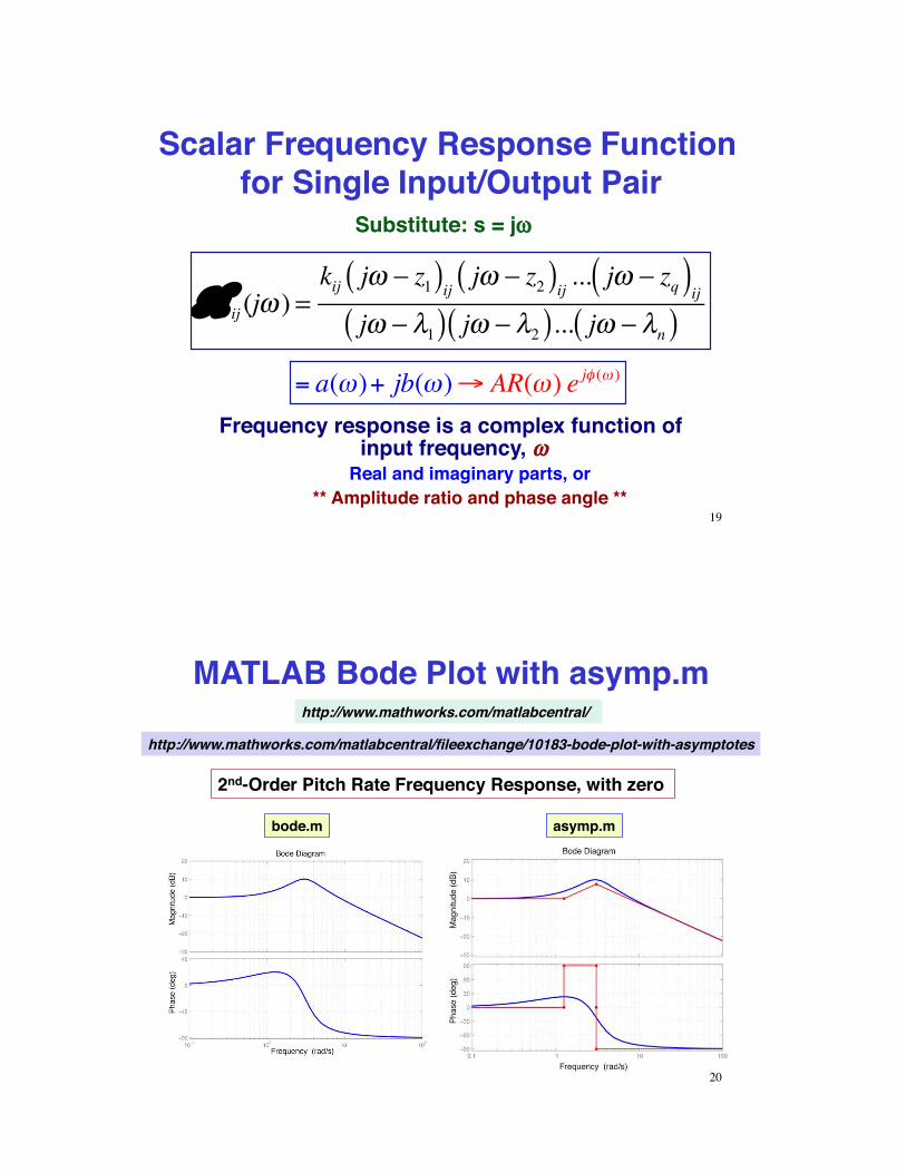
Scalar Frequency Response Function for Single Input/Output Pair
H ij (jω ) =
kij jω − z1( )ij jω − z2( )ij ... jω − zq( )ijjω − λ1( ) jω − λ2( )... jω − λn( )
Substitute: s = jω
Frequency response is a complex function of input frequency, ω
Real and imaginary parts, or** Amplitude ratio and phase angle **
= a(ω)+ jb(ω)→ AR(ω) e jφ (ω )
19
MATLAB Bode Plot with asymp.mhttp://www.mathworks.com/matlabcentral/
http://www.mathworks.com/matlabcentral/fileexchange/10183-bode-plot-with-asymptotes
2nd-Order Pitch Rate Frequency Response, with zero
asymp.mbode.m
20
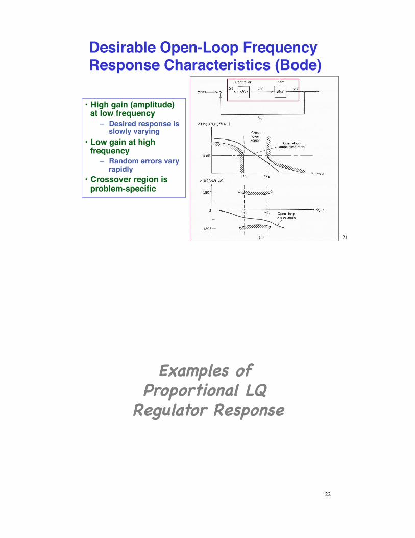
• High gain (amplitude) at low frequency
– Desired response is slowly varying
• Low gain at high frequency
– Random errors vary rapidly
• Crossover region is problem-specific
Desirable Open-Loop Frequency Response Characteristics (Bode)
21
Examples of Proportional LQ
Regulator Response
22
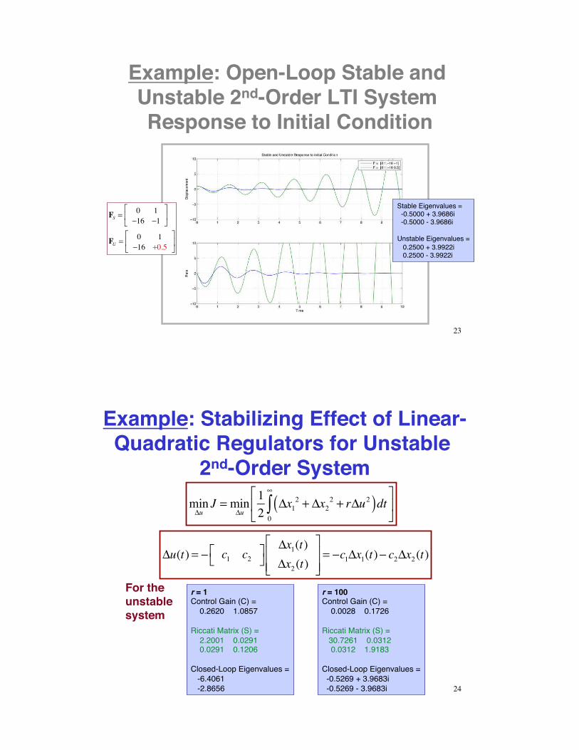
Example: Open-Loop Stable and Unstable 2nd-Order LTI System Response to Initial Condition
Stable Eigenvalues = -0.5000 + 3.9686i -0.5000 - 3.9686i
Unstable Eigenvalues = 0.2500 + 3.9922i 0.2500 - 3.9922i
FS =0 1
−16 −1⎡
⎣⎢
⎤
⎦⎥
FU = 0 1−16 +0.5
⎡
⎣⎢
⎤
⎦⎥
23
Example: Stabilizing Effect of Linear-Quadratic Regulators for Unstable
2nd-Order System
r = 1Control Gain (C) = 0.2620 1.0857
Riccati Matrix (S) = 2.2001 0.0291 0.0291 0.1206
Closed-Loop Eigenvalues = -6.4061 -2.8656
r = 100Control Gain (C) = 0.0028 0.1726
Riccati Matrix (S) = 30.7261 0.0312 0.0312 1.9183
Closed-Loop Eigenvalues = -0.5269 + 3.9683i -0.5269 - 3.9683i
minΔu
J = minΔu
12
Δx12 + Δx2
2 + rΔu2( )dt0
∞
∫⎡
⎣⎢
⎤
⎦⎥
Δu(t) = − c1 c2⎡⎣
⎤⎦
Δx1(t)Δx2 (t)
⎡
⎣⎢⎢
⎤
⎦⎥⎥= −c1Δx1(t)− c2Δx2 (t)
For the unstable system
24
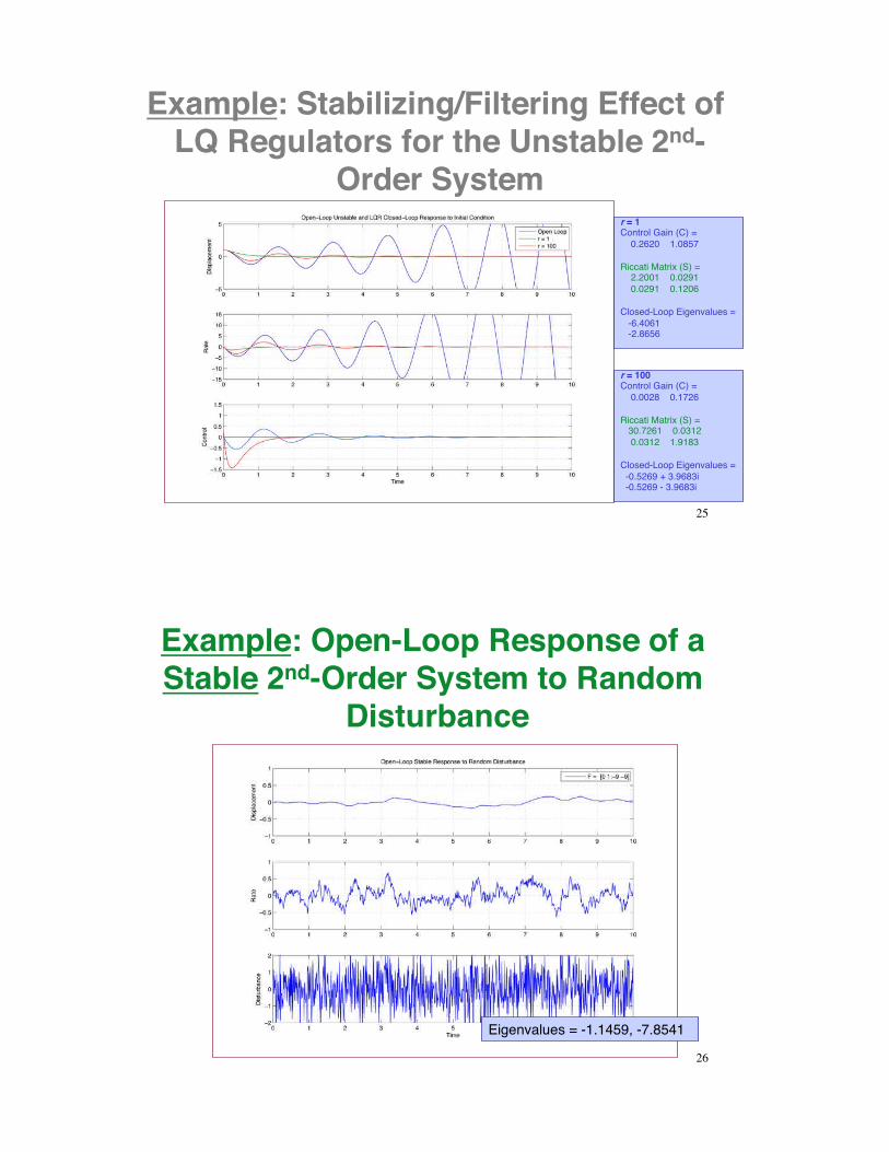
Example: Stabilizing/Filtering Effect of LQ Regulators for the Unstable 2nd-
Order Systemr = 1Control Gain (C) = 0.2620 1.0857
Riccati Matrix (S) = 2.2001 0.0291 0.0291 0.1206
Closed-Loop Eigenvalues = -6.4061 -2.8656
r = 100Control Gain (C) = 0.0028 0.1726
Riccati Matrix (S) = 30.7261 0.0312 0.0312 1.9183
Closed-Loop Eigenvalues = -0.5269 + 3.9683i -0.5269 - 3.9683i
25
Example: Open-Loop Response of a Stable 2nd-Order System to Random
Disturbance
Eigenvalues = -1.1459, -7.8541
26
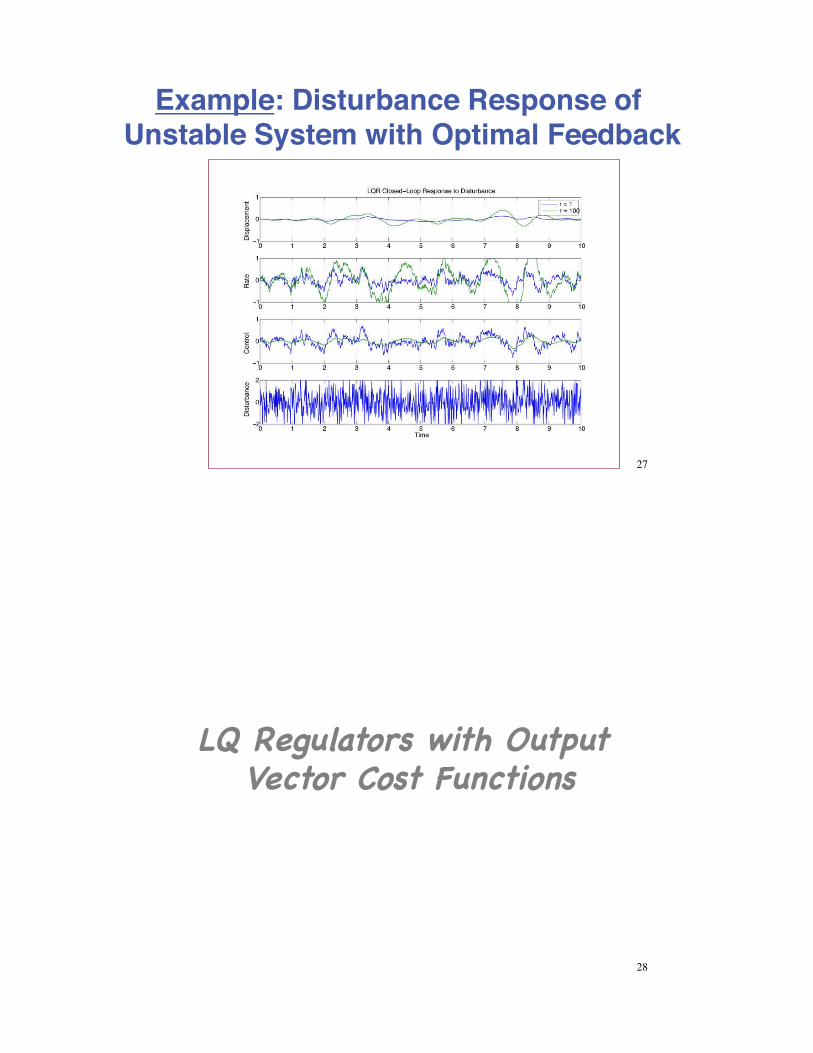
Example: Disturbance Response of Unstable System with Optimal Feedback
27
LQ Regulators with Output Vector Cost Functions
28
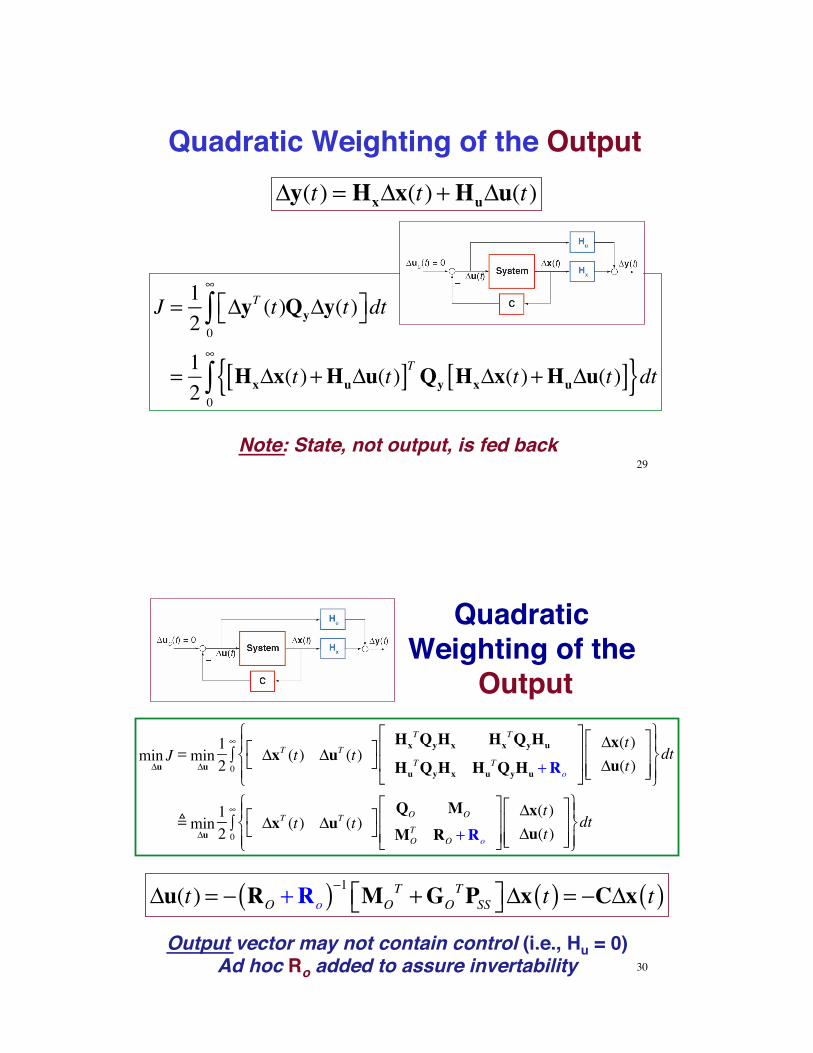
Quadratic Weighting of the Output
J = 12
ΔyT (t)QyΔy(t)⎡⎣ ⎤⎦dt0
∞
∫
= 12
HxΔx(t)+HuΔu(t)[ ]T Qy HxΔx(t)+HuΔu(t)[ ]{ }dt0
∞
∫
Δy(t) = HxΔx(t) +HuΔu(t)
29Note: State, not output, is fed back
Quadratic Weighting of the
Output
Δu(t) = − RO +Ro( )−1 MOT +GO
TPSS⎡⎣ ⎤⎦Δx t( ) = −CΔx t( )
Δumin J =
Δumin
12
ΔxT (t) ΔuT (t)⎡⎣
⎤⎦Hx
TQyHx HxTQyHu
HuTQyHx Hu
TQyHu +Ro
⎡
⎣
⎢⎢
⎤
⎦
⎥⎥
Δx(t)Δu(t)
⎡
⎣⎢⎢
⎤
⎦⎥⎥
⎧⎨⎪
⎩⎪
⎫⎬⎪
⎭⎪dt
0
∞
∫
!Δumin
12
ΔxT (t) ΔuT (t)⎡⎣
⎤⎦QO MO
MOT RO +Ro
⎡
⎣⎢⎢
⎤
⎦⎥⎥
Δx(t)Δu(t)
⎡
⎣⎢⎢
⎤
⎦⎥⎥
⎧⎨⎪
⎩⎪
⎫⎬⎪
⎭⎪dt
0
∞
∫
30
Output vector may not contain control (i.e., Hu = 0)Ad hoc Ro added to assure invertability
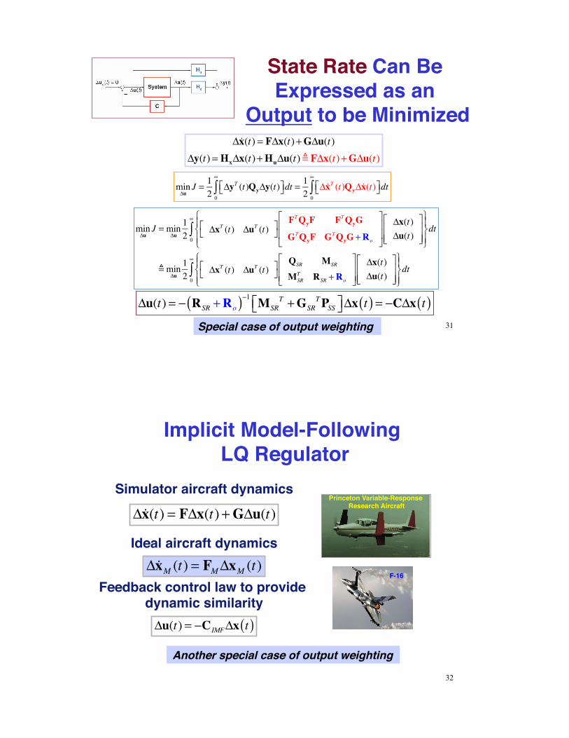
State Rate Can Be Expressed as an
Output to be Minimized
minΔu
J = 12
ΔyT (t)QyΔy(t)⎡⎣ ⎤⎦dt0
∞
∫ = 12
Δ!xT (t)QyΔ!x(t)⎡⎣ ⎤⎦dt0
∞
∫
Δu(t) = − RSR +Ro( )−1 MSRT +GSR
TPSS⎡⎣ ⎤⎦Δx t( ) = −CΔx t( )
Δ!x(t) = FΔx(t)+GΔu(t)Δy(t) = HxΔx(t)+HuΔu(t) " FΔx(t)+GΔu(t)
Special case of output weighting
minΔu
J = minΔu
12
ΔxT (t) ΔuT (t)⎡⎣
⎤⎦FTQyF FTQyG
GTQyF GTQyG +Ro
⎡
⎣
⎢⎢
⎤
⎦
⎥⎥
Δx(t)Δu(t)
⎡
⎣⎢⎢
⎤
⎦⎥⎥
⎧⎨⎪
⎩⎪
⎫⎬⎪
⎭⎪dt
0
∞
∫
! minΔu
12
ΔxT (t) ΔuT (t)⎡⎣
⎤⎦QSR MSR
MSRT RSR +Ro
⎡
⎣⎢⎢
⎤
⎦⎥⎥
Δx(t)Δu(t)
⎡
⎣⎢⎢
⎤
⎦⎥⎥
⎧⎨⎪
⎩⎪
⎫⎬⎪
⎭⎪dt
0
∞
∫
31
Implicit Model-Following LQ Regulator
Δu(t) = −CIMFΔx t( )
Δx(t) = FΔx(t) +GΔu(t)
Simulator aircraft dynamics
ΔxM (t) = FMΔxM (t)Ideal aircraft dynamics
Feedback control law to provide dynamic similarity
Another special case of output weighting32
Princeton Variable-Response Research Aircraft
F-16

Implicit Model-Following LQ Regulator
Assume state dimensions are the sameΔ!x(t) = FΔx(t)+GΔu(t)Δ!xM (t) = FMΔxM (t)
If simulation is successful,ΔxM (t) ≈ Δx(t) and Δ!xM (t) ≈ FMΔx(t)
33
Implicit Model-Following LQ Regulator
J = 1
2Δx(t)− ΔxM (t)[ ]T QM Δx(t)− ΔxM (t)[ ]{ }dt
0
∞
∫
Δu(t) = − R IMF +Ro( )−1 M IMFT +G IMF
TPSS⎡⎣ ⎤⎦Δx t( ) = −CΔx t( )
Cost function penalizes difference between actual and ideal model dynamics
Therefore, ideal model is implicit in the optimizing feedback control law
minΔu
J = minΔu
12
Δx(t) Δu(t)⎡⎣
⎤⎦T F − FM( )T QM F − FM( ) F − FM( )T QMG
GTQM F − FM( ) GTQMG +Ro
⎡
⎣
⎢⎢
⎤
⎦
⎥⎥
Δx(t)Δu(t)
⎡
⎣⎢⎢
⎤
⎦⎥⎥
⎧⎨⎪
⎩⎪
⎫⎬⎪
⎭⎪dt
0
∞
∫
! minΔu
12
Δx(t) Δu(t)⎡⎣
⎤⎦T QIMF M IMF
M IMFT R IMF +Ro
⎡
⎣⎢⎢
⎤
⎦⎥⎥
Δx(t)Δu(t)
⎡
⎣⎢⎢
⎤
⎦⎥⎥
⎧⎨⎪
⎩⎪
⎫⎬⎪
⎭⎪dt
0
∞
∫
34
Cost Functions with Augmented State Vector
35
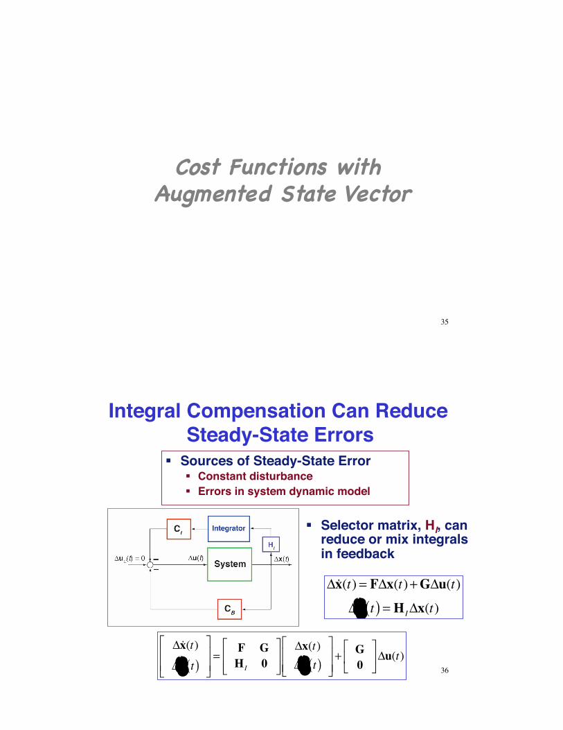
Integral Compensation Can Reduce Steady-State Errors
Δ!x(t) = FΔx(t)+GΔu(t)
Δ!ξ t( ) = H IΔx(t)
! Selector matrix, HI, can reduce or mix integrals in feedback
! Sources of Steady-State Error! Constant disturbance! Errors in system dynamic model
36
Δ!x(t)
Δ!ξ t( )⎡
⎣⎢⎢
⎤
⎦⎥⎥=
F GH I 0
⎡
⎣⎢⎢
⎤
⎦⎥⎥
Δx(t)Δξ t( )
⎡
⎣⎢⎢
⎤
⎦⎥⎥+ G
0⎡
⎣⎢
⎤
⎦⎥Δu(t)
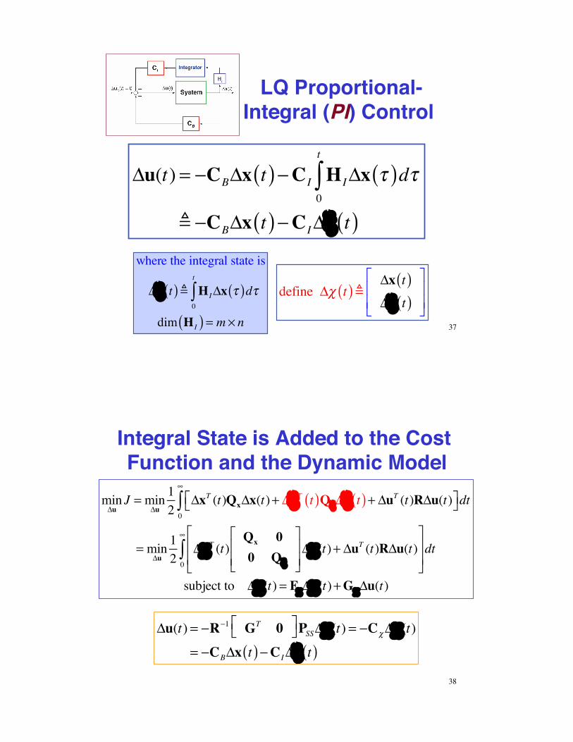
LQ Proportional-Integral (PI) Control
Δu(t) = −CBΔx t( )−CI H IΔx τ( )dτ0
t
∫! −CBΔx t( )−CIΔξ t( )
where the integral state is
Δξ t( ) ! H IΔx τ( )dτ0
t
∫dim H I( ) = m × n
define Δχ t( ) !Δx t( )Δξ t( )
⎡
⎣⎢⎢
⎤
⎦⎥⎥
37
Integral State is Added to the Cost Function and the Dynamic Model
minΔu
J = minΔu
12
ΔxT (t)QxΔx(t)+ ΔξT t( )QξΔξ t( ) + ΔuT (t)RΔu(t)⎡⎣ ⎤⎦dt0
∞
∫
= minΔu
12
ΔχT (t)Qx 00 Qξ
⎡
⎣⎢⎢
⎤
⎦⎥⎥Δχ(t)+ ΔuT (t)RΔu(t)
⎡
⎣
⎢⎢
⎤
⎦
⎥⎥dt
0
∞
∫
subject to Δ!χ(t) = FχΔχ(t)+GχΔu(t)
Δu(t) = −R−1 GT 0⎡⎣ ⎤⎦PSSΔχ(t) = −CχΔχ(t)
= −CBΔx t( )−CIΔξ t( )38
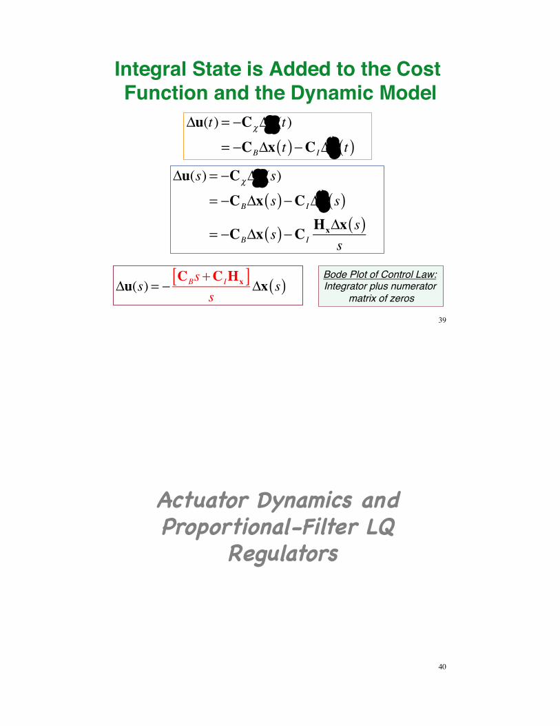
Integral State is Added to the Cost Function and the Dynamic Model
Δu(t) = −CχΔχ(t)
= −CBΔx t( )−CIΔξ t( )Δu(s) = −CχΔχ(s)
= −CBΔx s( )−CIΔξ s( )
= −CBΔx s( )−CIHxΔx s( )
s
Δu(s) = −CBs +CIHx[ ]
sΔx s( )
Bode Plot of Control Law: Integrator plus numerator
matrix of zeros
39
Actuator Dynamics and Proportional-Filter LQ
Regulators
40
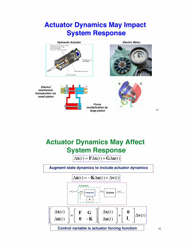
Actuator Dynamics May Impact System Response
41
Force multiplication by
large piston
Electro/mechanical
transduction via small piston
Hydraulic Actuator Electric Motor
Actuator Dynamics May Affect System Response
Δ!x(t)Δ !u(t)
⎡
⎣⎢⎢
⎤
⎦⎥⎥= F G
0 −K⎡
⎣⎢
⎤
⎦⎥
Δx(t)Δu(t)
⎡
⎣⎢⎢
⎤
⎦⎥⎥+
0Iv
⎡
⎣⎢⎢
⎤
⎦⎥⎥Δv(t)
Control variable is actuator forcing function
Augment state dynamics to include actuator dynamics
42
Δ!x(t) = FΔx(t)+GΔu(t)
Δ !u(t) = −KΔu(t)+ Δv(t)
LQ Regulator with Actuator Dynamics
minΔv
J = minΔv
12
ΔxT (t)QxΔx(t)+ ΔuT (t)RuΔu(t)+ ΔvT (t)RvΔv(t)⎡⎣ ⎤⎦dt0
∞
∫
= minΔv
12
ΔχT (t)Qx 00 Ru
⎡
⎣⎢⎢
⎤
⎦⎥⎥Δχ(t)+ ΔvT (t)RvΔv(t)
⎡
⎣⎢⎢
⎤
⎦⎥⎥dt
0
∞
∫
Re-define state and control vectors
Δχ(t) !Δx(t)Δu(t)
⎡
⎣⎢⎢
⎤
⎦⎥⎥; Δv t( ) = Control
Fχ !F G0 −K
⎡
⎣⎢
⎤
⎦⎥; Gχ !
0Iv
⎡
⎣⎢⎢
⎤
⎦⎥⎥
43 subject to Δ!χ(t) = FχΔχ(t)+GχΔv(t)
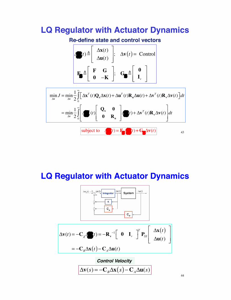
LQ Regulator with Actuator Dynamics
Δv(t) = −CχΔχ(t) = −Rv−1 0 Iv⎡⎣
⎤⎦TPSS
Δx t( )Δu(t)
⎡
⎣⎢⎢
⎤
⎦⎥⎥
= −CBΔx t( )−CAΔu(t)
Δv(s) = −CBΔx s( )−CAΔu(s)44
Control Velocity
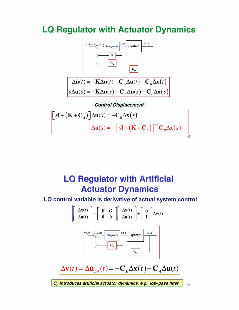
LQ Regulator with Actuator Dynamics
Control Displacement
Δ !u(t) = −KΔu(t)−CAΔu(t)−CBΔx t( )sΔu(s) = −KΔu(s)−CAΔu(s)−CBΔx s( )
sI+ K +CA( )⎡⎣ ⎤⎦Δu(s) = −CBΔx s( )Δu(s) = − sI+ K +CA( )⎡⎣ ⎤⎦
−1CBΔx s( )
45
LQ Regulator with Artificial Actuator Dynamics
Δx(t)Δ u(t)
⎡
⎣⎢⎢
⎤
⎦⎥⎥= F G
0 0⎡
⎣⎢
⎤
⎦⎥
Δx(t)Δu(t)
⎡
⎣⎢⎢
⎤
⎦⎥⎥+ 0
I⎡
⎣⎢
⎤
⎦⎥Δv(t)
Δv(t) = Δ !uInt (t) = −CBΔx t( )−CAΔu(t)
CA introduces artificial actuator dynamics, e.g., low-pass filter
LQ control variable is derivative of actual system control
46
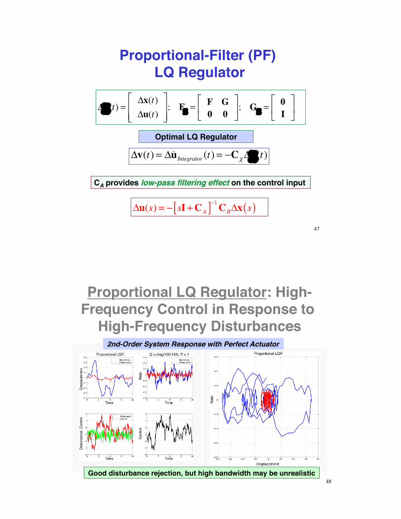
Proportional-Filter (PF) LQ Regulator
Δχ(t) =Δx(t)Δu(t)
⎡
⎣⎢⎢
⎤
⎦⎥⎥; Fχ =
F G0 0
⎡
⎣⎢
⎤
⎦⎥; Gχ =
0I
⎡
⎣⎢
⎤
⎦⎥
Δv(t) = Δ !uIntegrator (t) = −CχΔχ(t)
CA provides low-pass filtering effect on the control input
Δu(s) = − sI+CA[ ]−1CBΔx s( )
Optimal LQ Regulator
47
Proportional LQ Regulator: High-Frequency Control in Response to
High-Frequency Disturbances2nd-Order System Response with Perfect Actuator
Good disturbance rejection, but high bandwidth may be unrealistic48
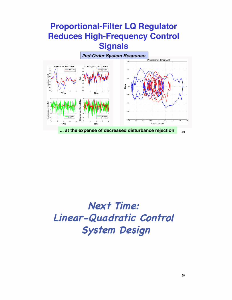
Proportional-Filter LQ Regulator Reduces High-Frequency Control
Signals 2nd-Order System Response
... at the expense of decreased disturbance rejection 49
Next Time: Linear-Quadratic Control
System Design
50
Supplemental Material
51
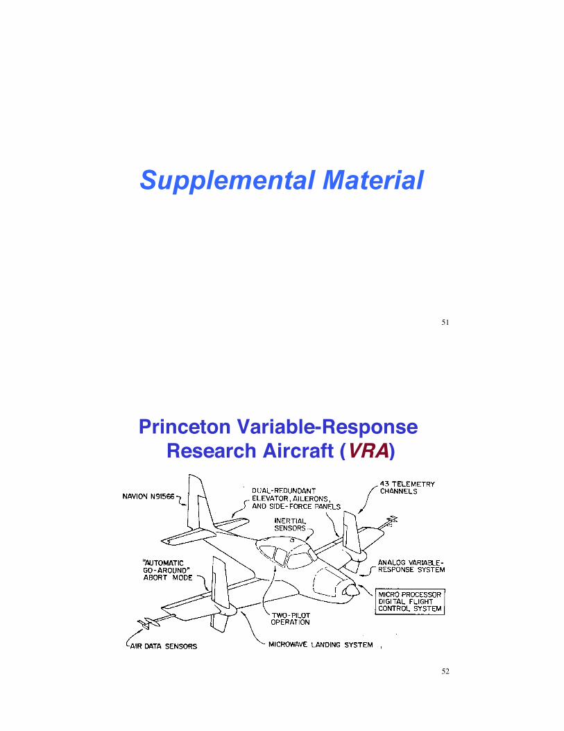
Princeton Variable-Response Research Aircraft (VRA)
52
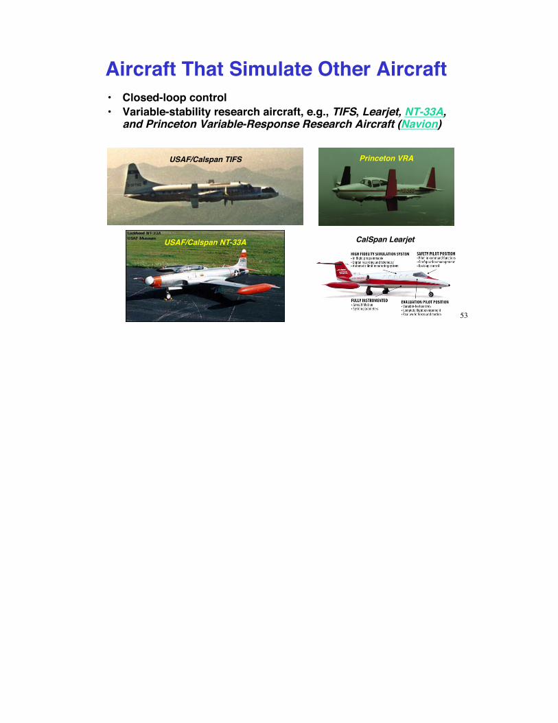
Aircraft That Simulate Other Aircraft• Closed-loop control• Variable-stability research aircraft, e.g., TIFS, Learjet, NT-33A,
and Princeton Variable-Response Research Aircraft (Navion)
USAF/Calspan TIFS
CalSpan Learjet
Princeton VRA
USAF/Calspan NT-33A
53