Extensional Equivalence and Singleton Types

Extensional Equivalence and Singleton Types

CHRISTOPHER A. STONE

Harvey Mudd College

and

ROBERT HARPER

Carnegie Mellon University

In this paper we study a λ-calculus enriched with singleton types, where the type S(M) classifiesall terms of base type provably equivalent to the term M . We also have dependent types for pairs

and functions (Σ and Π) and a sub-kinding relation induced by the observation that any term of

the base type provably equivalent to M is in fact a term of the base type. The decidability oftype checking for this language is non-obvious, since to type check we need to determine whether

two well-formed terms are equivalent. But in the presence of singleton types, the provability ofan equivalence judgment Γ ` M1 ≡ M2 : A can depend both on singletons within the typingcontext Γ and on the particular kind A at which the type constructors M1 and M2 are compared.

Thus, standard context-insensitive rewriting methods are not directly applicable.In this paper we define the λΠΣS

≤ calculus. We prove decidability of term equivalence for

λΠΣS≤ by exhibiting a novel kind-directed algorithm for directly computing normal forms. The

correctness of this normalization algorithm is proved using an unusual variant of Kripke logicalrelations organized around sets; rather than defining a logical equivalence relation, we work directlywith (subsets of) the corresponding equivalence classes.

Finally, we use the results for normalization to show the decidability of well-formedness forterms and types, as well as the correctness of a more efficient direct comparison algorithm for

checking equivalence.The λΠΣS

≤ calculus is a model of the constructors and kinds of the intermediate language used

by the TILT compiler for Standard ML. Thus the decidability of λΠΣS≤ term equivalence allows

us to show decidability of type checking for this intermediate language, while the consistency

of equivalence allows us to prove type safety for of the intermediate language. The algorithms

derived here form the core of the type checker used internally for sanity checking within TILT.

Categories and Subject Descriptors: []:

General Terms:

Additional Key Words and Phrases:

1. INTRODUCTION

Lambda calculus models of programming languages are of both theoretical and practical importance. Onthe theory side they support formal reasoning about the language, including type safety and equationalproperties. On the practical side they support certifying compilation through type-directed translationsbetween typed intermediate languages [Tarditi et al. 1996; Morrisett et al. 1997].

Conventional type systems such as Fω go a long way towards modeling programming language constructssuch as polymorphism, but they do not provide an adequate account of type definitions. For example,although it is well-known how to define local definitions (let) in terms of function application, this does notdirectly translate for definitions of type variables. If we have the polymorphic identity id : ∀α.α⇀α then

This research originally started while the first author was at Carnegie Mellon University. It was supported in part by theUS Army Research Office under Grant No. DAAH04-94-G-0289 and in part by the Advanced Research Projects Agency CSTO

under the title “The Fox Project: Advanced Languages for Systems Software”, ARPA Order No. C533, issued by ESC/ENS

under Contract No. F19628-95-C-0050. The views and conclusions contained in this document are those of the authors andshould not be interpreted as representing the official policies, either expressed or implied, of the U.S. Government.

Permission to make digital/hard copy of all or part of this material without fee for personal or classroom use provided thatthe copies are not made or distributed for profit or commercial advantage, the ACM copyright/server notice, the title of thepublication, and its date appear, and notice is given that copying is by permission of the ACM, Inc. To copy otherwise, to

republish, to post on servers, or to redistribute to lists requires prior specific permission and/or a fee.

ACM Transactions on Programming Languages and Systems, Vol. TBD, No. TDB, Month Year, Pages 1–??.

2 · Christopher A. Stone and Robert Harper

the expression

letα = int×int in id[α](3, 4)

seems unobjectionable, whereas the corresponding application

(Λα.id[α](3, 4))[int×int]

is ill-typed because its subterm Λα.id[α](3, 4) is not well-formed.More complex type definitions occur in the Standard ML module language, where we can have a structure

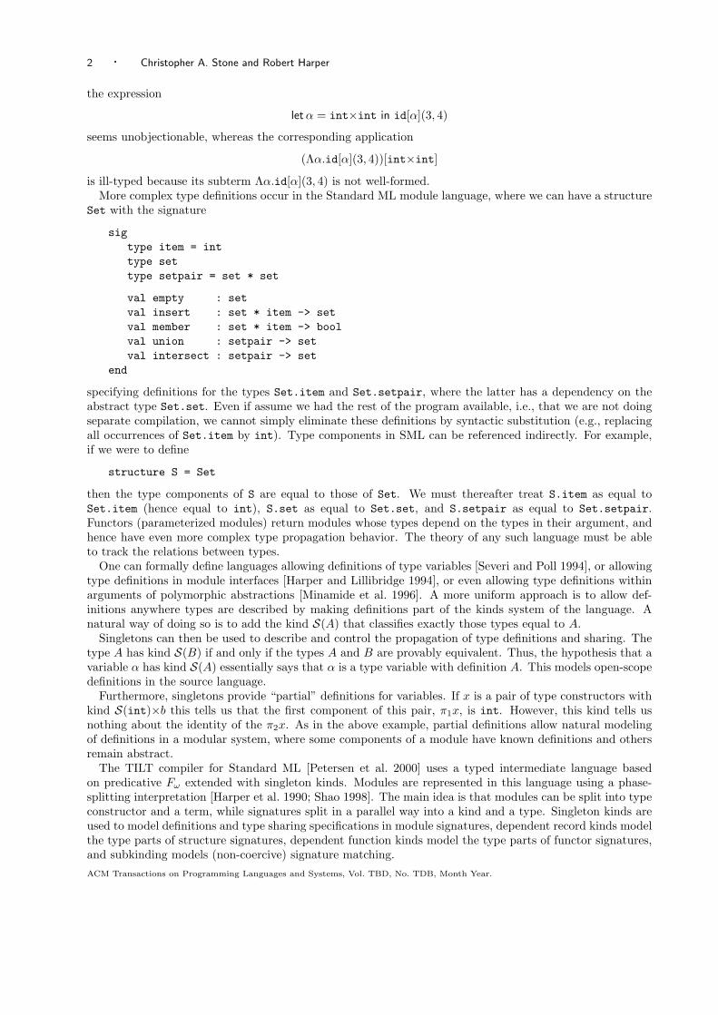
Set with the signature

sigtype item = inttype settype setpair = set * set

val empty : setval insert : set * item -> setval member : set * item -> boolval union : setpair -> setval intersect : setpair -> set

end

specifying definitions for the types Set.item and Set.setpair, where the latter has a dependency on theabstract type Set.set. Even if assume we had the rest of the program available, i.e., that we are not doingseparate compilation, we cannot simply eliminate these definitions by syntactic substitution (e.g., replacingall occurrences of Set.item by int). Type components in SML can be referenced indirectly. For example,if we were to define

structure S = Set

then the type components of S are equal to those of Set. We must thereafter treat S.item as equal toSet.item (hence equal to int), S.set as equal to Set.set, and S.setpair as equal to Set.setpair.Functors (parameterized modules) return modules whose types depend on the types in their argument, andhence have even more complex type propagation behavior. The theory of any such language must be ableto track the relations between types.

One can formally define languages allowing definitions of type variables [Severi and Poll 1994], or allowingtype definitions in module interfaces [Harper and Lillibridge 1994], or even allowing type definitions withinarguments of polymorphic abstractions [Minamide et al. 1996]. A more uniform approach is to allow def-initions anywhere types are described by making definitions part of the kinds system of the language. Anatural way of doing so is to add the kind S(A) that classifies exactly those types equal to A.

Singletons can then be used to describe and control the propagation of type definitions and sharing. Thetype A has kind S(B) if and only if the types A and B are provably equivalent. Thus, the hypothesis that avariable α has kind S(A) essentially says that α is a type variable with definition A. This models open-scopedefinitions in the source language.

Furthermore, singletons provide “partial” definitions for variables. If x is a pair of type constructors withkind S(int)×b this tells us that the first component of this pair, π1x, is int. However, this kind tells usnothing about the identity of the π2x. As in the above example, partial definitions allow natural modelingof definitions in a modular system, where some components of a module have known definitions and othersremain abstract.

The TILT compiler for Standard ML [Petersen et al. 2000] uses a typed intermediate language basedon predicative Fω extended with singleton kinds. Modules are represented in this language using a phase-splitting interpretation [Harper et al. 1990; Shao 1998]. The main idea is that modules can be split into typeconstructor and a term, while signatures split in a parallel way into a kind and a type. Singleton kinds areused to model definitions and type sharing specifications in module signatures, dependent record kinds modelthe type parts of structure signatures, dependent function kinds model the type parts of functor signatures,and subkinding models (non-coercive) signature matching.ACM Transactions on Programming Languages and Systems, Vol. TBD, No. TDB, Month Year.

Extensional Equivalence and Singleton Types · 3

A crucial property of typed intermediate languages is that type checking be decidable. For many languagesthis reduces to checking equivalence of types. We are therefore concerned with establishing the decidabilityof equivalence in the presence of singletons, ideally by showing the correctness of a practical algorithm.

1.1 From Singleton Kinds to Singleton Types

Since ordinary expressions in the TILT typed intermediate language have no effect on equivalence of typeconstructors, we abstract the problem to a simpler two-level calculus λΠΣS

≤ and study term equivalence in alanguage with singleton and dependent types. These levels correspond to the type constructors and kinds ofTILT, but λΠΣS

≤ is of general interest in its own right.In Section 2, we define the λΠΣS

≤ calculus. The fact that any two terms having the same singleton typeare equal is a form of extensionality, and so it seems natural for λΠΣS

≤ to define equivalence of functions andpairs extensionally as well.

This leads to a very interesting equational theory; for example, β-equivalence becomes admissible. Moreimportantly, whether two terms are provably equivalent can depend on both the typing context and —less obviously — on the type at which the terms are compared. The identity function and a functionalways returning some constant c are naturally inequivalent, but if we consider them as functions of typeS(c) → S(c), then extensionally the two functions are equal; they return the same result for all argumentsof type S(c). The common method of implementing equivalence via context-insensitive rewrite rules is thusnot directly applicable for our calculus.

Section 3 contains proofs for many standard properties of the λΠΣS≤ calculus, such as preservation of well-

typedness under substitutions and the admissibility of useful rules. We show that although the definition ofλΠΣS≤ includes only restricted form of singleton type, more general singletons are definable.In Section 4 we present an algorithm for computing normal forms of terms. This is broadly similar to the

algorithm used in work on Typed Operational Semantics [Goguen 1994], but our algorithm is type-directed(normalization is guided by the type at which we are normalizing), and we compute long normal forms.

We then show the correctness of this normalization algorithm. Our argument relies on a novel form ofset-based Kripke logical relations to handle the complications induced by singleton and dependent types.Intuitively, rather than define a logical binary equivalence relation, we work directly with (subsets of) thecorresponding equivalence classes.

Given the correctness of normalization, in Section 5 we present a more efficient and more direct binaryequivalence algorithm.

In Section 6 we sketch correct algorithms for deciding the remaining type and term-level judgments (e.g.,given a well-formed context and a term M , determine whether there is a type A such that M is well-formedwith type A). We show all the algorithms are sound and complete with respect to the language definition,and are terminating. These algorithms form the core of the TILT compiler’s typechecking implementation.

Finally, we survey the related literature and conclude.

2. THE λΠΣS≤ CALCULUS

2.1 Syntax of λΠΣS≤

The abstract syntax of λΠΣS≤ is shown in Figure 1. As usual, we work modulo renaming of bound variables.

The meaning of each construct is explained in tandem with the static semantics (type system) of λΠΣS≤

below.

2.1.1 Substitutions. The notation FV(phrase) refers to the set of free variables in phrase and is definedFigure 2 by induction on syntax.

Also, the static semantics uses the notion of capture-avoiding substitution. We use the metavariable γ tostand for an arbitrary mapping from term variables to terms. The notation γ(phrase) is used to representthe result of applying γ to all free variables in the phrase phrase. The substitution which sends x to M andleaves all other variables unchanged is written [M/x]. If γ is a substitution, then γ[x7→M ] stands for themapping which sends x to M and behaves like γ for all other variables.

2.1.2 Typing Contexts. A typing context Γ (or simply context when this is unambiguous) representsassumptions for the types of free term variables. It is represented as a finite sequence of variable/classifier

ACM Transactions on Programming Languages and Systems, Vol. TBD, No. TDB, Month Year.


Typing Contexts Γ,∆ ::= • Empty context| Γ, x : A

Types A, σ ::= b Base type| S(M) Singleton type| Πx:A′. A′′ Dependent function type| Σx:A′. A′′ Dependent pair type

Terms M,N ::= ci Constants| x, y, . . . Variables

| λx:A′.M Function

| MM ′ Application| 〈M ′,M ′′〉 Pair

| πiM Projection

Fig. 1. Syntax of the λΠΣS≤ Calculus

FV(b) := ∅FV(S(M)) := FV(M)FV(Πx:A′. A′′) := FV(A′) ∪ (FV(A′′) \ {x})FV(Σx:A′. A′′) := FV(A′) ∪ (FV(A′′) \ {x})

FV(c) := ∅FV(x) := {x}FV(λx:A.M) := FV(A) ∪ (FV(M) \ {x})FV(MM ′) := FV(M) ∪ FV(M ′)FV(〈M ′,M ′′〉) := FV(M ′) ∪ FV(M ′′)FV(πiM) := FV(M)

Fig. 2. Free-Variable Sets for Types and Terms

associations. Typing contexts in λΠΣS≤ are intrinsically ordered sequences because of the dependencies

introduced by singletons: types can refer to term variables appearing earlier in the context.

2.2 Static Semantics of λΠΣS≤

The context validity judgment Γ ` ok determines when a typing context Γ is well-formed: every typeappearing in the context must be well-formed with respect to the preceding segment of the context.

The side-condition in Rule 2 ensures that variables are not bound in a context more than once; the notationdom(Γ) is used to represent the set of all term variables assigned types by Γ. It follows that well-formedtyping contexts can also be viewed as finite functions: Γ(x) represents the type associated with x in Γ.Because contexts are finite sequences, there is an obvious definition for appending any two contexts; theresult of appending Γ1 and Γ2 is written Γ1,Γ2.

We define a (purely syntactic) partial order on contexts. The subset relation Γ1 ⊆ Γ2 on contexts holds ifΓ1(x) = Γ2(x) for every x ∈ dom(Γ1). Thus if Γ1 ⊆ Γ2 then dom(Γ1) ⊆ dom(Γ2) and Γ1 appears as a (notnecessarily consecutive) subsequence of Γ2. We also write Γ2 ⊇ Γ1 to mean Γ1 ⊆ Γ2.

2.2.1 Types. The type validity judgment Γ ` A specifies when a type A is well-formed with respect to agiven typing context Γ.

The premise Γ ` ok in Rule 3 for the base type b ensures that in any proof of a judgment Γ ` A there isstrict subderivation proving Γ ` ok. A similar property will hold for all of the judgments (Proposition 3.1).

Well-formed singleton types in λΠΣS≤ are restricted to contain only terms of the base type b, as shown in

Rule 4. However, more general singleton types SA(M), classifying terms equivalent to M and type A, aredefinable in this calculus (see Section 2.3).

Rules 5 and 6 for Π and Σ types (dependent types of functions of terms and pairs of terms respectively)are standard. Πx:A′. A′′ is the type of all functions which map an argument x of type A′ to a result of typeA′′, where A′′ may depend on x. Similarly, Σx:A′. A′′ is the type of all pairs of terms whose first componentACM Transactions on Programming Languages and Systems, Vol. TBD, No. TDB, Month Year.


Well-Formed Context

• ` ok(1)

Γ ` AΓ, x : A ` ok

(x 6∈ dom(Γ)) (2)

Well-Formed Type

Γ ` ok

Γ ` b(3)

Γ ` M : b

Γ ` S(M)(4)

Γ, x : A′ ` A′′

Γ ` Πx:A′. A′′(5)

Γ, x : A′ ` A′′

Γ ` Σx:A′. A′′(6)

Subtyping

Γ ` M : b

Γ ` S(M) ≤ b(7)

Γ ` M1 ≡ M2 : b

Γ ` S(M1) ≤ S(M2)(8)

Γ ` ok

Γ ` b ≤ b(9)

Γ ` Πx:A′1. A′′1

Γ ` A′2 ≤ A′1 Γ, x : A′2 ` A′′1 ≤ A′′2Γ ` Πx:A′1. A

′′1 ≤ Πx:A′2. A

′′2

(10)

Γ ` Σx:A′2. A′′2

Γ ` A′1 ≤ A′2 Γ, x : A′1 ` A′′1 ≤ A′′2Γ ` Σx:A′1. A

′′1 ≤ Σx:A′2. A

′′2

(11)

Type Equivalence

Γ ` ok

Γ ` b ≡ b(12)

Γ ` M1 ≡ M2 : b

Γ ` S(M1) ≡ S(M2)(13)

Γ ` A′1 ≡ A′2 Γ, x : A′1 ` A′′1 ≡ A′′2Γ ` Πx:A′1. A

′′1 ≡ Πx:A′2. A

′′2

(14)

Γ ` A′1 ≡ A′2 Γ, x : A′1 ` A′′1 ≡ A′′2Γ ` Σx:A′1. A

′′1 ≡ Σx:A′2. A

′′2

(15)

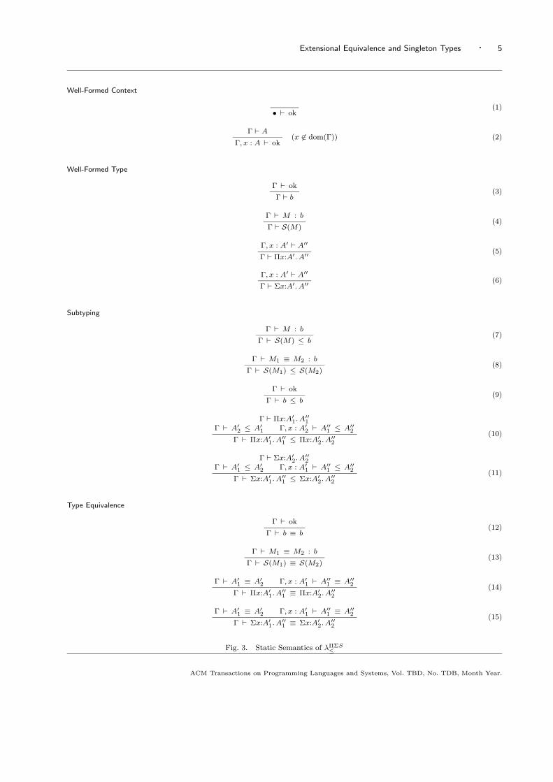
Fig. 3. Static Semantics of λΠΣS≤



Well-Formed Term

Γ ` ok

Γ ` ci : b(16)

Γ ` ok

Γ ` x : Γ(x)(x ∈ dom(Γ)) (17)

Γ, x : A′ ` M : A′′

Γ ` λx:A′.M : Πx:A′. A′′(18)

Γ ` M : Πx:A′. A′′ Γ ` M ′ : A′

Γ ` MM ′ : [M ′/x]A′′(19)

Γ ` Σx:A′. A′′

Γ ` M ′ : A′ Γ ` M ′′ : [M ′/x]A′′

Γ ` 〈M ′,M ′′〉 : Σx:A′. A′′(20)

Γ ` M : Σx:A′. A′′

Γ ` π1M : A′(21)

Γ ` M : Σx:A′. A′′

Γ ` π2M : [π1M/x]A′′(22)

Γ ` M : b

Γ ` M : S(M)(23)

Γ ` Σx:A′. A′′

Γ ` π1M : A′ Γ ` π2M : [π1M/x]A′′

Γ ` M : Σx:A′. A′′(24)

Γ, x : A′ ` M x : A′′

Γ ` M : Πx:A′. B′′ Γ ` Πx:A′. B′′

Γ ` M : Πx:A′. A′′(25)

Γ ` M : A1 Γ ` A1 ≤ A2

Γ ` M : A2(26)

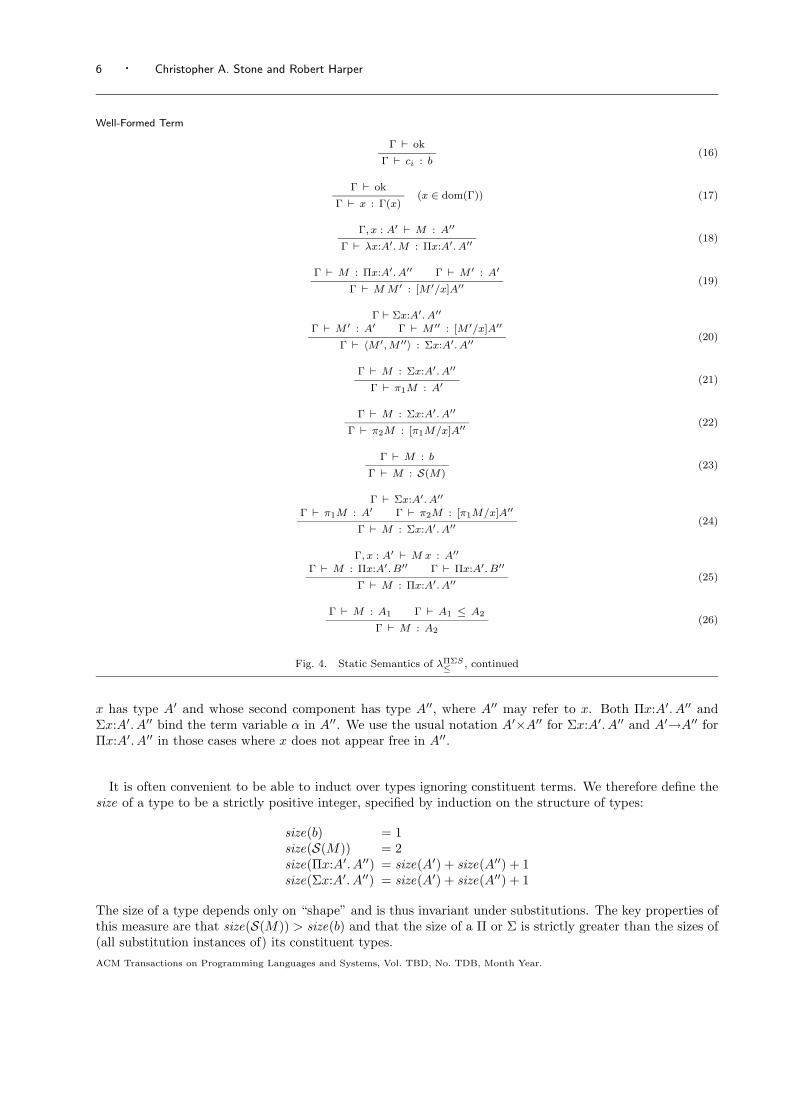
Fig. 4. Static Semantics of λΠΣS≤ , continued

x has type A′ and whose second component has type A′′, where A′′ may refer to x. Both Πx:A′. A′′ andΣx:A′. A′′ bind the term variable α in A′′. We use the usual notation A′×A′′ for Σx:A′. A′′ and A′→A′′ forΠx:A′. A′′ in those cases where x does not appear free in A′′.

It is often convenient to be able to induct over types ignoring constituent terms. We therefore define thesize of a type to be a strictly positive integer, specified by induction on the structure of types:

size(b) = 1size(S(M)) = 2size(Πx:A′. A′′) = size(A′) + size(A′′) + 1size(Σx:A′. A′′) = size(A′) + size(A′′) + 1

The size of a type depends only on “shape” and is thus invariant under substitutions. The key properties ofthis measure are that size(S(M)) > size(b) and that the size of a Π or Σ is strictly greater than the sizes of(all substitution instances of) its constituent types.ACM Transactions on Programming Languages and Systems, Vol. TBD, No. TDB, Month Year.


Term Equivalence

Γ ` M : A

Γ ` M ≡ M : A(27)

Γ ` M2 ≡ M1 : A

Γ ` M1 ≡ M2 : A(28)

Γ ` M1 ≡ M2 : A Γ ` M2 ≡ M3 : A

Γ ` M1 ≡ M3 : A(29)

Γ ` A′1 ≡ A′2 Γ, x : A′1 ` M1 ≡ M2 : A′′

Γ ` λx:A′1.M1 ≡ λx:A′2.M2 : Πx:A′1. A′′ (30)

Γ ` M1 ≡ M2 : Πx:A′. A′′ Γ ` M ′1 ≡ M ′2 : A′

Γ ` M1 M ′1 ≡ M2 M ′2 : [M ′1/x]A′′(31)

Γ ` M1 ≡ M2 : Σx:A′. A′′

Γ ` π1M1 ≡ π1M2 : A′(32)

Γ ` M1 ≡ M2 : Σx:A′. A′′

Γ ` π2M1 ≡ π2M2 : [π1M1/x]A′′(33)

Γ ` Σx:A′. A′′

Γ ` M ′1 ≡ M ′2 : A′

Γ ` M ′′1 ≡ M ′′2 : [M ′1/x]A′′

Γ ` 〈M ′1,M ′′1 〉 ≡ 〈M ′2,M ′′2 〉 : Σx:A′. A′′(34)

Γ ` Σx:A′. A′′

Γ ` π1M1 ≡ π1M2 : A′

Γ ` π2M1 ≡ π2M2 : [π1M1/x]A′′

Γ ` M1 ≡ M2 : Σx:A′. A′′(35)

Γ, x : A′ ` M1 x ≡ M2 x : A′′

Γ ` M1 : Πx:A′. B′′1 Γ ` M2 : Πx:A′. B′′2Γ ` M1 ≡ M2 : Πx:A′. A′′

(36)

Γ ` M1 ≡ M2 : A1 Γ ` A1 ≤ A2

Γ ` M1 ≡ M2 : A2(37)

Γ ` M : S(N)

Γ ` M ≡ N : S(N)(38)

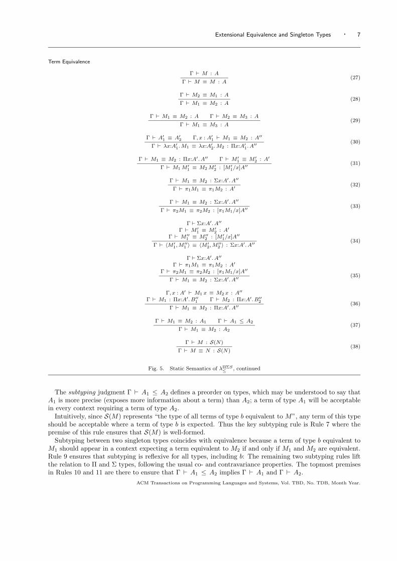
Fig. 5. Static Semantics of λΠΣS≤ , continued

The subtyping judgment Γ ` A1 ≤ A2 defines a preorder on types, which may be understood to say thatA1 is more precise (exposes more information about a term) than A2; a term of type A1 will be acceptablein every context requiring a term of type A2.

Intuitively, since S(M) represents “the type of all terms of type b equivalent to M”, any term of this typeshould be acceptable where a term of type b is expected. Thus the key subtyping rule is Rule 7 where thepremise of this rule ensures that S(M) is well-formed.

Subtyping between two singleton types coincides with equivalence because a term of type b equivalent toM1 should appear in a context expecting a term equivalent to M2 if and only if M1 and M2 are equivalent.Rule 9 ensures that subtyping is reflexive for all types, including b: The remaining two subtyping rules liftthe relation to Π and Σ types, following the usual co- and contravariance properties. The topmost premisesin Rules 10 and 11 are there to ensure that Γ ` A1 ≤ A2 implies Γ ` A1 and Γ ` A2.



Type equivalence, denoted Γ ` A1 ≡ A2, is essentially a symmetrized version of subtyping. We showlater that Γ ` A1 ≡ A2 if and only if Γ ` A1 ≤ A2 and Γ ` A2 ≤ A1, and a reasonable alternative wouldbe to make this the definition of type equivalence.

2.2.2 Terms. The term validity judgment Γ ` M : A determines when a term M is well-formed incontext Γ and satisfies the classifying type A. Rules 16–22 are the usual rules for a a dependently-typedλ-calculus with pairing, projections, and a base type.

Rule 23 is the obvious introduction form for singletons. Rules 24 and 25 are somewhat less familiar, butanalogous rules often appear in literature studying Standard ML modules, e.g., the non-standard structure-typing rule of Harper, Mitchell, and Moggi [Harper et al. 1990], the VALUE rules of Harper and Lillib-ridge’s translucent sums [Harper and Lillibridge 1994], the strengthening operation of Leroy’s manifest typesystem [Leroy 1994], the “self” rule of Leroy’s applicative functors [Leroy 1995], and the REFL rule of As-pinall [Aspinall 2000]. The two rules can be justified as reflexive instances of extensionality (Rules 35 and 36below) and ensure that a term has every type that its η-expansion does:

In most dependently-typed calculi such rules would be admissible rather than part of the system’s defini-tion. However, in λΠΣS

≤ they allow terms to be given strictly more precise types. For example, assume thatx : b×b. In the absence of Rule 24, the most precise (and only) type of x is b×b. Using Rule 24 though, wecan show

x : b×b ` x : S(π1x)×S(π2x).

That is, x has “the type of pairs whose first component is equal to the first component of x and whose secondcomponent is equal to the second component of x”. This type is much more precise and informative b×b,and it is entirely reasonable that x itself ought to satisfy that type. (By extensionality the only pair withthis type is x itself, and in fact Rules 24 and 25 will be critical for encoding singleton types for arbitraryterms.) The rules therefore can be viewed as extending singleton introduction to higher types.

We conjecture that the lower two premises in Rule 25 could be replaced by the much simpler side-conditionx 6∈ FV(M), but we then become unable to prove the existence of most-specific types (see Section 3.4). Theformulation here makes explicit that Rule 25 yields more-precise Π types for terms only by making thecodomain more precise, rather than by weakening the domain type.

The final term well-formedness rule is the subsumption rule, Rule 26.

Term equivalence defines a notion of equality (interchangeability) for terms. The judgment Γ ` M1 ≡M2 : A expresses the fact that M1 and M2 are equivalent terms of type A under context Γ. Equivalenceis highly context-sensitive: whether Γ ` M1 ≡ M2 : A is provable depends not only on M1 and M2, butalso on the types of free variables (given by Γ) and the type A at which the two terms are being compared.We therefore cannot define equivalence indirectly via context-insensitive rewrite rules, but must axiomatizeit directly.

Equivalence is first defined to be a reflexive, symmetric, and transitive relation (Rules 27–29) and acongruence, i.e., replacing subparts of a term with equivalent parts yields an equivalent term (Rules 30–34).

There are two extensionality rules, Rule 35 and 36. If two functions or two pairs cannot be distinguishedby their uses then they are considered equivalent. In particular, two pairs are equivalent if they haveequivalent first and second components and two functions are equivalent if they return equivalent results forall arguments. If Rule 25 were simplified as discussed above then the last two premises could be replacedwith the side condition x 6∈ (FV(M1) ∪ FV(M2)).

We also have subsumption for equivalence (Rule 37) just as for well-formedness.

Interestingly, an easy inductive argument shows that the rules given so far merely define term equivalenceto be syntactic identity up to renaming of bound variables. However, adding Rule 38, the elimination rulefor singleton types, makes equivalence non-trivial and justifies the presence of each of the above rules:

This completes the definition of term equivalence. It may be initially surprising that there are no equiva-lence rules for reducing function applications or projections from pairs (i.e., β-like rules). It turns out thatthese are admissible in the presence of singleton types and Rule 38. The full details are in Section 2.3 andSection 3.3, but we sketch one example here. It is clear that

` 〈c, c2〉 : S(c)×S(c2).ACM Transactions on Programming Languages and Systems, Vol. TBD, No. TDB, Month Year.


Then by Rule 21 it follows

` π1〈c, c2〉 : S(c)

and by Rule 38 and subsumption we thus have

` π1〈c, c2〉 ≡ c : b

This same argument can be generalized to projections from arbitrary pairs, and in an analogous fashion toapplications of λ-abstractions.

Given the β-rules, then, the extensionality rules 35 and 36 imply that the usual η-rules are admissible aswell. It is well-known that η-reduction is not confluent in the presence of terminal (unit) types. As unit isa special case of a singleton type, the same behavior appears here as well. For example:

x : b→S(c) ` x ≡ λy:b. c : b→b

holds, as does

x : S(c)→b ` x ≡ λy:S(c). (x c) : S(c)→bAll the terms in these judgments are normal with respect to βη-reduction; compare the right-hand term inthe last judgment with λy:S(c). (x y), the η-expansion of x.

A more obvious consequence of having singletons — and their original motivation — is that they can beused to express definitions for variables. For example, in the following two judgments the context effectivelydefines x to be c.

x : S(c) ` x ≡ c : bx : S(c) ` 〈x, c〉 ≡ 〈c, x〉 : b×b

But the system is not restricted merely to giving simple definitions to variables. In the provable judgment

x : b×S(c) ` π2x ≡ c : b

the context partially defines x; it is known to be a pair and its second component is (equivalent to) c, butthis does not give a definition for x as a whole. Alternatively, this could be thought of as giving π2x thedefinition c without giving a definition for π1x.

Similarly, in the provable judgments

x : (Σy:b.S(y)) ` π1x ≡ π2x : bx : (Σy:b.S(y)) ` x ≡ 〈π1x, π1x〉 : b×b.

the assumption governing x requires that it be a pair whose first component y has type b and whose secondcomponent is equal to the first; that is, a pair with two equal components of type b. This gives a definitionto π2x, namely π1x, without further specifying the contents of these two equal components.

Now because of subtyping and subsumption, terms do not have unique types. The equational systempresented here has the relatively unusual property that equivalence of two terms depends on the type atwhich they are compared. Two terms may be equivalent at one type but not at another; for example, onecannot prove

` λx:b. x ≡ λx:b. c : b→band this is fortunate, as this would lead to an inconsistent equational theory where, for example, c and c2were provably equivalent. However, by subsumption these two functions both have type S(c)→b and thejudgment

` λx:b. x ≡ λx:b. c : S(c)→bis provable; the proof uses extensionality and the fact that the two functions provably agree on all argumentsof type S(c), i.e., when applied to only the argument c.

The classifying type at which terms are compared may depend on the context of their occurrence. Forexample, it follows immediately from the previous equation that

y : (S(c)→b)→b ` y (λx:b. x) ≡ y (λx:b. c) : bACM Transactions on Programming Languages and Systems, Vol. TBD, No. TDB, Month Year.


is also provable. The type of y guarantees that it will apply its argument only to the term c, so it cannotmatter whether y is given λx:b. x or λx:b. c. In contrast, the judgment

y : (b→b)→b ` y (λx:b. x) ≡ y (λx:b. c) : b

is not provable because the context makes a weaker assumption about y.

2.3 Admissible Rules and Labeled Singletons

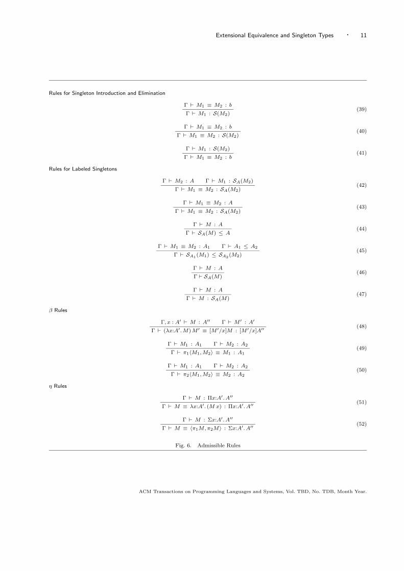
We next turn to number of interesting and useful rules which are admissible in our system, shown inFigure 6. Rules 39–41 are variant introduction and elimination rules for singleton types

Next, in λΠΣS≤ the type S(M) is well-formed if and only if M is of the base type b. This initially seems

restrictive, as one might expect to find singleton types of the form SA(M) representing the type of all termsequivalent to M when compared at type A. These would be necessary, for example, to model definitions ofterm-level functions. However, these labeled singletons are already definable within λΠΣS

≤ .One possible definition, defined by induction on the size of the type label, is as follows:.1

Sb(M) := S(M)SS(M ′)(M) := S(M)SΠx:A1. A2(M) := Πx:A1. (SA2(M x))SΣx:A1. A2(M) := SA1(π1M)× S[π1M/x]A2(π2M)

For example, if y has type b→b, then Sb→b(y) is defined to be Πx:b.S(y x). This can be interpreted as “thetype of all functions that, when applied, yield the same answer as y does”, or “the type of all functions thatagree pointwise with y”. By extensionality, any such function is provably equivalent to y. The non-standardtyping rules mentioned in Section 2 are vital in proving that y has this type.

Rules 42–47 are admissible, showing that the labeled singleton types do behave appropriately; proofs aredeferred to Section 3.3.

Because these labeled singletons are defined rather than primitive, one must be careful to note thatΓ ` SA(M) does not imply Γ ` M : A. For example, if c1 and c2 are distinct constants then accordingto our definition we have SS(c2)(c1) = S(c1), and therefore ` SS(c2)(c1) even though c1 cannot be shown tohave type S(c2). This explains the premise Γ ` M2 : A in Rule 42.

Next, a remarkable observation of Aspinall [Aspinall 1995] is that the β-rule for function applications isadmissible in the presence of singletons. In λΠΣS

≤ , which contains pairs, the projection rules are admissibleas well. The resulting equivalences appear as admissible rules 48–50.

Finally, in the presence of both β-equivalence and extensionality, η-rules for functions and pairs (Rules 51and 52) are admissible.

3. DECLARATIVE PROPERTIES

In this section we present several basic properties of the λΠΣS≤ calculus. From these we derive the definability

of generalized singleton types, and the admissibility of the rules given in Section 2.3.

3.1 Preliminaries

We start with a number of very simple properties, each of which follows easily by induction on derivations.If we define typing-context-free judgment forms J :

J ::= ok | Γ1 ≡ Γ2 | A | A1 ≤ A2 | A1 ≡ A2 | M : A | M1 ≡M2 : A

then given a context Γ one can construct a λΠΣS≤ judgment Γ ` J . The substitution γJ is defined by applying

the substitution to the individual types and terms appearing in J , while the free variable computation FV(J )is similarly defined as the union of the free variables of the phrases in J .

Proposition 3.1 (Subderivations)(1 ) Every proof of Γ ` J contains a subderivation Γ ` ok.(2 ) Every proof of Γ1, x : A,Γ2 ` J contains a strict subderivation Γ1 ` A.

1Since types only matter up to equivalence, these definitions are not unique. One could equally well define SS(M′)(M) to beS(M ′), or define SΣx:A1. A2 (M) to be Σx:SA1 (π1M).SA2 (π2M).



Rules for Singleton Introduction and Elimination

Γ ` M1 ≡ M2 : b

Γ ` M1 : S(M2)(39)

Γ ` M1 ≡ M2 : b

Γ ` M1 ≡ M2 : S(M2)(40)

Γ ` M1 : S(M2)

Γ ` M1 ≡ M2 : b(41)

Rules for Labeled Singletons

Γ ` M2 : A Γ ` M1 : SA(M2)

Γ ` M1 ≡ M2 : SA(M2)(42)

Γ ` M1 ≡ M2 : A

Γ ` M1 ≡ M2 : SA(M2)(43)

Γ ` M : A

Γ ` SA(M) ≤ A(44)

Γ ` M1 ≡ M2 : A1 Γ ` A1 ≤ A2

Γ ` SA1 (M1) ≤ SA2 (M2)(45)

Γ ` M : A

Γ ` SA(M)(46)

Γ ` M : A

Γ ` M : SA(M)(47)

β Rules

Γ, x : A′ ` M : A′′ Γ ` M ′ : A′

Γ ` (λx:A′.M)M ′ ≡ [M ′/x]M : [M ′/x]A′′(48)

Γ ` M1 : A1 Γ ` M2 : A2

Γ ` π1〈M1,M2〉 ≡ M1 : A1(49)

Γ ` M1 : A1 Γ ` M2 : A2

Γ ` π2〈M1,M2〉 ≡ M2 : A2(50)

η Rules

Γ ` M : Πx:A′. A′′

Γ ` M ≡ λx:A′. (M x) : Πx:A′. A′′(51)

Γ ` M : Σx:A′. A′′

Γ ` M ≡ 〈π1M,π2M〉 : Σx:A′. A′′(52)

Fig. 6. Admissible Rules



(3 ) If Γ ` MM ′ : B then there is a strict subderivation of the form Γ ` M : A for some type A.(4 ) If Γ ` πiM : B then there is a strict subderivation of the form Γ ` M : A for some type A.

Proposition 3.2If Γ ` J then FV(J ) ⊆ dom(Γ).

Proposition 3.3 (Reflexivity)(1 ) If Γ ` A then Γ ` A ≡ A.(2 ) If Γ ` A then Γ ` A ≤ A.

Proposition 3.4 (Weakening of Typing Contexts)(1 ) If Γ1 ` J and Γ1 ⊆ Γ2 and Γ2 ` ok, then Γ2 ` J .(2 ) If Γ1, x : A2,Γ2 ` J and Γ1 ` A1 ≤ A2 and Γ1 ` A1 then Γ1, x : A1,Γ2 ` J .

Later we show that the assumption Γ1 ` A1 in the statement of Weakening is redundant, being alreadyimplied by Γ1 ` A1 ≤ A2.

Definition 3.5The judgment θ ` γ : Γ holds if and only if the following conditions all hold:

(1 ) θ ` ok(2 ) ∀x ∈ dom(Γ). θ ` γx : γ(Γ(x))

Proposition 3.6 (Substitution)(1 ) If Γ ` J and θ ` γ : Γ then θ ` γ(J ).(2 ) If Γ1, x : A,Γ2 ` ok and Γ1 ` M : A then Γ1, [M/x]Γ2 ` ok.

3.2 Validity and Functionality

We next show two highly useful properties of the calculus. Validity is the property that any phrase appearingwithin a provable judgment is well-formed (e.g., if Γ ` M1 ≡ M2 : A then Γ ` ok and Γ ` A andΓ ` M1 : A and Γ ` M2 : A). Functionality states that applying equivalent substitutions to phrasesrelated by equivalence or subtyping yields similarly related phrases.

The rules have been structured to assume validity for premises and guarantee and preserve validity forconclusions. A simple proof, however, is hindered by the presence of dependencies in types. The directapproach by induction on derivations fails because of cases such as Rule 33:

Γ ` M1 ≡ M2 : Σx:A′. A′′

Γ ` π2M1 ≡ π2M2 : [π1M1/x]A′′.

Here we need to show Γ ` π2M2 : [π1M1/x]A′′ but from the inductive hypothesis and Rule 22 we have onlyΓ ` π2M2 : [π1M2/x]A′′. The desired result would follow, however, if we knew that Γ ` [π1M2/x]A′′ ≤ [π1M1/x]A′′.Since Γ ` π1M2 ≡ π1M1 : A′, the subtyping judgment required follows from functionality.

This suggests one should first prove functionality. The most general form of functionality cannot bedirectly proved in the absence of validity, but the proof does go through for the restricted case of equivalentsubstitutions being applied to a single phrase. This suffices to show validity, and together these allow asimple proof of general functionality.

Definition 3.7The judgment θ ` γ1 ≡ γ2 : Γ holds if and only if the following conditions all hold:

(1 ) θ ` γ1 : Γ and θ ` γ2 : Γ(2 ) ∀x ∈ dom(Γ). θ ` γ1x ≡ γ2x : γ1(Γ(x))

Proposition 3.8 (Simple Functionality)(1 ) If Γ ` A and θ ` γ1 ≡ γ2 : Γ then θ ` γ1A ≡ γ2A.(2 ) If Γ ` A and θ ` γ1 ≡ γ2 : Γ then θ ` γ1A ≤ γ2A.(3 ) If Γ ` M : A and θ ` γ1 ≡ γ2 : Γ then θ ` γ1M ≡ γ2M : γ1A.

Proof. By induction on the proof of the first premise.



Proposition 3.9 (Validity)(1 ) If Γ ` A1 ≤ A2 then Γ ` A1 and Γ ` A2.(2 ) If Γ ` A1 ≡ A2 then Γ ` A1 and Γ ` A2.(3 ) If Γ ` M : A then Γ ` A.(4 ) If Γ ` M1 ≡ M2 : A then Γ ` M1 : A, Γ ` M2 : A, and Γ ` A.

Proof. By induction on derivations. There are only a few interesting cases, those for Rules 31 and 33.We show just the latter here:

Γ ` M1 ≡ M2 : Σx:A′. A′′

Γ ` π2M1 ≡ π2M2 : [π1M1/x]A′′

By the inductive hypothesis, Γ ` M1 : Σx:A′. A′′ and Γ ` M2 : Σx:A′. A′′

and Γ ` Σx:A′. A′′. By inversion of Rule 5, Γ, x : A′ ` A′′. Then Γ ` π2M1 : [π1M1/x]A′′ by Rule 22, soby Proposition 3.6 we have Γ ` [π1M1/x]A′′. Since Γ ` π1M2 : A′ and Γ ` π1M1 : A′ andΓ ` π1M2 ≡ π1M1 : A′, we have Γ ` [π1M2/x] ≡ [π1M1/x] : (Γ, x : A′). By Proposition 3.8 we haveΓ ` [π1M2/x]A′′ ≤ [π1M1/x]A′′. Thus by subsumption and the fact that Γ ` π2M2 : [π1M2/x]A′′ byRule 22, we have Γ ` π2M2 : [π1M1/x]A′′.

Once we have validity, the following propositions each follow by an easy induction on derivations.

Proposition 3.10 (Antisymmetry of Subtyping)Γ ` A1 ≤ A2 and Γ ` A2 ≤ A1 if and only if Γ ` A1 ≡ A2.

Proposition 3.11 (Symmetry and Transitivity of Type Equivalence)(1 ) If Γ ` A1 ≡ A2 then Γ ` A2 ≡ A1

(2 ) If Γ ` A1 ≡ A2 and Γ ` A2 ≡ A3 then Γ ` A1 ≡ A3.

Proposition 3.12 (Transitivity of Subtyping)If Γ ` A1 ≤ A2 and Γ ` A2 ≤ A3 then Γ ` A1 ≤ A3.

Proof. By induction on size(A1) + size(A2) + size(A3)

Proposition 3.13 (Full Functionality)(1 ) If Γ ` M1 ≡ M2 : A and θ ` γ1 ≡ γ2 : Γ then θ ` γ1M1 ≡ γ2M2 : γ1A.(2 ) If Γ ` A1 ≡ A2 and θ ` γ1 ≡ γ2 : Γ then θ ` γ1A1 ≡ γ2A2.(3 ) If Γ ` A1 ≤ A2 and θ ` γ1 ≡ γ2 : Γ then θ ` γ1A1 ≤ γ2A2.

Proof. We show the proof for just the first part; the last two parts follow similarly.Assume Γ ` M1 ≡ M2 : A and θ ` γ1 ≡ γ2 : Γ. By substitution, θ ` γ1M1 ≡ γ1M2 : γ1A. ByProposition 3.9 we have Γ ` M2 : A, and so by Proposition 3.8, θ ` γ1M2 ≡ γ2M2 : γ1A. ByProposition 3.11, θ ` γ1M1 ≡ γ2M2 : γ1A.

3.3 Proofs of Admissibility

We now have enough technical machinery to prove the admissibility of Rules 39–52.

Lemma 3.14γ(SA(M)) = SγA(γM).

Proposition 3.15The rules from Section 2.3 are all admissible

Proof.

—Case: Rules 39–41. By Proposition 3.9 and subsumption.—Case: Rule 42.

Γ ` M2 : A Γ ` M1 : SA(M2)Γ ` M1 ≡ M2 : SA(M2)

By induction on the size of A.ACM Transactions on Programming Languages and Systems, Vol. TBD, No. TDB, Month Year.


—Case A = b and SA(M2) = S(M2). By Rule 38, Γ ` M1 ≡ M2 : S(M2).—Case A = S(N) and SA(M2) = S(M2). By Rule 38, Γ ` M1 ≡ M2 : S(M2).—Case A = Πx:A′. A′′ and SA(M2) = Πx:A′.SA′′(M2 x). By Rule 19 we have

Γ, x : A′ ` M1 x : SA′′(M2 x) and Γ, x : A′ ` M2 x : A′′. By the inductive hypothesis,Γ, x : A′ ` M1 x ≡ M2 x : SA′′(M2 x). Therefore by Rule 36 we haveΓ ` M1 ≡ M2 : Πx:A′.SA′′(M2 x).

—A = Σx:A′. A2 and SA(M2) = (SA′(π1M2))×(S[π1M2/x]A′′(π2M2)). Then Γ ` π1M1 : SA′(π1M2) andΓ ` π2M1 : S[π1M1/x]A′′(π2M2). Γ ` π1M2 : A′ and Γ ` π2M2 : [π1M2/x]A′, so by the inductivehypothesis, Γ ` π1M1 ≡ π1M2 : SA′(π1M2) and Γ ` π2M1 ≡ π2M2 : S[π1M1/x]A′′(π2M2). ByRule 35 we have Γ ` M1 ≡ M2 : (SA′(π1M2))×(S[π1M2/x]A′′(π2M2)).

—Case: Rule 43.

Γ ` M1 ≡ M2 : AΓ ` M1 ≡ M2 : SA(M2)

By induction on the size of A—Case A = b and SA(M2) = S(M2). Γ ` M1 : S(M2) by Rule 39. Then Γ ` M1 ≡ M2 : S(M2) by

Rule 38—Case A = S(N) and SA(M2) = S(M2). Γ ` N : b by Proposition 3.9 and inversion of Rule 4, so

Γ ` S(N) ≤ b. Then Γ ` M1 ≡ M2 : b by subsumption, so Γ ` M1 : S(M2) by Rule 39. ThusΓ ` M1 ≡ M2 : S(M2) by Rule 38.

—Case A = Πx:A′. A′′ and SA(M2) = Πx:A′.SA′′(M2 x). By Rule 31, Γ, x : A′ ` M1 x ≡ M2 x : A′′.By the inductive hypothesis, Γ, x : A′ ` M1 x ≡ M2 x : SA′′(M2 x). By Proposition 3.9 we haveΓ ` M1 : Πx:A′. A′′ and Γ ` M2 : Πx:A′. A′′. Therefore by Rule 36,Γ ` M1 ≡ M2 : Πx:A′.SA′′(M2 x).

—A = Σx:A′. A′′ and SA(M2) = (SA′(π1M2))×(S[π1M2/x]A′′(π2M2)). Then Γ ` π1M1 ≡ π1M2 : A′ andΓ ` π2M1 ≡ π2M2 : [π1M1/x]A′′. By Functionality and subsumption,Γ ` π2M1 ≡ π2M2 : [π1M2/x]A′′. By the inductive hypothesis, Γ ` π1M1 ≡ π1M2 : SA′(π1M2)and Γ ` π2M1 ≡ π2M2 : S[π1M2/x]A′′(π2M2). (Note that size([π1M2/x]A′′) = size(A′′) < size(A).)Therefore by Rule 35 we have Γ ` M1 ≡ M2 : (SA′(π1M2))×(S[π1M2/x]A′′(π2M2)).

—Case: Rule 44.

Γ ` M : AΓ ` SA(M) ≤ A

By induction on the size of A.—Case A = b and SA(M) = S(M). By Rule 7 we have Γ ` Sb(M) ≤ b.—Case A = S(N) and SA(M) = S(M). Then Γ ` M ≡ N : b so Γ ` S(M) ≤ S(N).—Case A = Πx:A1. A2 and SA(M) = Πx:A1.SA2(M x). Then Γ ` A1 and Γ, x : A1 ` M x : A2. By the

inductive hypothesis, Γ, x : A1 ` SA2(M x) ≤ A2. Therefore, Γ ` Πx:A1.SA2(M x) ≤ Πx:A1. A2.—Case A = Σx:A′. A′′ and SA(M) = (SA′(π1M))×(S[π1M/x]A′′(π2M)). By Proposition 3.9 and inversion

of Rule 6 we have Γ, x:A′ ` A′′. Then Γ ` π1M : A′ so by the inductive hypothesis,Γ ` SA′(π1M) ≤ A′. Furthermore, Γ ` π2M : [π1M/x]A′′. By the inductive hypothesis,Γ ` S[π1M/x]A′′(π2M) ≤ [π1M/x]A′′. Also, by Proposition 3.1 and Proposition 3.4,Γ, x : SA′(π1M) ` A′′ ≤ A′′. By Rule 42 we have Γ, x : SA′(π1M) ` x ≡ π1M : SA′(π1M) so byFunctionality we have Γ, x : SA′(π1M) ` [π1M/x]A′′ ≤ A′′. Therefore,Γ ` (SA′(π1M))×(S[π1M/x]A′′(π2M)) ≤ Σx:A′. A′′.

—Case: Rule 45.

Γ ` M1 ≡ M2 : A1 Γ ` A1 ≤ A2

Γ ` SA1(M1) ≤ SA2(M2)

By induction on size(A1).—Case A1 = b or S(M1) and A2 = b or S(M2). Then SA1(M1) = S(M1), SA2(M2) = S(M2), and the

desired conclusion follows by Rule 8.ACM Transactions on Programming Languages and Systems, Vol. TBD, No. TDB, Month Year.


—Case A1 = Πx:A′1. A′′1 and A2 = Πx:A′2. A

′′2 . SAi(Mi) = Πx:A′i.SA′′i (Mi x). By inversion Γ ` A′2 ≤ A′1

and Γ, x : A′2 ` A′′1 ≤ A′′2 . Now Γ, x : A′2 ` M1 x ≡ M2 x : A′′1 . By the inductive hypothesis,Γ, x : A′2 ` SA′′1 (M1 x) ≤ SA′′2 (M2 x). The conclusion follows by Rule 10.

—Case A1 = Σx:A′1. A′′1 and A2 = Σx:A′2. A

′′2 . SA1(M1) = Σx:SA′1(π1M1).S[π1M1/x]A′′1

(π2M1) andSA2(M2) = Σx:SA′2(π1M2).S[π1M2/x]A′′2

(π2M2). Now Γ ` π1M1 ≡ π1M2 : A′1 andΓ ` π2M1 ≡ π2M2 : [π1M1/x]A′′1 . By the inductive hypothesis, Γ ` SA′1(π1M1) ≤ SA′2(π1M2).Since Γ ` [π1M1/x]A′′1 ≤ [π1M2/x]A′′2 , the inductive hypothesis applies, yieldingΓ ` S[π1M1/x]A′′1

(π2M1) ≤ S[π1M2/x]A′′2(π2M2). (Here it is important that the induction is on the size

of A1 and not by induction on the proof Γ ` A1 ≤ A2.) The desired result follows by Proposition 3.4and Rule 11.

—Case: Rules 46 and 47.

Γ ` M : AΓ ` SA(M)

Γ ` M : AΓ ` M : SA(M)

Assume Γ ` M : A. By Rule 27, Γ ` M ≡ M : A. By Rule 43, Γ ` M ≡ M : SA(M). ByProposition 3.9, Γ ` SA(M) and Γ ` M : SA(M).

—Case: Rule 48

Γ, x : A′ ` M : A′′ Γ ` M ′ : A′

Γ ` (λx:A′.M)M ′ ≡ [M ′/x]M : [M ′/x]A′′

Assume Γ, x : A2 ` M : A and Γ ` M2 : A2. Then Γ, x : A2 ` M : SA(M), soΓ ` λx:A2.M : Πx:A2.SA(M). By Rule 19 we have Γ ` (λx:A2.M)M2 : S[M2/x]A([M2/x]M). Bysubstitution, Γ ` [M2/x]M : [M2/x]A. Thus Γ ` (λx:A2.M)M2 ≡ [M2/x]M : [M2/x]A by Rule 42.

—Case: Rule 49

Γ ` M1 : A1 Γ ` M2 : A2

Γ ` π1〈M1,M2〉 ≡ M1 : A1

Assume Γ ` M1 : A1 and Γ ` M2 : A2. Then Γ ` M1 : SA1(M1), so Γ ` 〈M1,M2〉 : SA1(M1)×A2.Thus Γ ` π1〈M1,M2〉 : SA1(M1) and Γ ` π1〈M1,M2〉 ≡ M1 : A1.

—Case: Rule 50. Analogous to Rule 49.

—Case: Rules 51–52. By the β-rules and extensionality.

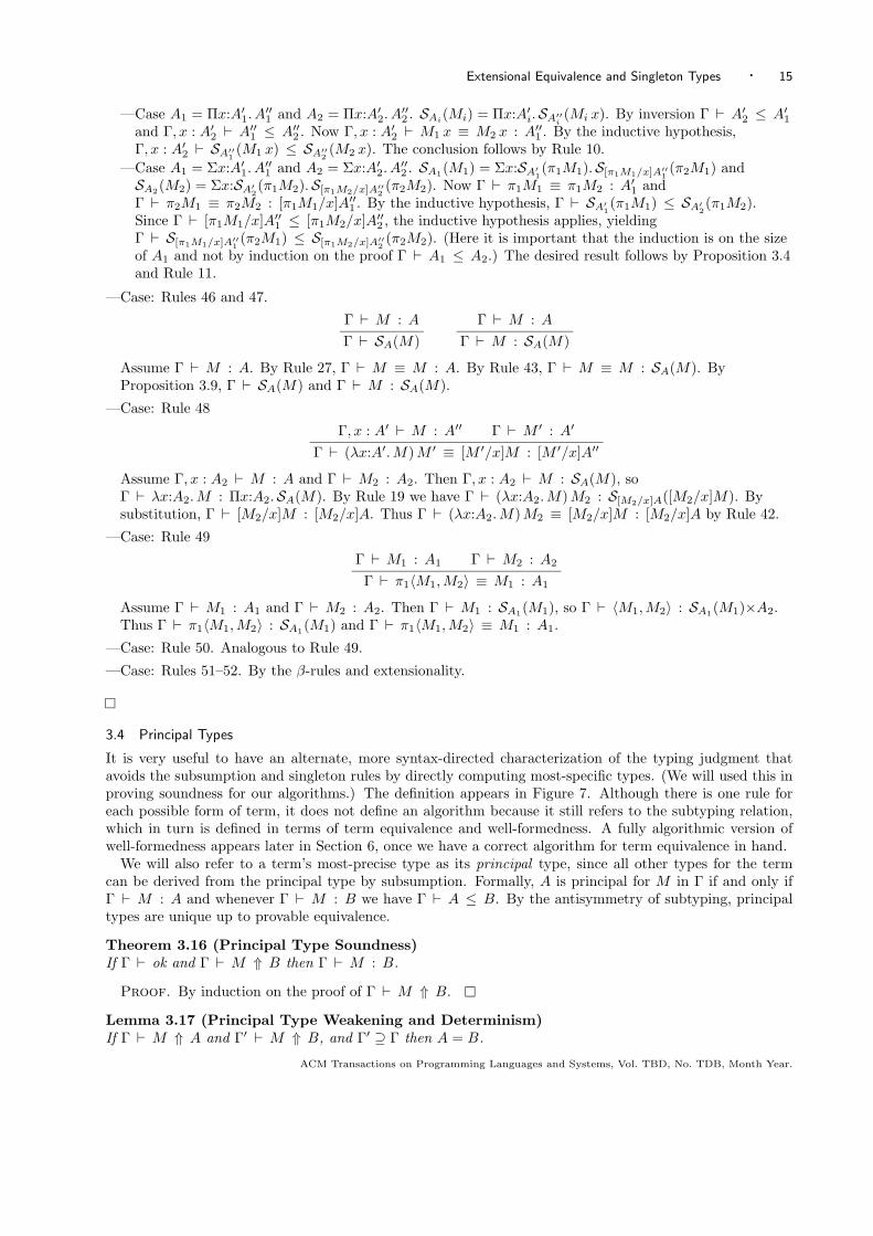
3.4 Principal Types

It is very useful to have an alternate, more syntax-directed characterization of the typing judgment thatavoids the subsumption and singleton rules by directly computing most-specific types. (We will used this inproving soundness for our algorithms.) The definition appears in Figure 7. Although there is one rule foreach possible form of term, it does not define an algorithm because it still refers to the subtyping relation,which in turn is defined in terms of term equivalence and well-formedness. A fully algorithmic version ofwell-formedness appears later in Section 6, once we have a correct algorithm for term equivalence in hand.

We will also refer to a term’s most-precise type as its principal type, since all other types for the termcan be derived from the principal type by subsumption. Formally, A is principal for M in Γ if and only ifΓ ` M : A and whenever Γ ` M : B we have Γ ` A ≤ B. By the antisymmetry of subtyping, principaltypes are unique up to provable equivalence.

Theorem 3.16 (Principal Type Soundness)If Γ ` ok and Γ ` M ⇑ B then Γ ` M : B.

Proof. By induction on the proof of Γ ` M ⇑ B.

Lemma 3.17 (Principal Type Weakening and Determinism)If Γ ` M ⇑ A and Γ′ ` M ⇑ B, and Γ′ ⊇ Γ then A = B.



Γ ` c ⇑ S(c)Γ ` x ⇑ SΓ(x)(x)

Γ ` λx:A′.M ⇑ Πx:A′. A′′ if Γ ` A′ and x 6∈ dom(Γ) and Γ, x : A′ ` M ⇑ A′′Γ ` MM ′ ⇑ [M ′/x]A′′ if Γ ` M ⇑ Πx:A′. A′′ and Γ ` M ′ ⇑ A′1 and Γ ` A′1 ≤ A′

Γ ` 〈M ′,M ′′〉 ⇑ A′×A′′ if Γ ` M ′ ⇑ A′ and Γ ` M ′′ ⇑ A′′.Γ ` π1M ⇑ A′ if Γ ` M ⇑ A′×A′′Γ ` π2M ⇑ A′′ if Γ ` M ⇑ A′×A′′

Fig. 7. Rules for Principal Types

Theorem 3.18 (Principal Type Completeness)If Γ ` M : B then there exists A (determined by Γ and M) such that Γ ` M ⇑ A and Γ ` A ≤ SB(M)(so that Γ ` A ≤ B).

Proof. By induction on the proof of the assumption and cases on the last rule used. The idea ofreplacing the general subsumption rule with a single use of subtyping within applications is very common,so we show only a few cases involving rules specific to λΠΣS

≤ .

—Case: Rule 23Γ ` M : b

Γ ` M : S(M)

By the inductive hypothesis, noting that SS(M)(M) = S(M). (It is important here that the inductionhypothesis guarantees A ≤ SB(M) rather than just A ≤ B.)

—Case: Rule 24.Γ ` Σx:B′. B′′

Γ ` π1M : B′ Γ ` π2M : [π1M/x]B′′

Γ ` M : Σx:B′. B′′

By the inductive hypothesis, Γ ` π1M ⇑ A′and Γ ` A′ ≤ SB′(π1M). Similarly, Γ ` π2M ⇑ A′′ andΓ ` A′′ ≤ S[π1M/x]B′′(π2M). By inversion of the principal type rules, and the observation that theycannot produce a dependent Σ type, it must be that Γ ` M ⇑ A′×A′′. SinceSΣx:B′. B′′(M) = SB′(π1M)×S[π1M/x]B′′(π2M), by Rule 11 and Prop 3.4 we haveΓ ` A′×A′′ ≤ SΣx:B′. B′′(M).

—Case: Rule 25Γ, x : B′ ` M x : B′′

Γ ` M : Πx:B′. B2′′ Γ ` Πx:B′. B2

′′

Γ ` M : Πx:B′. B′′

By the inductive hypothesis, Γ ` M ⇑ A, Γ ` M : A, and Γ ` A ≤ SΠx:B′. B′′2(M). Now

SΠx:B′. B′′2(M) = Πx:B′.SB′′2 (M x) so by inversion of Rule 10, A = Πx:A′. A′′ and Γ ` B′ ≤ A′. Also by

the inductive hypothesis, Γ, x : B′ ` M x ⇑ A′′2 , Γ, x : B′ ` M x : A′′2 , and Γ, x : B′ ` A′′2 ≤ SB′′(M x).But by Lemma 3.17 we have A′′2 = [x/x]A′′ = A′′. Now SΠx:B′. B′′(M) = Πx:B′.SB′′(M x). ThereforeΓ ` Πx:A′. A′′ ≤ SΠx:B′. B′′(M).

4. NORMALIZATION OF TERMS AND TYPES

4.1 Introduction

Determining whether types and types are well-formed is straightforward once we have a method for checkingequivalence of well-formed type terms. The fact that equivalence is sensitive both to the typing context andto the classifying type makes it difficult to use context-insensitive rewrite rules such as the usual β-reductions.We therefore introduce a complete algorithm for computing the normal form of a term given a context anda type; two terms are then provably equivalent if and only if they have the same normal form. (In Section 6we use the correctness of normalization to show the correctness of a more efficient method of determiningtype equivalence.)ACM Transactions on Programming Languages and Systems, Vol. TBD, No. TDB, Month Year.


Natural TypesΓ . c ↑ bΓ . x ↑ Γ(x)Γ . π1p ↑ A′ if Γ . p ↑ Σy:A′. A′′

Γ . π2p ↑ [π1p/y]A′′ if Γ . p ↑ Σy:A′. A′′

Γ . pM ↑ [M/y]A′′ if Γ . p ↑ Πy:A′. A′′

Head ReductionΓ . E[(λx:A.M)M ′] ; E[[M ′/x]M ]Γ . E[π1〈M1,M2〉] ; E[M1]

Γ . E[π2〈M1,M2〉] ; E[M2]Γ . E[p] ; E[N ] if Γ . p ↑ S(N)

Head NormalizationΓ . M ⇓ N if Γ . M ; M ′ and Γ . M ′ ⇓ NΓ . M ⇓M otherwise

Term NormalizationΓ . M : b =⇒M ′′ if Γ . M ⇓M ′ and Γ . M ′ −→M ′′ ↑ bΓ . M : S(N) =⇒M ′′ if Γ . M ⇓M ′ and Γ . M ′ −→M ′′ ↑ bΓ . M : Πx:A′. A′′ =⇒ λx:B′. N if Γ . A′ =⇒ B′ and Γ, x : A′ . (M x) : A′′ =⇒ N

Γ . M : Σx:A′. A′′ =⇒ 〈N ′, N ′′〉 if Γ . π1M : A′ =⇒ N ′ and Γ . π2M : [π1M/x]A′′ =⇒ N ′′.

Path Normalization

Γ . c −→ c ↑ bΓ . x −→ x ↑ Γ(x)Γ . pM −→ p′M ′ ↑ [M/x]A′′ if Γ . p −→ p′ ↑ Πx:A′. A′′ and Γ . M : A′ =⇒M ′

Γ . π1p −→ π1p′ ↑ A′ if Γ . p −→ p′ ↑ Σx:A′. A′′

Γ . π2p −→ π2p′ ↑ [π1p/x]A′ if Γ . p −→ p′ ↑ Σx:A′. A′′

Type NormalizationΓ . b =⇒ b

Γ . S(M) =⇒ S(M ′) if Γ . M : b =⇒M ′

Γ .Πx:A′. A′′ =⇒ Πx:B.B′′ if Γ . A′ =⇒ B′ and Γ, x : A′ . A′′ =⇒ B′′

Γ . Σx:A′. A′′ =⇒ Σx:B.B′′ if Γ . A′ =⇒ B′ and Γ, x : A′ . A′′ =⇒ B′′

Fig. 8. Normalization Algorithm

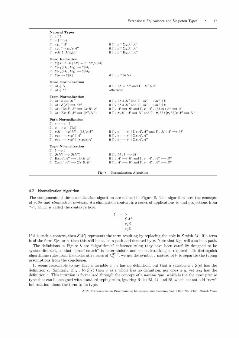
4.2 Normalization Algorithm

The components of the normalization algorithm are defined in Figure 8. The algorithm uses the conceptsof paths and elimination contexts. An elimination context is a series of applications to and projections from“�”, which is called the context’s hole.

E ::= �| EM| π1E| π2E

If E is such a context, then E [M ] represents the term resulting by replacing the hole in E with M . If a termis of the form E [x] or ci then this will be called a path and denoted by p. Note that E [p] will also be a path.

The definitions in Figure 8 are “algorithmic” inference rules; they have been carefully designed to besyntax-directed, so that “proof search” is deterministic and no backtracking is required. To distinguishalgorithmic rules from the declarative rules of λΠΣS

≤ , we use the symbol . instead of ` to separate the typingassumptions from the conclusion.

It seems reasonable to say that a variable x : b has no definition, but that a variable x : S(c) has thedefinition c. Similarly, if y : b×S(c) then y as a whole has no definition, nor does π1y, yet π2y has thedefinition c. This intuition is formalized through the concept of a natural type, which is the the most precisetype that can be assigned with standard typing rules, ignoring Rules 23, 24, and 25, which cannot add “new”information about the term to its type.



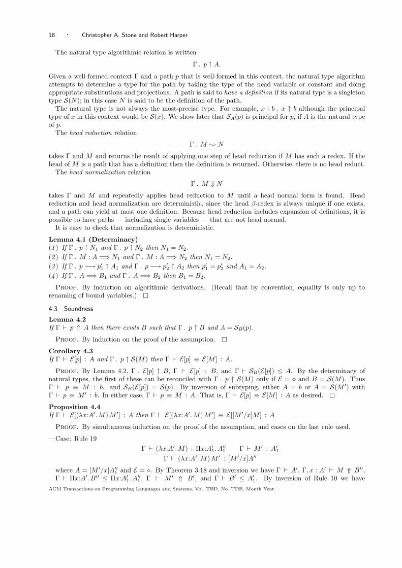
The natural type algorithmic relation is written

Γ . p ↑ A.

Given a well-formed context Γ and a path p that is well-formed in this context, the natural type algorithmattempts to determine a type for the path by taking the type of the head variable or constant and doingappropriate substitutions and projections. A path is said to have a definition if its natural type is a singletontype S(N); in this case N is said to be the definition of the path.

The natural type is not always the most-precise type. For example, x : b . x ↑ b although the principaltype of x in this context would be S(x). We show later that SA(p) is principal for p, if A is the natural typeof p.

The head reduction relation

Γ . M ; N

takes Γ and M and returns the result of applying one step of head reduction if M has such a redex. If thehead of M is a path that has a definition then the definition is returned. Otherwise, there is no head reduct.

The head normalization relation

Γ . M ⇓ N

takes Γ and M and repeatedly applies head reduction to M until a head normal form is found. Headreduction and head normalization are deterministic, since the head β-redex is always unique if one exists,and a path can yield at most one definition. Because head reduction includes expansion of definitions, it ispossible to have paths — including single variables — that are not head normal.

It is easy to check that normalization is deterministic.

Lemma 4.1 (Determinacy)(1 ) If Γ . p ↑ N1 and Γ . p ↑ N2 then N1 = N2.(2 ) If Γ . M : A =⇒ N1 and Γ . M : A =⇒ N2 then N1 = N2.(3 ) If Γ . p −→ p′1 ↑ A1 and Γ . p −→ p′2 ↑ A2 then p′1 = p′2 and A1 = A2.(4 ) If Γ . A =⇒ B1 and Γ . A =⇒ B2 then B1 = B2.

Proof. By induction on algorithmic derivations. (Recall that by convention, equality is only up torenaming of bound variables.)

4.3 Soundness

Lemma 4.2If Γ ` p ⇑ A then there exists B such that Γ . p ↑ B and A = SB(p).

Proof. By induction on the proof of the assumption.

Corollary 4.3If Γ ` E [p] : A and Γ . p ↑ S(M) then Γ ` E [p] ≡ E [M ] : A.

Proof. By Lemma 4.2, Γ . E [p] ↑ B, Γ ` E [p] : B, and Γ ` SB(E [p]) ≤ A. By the determinacy ofnatural types, the first of these can be reconciled with Γ . p ↑ S(M) only if E = � and B = S(M). ThusΓ ` p ≡ M : b. and SB(E [p]) = S(p). By inversion of subtyping, either A = b or A = S(M ′) withΓ ` p ≡ M ′ : b. In either case, Γ ` p ≡ M : A. That is, Γ ` E [p] ≡ E [M ] : A as desired.

Proposition 4.4If Γ ` E [(λx:A′.M)M ′] : A then Γ ` E [(λx:A′.M)M ′] ≡ E [[M ′/x]M ] : A

Proof. By simultaneous induction on the proof of the assumption, and cases on the last rule used.

—Case: Rule 19Γ ` (λx:A′.M) : Πx:A′1. A

′′1 Γ ` M ′ : A′1

Γ ` (λx:A′.M)M ′ : [M ′/x]A′′

where A = [M ′/x]A′′1 and E = �. By Theorem 3.18 and inversion we have Γ ` A′, Γ, x : A′ ` M ⇑ B′′,Γ ` Πx:A′. B′′ ≤ Πx:A′1. A

′′1 , Γ ` M ′ ⇑ B′, and Γ ` B′ ≤ A′1. By inversion of Rule 10 we have



Γ ` A′1 ≤ A′ and Γ, x : A′1 ` B′′ ≤ A′′1 . By Theorem 3.16 we have Γ, x : A′ ` M : B′′ and by subsump-tion Γ ` M ′ : A′, so by Rule 48 we have Γ ` (λx:A′.M)M ′ ≡ [M ′/x]M : [M ′/x]B′′. By Proposition 3.6Γ ` [M ′/x]B′′ ≤ [M ′/x]A′′1 , so by subsumption we have Γ ` (λx:A′.M)M ′ ≡ [M ′/x]M : [M ′/x]A′′1

—Case: Rule 23.

Γ ` E [(λx:A′.M)M ′] : bΓ ` E [(λx:A′.M)M ′] : S(E [(λx:A′.M)M ′])

By induction we have Γ ` E [(λx:A′.M)M ′] ≡ E [[M ′/x]M ] : b. By Rules 28 and 40 we have Γ `E [[M ′/x]M ] ≡ E [(λx:A′.M)M ′] : S(E [(λx:A′.M)M ′]), so the desired result follows by another applica-tion of Rule 28.

—The remaining cases follow similarly by induction.

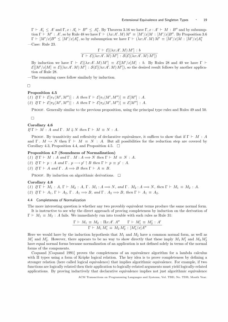
Proposition 4.5(1 ) If Γ ` E [π1〈M ′,M ′′〉] : A then Γ ` E [π1〈M ′,M ′′〉] ≡ E [M ′] : A.(2 ) If Γ ` E [π2〈M ′,M ′′〉] : A then Γ ` E [π2〈M ′,M ′′〉] ≡ E [M ′′] : A.

Proof. Generally similar to the previous proposition, using the principal type rules and Rules 49 and 50.

Corollary 4.6If Γ ` M : A and Γ . M ⇓ N then Γ ` M ≡ N : A.

Proof. By transitivity and reflexivity of declarative equivalence, it suffices to show that if Γ ` M : Aand Γ . M ; N then Γ ` M ≡ N : A. But all possibilities for the reduction step are covered byCorollary 4.3, Proposition 4.4, and Proposition 4.5.

Proposition 4.7 (Soundness of Normalization)(1 ) If Γ ` M : A and Γ . M : A =⇒ N then Γ ` M ≡ N : A.(2 ) If Γ ` p : A and Γ . p −→ p′ ↑ B then Γ ` p ≡ p′ : A.(3 ) If Γ ` A and Γ . A =⇒ B then Γ ` A ≡ B.

Proof. By induction on algorithmic derivations.

Corollary 4.8(1 ) If Γ ` M1 : A, Γ ` M2 : A, Γ . M1 : A =⇒ N , and Γ . M2 : A =⇒ N , then Γ ` M1 ≡ M2 : A.(2 ) If Γ ` A1, Γ ` A2, Γ . A1 =⇒ B, and Γ . A2 =⇒ B, then Γ ` A1 ≡ A2.

4.4 Completeness of Normalization

The more interesting question is whether any two provably equivalent terms produce the same normal form.It is instructive to see why the direct approach of proving completeness by induction on the derivation of

Γ ` M1 ≡ M2 : A fails. We immediately run into trouble with such rules as Rule 31:

Γ ` M1 ≡ M2 : Πx:A′. A′′ Γ ` M ′1 ≡ M ′2 : A′

Γ ` M1M′1 ≡ M2M

′2 : [M ′1/x]A′′

Here we would have by the induction hypothesis that M1 and M2 have a common normal form, as well asM ′1 and M ′2. However, there appears to be no way to show directly that these imply M1M

′1 and M2M

′2

have equal normal forms because normalization of an application is not defined solely in terms of the normalforms of the components.

Coquand [Coquand 1991] proves the completeness of an equivalence algorithm for a lambda calculuswith Π types using a form of Kripke logical relation. The key idea is to prove completeness by defining astronger relation (here called logical equivalence) that implies algorithmic equivalence. For example, if twofunctions are logically related then their application to logically-related arguments must yield logically-relatedapplications. By proving inductively that declarative equivalence implies not just algorithmic equivalence



but logical equivalence, we have strengthened the induction hypothesis enough to allow cases such as Rule 31to go through.

To show the completeness and termination for the algorithm we use a modified Kripke-style logical relationsargument. The primary difficulty is the context-sensitive nature of normalization, which makes it difficultto define a natural logical equivalence relation that guarantees common normal forms. For example, if wehave two type terms M and N of type Σx:A′. A′′ then a natural definition of a binary logical equivalencerelation would require both that π1M and π1N are logically equivalent at type A′, and that π2M andπ2N are logically equivalent. But at what type should the latter pair be compared? The most obviouschoices are (the declaratively equivalent, but a priori not algorithmically equivalent) types [π1M/x]A′′ or[π1N/x]A′′. But even if we were to require that π2M and π2N be logically equivalent at both types, thisappears insufficient to guarantee that M and N have equal normal forms: normalizing M and N at the typeΣx:A′. A′′ will involve normalizing π2M at type [π1M/x]A′′ and normalizing π2N at type [π1N/x]A′′. If thelogical relation guarantees only that for any fixed type the two projections have the same normal form, thisis not enough.2

We therefore move to a formulation that allows us to express the fact that multiple terms considered atmultiple types and in multiple contexts should all have a single common normal form. Our Kripke world ∆is a nonempty set of contexts. The preorder � is defined as follow:

∆1 � ∆2 :⇐⇒ ∀θ2 ∈ ∆2.∃θ1 ∈ ∆1.θ1 ⊆ θ2.

where ⊆ is the subset ordering on contexts. That is, if ∆1 � ∆2 then every context in ∆2 extends somecontext in ∆1.

Similarly we will use A and L to range over finite, non-empty sets of types,M and N to range over finite,non-empty sets of terms, and G to range over finite, non-empty sets of substitutions.

It turns out to be very convenient to define notation using sets of types where one would normally use asingle type, and sets of type terms where one would normally use a single term, with the result being a setcomputed pointwise:

[M/x]A := { [M/x]A | M ∈M }[M/x]A := { [M/x]A | M ∈M, A ∈ A}MM′ := { MM ′ | M ∈M,M ′ ∈M′}πiM := { πiM | M ∈M }G(M) := { γ(M) | γ ∈ G }G(A) := { γ(A) | γ ∈ G, A ∈ A }dom(G) :=

⋃{ dom(γ) | γ ∈ G }

rng(G) :=⋃{ rng(γ) | γ ∈ G }

S(M) := { S(M) | M ∈M }

If A is a set { Πx:A′i. A′′i | i ∈ I }, it is also very convenient to define a form of pattern-matching where

we write “A = Πx:A′.A′′” to mean that A′ = { A′i | i ∈ I } and A′′ = { A′′i | i ∈ I }. The notationA = Σx:A′.A′′ when A is a set of Σ types is defined analogously.

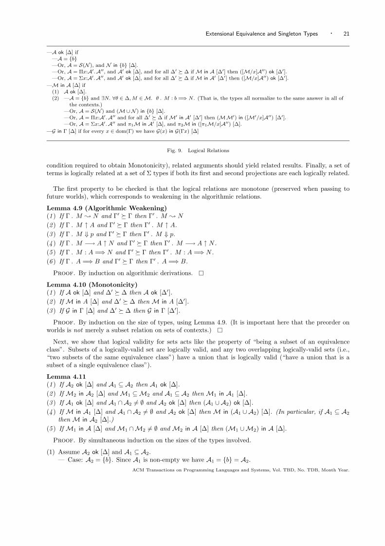
The logical relations are then defined as shown in Figure 9. Logically related sets of types, written A ok [∆],are those which can index our logical relation for sets of terms. All elements of a logically related set of typesmust have the same “shape” (and the same size). In the base case, a set just containing the base type b islogically related, while a set of singleton types are logically related if they have the same normal form in allcontexts in the world. A set of Π kinds is logically related if their domains form a logically related set, andif substitution instances of their codomains are as well. The condition for a set of Σ kinds is similar.

Logical relatedness of a set of terms is defined inductively on the common size of the elements of a logicallyrelated set of types. In the base case, a set of terms of the base type if they have the same normal formunder all contexts in the world. Similarly, a set of terms is logically related with respect to a set of singletontypes if the terms in the set and those in the singletons all have common normal forms. The definition forterms at a set of Π types is the usual Kripke logical relations definition lifted to sets: in all future worlds (a

2Modifying the algorithm to substitute in the normal form of π1M would resolve this problem, but then require that we provea term and its fully normalized form are logically equivalent, which does not appear directly provable.



—A ok [∆] if—A = {b}—Or, A = S(N ), and N in {b} [∆].—Or, A = Πx:A′.A′′, and A′ ok [∆], and for all ∆′ � ∆ if M in A [∆′] then ([M/x]A′′) ok [∆′].—Or, A = Σx:A′.A′′, and A′ ok [∆], and for all ∆′ � ∆ if M in A′ [∆′] then ([M/x]A′′) ok [∆′].

—M in A [∆] if(1) A ok [∆].

(2) —A = {b} and ∃N. ∀θ ∈ ∆,M ∈M. θ . M : b =⇒ N . (That is, the types all normalize to the same answer in all ofthe contexts.)

—Or, A = S(N ) and (M∪N ) in {b} [∆].

—Or, A = Πx:A′.A′′ and for all ∆′ � ∆ if M′ in A′ [∆′] then (MM′) in ([M′/x]A′′) [∆′].—Or, A = Σx:A′.A′′ and π1M in A′ [∆], and π2M in ([π1M/x]A′′) [∆].

—G in Γ [∆] if for every x ∈ dom(Γ) we have G(x) in G(Γx) [∆]

Fig. 9. Logical Relations

condition required to obtain Monotonicity), related arguments should yield related results. Finally, a set ofterms is logically related at a set of Σ types if both its first and second projections are each logically related.

The first property to be checked is that the logical relations are monotone (preserved when passing tofuture worlds), which corresponds to weakening in the algorithmic relations.

Lemma 4.9 (Algorithmic Weakening)(1 ) If Γ . M ; N and Γ′ � Γ then Γ′ . M ; N

(2 ) If Γ . M ↑ A and Γ′ � Γ then Γ′ . M ↑ A.(3 ) If Γ . M ⇓ p and Γ′ � Γ then Γ′ . M ⇓ p.(4 ) If Γ . M −→ A ↑ N and Γ′ � Γ then Γ′ . M −→ A ↑ N .(5 ) If Γ . M : A =⇒ N and Γ′ � Γ then Γ′ . M : A =⇒ N .(6 ) If Γ . A =⇒ B and Γ′ � Γ then Γ′ . A =⇒ B.

Proof. By induction on algorithmic derivations.

Lemma 4.10 (Monotonicity)(1 ) If A ok [∆] and ∆′ � ∆ then A ok [∆′].(2 ) If M in A [∆] and ∆′ � ∆ then M in A [∆′].(3 ) If G in Γ [∆] and ∆′ � ∆ then G in Γ [∆′].

Proof. By induction on the size of types, using Lemma 4.9. (It is important here that the preorder onworlds is not merely a subset relation on sets of contexts.)

Next, we show that logical validity for sets acts like the property of “being a subset of an equivalenceclass”. Subsets of a logically-valid set are logically valid, and any two overlapping logically-valid sets (i.e.,“two subsets of the same equivalence class”) have a union that is logically valid (“have a union that is asubset of a single equivalence class”).

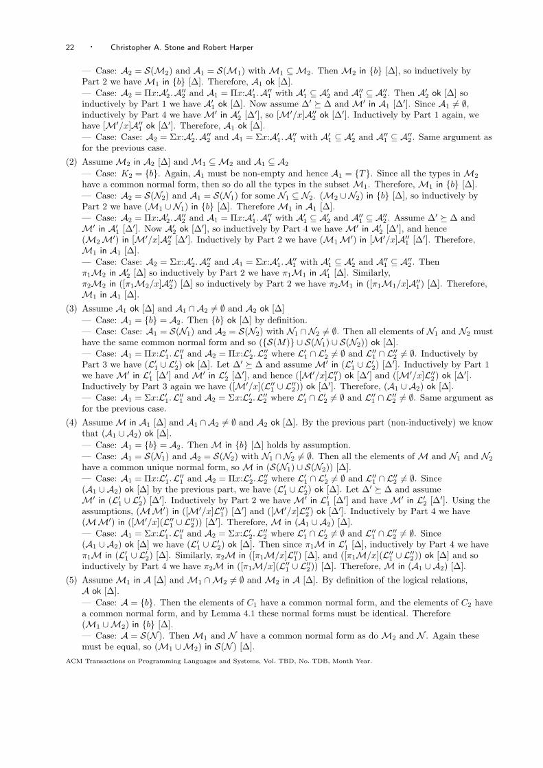
Lemma 4.11(1 ) If A2 ok [∆] and A1 ⊆ A2 then A1 ok [∆].(2 ) If M2 in A2 [∆] and M1 ⊆M2 and A1 ⊆ A2 then M1 in A1 [∆].(3 ) If A1 ok [∆] and A1 ∩ A2 6= ∅ and A2 ok [∆] then (A1 ∪ A2) ok [∆].(4 ) If M in A1 [∆] and A1 ∩ A2 6= ∅ and A2 ok [∆] then M in (A1 ∪ A2) [∆]. (In particular, if A1 ⊆ A2

then M in A2 [∆].)(5 ) If M1 in A [∆] and M1 ∩M2 6= ∅ and M2 in A [∆] then (M1 ∪M2) in A [∆].

Proof. By simultaneous induction on the sizes of the types involved.

(1) Assume A2 ok [∆] and A1 ⊆ A2.— Case: A2 = {b}. Since A1 is non-empty we have A1 = {b} = A2.



— Case: A2 = S(M2) and A1 = S(M1) with M1 ⊆M2. Then M2 in {b} [∆], so inductively byPart 2 we have M1 in {b} [∆]. Therefore, A1 ok [∆].— Case: A2 = Πx:A′2.A′′2 and A1 = Πx:A′1.A′′1 with A′1 ⊆ A′2 and A′′1 ⊆ A′′2 . Then A′2 ok [∆] soinductively by Part 1 we have A′1 ok [∆]. Now assume ∆′ � ∆ and M′ in A1 [∆′]. Since A1 6= ∅,inductively by Part 4 we have M′ in A′2 [∆′], so [M′/x]A′′2 ok [∆′]. Inductively by Part 1 again, wehave [M′/x]A′′1 ok [∆′]. Therefore, A1 ok [∆].— Case: Case: A2 = Σx:A′2.A′′2 and A1 = Σx:A′1.A′′1 with A′1 ⊆ A′2 and A′′1 ⊆ A′′2 . Same argument asfor the previous case.

(2) Assume M2 in A2 [∆] and M1 ⊆M2 and A1 ⊆ A2

— Case: K2 = {b}. Again, A1 must be non-empty and hence A1 = {T}. Since all the types in M2

have a common normal form, then so do all the types in the subset M1. Therefore, M1 in {b} [∆].— Case: A2 = S(N2) and A1 = S(N1) for some N1 ⊆ N2. (M2 ∪N2) in {b} [∆], so inductively byPart 2 we have (M1 ∪N1) in {b} [∆]. Therefore M1 in A1 [∆].— Case: A2 = Πx:A′2.A′′2 and A1 = Πx:A′1.A′′1 with A′1 ⊆ A′2 and A′′1 ⊆ A′′2 . Assume ∆′ � ∆ andM′ in A′1 [∆′]. Now A′2 ok [∆′], so inductively by Part 4 we have M′ in A′2 [∆′], and hence(M2M′) in [M′/x]A′′2 [∆′]. Inductively by Part 2 we have (M1M′) in [M′/x]A′′1 [∆′]. Therefore,M1 in A1 [∆].— Case: Case: A2 = Σx:A′2.A′′2 and A1 = Σx:A′1.A′′1 with A′1 ⊆ A′2 and A′′1 ⊆ A′′2 . Thenπ1M2 in A′2 [∆] so inductively by Part 2 we have π1M1 in A′1 [∆]. Similarly,π2M2 in ([π1M2/x]A′′2) [∆] so inductively by Part 2 we have π2M1 in ([π1M1/x]A′′1) [∆]. Therefore,M1 in A1 [∆].

(3) Assume A1 ok [∆] and A1 ∩ A2 6= ∅ and A2 ok [∆]— Case: A1 = {b} = A2. Then {b} ok [∆] by definition.— Case: Case: A1 = S(N1) and A2 = S(N2) with N1 ∩N2 6= ∅. Then all elements of N1 and N2 musthave the same common normal form and so ({S(M)} ∪ S(N1) ∪ S(N2)) ok [∆].— Case: A1 = Πx:L′1.L′′1 and A2 = Πx:L′2.L′′2 where L′1 ∩ L′2 6= ∅ and L′′1 ∩ L′′2 6= ∅. Inductively byPart 3 we have (L′1 ∪ L′2) ok [∆]. Let ∆′ � ∆ and assume M′ in (L′1 ∪ L′2) [∆′]. Inductively by Part 1we have M′ in L′1 [∆′] and M′ in L′2 [∆′], and hence ([M′/x]L′′1) ok [∆′] and ([M′/x]L′′2) ok [∆′].Inductively by Part 3 again we have ([M′/x](L′′1 ∪ L′′2)) ok [∆′]. Therefore, (A1 ∪ A2) ok [∆].— Case: A1 = Σx:L′1.L′′1 and A2 = Σx:L′2.L′′2 where L′1 ∩ L′2 6= ∅ and L′′1 ∩ L′′2 6= ∅. Same argument asfor the previous case.

(4) Assume M in A1 [∆] and A1 ∩A2 6= ∅ and A2 ok [∆]. By the previous part (non-inductively) we knowthat (A1 ∪ A2) ok [∆].— Case: A1 = {b} = A2. Then M in {b} [∆] holds by assumption.— Case: A1 = S(N1) and A2 = S(N2) with N1 ∩N2 6= ∅. Then all the elements of M and N1 and N2

have a common unique normal form, so M in (S(N1) ∪ S(N2)) [∆].— Case: A1 = Πx:L′1.L′′1 and A2 = Πx:L′2.L′′2 where L′1 ∩ L′2 6= ∅ and L′′1 ∩ L′′2 6= ∅. Since(A1 ∪ A2) ok [∆] by the previous part, we have (L′1 ∪ L′2) ok [∆]. Let ∆′ � ∆ and assumeM′ in (L′1 ∪ L′2) [∆′]. Inductively by Part 2 we have M′ in L′1 [∆′] and have M′ in L′2 [∆′]. Using theassumptions, (MM′) in ([M′/x]L′′1) [∆′] and ([M′/x]L′′2) ok [∆′]. Inductively by Part 4 we have(MM′) in ([M′/x](L′′1 ∪ L′′2)) [∆′]. Therefore, M in (A1 ∪ A2) [∆].— Case: A1 = Σx:L′1.L′′1 and A2 = Σx:L′2.L′′2 where L′1 ∩ L′2 6= ∅ and L′′1 ∩ L′′2 6= ∅. Since(A1 ∪ A2) ok [∆] we have (L′1 ∪ L′2) ok [∆]. Then since π1M in L′1 [∆], inductively by Part 4 we haveπ1M in (L′1 ∪ L′2) [∆]. Similarly, π2M in ([π1M/x]L′′1) [∆], and ([π1M/x](L′′1 ∪ L′′2)) ok [∆] and soinductively by Part 4 we have π2M in ([π1M/x](L′′1 ∪ L′′2)) [∆]. Therefore, M in (A1 ∪ A2) [∆].

(5) Assume M1 in A [∆] and M1 ∩M2 6= ∅ and M2 in A [∆]. By definition of the logical relations,A ok [∆].— Case: A = {b}. Then the elements of C1 have a common normal form, and the elements of C2 havea common normal form, and by Lemma 4.1 these normal forms must be identical. Therefore(M1 ∪M2) in {b} [∆].— Case: A = S(N ). Then M1 and N have a common normal form as do M2 and N . Again thesemust be equal, so (M1 ∪M2) in S(N ) [∆].



— Case: A = Πx:A′.A′′. Assume ∆′ � ∆ and M′ in A′ [∆′]. Then (M1M′) in ([M′/x]A′′) [∆′] and(M2M′) in ([M′/x]A′′) [∆′]. Since M′ 6= ∅, (M1M′)∩ (M2M′) 6= ∅ and hence inductively by Part 5we have ((M1 ∪M2)M′) in ([M′/x]A′′) [∆′]. Therefore, (M1 ∪M2) in A [∆].— Case: A = Σx:A′.A′′. Then π1M1 in A′ [∆] and π1M2 in A′ [∆] and these two sets of termsoverlap, so inductively by Part 5 we have π1(M1 ∪M2) in A′ [∆]. Next, we haveπ2M1 in ([π1M1/x]A′′) [∆] and π2M2 in ([π1M2/x]A′′) [∆] and ([π1(M1 ∪M2)/x]A′′) ok [∆], soinductively by Parts 4 and 5 we have π2(M1 ∪M2) in ([π1(M1 ∪M2)/x]A′′) [∆]. Therefore,(M1 ∪M2) in A [∆].

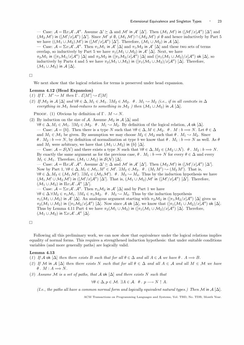
We next show that the logical relation for terms is preserved under head expansion.

Lemma 4.12 (Head Expansion)(1 ) If Γ . M ′ ; M then Γ . E [M ′] ; E [M ](2 ) If M2 in A [∆] and ∀θ ∈ ∆,M1 ∈M1. ∃M2 ∈M2. θ . M1 ; M2 (i.e., if in all contexts in ∆

everything in M1 head-reduces to something in M2 ) then (M1 ∪M2) in A [∆].

Proof. (1) Obvious by definition of Γ . M ; N .(2) By induction on the size of A. Assume M2 in A [∆] and∀θ ∈ ∆,M1 ∈M1. ∃M2 ∈M2. θ . M1 ; M2. By definition of the logical relation, A ok [∆].— Case: A = {b}. Then there is a type N such that ∀θ ∈ ∆,M ∈M2. θ . M : b =⇒ N . Let θ ∈ ∆and M1 ∈M1 be given. By assumption we may choose M2 ∈M2 such that θ . M1 ; M2. Sinceθ . M2 : b =⇒ N , by definition of normalization at type b we know that θ . M1 : b =⇒ N as well. As θand M1 were arbitrary, we have that (M1 ∪M2) in {b} [∆].— Case: A = S(N ) and there exists a type N such that ∀θ ∈ ∆,M2 ∈ (M2 ∪N ). θ . M2 : b =⇒ N .By exactly the same argument as for the previous case, θ . M1 : b =⇒ N for every θ ∈ ∆ and everyM1 ∈M1. Therefore, (M1 ∪M2) in S(N ) [∆].— Case: A = Πx:A′.A′′. Assume ∆′ � ∆ and M′ in A′ [∆′]. Then (M2M′) in ([M′/x]A′′) [∆′].Now by Part 1, ∀θ ∈ ∆,M1 ∈M1,M

′ ∈M′. ∃M2 ∈M2. θ . (M1M′) ; (M2M

′). That is,∀θ ∈ ∆,M3 ∈ (M1M′). ∃M4 ∈ (M2M′). θ . M3 ; M4. Thus by the induction hypothesis we have(M1M′ ∪M2M′) in ([M′/x]A′′) [∆′]. That is, (M1 ∪M2)M′ in ([M′/x]A′′) [∆′]. Therefore,(M1 ∪M2) in Πx:A′.A′′ [∆′].— Case: A = Σx:A′.A′′. Then π1M2 in A′ [∆] and by Part 1 we have∀θ ∈ ∆.∀M3 ∈ π1M1. ∃M4 ∈ π1M2. θ . M3 ; M4. Thus by the induction hypothesisπ1(M1 ∪M2) in A′ [∆]. An analogous argument starting with π2M2 in ([π1M2/x]A′′) [∆] gives usπ2(M1 ∪M2) in ([π1M2/x]A′′) [∆]. Now since A ok [∆], we know that ([π1(M1 ∪M2)/x]A′′) ok [∆].Thus by Lemma 4.11 Part 4 we have π2(M1 ∪M2) in ([π1(M1 ∪M2)/x]A′′) [∆]. Therefore,(M1 ∪M2) in Σx:A′.A′′ [∆].

Following all this preliminary work, we can now show that equivalence under the logical relations impliesequality of normal forms. This requires a strengthened induction hypothesis: that under suitable conditionsvariables (and more generally paths) are logically valid.

Lemma 4.13(1 ) If A ok [∆] then there exists B such that for all θ ∈ ∆ and all A ∈ A we have θ . A =⇒ B.(2 ) If M in A [∆] then there exists N such that for all θ ∈ ∆ and all A ∈ A and all M ∈ M we have

θ . M : A =⇒ N .(3 ) Assume M is a set of paths, that A ok [∆] and there exists N such that

∀θ ∈ ∆, p ∈M. ∃A ∈ A. θ . p −→ N ↑ A.

(I.e., the paths all have a common normal form and logically equivalent natural types.) ThenM in A [∆].



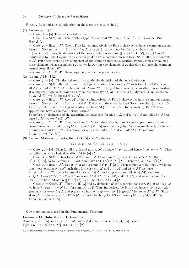
Proof. By simultaneous induction on the sizes of the types in A.

(1) Assume A ok [∆]— Case: A = {b} Then we can take B := b.— Case: A = S(N ) and there exists a type N such that ∀θ ∈ ∆,M ∈ N . θ . M : b =⇒ N . PutB := S(N).— Case: A = Πx:A′.A′′. Then A′ ok [∆], so inductively by Part 1 these types have a common normalform B′. Now put ∆′ := { θ, x : A′ | θ ∈ ∆, A′ ∈ A′ }. Inductively by Part 3 we have that{x} in A′ [∆′]. Thus, by definition of the logical relation we have ([x/x]A′′) ok [∆′], i.e., A′′ ok [∆′].Inductively by Part 1 again, the elements of A′′ have a common normal form B′′ in all of the contextsin ∆′. But these contexts are a superset of the contexts that the algorithm would use in normalizingthese elements when normalizing A, so we know that the elements of A therefore all have the commonnormal form Πx:B′. B′′.— Case: A = Σx:A′.A′′. Same argument as for the previous case.

(2) Assume M in A [∆]— Case: A = {b}. The desired result is exactly the definition of the logical relation.— Case: A = S(N ). By definition of the logical relation, there exists N ′ such that for all θ ∈ ∆ andall A ∈ A and all M ∈M we have θ . M : b =⇒ N ′. But by definition of the algorithm, normalizationat a singleton type is the same as normalization at type b, and so this last judgment is equivalent toθ . M : S(N) =⇒ N ′ for every b ∈ N .— Case: A = Πx:A′.A′′. then A′ ok [∆], so inductively by Part 1 these types have a common normalform B′. Now put ∆′ := {θ, x : A′ | θ ∈ ∆, A′ ∈ A′}. Inductively by Part 3 we have that {x} in A′ [∆′].Thus, by definition of the logical relation we have M{x} in A′′ [∆′]. Inductively by Part 2 theseapplications have a common normal form N ′′.Therefore, by definition of the algorithm we have that for all θ ∈ ∆ and all A ∈ A and all M ∈M wehave θ . M : A =⇒ λx:B′. N ′′.— Case: A = Σx:A′.A′′. Then π1M in A′ [∆] so inductively by Part 2 these types have a commonnormal form N ′. Similarly, π2M in ([π1M/x]A′) [∆] so inductively by Part 2 again these types have acommon normal form N ′′. Therefore, for all θ ∈ ∆ and all A ∈ A and all M ∈M we haveθ . M : A =⇒ 〈N ′, N ′′〉.

(3) Assume M is a set of paths, that A ok [∆] and N satisfies

∀θ ∈ ∆, p ∈M. ∃A ∈ A. θ . p −→ N ↑ A.

— Case: A = {b}. Then for all θ ∈ ∆ and all p ∈M we have θ . p ⇓ p, and hence θ . p : b =⇒ N . Thusby definition of the logical relation, M in {b} [∆].— Case: A = S(N ). Then for all θ ∈ ∆ and p ∈M we have θ . p ; N for some N ∈ N . ButN in {b} [∆], so by Lemma 4.12 Part 2 we have (M∪N ) in {b} [∆]. Therefore, M in S(N ) [∆].— Case: A = Πx:A′.A′′. Let ∆′ � ∆ and assume M′ in A′ [∆′]. Then inductively by Part 2 we knowthat there exists a type N ′ such that for every θ ∈ ∆′ and A′ ∈ A′ and M ′ ∈M′ we haveθ . M ′ : A′ =⇒ N ′. Using Lemma 4.9, for all θ ∈ ∆′ and all p ∈M and all M ′ ∈M′, we haveθ . (pM ′) −→ (N N ′) ↑ [M ′/x]A′′ for some A′′ ∈ A′′. Now [M′/x]A′′ ok [θ′], and so inductively byPart 3 we have MM′ in ([M′/x]A′′) [∆′]. Therefore, M in A [∆].— Case: A = Σx:A′.A′′. Then A′ ok [∆] and by definition of the algorithm for every θ ∈ ∆ and p ∈Mwe have θ . π1p −→ π1N ↑ A′ for some A′ ∈ A′. Thus inductively by Part 3 we have π1M in A′ [∆].Similarly, for every θ ∈ ∆ and p ∈M we have θ . π2p −→ π2N ↑ [π1p/x]A′′ for some A′′ ∈ A′′. SinceA ok [∆], we have [π1M/x]A′′ ok [∆], so inductively by Part 3 we have π2M in [π1M/x]A′′ [∆].Therefore, M in A [∆].

One more lemma is used in the Fundamental Theorem:

Lemma 4.14 (Substitution Extension)Assume G in Γ [∆], and Γ, x : A ` ok, and x 6∈ dom(G), and M in G(A) [∆]. Then{γ[x7→M ] | γ ∈ G,M ∈M} in (Γ, x : A) [∆].



Proof. Assume G in Γ [∆], and Γ, x : A ` ok, and x 6∈ dom(G), and M in G(A) [∆], and putG′ := {γ[x7→M ] | γ ∈ G,M ∈M}. Using Propositions 3.1 and 3.2, α 6∈ rng(Γ) and α 6∈ FV(A). Thus for ally ∈ dom(Γ) we have G(y) in G(Γy) [∆], and G′(y) = G(y), and G′(Γy)) = G(Γy), and (Γ, x : A)y = Γy, andhence G′(y) in G′((Γ, x : A)y) [∆]. Now G′(A) = G(A) and by definition G′(x) =M, soG′(x) in G′((Γ, x : A)x) [∆]. Thus for all y ∈ dom(Γ, x : A) we have G′(y) in G′((Γ, x : A)y) [∆]. That is,G′ in (Γ, x : A) [∆].

Finally we come to the Fundamental Theorem of Logical Relations, which relates provable equivalence ofterms to the logical relations.

Theorem 4.15 (Fundamental Theorem)(1 ) If Γ ` A and G in Γ [∆] then G(A) ok [∆].(2 ) If Γ ` A1 ≤ A2 and G in Γ [∆] then G(A1) ok [∆] and G(A2) ok [∆] and if M in G(A1) [∆] thenM in G(A2) [∆].

(3 ) If Γ ` A1 ≡ A2 and G in Γ [∆] then (G(A1) ∪ G(A2)) ok [∆].(4 ) If Γ ` M : A and G in Γ [∆] then G(M) in G(A) [∆](5 ) If Γ ` M1 ≡ M2 : A and G in Γ [∆] then (G(M1) ∪ G(M2)) in G(A) [∆]

Proof. By induction on the hypothesized derivations.

Type Well-formedness Rules: Γ ` A.

— Case: Rule 3, so A = b.Then G(b) = b and {b} ok [∆].— Case: Rule 4, with A = S(M) because Γ ` M : b.By the inductive hypothesis, G(M) in G(b) [∆]. That is, G(M) in {b} [∆]. Therefore G(S(M)) ok [∆].— Case: Rule 5, with A = Πx:A′. A′′ because Γ, x : A′ ` A′′.Without loss of generality, x 6∈ dom(G) ∪ rng(G). By Proposition 3.1, there is a strict subderivationΓ, x : A′ ` ok and by inversion a strict subderivation Γ ` A′. By the inductive hypothesis, G(A′) ok [∆].Let ∆′ � ∆ and assume that M in G(A′) [∆′]. Put G′ := {γ[x7→M ] | γ ∈ G, M ∈M}. By Lemmas 4.10and 4.14 G′ in (Γ, x : A′) [∆′], so by the inductive hypothesis we have G′(A′′) ok [∆′]. That is,[M/x](G(A′′)) ok [∆′]. Therefore, G(Πx:A′. A′′) ok [∆].— Case: Rule 6, with A = Σx:A′. A′′ because Γ, x : A′ ` A′′. Analogous to the previous case.

Subtyping Rules: Γ ` A1 ≤ A2. In all cases, the proofs that G(A1) ok [∆] and G(A2) ok [∆] followessentially as in the proofs for the well-formedness rules.Assume M in G(A1) [∆]. We must show that M in G(A2) [∆].

— Case: Rule 7, with A1 = S(M) and A2 = b.Then M in b [∆] by the definition of the logical relations.— Case: Rule 8. A1 = S(M1) and A2 = S(M2), with Γ ` M1 ≡ M2 : b.By the inductive hypothesis we have (G(M1) ∪ G(M2)) in b [∆]. Thus G(S(M1)) ∪ G(S(M2)) ok [∆]. ByLemma 4.11 Parts 4 and 2 we have M in G(S(M1)) ∪ G(S(M2)) [∆] and hence M in G(S(M2)) [∆] asrequired.— Case: Rule 9, with A1 = A2 = b.Trivial, since G(b) = b.— Case: Rule 10, with A1 = Πx:A′1. A

′′1 and A2 = Πx:A′2. A

′′2 where Γ ` A′2 ≤ A′1 and

Γ, x : A′2 ` A′′1 ≤ A′′2 .Without loss of generality, x 6∈ dom(G) ∪ rng(G). Let ∆′ � ∆ and assume M′ in G(A′2) [∆′]. By theinductive hypothesis, M′ in G(A′1) [∆′]. Hence (MM′) in [M′/x]G(A′′1) [∆′]. That is,(MM′) in G′(A′′1) [∆′] where G′ := {γ[x7→M ] | γ ∈ G, M ∈M}. By Lemma 4.10, Proposition 3.1 andLemma 4.14, G′ in (Γ, x : A′2) [∆′]. By the inductive hypothesis again, (MM′) in G′(A′′2) [∆′]. That is,(MM′) in [M′/x]G(A′′2) [∆′]. Therefore, M in G(Πx:A′2. A

′′2) [∆].



— Case: Rule 11. A1 = Σx:A′1. A′′1 and A2 = Σx:A′2. A

′′2 with Γ ` A′1 ≤ A′2 and Γ, x : A′1 ` A′′1 ≤ A′′2 .

Without loss of generality, x 6∈ dom(G) ∪ rng(G). By the definitions of the logical relations,π1M in G(A′1) [∆]. By the inductive hypothesis, π1M in G(A′2) [∆]. PutG′ := {γ[x7→M ] | γ ∈ G, M ∈ π1M}. By Proposition 3.1 and Lemma 4.14 we have G′ in Γ, x : A′1 [∆]. Nowπ2M in [π1M/x](G(A′′1)) [∆], i.e., π2M in G′(A′′1) [∆]. So, by the inductive hypothesis π2M in G′(A′′2) [∆].That is, π2M in ([π1M/x]G(A2)) [∆]. Therefore, M in G(Σx:A′2. A

′′2) [∆].

Type Equivalence Rules: Γ ` A1 ≡ A2.

— Case: Rule 12. A1 = A2 = b.{b} ok [∆] by definition.— Case: Rule 13. A1 = S(M1) and A2 = S(M2) with Γ ` M1 ≡ M2 : b.By the inductive hypothesis, (G(M1) ∪ G(M2)) in b [∆]. Therefore by definition of the logical relation,(G(S(M1)) ∪ G(S(M2))) ok [∆].— Case: Rule 14. A1 = Πx:A′1. A

′′1 and A2 = Πx:A′2. A

′′2 with Γ ` A′2 ≡ A′1 and Γ, x : A′1 ` A′′1 ≡ A′′2 .

Without loss of generality, x 6∈ dom(G) ∪ rng(G). By the inductive hypothesis, (G(A′1) ∪ G(A′2)) ok [∆]. Let∆′ � ∆ and assumeM in (G(A′1)∪G(A′2)) [∆′]. By Lemma 4.11 Part 2, M in G(A′1) [∆′]. By Lemma 4.10,Proposition 3.1 and Lemma 4.14, then, G′ in (Γ, x : A′1) [∆′] where G′ := {γ[x7→M ] | γ ∈ G, M ∈M}. Bythe inductive hypothesis again, (G′(A′′1) ∪ G′(A′′2)) ok [∆]. That is, [M′/x](G(A′′1) ∪ G(A′′2)) ok [∆].Therefore, (G(Πx:A′1. A

′′1) ∪ G(Πx:A′2. A

′′2)) ok [∆].

— Case: Rule 15. Same proof as for previous case.

Term Validity Rules Γ ` M : A.

— Case: Rule 16. M = c and A = b. Then {b} ok [∆] and θ . c −→ c ↑ b for every θ ∈ ∆. Thus byLemma 4.13 Part 3 we have {c} in b [∆].— Case: Rule 17. M = x and A = Γx.By assumption, G(x) in G(Γx) [∆].— Case: Rule 18. M = λx:A′.M ′′, A = Πx:A′. A′′, and there is a subderivation Γ, x : A′ ` M ′′ : A′′.Without loss of generality, x 6∈ dom(G) ∪ rng(G). By Proposition 3.1 there is a strict subderivation Γ ` A′.By the inductive hypothesis, G(A′) ok [∆]. Let ∆′ � ∆ and assume M′ in G(A′) [∆′]. PutS′ := {γ[x7→M ′] | γ ∈ G, M ′ ∈M′}. Then by Lemma 4.10 and Proposition 3.1 and Lemma 4.14,G′ in (Γ, x : A′) [∆′]. By the inductive hypothesis again, G′(M ′′) in G′(A′′) [∆′]. That is,[M′/x]G(M ′′) in [M′/x]G(A′′) [∆′]. Now for every θ ∈ ∆′ and every M ′ ∈M′,θ . (G(λx:A′.M))(M ′) ; [M ′/x]G(M ′′). Thus by Lemma 4.12, (G(λx:A′.M))(M′) in [M′/x]G(A′′) [∆′].Therefore, G(λx:A′.M) in G(Πx:A′. A′′) [∆].— Case: Rule 19. M = M ′′M ′ where Γ ` M ′′ : Πx:A′. A′′ and Γ ` M ′ : A′, and A = [M ′/x]A′′.Without loss of generality, x 6∈ dom(G) ∪ rng(G). By the inductive hypothesis twice, we haveG(M ′′) in Πx:G(A′).G(A) [∆] and G(M ′) in G(A′) [∆]. By definition of the logical relations,G(M ′′M ′) in [G(M ′)/x]G(A′′) [∆]. Since [G(M ′)/x]G(A′′) ⊇ G([M ′/x]A′′), by Lemma 4.11 we haveG(M ′′M ′) in G([M ′/x]A′′ [∆] as required.— Case: Rule 20. M = 〈M ′,M ′′〉 and A = Σx:A′. A′′ where Γ ` A, Γ ` M ′ : A′ andΓ ` M ′′ : [M ′/x]A′′.Without loss of generality, x 6∈ dom(G) ∪ rng(G). By the inductive hypothesis, G(M ′) in G(A′) [∆] andG(M ′′) in G([M ′/x]A′′) [∆] and G(Σx:A′. A′′) ok [∆]. Now for every θ ∈ ∆ we haveθ . G(π1〈M ′,M ′′〉) ; G(M ′) and θ . G(π2〈M ′,M ′′〉) ; G(M ′′). Thus by Lemma 4.12 we haveG(π1〈M ′,M ′′〉) in G(A′) [∆] and G(π2〈M ′,M ′′〉) in G([M ′/x]A′′) [∆]. That is,π1(G(〈M ′,M ′′〉)) in G(A′) [∆] and π2(G(〈M ′,M ′′〉)) in G([M ′/x]A′′) [∆].Further, by definition of the type validity logical relation we have [G(M ′)/x]G(A′′) ok [∆]. Then[G(M ′)/x]G(A′′) ⊇ G([M ′/x]A′′), so Lemma 4.11 yields π2(G(〈M ′,M ′′〉)) in [G(M ′)/x]G(A′′) [∆].By definition of the logical relation, G(〈M ′,M ′′〉) in G(Πx:A′. A′′) [∆].— Case: Rule 21. M = π1M

′ and Γ ` M ′ : Σx:A.A′′.By the inductive hypothesis, G(M ′) in G(Σx:A′. A′′) [∆]. Therefore by definition of the logical relation,π1(G(M ′)) in G(A′) [∆], i.e., G(π1M

′) in G(A′) [∆].ACM Transactions on Programming Languages and Systems, Vol. TBD, No. TDB, Month Year.


— Case: Rule 22. M = π2M′, A = [π1M

′/x]A′′, and Γ ` M ′ : Σx:A.A′′.Without loss of generality, x 6∈ dom(G) ∪ rng(G). By the inductive hypothesis, G(M ′) in G(Σx:A′. A′′) [∆].Therefore, by definition of the logical relation, π2(G(M ′)) in [π1(G(M))/x]G(A′′) [∆], i.e.,G(π2M

′) in G([π1M/x]A′′) [∆].— Case: Rule 23. A = S(M) and Γ ` M : b.By the inductive hypothesis, G(M) in b [∆]. Thus by definition of the logical relation,G(M) in G(S(M)) [∆].— Case: Rule 24. A = A′×A′′ and Γ ` π1M : A′ and Γ ` π2M : A′′.By the inductive hypothesis twice, π1(G(M)) in G(A′) [∆] and π2(G(M)) in G(A′′) [∆]. By definition of thelogical relation, G(M) in G(A′×A′′) [∆].— Case: Rule 25. A = Πx:A′. A′′ and Γ, x : A′ ` M x : A′′.Without loss of generality, x 6∈ dom(G) ∪ rng(G). Let ∆′ � ∆ and assume M′ in G(A′) [∆′]. PutG′ := {γ[x7→M ′] | γ ∈ G, M ′ ∈M′}. By Lemma 4.10, Proposition 3.1 and Lemma 4.14,G′ in (Γ, x : A′) [∆′]. By the inductive hypothesis, G′(M x) in G′(A′′) [∆′]. That is,(G(M))M′) in [M′/x](G(A′′)) [∆′]. Therefore, G(Πx:A′. A′′) ok [∆] and G(M) in G(Πx:A′. A′′) [∆].— Case: Rule 26. There exist subderivations Γ ` M : A1 and Γ ` A1 ≤ A.By the inductive hypothesis, G(M) in G(A1) [∆]. So, applying the inductive hypothesis to the othersubderivation, we have G(M) in G(A) [∆].

Term Equivalence Rules: Γ ` M1 ≡ M2 : A.

— Case: Rule 27. M1 = M2 = M and Γ ` M : A.Then G(M1) ∪ G(M2) = G(M), and by the inductive hypothesis we have G(M) in G(A) [∆].— Case: Rule 28. There is a subderivation Γ ` M2 ≡ M1 : A.Then G(M1) ∪ G(M2) = G(M2) ∪ G(M1) and by the inductive hypothesis we have(G(M2) ∪ G(M1)) in G(A) [∆].— Case: Rule 29. There are subderivations G ` M1 ≡ M ′ : A and Γ ` M ′ ≡ M2 : A.By the inductive hypothesis twice, we have (G(M1) ∪ G(M ′)) in G(A) [∆] and(G(M ′) ∪ G(M2)) in G(A) [∆]. By Lemma 4.11 Part 5 we have (G(M1) ∪ G(M ′) ∪ G(M2)) in G(A) [∆], andtherefore by Lemma 4.11 Part 2 we have (G(M1) ∪ G(M2)) in G(A) [∆].— Case: Rules 30–36: Analogous to the proofs for the corresponding term validity rules.— Case: Rule 37. By the inductive hypotheses.— Case: Rule 38. A = S(M2) and there is a subderivation Γ ` M1 : S(M2).By the inductive hypothesis, G(M1) in G(S(M2)) [∆]. By definition of the logical relation,(G(M1) ∪ G(M2)) in G(S(M2)) [∆].

Finally we need to know that the identity substitution satisfies the requirements of Theorem 4.15.

Lemma 4.16If Γ ` ok then for all y ∈ dom(Γ) we have {y} in (Γ(y)) [{Γ}]. That is, {id} in Γ [{Γ}] where id is theidentity function.

Proof. By induction on the proof of Γ ` ok.

— Case: Empty context. Vacuous.— Case: Γ, x : A where Γ ` A and x 6∈ dom(Γ).

By Proposition 3.1 there is a subderivation Γ ` ok, so by the inductive hypothesis, id in Γ [{Γ}]. ByLemma 4.10, id in Γ [{Γ, x : A}]. Also, by Theorem 4.15 we have {A} ok [{Γ}], and and by Lemma 4.10,{A} ok [{Γ, x : A}]. Now Γ, x : A . x −→ x ↑ A so by Lemma 4.13, {x} in {A} [{Γ, x : A}]. Therefore byLemma 4.14, id in (Γ, x : A) [{Γ, x : A}]

This yields the completeness result for the normalization algorithm:ACM Transactions on Programming Languages and Systems, Vol. TBD, No. TDB, Month Year.


Type equivalenceΓ . b⇐⇒ b always

Γ . S(M1)⇐⇒ S(M2) if Γ . M1 ⇐⇒M2 : bΓ .Πx:A1. B1 ⇐⇒ Πx:A2. B2 if Γ . A1 ⇐⇒ A2 and Γ, x : A1 . B1 ⇐⇒ B2, where x 6∈ dom(Γ)Γ . Σx:A1. B1 ⇐⇒ Σx:A2. B2 if Γ . A1 ⇐⇒ A2 and Γ, x : A1 . B1 ⇐⇒ B2, where x 6∈ dom(Γ)

Term equivalence

Γ . M1 ⇐⇒M2 : b if Γ . M1 ⇓ p1, Γ . M2 ⇓ p2, and Γ . p1 ←→ p2 ↑ bΓ . M1 ⇐⇒M2 : S(N) alwaysΓ . M1 ⇐⇒M2 : Πx:A′. A′′ if Γ, x : A′ . M1 x⇐⇒M2 x : A′′, where x 6∈ dom(Γ)

Γ . M1 ⇐⇒M2 : Σx:A′. A′′ if Γ . π1M1 ⇐⇒ π1M2 : A′

and Γ . π2M1 ⇐⇒ π2M2 : [π1M1/x]A′′

Path equivalenceΓ . c←→ c ↑ bΓ .× ←→ × ↑ b→(b→ b)

Γ . ⇀←→⇀↑ b→(b→ b)Γ . x←→ x ↑ Γ(x)

Γ . p1 M1 ←→ p2 M2 ↑ [M1/x]A′′ if Γ . p1 ←→ p2 ↑ Πx:A′. A′′ and Γ . M1 ⇐⇒M2 : A′

Γ . π1p1 ←→ π1p2 ↑ A′ if Γ . p1 ←→ p2 ↑ Σx:A′. A′′

Γ . π2p1 ←→ π2p2 ↑ [π1p1/x]A′′ if Γ . p1 ←→ p2 ↑ Σx:A′. A′′

Fig. 10. Definition of Binary Equivalence Algorithms

Corollary 4.17 (Completeness)(1 ) If Γ ` A1 ≡ A2 then {A1, A2} ok [{Γ}](2 ) If Γ ` M1 ≡ M2 : A then {M1,M2} in {A} [{Γ}].(3 ) If Γ ` A1 ≡ A2 then there exists B such that Γ . A1 =⇒ B and Γ . A2 =⇒ B.(4 ) If Γ ` M1 ≡ M2 : A then there exists N such that Γ . M1 : A =⇒ N and Γ . M2 : A =⇒ N .

Proof. The first two parts follow because by Lemma 4.16, we can apply Theorem 4.15 with G = {id}.The last two parts then follow by Lemma 4.13.

Corollary 4.18 (Decidability)Equivalence for well-formed terms and types is decidable.

Proof. By Reflexivity and Corollary 4.17, normalization of any well-formed type or term terminates.Decidability therefore follows by soundness and completeness of normalization.

We conclude with an application of completeness.

Corollary 4.19 (Consistency)Assume c1 and c2 are distinct term constants. Then the judgment

Γ ` c1 ≡ c2 : b

is not provable.

Proof. We may assume without loss of generality that Γ ` ok because otherwise by Proposition 3.9 theequivalence cannot be proved. Therefore the constants are well-formed but clearly algorithmically inequiva-lent, and so by completeness they are not provably equivalent.

In proving soundness of the TILT compiler’s intermediate language, these sorts of consistency propertiesare essential. The argument that, for example, every closed value of type c is an integer constant would failif the type c were provably equivalent to a function type, a product type, or another base type.

5. BINARY EQUIVALENCE ALGORITHMS

Alternative algorithms for equivalence-checking that avoid explicit normalization are shown in Figure 10.ACM Transactions on Programming Languages and Systems, Vol. TBD, No. TDB, Month Year.


The algorithmic type equivalence judgment

Γ . A1 ⇐⇒ A2

models declarative equivalence; given two types satisfying Γ ` A1 and Γ ` A2 it determines whether thereis a proof Γ ` A1 ≡ A2.

Similarly, the algorithmic term equivalence relation

Γ . M1 ⇐⇒M2 : A

models the declarative judgment Γ ` M1 ≡ M2 : A on well-formed terms. This implements what iseffectively simultaneous normalization and comparison of the two types, but can be more efficient than theactual computation of normal forms. We never have to simultaneously store both normal forms in memory,and there are opportunities for short-circuiting. We can stop early if differences are detected, or if two typesare found to be identical up to names of bound variables. Or, when comparing two terms at a singleton typethe algorithm can immediately report success because we only care about inputs where Γ ` M1 : A andΓ ` M2 : A; if A = S(N) then M1 ≡ N ≡M2 automatically.

This comparison judgment corresponding to path normalization is the algorithmic path equivalence relation

Γ . p1 ←→ p2 ↑ A.

Given two well-formed head-normal paths Γ ` p1 : A1 and Γ ` p2 : A2, this should succeed yielding Aif and only if Γ ` p1 ≡ p2 : A and A is the natural type of p1 with respect to Γ. The only question thatarises when writing down these rules is in the case for comparing two applications. If the two function partsare recursively found to be equal, the two arguments must then be compared. Since the two arguments neednot be in normal form, they must be compared using the ⇔ judgment; in this case we must decide at whichtype the two arguments should be compared.

The right answer is the domain type of the principal type of the function parts. Assume we want tocompare p1M1 and p2M2 using the typing context Γ, and that the principal type of p1 (which will be thesame as the principal type of p2 since they are structurally-equivalent paths, i.e., with the same head variableand with equivalent arguments in any applications) is Πx:A′. A′′. Then this is the least type at which the twopaths are provably equal, and hence by contravariance the domain type is greatest. By comparing M1 andM2 at type A′, then, we have the best chance of proving them equal. (Two terms equivalent at a subtype willbe equivalent at a supertype, but not necessarily vice versa.) Thus to find as many equivalences as possibleA′ is intuitively the correct type for the algorithm to compare function arguments. The natural type agreeswith the principal type in negative positions, so it suffices to look at the domain of the natural type ratherthan computing a full principal type.

As an example, let Γ be y : (S(c)→b)→b. Then:

Γ . y (λx:b. x)⇐⇒ y (λx:b. c) : bbecause Γ . y (λx:b. x) ⇓ y (λx:b. x)and Γ . y (λx:b. c) ⇓ y (λx:b. c)and Γ . y (λx:b. x)←→ y (λx:b. c) ↑ b

because Γ . y ←→ y ↑ (S(c)→b)→band Γ . (λx:b. x)⇐⇒ (λx:b. c) : S(c)→b

because Γ, x′ : S(c) . (λx:b. x)x′ ⇐⇒ (λx:b. c)x′ : bbecause Γ, x′ : S(c) . (λx:b. x)x′ ⇓ cand Γ, x′ : S(c) . (λx:b. c)x′ ⇓ cand Γ, x′ : S(c) . c←→ c ↑ b.

The soundness of the equivalence algorithm follows for essentially the same reasons as the soundness ofnormalization.

Theorem 5.1 (Soundness of Binary Equivalence)(1 ) If Γ ` A1, Γ ` A2, and Γ . A1 ⇐⇒ A2 then Γ ` A1 ≡ A2.(2 ) If Γ ` M1 : A, Γ ` M2 : A, and Γ . M1 ⇐⇒M2 : A then Γ ` M1 ≡ M2 : A.(3 ) If Γ ` p1 : A1, Γ ` p2 : A2, and Γ . p1 ←→ p2 ↑ A then Γ ` p1 ≡ p2 : A.



Again, completeness is more interesting. It would have been preferable to analyze rather than workingwith normalization, but it is neither obviously symmetric nor transitive. However, we can we can reuse thepreceding soundness and completeness results for normalization to show this algorithm is correct.

Lemma 5.2(1 ) If Γ ` M1 ≡ M2 : A and Γ . M1 : A =⇒ N then Γ . M1 ⇐⇒M2 : A.(2 ) If Γ ` p1 : B1 and Γ ` p2 : B2, and Γ.p1 −→ N ↑ A1, and Γ.p2 −→ N ↑ A2 then Γ.p1 ←→ p2 ↑ A1.(3 ) If Γ ` A1 ≡ A2 and Γ . A1 =⇒ B then Γ . A1 ⇐⇒ A2

Proof. By induction on the normalization assumptions.

(1) Assume Γ ` M1 ≡ M2 : A and Γ . M1 : A =⇒ N .—Case: A = T , Γ . M1 ⇓ p1, and Γ . p1 −→ N ↑ b. By Proposition 3.9 and Rule 27 and Corollary 4.17

we know that Γ . M2 ⇓ p2 and Γ . p2 −→ N ↑ b. By Propositions 4.7 and 3.9, Γ ` p1 : b andΓ ` p2 : b. Inductively by Part 2, we have Γ . p1 ←→ p2 ↑ A1. Therefore by definition of theequivalence algorithm, Γ . M1 ⇐⇒M2 : b.

—Case: A = S(M3).Then Γ . M1 ⇐⇒M2 : S(M3) by definition of the equivalence algorithm.

—Case: A = Πx:A′. A′′ and Γ, x : A′ . M1 x : A′′ =⇒ N ′′.By Proposition 3.9 and inversion of Rule 5 we have Γ ` A′. Thus Γ, x : A′ ` x ≡ x : A′ andso by admissible Rule 31 we have Γ, x : A′ ` M1 x ≡ M2 x : A′′. Inductively by Part 1 we haveΓ, x : A′ . M1 x ⇐⇒ M2 x : A′′. Therefore, by definition of the equivalence algorithm we haveΓ . M1 ⇐⇒M2 : Πx:A′. A′′.

—Case: A = Σx:A′. A′′ and Γ . π1M1 : A′ =⇒ N ′, and Γ . π2M1 : [π1M1/x]A′′ =⇒ N ′′, and N =〈N ′, N ′′〉.By Rules 32 and 33 we have Γ ` π1M1 ≡ π1M2 : A′ and Γ ` π2M1 ≡ π2M2 : [π1M1/x]A′′. Thusinductively by Part 1 (twice) we have Γ.π1M1 ⇐⇒ π1M2 : A′ and Γ.π2M1 ⇐⇒ π2M2 : [π1M1/x]A′′.Therefore, by definition of the equivalence algorithm we have Γ . M1 ⇐⇒M2 : Σx:A′. A′′.

(2) Assume Γ ` p1 : B1 and Γ ` p2 : B2, and Γ . p1 −→ N ↑ A1 and Γ . p2 −→ N ↑ A2. Pathnormalization is shape-preserving, and so p1 and p2 and N must have the same structural form.—The base cases where p1 and p2 and N are the same variable or same constant all follow by definition

of the equivalence algorithm.—Case: p1 = π1p

′1, and p2 = π1p

′1, and N = π1N

′ and Γ . p′1 −→ N ′ ↑ Σx:A1. A′′1 , and Γ . p′2 −→ N ′ ↑

Σx:A2. A′′2 .

By Proposition 3.1 there exist B′1 and B′2 such that Γ ` p1 : B′1 and Γ ` p2 : B′2. Inductivelyby Part 2 we have Γ . p′1 ←→ p′2 ↑ Σx:A1. A

′′1 . Therefore by definition of the equivalence algorithm,

Γ . π1p′1 ←→ π1p

′2 ↑ A1.

—Case: p1 = π2p′1, and p2 = π2p

′1, and N = π2N

′ and Γ . p′1 −→ N ′ ↑ Σx:A′1. A′′1 , and Γ . p′2 −→ N ′ ↑

Σx:A′2. A′′2 , and A1 = [π1p

′1/x]A′′1 , and A2 = [π1p

′2/x]A′′2 .

By Proposition 3.1 there exist B′1 and B′2 such that Γ ` p1 : B′1 and Γ ` p2 : B′2. Inductively byPart 2 we have Γ . p′1 ←→ p′2 ↑ Σx:A1. A

′′1 . Therefore Γ . π2p

′1 ←→ π2p

′2 ↑ [π1p

′1/x]A′′1 .

—Case: p1 = p′1M′1, p2 = p′2M

′2, N = p′M ′, Γ . p′1 −→ p′ ↑ Πx:A′1. A

′′1 , Γ . p′2 −→ p′ ↑ Πx:A′2. A

′′2 ,

Γ . M ′1 : A′1 =⇒M ′, Γ . M ′2 : A′2 =⇒M ′, A1 = [M ′1/x]A′′1 , and A2 = [M ′2/x]A′′2 .By Proposition 3.1 there exist B′1 and B′2 such that Γ ` p1 : B′1 and Γ ` p2 : B′2. Inductivelyby Part 2, Γ . p′1 ←→ p′2 ↑ Πx:A′1. A

′′1 . Next, by Proposition 4.7 twice we have Γ ` Πx:A′1. A

′′1 ≡

Πx:A′2. A′′2 and so by inversion of Rule 14, Γ ` A′1 ≡ A′2. Using Propositions 4.7 and 3.10, Γ ` M ′1 ≡

M ′2 : A′1. Inductively by Part 1, Γ . M ′1 ⇐⇒ M ′2 : A′1. Therefore, by definition of the equivalencealgorithm we have Γ . p′1M

′1 ⇐⇒ p′2M

′2 : [M ′1/x]A′′1 .

(3) Assume Γ ` A1 ≡ A2 and Γ . A1 =⇒ B.—Case: A1 = B = b. Then A2 = b, and Γ . b⇐⇒ b.—Case: A1 = S(M1) and B = S(N) and Γ . M1 : b =⇒ N .

Then A2 = S(M2) with Γ ` M1 ≡ M2 : b. Inductively by Part 1, Γ . M1 ⇐⇒ M2 : b. Therefore,Γ . S(M1)⇐⇒ S(M2).



Type validity

Γ . b

Γ . S(M) if Γ . M ⇔ bΓ .Πx:A′. A′′ if Γ . A′ and Γ, x : A′ . A′′.Γ . Σx:A′. A′′ if Γ . A′ and Γ, x : A′ . A′′, where x 6∈ dom(Γ)

Subtyping

Γ . b ≤ b alwaysΓ . S(M) ≤ b always

Γ . S(M1) ≤ S(M2) if Γ . M1 ⇐⇒M2 : b.

Γ .Πx:A′1. A′′1 ≤ Πx:A′2. A

′′2 if Γ . A′2 ≤ A′1 and Γ, x : A′2 . A

′′1 ≤ A′′2 , where x 6∈ dom(Γ).

Γ . Σx:A′1. A′′1 ≤ Σx:A′2. A

′′2 if Γ . A′1 ≤ A′2 and Γ, x : A′1 . A

′′1 ≤ A′′2 , where x 6∈ dom(Γ).

Fig. 11. Algorithms for Types

—Case: A1 = Πx:A′1. A′′1 and B = Πx:B′. B′′ with Γ . A′1 =⇒ B′ and Γ, x : A′1 . A

′′1 =⇒ B′′.

Then A2 = Πx:A′2. A′′2 with Γ ` A′1 ≡ A′2 and Γ, x : A′1 ` A′′1 ≡ A′′2 . Inductively by Part 3,

Γ . A′1 ⇐⇒ A′2 and Γ, x : A′1 . A′′1 ⇐⇒ A′′2 . Therefore Γ .Πx:A′1. A

′′1 ⇐⇒ Πx:A′2. A

′′2 .

—Case: A1 = Σx:A′1. A′′1 . Same as the previous case.

Corollary 5.3 (Completeness for Equivalence)(1 ) If Γ ` M1 ≡ M2 : A then Γ . M1 ⇐⇒M2 : A.(2 ) If Γ ` A1 ≡ A2 then Γ . A1 ⇐⇒ A2.

6. DECIDING OTHER JUDGMENTS

Finally, we present algorithms for checking instances of all the other type and term-level judgments.Figure 11 gives algorithms for determining type validity, subtyping, and type equivalence. Each is specified

as a deterministic set of inference rules; recall that the symbol . is used instead of ` to distinguish thesealgorithmic judgments.

The algorithmic type validity judgment

Γ . A

models the declarative type validity judgment Γ ` A. Viewed as an algorithm this takes a well-formedcontext Γ and a type A and determines whether there is a proof of Γ ` A. For any conclusion, at most onerule could apply; there is one rule for each syntactic form that A might have. Since the premises involvesyntactically smaller kinds and terms, proof search for this judgment must terminate and so the judgmentis decidable.

The algorithmic subtyping judgment

Γ . A1 ≤ A2

models the declarative subtyping judgment Γ ` A1 ≤ A2. As an algorithm, given types satisfying Γ ` A1

and Γ ` A2 it determines whether there is a proof Γ ` A1 ≤ A2. The rules are syntax-directed and thepremises involve syntactically smaller kinds, and we already know we can determine constructor equivalencefor well-formed types (the correctness of the particular form of equivalence used here is shown below), sothis judgment too is decidable.

Figure 12 shows the algorithms for term validity. The algorithmic type synthesis judgment

Γ . M ⇒ A

combines term validity checking with principal type synthesis. As an algorithm, given a well-formed contextΓ and a term M it returns a principal type A of M if M is well-formed (i.e., if it can be given any type atall) and fails otherwise.



Type synthesisΓ . c⇒ S(c)

Γ . × ⇒ Sb→b→b(×)Γ . ⇀ ⇒ Sb→b→b(⇀)Γ . x⇒ SΓ(x)(x) if x ∈ dom(Γ).

Γ . λx:A′.M ⇒ Πx:A′. A′′ if Γ . A′ and Γ, x : A′ . M ⇒ A′′.Γ . M M ′ ⇒ [M ′/x]A′′ if Γ . M ⇒ Πx:A′. A′′ and Γ . M ′ ⇔ A′.Γ . 〈M ′,M ′′〉⇒ A′×A′′ if Γ . M ′ ⇒ A′ and Γ . M ′′ ⇒ A′′.Γ . π1M ⇒ A′ if Γ . M ⇒ Σx:A′. A′′

Γ . π2M ⇒ [π1M/x]A′′ if Γ . M ⇒ Σx:A′. A′′

Type checkingΓ . M ⇔ A if Γ . M ⇒ B and Γ . B ≤ A.

Fig. 12. Algorithms for Term Validity

Because all well-formed terms have principal types, it is easy to define a algorithmic type checking judgment

Γ . M ⇔ A.

which directly models the term validity checking. Given a context and type satisfying Γ ` A and term M ,this algorithm determines whether Γ ` M : A holds. The rules are again syntax-directed, and the premisesinvolve only strict subterms.

The soundness of these algorithms is again straightforward.

Theorem 6.1 (Soundness of Remaining Algorithms)(1 ) If Γ ` A1, Γ ` A2, and Γ . A1 ≤ A2 then Γ ` A1 ≤ A2.(2 ) If Γ ` ok and Γ . A then Γ ` A.(3 ) If Γ ` ok and Γ . M ⇒ A then Γ ` M : A and Γ ` M ⇑ A.(4 ) If Γ ` A and Γ . M ⇔ A then Γ ` M : A.

Proof. By (simultaneous) induction on proofs of the algorithmic judgments (i.e., by induction on theexecution of the algorithms).

Theorem 6.2 (Completeness for Terms and Types)(1 ) If Γ ` M1 ≡ M2 : A then Γ . M1 ⇐⇒M2 : A.(2 ) If Γ ` A then Γ . A.(3 ) If Γ ` A1 ≤ A2 then Γ . A1 ≤ A2.(4 ) If Γ ` A1 ≡ A2 then Γ . A1 ⇐⇒ A2.(5 ) If Γ ` M : A then Γ . M ⇒ B and Γ ` M ⇑ B.(6 ) If Γ ` M : A then Γ . M ⇔ A.

Proof. By the completeness of algorithmic equivalence and induction on derivations.

7. CONCLUSION

7.1 Related Work

7.1.1 Singletons and Definitions in Type Systems. The main previous study of singleton types in theliterature is due to Aspinall [Aspinall 1995; 1997]. He studied term equivalence in a calculus λ≤{} containingsingleton types, dependent function types, and β-equivalence. Labeled singletons are primitive notions inhis system; in the absence of η-equivalence the encoding of Section 2.3 is not possible. He conjectured thatequivalence in λ≤{} was decidable, but gave no proof or algorithm.

Aspinall’s system included a limited form of extensionality when comparing two λ-abstractions, enough tomake equivalence depend on classifier as well as the typing context. More recently, Courant [2002] defineda language with labeled singletons but no extensionality properties at all, so that equivalence depended ondefinitions (singletons) in the typing context but not on the classifying kind. This permitted a straightforwardrewriting-based approach to deciding equivalence.ACM Transactions on Programming Languages and Systems, Vol. TBD, No. TDB, Month Year.


Crary has also made use of singleton types and singleton kinds in everal contexts. His thesis [Crary 1998]includes a system whose kind system extends the one presented here with subtyping and power kinds, andhe conjectured that type equivalence and typechecking were decidable. Later, he used an extremely simpleform of singleton type (with no elimination rule or subtyping) in order to prove parametricity results [Crary1999]. As one example, he shows that any function f of type ∀α.α→α must act as a the identity because

f(S(v : τ))(v) : S(v : τ)

where S(ev : τ) is the type classifying only the value ev of type τ ; by soundness of the type system any valuereturned by this application must be equal to ev. Furthermore, evaluation in his system does not dependupon type arguments to polymorphic functions, so f must act as an identity function for every argument ofevery type.

There are other ways to support equational information in a type system besides singleton types. Severiand Poll [1994] study confluence and normalization of βδ-reduction for a pure type system with definitions(let bindings), where δ is the replacement of an occurrence of a variable with its definition. In this system,the typing context contains both the type for each variable, and an optional definition. This calculus containsno notion of partial definition, no subtyping, and cannot express constraints on function arguments. Thisapproach may be sufficient to represent information needed for cross-module inlining (particularly whenbased upon the lambda-splitting work of Blume and Appel [Blume and Appel 1997; Blume 1997]), but itcannot model sharing constraints or definitions in a modular framework (where only some parts of a modulehave known definition).

Type theoretic studies of the SML module system have been studied by Harper and Lillibridge underthe name of translucent sums [Harper and Lillibridge 1994; Lillibridge 1997] in which modules are first-classvalues, and by Leroy under the name of manifest types [Leroy 1994] in which modules are second-class. Thesetwo systems are essentially similar: the calculus includes module constructs, and corresponding signatures;as in Standard ML the type components of signatures may optionally specify definitions. The key differencefrom λΠΣS

≤ is that type definitions are specified at the type level, rather than at the kind level. Because of this,type equivalence does depend on the typing context but not on the (unique) classifying kind. Typecheckingfor translucent sums is undecidable (although type equivalence is decidable). No analogous result is knownfor manifest types; modules lack most-specific signatures, prohibiting standard methods for typechecking.

A very powerful construct is the I-type of Martin-Lof’s extensional type theory [Martin-Lof 1984; Hofmann1995]. A term of type I(e1, e2) represents a proof that e1 and e2 are equivalent. This can lead to undecidabletypechecking very quickly, as one can use this to add arbitrary equations as assumptions in the typing context.

The language Dylan [Shalit 1996] contains a notion of “singleton type”, but these are checked only atrun-time (essentially pointer-equality) to resolve dynamic overloading.

7.1.2 Decidability of Equivalence and Typechecking. This algorithm was (indirectly) inspired by Co-quand’s approach to βη-equivalence for a type theory with Π types and one universe [Coquand 1991].Coquand’s algorithm directly decides equivalence, rather than being defined in terms of reduction or nor-malization. However, unlike the type system studied by Coquand, λΠΣS

≤ type constructors cannot be com-pared in isolation; constructor equivalence depends both on the typing context and on the kind at which theconstructors are being compared. Thus, where Coquand maintains a set of bound variables, our algorithmmaintains a full typing context. Similarly, Coquand’s algorithm uses the shapes of type constructor to guidethe algorithm where our algorithm maintains the kind. (For example, where Coquand would check for alambda-abstraction, whereas our algorithm checks whether the kind is one classifying functions.) In oursystem, it is technically more convenient to work with normalization, rather than direct equivalence, becauseassymetries in the natural binary equivalence algorithm make it difficult to show directly that it is sym-metric and transitive, necessary conditions for completeness. (These properties were immediately evident inCoquand’s case.)

There are also strong similarities between our work and the earlier work of Compagnoni and Goguen [2003],who also use a normalization algorithm and Kripke logical relations argument for proving decidability of asubtyping algorithm for Fω≤, a variant of Fω<: with higher-order subtyping and the kernel Fun rule [Cardelliand Wegner 1985] for quantifier subtyping. They largely ignore the term level of Fω<:. Roughly speaking,our terms and types (dropping singletons and Σ) would correspond to their types and kinds if we addedan uninterpreted term constant ∀ (e.g., to represent polymorphic types using higher-order abstract syntax),



defined a relation � on our terms, and allowed � bounds on the domain λ, and Π. In both λΠΣS≤ and Fω≤

there are no variables at the topmost level (i.e., no variables whose value can be a Π) and so there arise noissues of impredicativity to complicate the logical relations arguments for equivalence at the next level down.

There are a number of technical differences between the proofs. Their normalization algorithm is notdriven at all by the classifier (types have unique kinds and the rules are entirely determined by the shapesof the types being normalized and/or the shapes of their normal form; the kind seems naturally consideredan output of the algorithm rather than an input), and in fact Compagnoni and Goguen show that theirnormalization algorithm implements and is invariant under untyped β-reduction. This allows a direct proofthat their logical relations are closed under normalization. We do not have a corresponding rewrite rule andso must take a slightly different approach. It would be interesting, however, to try to combine features of ournormalization algorithm and set-based logical relations with the core of their subtyping algorithm to obtainthe decidability of subtyping in Fω≤ extended with singletons.

In previous work [Stone and Harper 2000] we used a different variant of logical relations (and a correspond-ing preliminary algorithm used to show the correctness of both our normalization and binary-equivalencealgorithms) involving pairs rather than sets. The resulting definitions were relatively verbose (due to thelack of a natural transitivity property) and led to a very large number of conditions needing to be checkedfor every subcase of a proof. Our generalization here from ordered pairs to sets allows the logical relationsand therefore the proof of correctness to be substantially simpler and more elegant.

Later Coquand et al. [2003] started from a PER model to obtain a similar language of labeled singletontypes in which term equivalence can be decided by checking β-equivalence of η-expanded and definition-expanded terms. This is a less practical method than the binary equivalence algorithm of Section 5.

Several systems in which equivalence depends upon the typing context were mentioned above. However,there appear to be relatively few decidability results for lambda calculi with typing-context-sensitive orclassifier-sensitive equivalences, perhaps because standard techniques of rewriting to normal form are difficultto apply. Many calculi include subtyping but not subkinding; in such cases either only type equivalence isconsidered (which is independent of subtyping) or else term equivalence is not affected by subtyping andhence can be computed in a context-free manner.

One exception is the work of Curien and Ghelli [Curien and Ghelli 1994], who proved the decidability ofterm equivalence in F≤ with βη-reduction and a Top type. Because their Top type is both terminal andmaximal, equivalence depends on both the typing context and the type at which terms are compared. Theyeliminate context-sensitivity by inserting explicit coercions to mark uses of subsumption and then give arewriting strategy for the calculus with coercions; in total, their proof involves translations among threedifferent typed λ-calculi.

Our language is dependently-typed, but has no polymorphism and no type variables. It would be in-teresting to see if the approach used for λΠΣS

≤ could be applied to their source language, avoiding the useof translations. Although adapting the equivalence algorithm seems easy, an impredicative calculus wouldrequire an extension of the logical relations, e.g., as done by Girard [Girard 1972].

7.2 Summary

In this paper we have presented the λΠΣS≤ calculus, which models the constructors and kinds of the inter-

nal language used by the TILT compiler for standard ML. We studied the equational and proof-theoreticproperties of the λΠΣS

≤ calculus, and have shown that typechecking is decidable.We have presented algorithms for implementing typechecking; they form the basis of the typechecker

implementation in the TILT compiler [Petersen et al. 2000]. The equivalence algorithms type constructorsemploy an apparently novel kind-directed framework. This is extremely well-suited for any case in whichequivalence is dependent upon the classifier. Examples of other such languages include those with terminaltypes (where all terms of this type are equal), or calculi with records and width subtyping (where equivalenceof two records depends only on the equivalence of the subset of fields mentioned in the classifying recordtype). This approach can even be used for efficiency in the absence of subkinding, and singletons [Harperand Pfenning 2001].

The correctness proofs for the constructor equivalence algorithm employ an new variant of Kripke logicalrelation, working directly with (subsets of) equivalence classes than with the more usual unary or binaryrelations. This permits a very straightforward proof of correctness for the equivalence algorithms. We haveACM Transactions on Programming Languages and Systems, Vol. TBD, No. TDB, Month Year.


found the logical relations approach to proving completeness to be remarkably robust under changes to thedefinition of the equational theory; even the addition of type analysis constructs [Harper and Morrisett 1995]requires few changes [Stone 2000].

Crary has used the correctness of our algorithms to show that a language with singleton kinds can betranslated into a language without, in a fashion which preserves well-typedness [Crary 2000]. Although onecan certainly “substitute away” all of the definitions induced by singletons, because of partial definitions theresulting term might still refer to these variables. The fact that all singleton kinds can thereafter be erasedis a nontrivial strengthening property. Crary obtains this property by working with the (more tractable)algorithmic form of term equivalence for λΠΣS

≤ .

ACKNOWLEDGMENTS

We are grateful to Lars Birkedal for originally suggesting we not limit ourselves to traditional formulations ofKripke logical relations. We also thank Karl Crary, Derek Dreyer, Peter Lee, John Reynolds, and Jon Rieckefor particularly detailed comments on earlier versions of this work, and Perry Cheng, Mark Lillibridge, LeafPetersen, Frank Pfenning, and Rick Statman for many helpful discussions.

REFERENCES

Aspinall, D. 1995. Subtyping with Singleton Types. In Proc. Computer Science Logic (CSL ’94). Number 933 in LNCS.

Aspinall, D. 1997. Type Systems for Modular Programs and Specifications. Ph.D. thesis, Department of Computer Science,

University of Edinburgh.

Aspinall, D. 2000. Subtyping with Power Types. In Proc. Computer Science Logic (CSL 2000). Number 1862 in LNCS.156–171.

Blume, M. 1997. Hierarchical Modularity and Intermodule Optimization. Ph.D. thesis, Princeton University.

Blume, M. and Appel, A. W. 1997. Lambda-Splitting: A Higher-Order Approach to Cross-Module Optimizations. In Proc.

1997 ACM International Conference on Functional Programming (ICFP ’97). 112–124.

Cardelli, L. and Wegner, P. 1985. On Understanding Types, Data Abstraction and Polymorphism. ACM ComputingSurveys 17, 4, 471–522.

Compagnoni, A. and Goguen, H. 2003. Typed operational semantics for higher-ordersubtyping. Information and Computa-

tion 184, 2 (August), 242–297.

Coquand, T. 1991. An Algorithm for Testing Conversion in Type Theory. In Logical frameworks, G. Huet and G. Plotkin,Eds. Cambridge University Press, 255–277.

Coquand, T., Pollack, R., and Takeyama, M. 2003. A logical framework with dependently typed records. In Proc. Typed

Lambda Calculi and Applications (TLCA 2003). 105–119. Available as LNCS 2701.

Courant, J. 2002. Strong normalization with singleton types. In Proceeedings of the Second Workshop on Intersection Typesand Related Systems (ITRS ’02). ENTCS, vol. 70.

Crary, K. 1999. A simple proof technique for certain parametricity results. In Proc. 1999 ACM International Conference on

Functional Programming (ICFP ’99). 82–89.

Crary, K. 2000. Sound and complete elimination of singleton kinds. Tech. Rep. CMU-CS-00-104, School of Computer Science,

Carnegie Mellon University.

Crary, K. F. 1998. Type-Theoretic Methodology for Practical Programming Languages. Ph.D. thesis, Department of Computer

Science, Cornell University.

Curien, P.-L. and Ghelli, G. 1994. Decidability and Confluence of βηtop≤ Reduction in F≤. Information and Computa-

tion 1/2, 57–114.

Girard, J. 1972. Interpretation fonctionnelle et elimination des coupures de l’arithmetique d’ordre superieur. Ph.D. thesis,Universite Paris 7.

Goguen, H. 1994. A typed operational semantics for type theory. Ph.D. thesis, Department of Computer Science, University

of Edinburgh. Available as Technical Report ECS-LFCS-94-304.

Harper, R. and Lillibridge, M. 1994. A Type-Theoretic Approach to Higher-Order Modules with Sharing. In Proc. 21stACM Symposium on Principles of Programming Languages (POPL ’94). 123–137.

Harper, R., Mitchell, J. C., and Moggi, E. 1990. Higher-order Modules and the Phase Distinction. In Proc. 17th ACM

Symposium on Principles of Programming Languages (POPL ’90). 341–354.

Harper, R. and Morrisett, G. 1995. Compiling Polymorphism using Intensional Type Analysis. In Proc. 22nd ACMSymposium on Principles of Programming Languages (POPL ’95). 130–141.

Harper, R. and Pfenning, F. 2001. On equivalence and canonical forms in the LF type theory. (Submitted for publication.).

Hofmann, M. 1995. Extensional concepts in intensional type theory. Ph.D. thesis, Edinburgh LFCS. Available as Edinburgh

LFCS Technical Report ECS-LFCS-95-327.

Leroy, X. 1994. Manifest types, modules, and separate compilation. In Proc. 21st ACM Symposium on Principles of Pro-gramming Languages (POPL ’94). 109–122.



Leroy, X. 1995. Applicative Functors and Fully Transparent Higher-Order Modules. In Proc. 22nd ACM Symposium onPrinciples of Programming Languages (POPL ’95). 142–153.

Lillibridge, M. 1997. Translucent Sums: A Foundation for Higher-Order Module Systems. Ph.D. thesis, School of Computer

Science, Carnegie Mellon University. Available as Technical Report CMU-CS-97-122.

Martin-Lof, P. 1984. Intuitionistic Type Theory. Bibliopolis-Napoli.

Minamide, Y., Morrisett, G., and Harper, R. 1996. Typed Closure Conversion. In Proc. 23rd ACM Symposium on Principles

of Programming Languages (POPL ’96). 271–283.

Morrisett, G., Walker, D., Crary, K., and Glew, N. 1997. From System F to Typed Assembly Language. Tech. Rep.TR97-1651, Department of Computer Science, Cornell University.

Petersen, L., Cheng, P., Harper, R., and Stone, C. 2000. Implementing the TILT internal language. Tech. Rep. CMU-CS-

00-180, School of Computer Science, Carnegie Mellon University.

Severi, P. and Poll, E. 1994. Pure Type Systems with definitions. In Logical Foundations of Computer Science ’94. Number813 in LNCS.

Shalit, A. 1996. The Dylan Reference Manual: The Definitive Guide to the New Object-Oriented Dynamic Language. Addison-

Wesley.

Shao, Z. 1998. Typed Cross-Module Compilation. In Proc. 1998 ACM International Conference on Functional Programming(ICFP ’98). 141–152.

Stone, C. A. 2000. Singleton kinds and singleton types. Ph.D. thesis, School of Computer Science, Carnegie Mellon University.Available as Technical Report CMU-CS-00-153.

Stone, C. A. and Harper, R. 2000. Decidable Type Equivalence with Singleton Kinds. In Proc. 27th ACM Symposium onPrinciples of Programming Languages (POPL ’00). 214–227.

Tarditi, D., Morrisett, G., Cheng, P., Stone, C., Harper, R., and Lee, P. 1996. TIL: A Type-Directed Optimizing

Compiler for ML. In Proc. ACM 1996 Conference on Programming Language Design and Implementation (PLDI ’96).181–192.


Extensional Equivalence and Singleton Types

Documents

Transcript of Extensional Equivalence and Singleton Types