Extending the VolatilityConcept to Point Processes

David R. Brillinger

Statistics Department

University of California

Berkeley, CA

brill@stat.berkeley.edu

www.stat.berkeley.edu/~brill

2 π 1

ISI2007Lisbon

Introduction

Is there a useful extension of the concept of volatility to point processes?

A number of data analyses will be presented

Why bother with an extension to point processes?

a) Perhaps will learn more about time series case

b) Pps are an interesting data type

c) Pps are building blocks

d) Volatility often considered risk measure for time series.

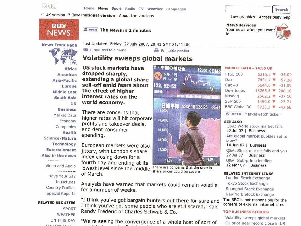
27 July Guardian.

“Down nearly 60 points at one stage, the FTSE recovered and put on the same amount again. But by the close it had slipped

back, down 36.0 points.”

“inject billions into the banking system”

Volatility

When is something volatile?

When values shifting/changing a lot

Vague concept

Can be formalized in various ways

There are empirical formulas as well as models

Merrill Lynch.

“Volatility.

A measure of the fluctuation in the market price of the underlying security.

Mathematically, volatility is the annualized standard deviation of returns.

A - Low; B - Medium; and C - High.”

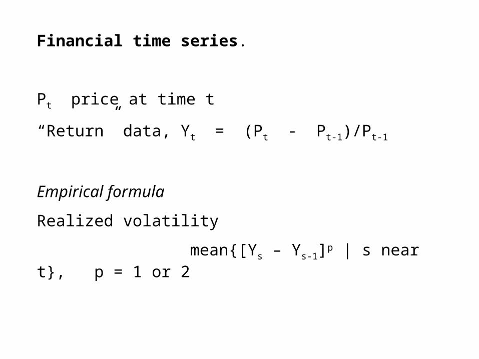
Financial time series.

Pt price at time t

“Return” data, Yt = (Pt - Pt-1)/Pt-1

Empirical formula

Realized volatility

mean{[Ys – Ys-1]p | s near t}, p = 1 or 2

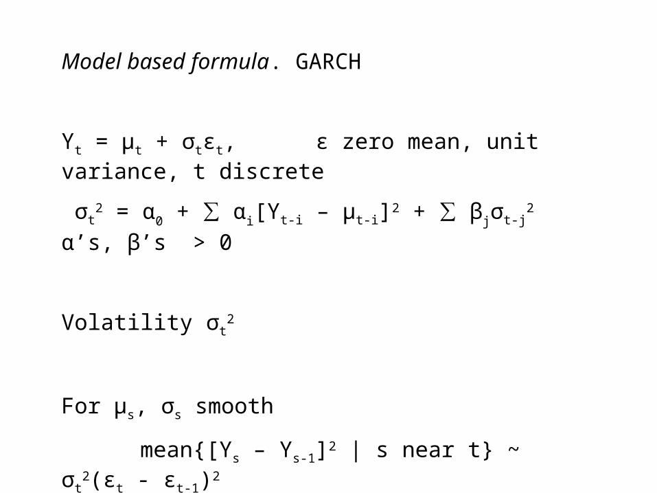
Model based formula. GARCH

Yt = μt + σtεt, ε zero mean, unit variance, t discrete

σt2 = α0 + ∑ αi[Yt-i – μt-i]2 + ∑ βjσt-j

2 α’s, β’s > 0

Volatility σt2

For μs, σs smooth

mean{[Ys – Ys-1]2 | s near t} ~ σt2(εt - εt-1)2

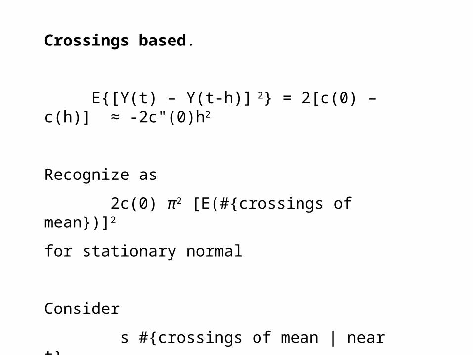
Crossings based.

E{[Y(t) – Y(t-h)] 2} = 2[c(0) – c(h)] ≈ -2c"(0)h2

Recognize as

2c(0) π2 [E(#{crossings of mean})]2

for stationary normal

Consider

s #{crossings of mean | near t}

as volatility measure

Example. Standard & Poors 500.

Weighted average of prices of 500 large companies in US stock market

Events

Great Crash Nov 1929

Asian Flu (Black Monday) Oct 1997

Other “crashes”: 1932, 1937, 1940, 1962, 1974, 1987

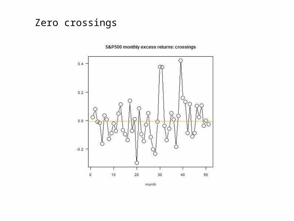
Zero crossings

S&P 500: realized volatility, model based, crossing based

Tsay (2002)

n= 792

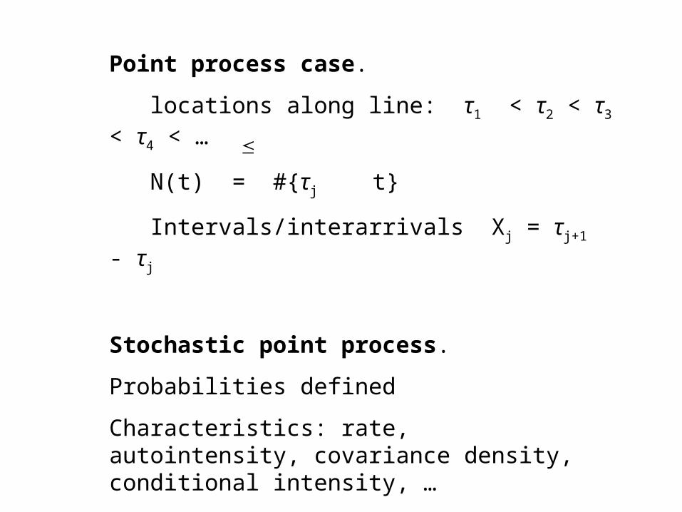
Point process case.

locations along line: τ1 < τ2 < τ3 < τ4 < …

N(t) = #{τj t}

Intervals/interarrivals Xj = τj+1 - τj

Stochastic point process.

Probabilities defined

Characteristics: rate, autointensity, covariance density, conditional intensity, …

E.g. Poisson, doubly stochastic Poisson

0-1 valued time series.

Zt = 0 or 1

Realized volatility

ave{ [Zs – Zs-1]2 | s near t }

Connection to zero crossings.

Zt= sgn(Yt), {Yt} ordinary t.s.

Σ [Zs – Zs-1]2 = #{zero crossings}

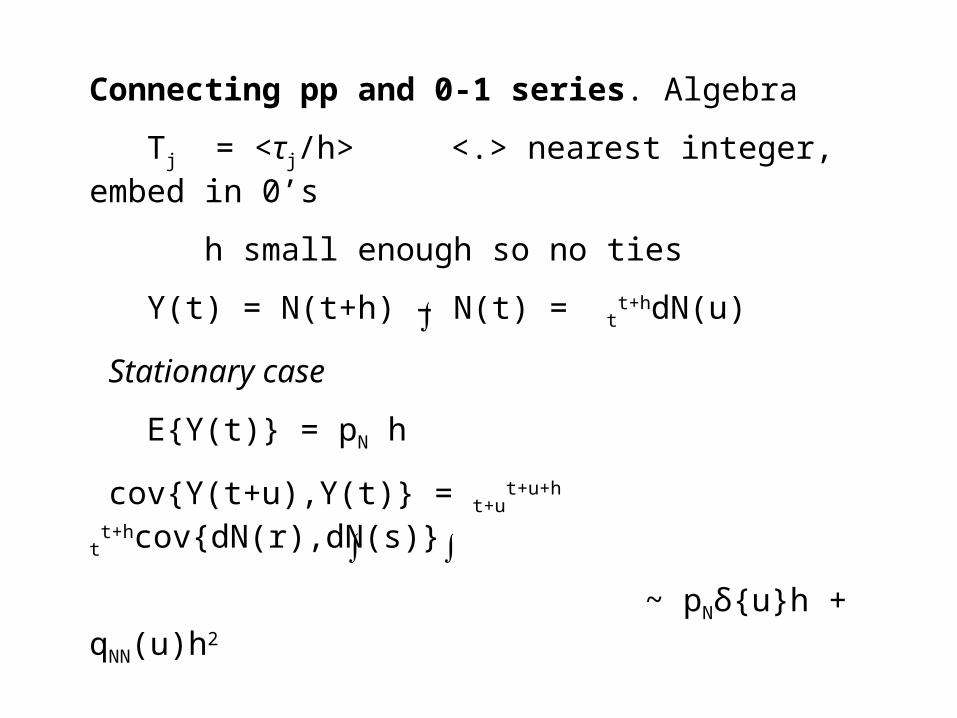
Connecting pp and 0-1 series. Algebra

Tj = <τj/h> <.> nearest integer, embed in 0’s

h small enough so no ties

Y(t) = N(t+h) – N(t) = tt+hdN(u)

Stationary case

E{Y(t)} = pN h

cov{Y(t+u),Y(t)} = t+ut+u+h t

t+hcov{dN(r),dN(s)}

~ pNδ{u}h + qNN(u)h2

as cov{dN(r),dN(s)} = [pN δ(r-s) + qNN(r-s)]dr ds,

rate, pN, covariance density, qNN(∙), Dirac delta, δ(∙)

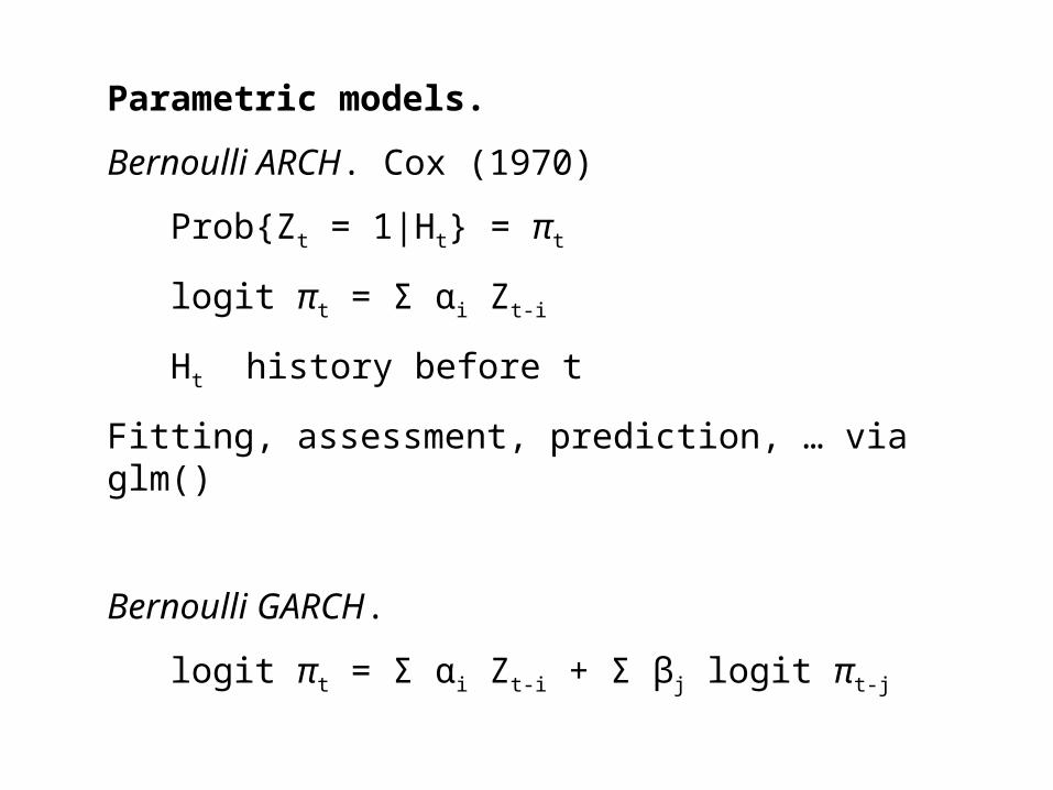
Parametric models.

Bernoulli ARCH. Cox (1970)

Prob{Zt = 1|Ht} = πt

logit πt = Σ αi Zt-i

Ht history before t

Fitting, assessment, prediction, … via glm()

Bernoulli GARCH.

logit πt = Σ αi Zt-i + Σ βj logit πt-j

Volatility πt or πt(1 - πt)?

Convento do Carmo

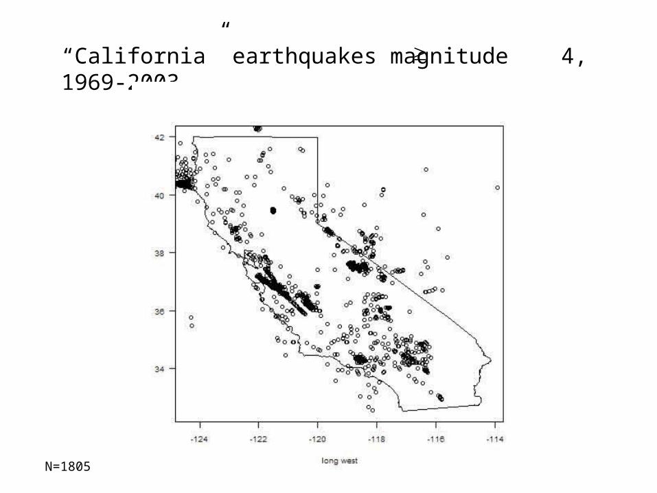
“California” earthquakes magnitude 4, 1969-2003

N=1805

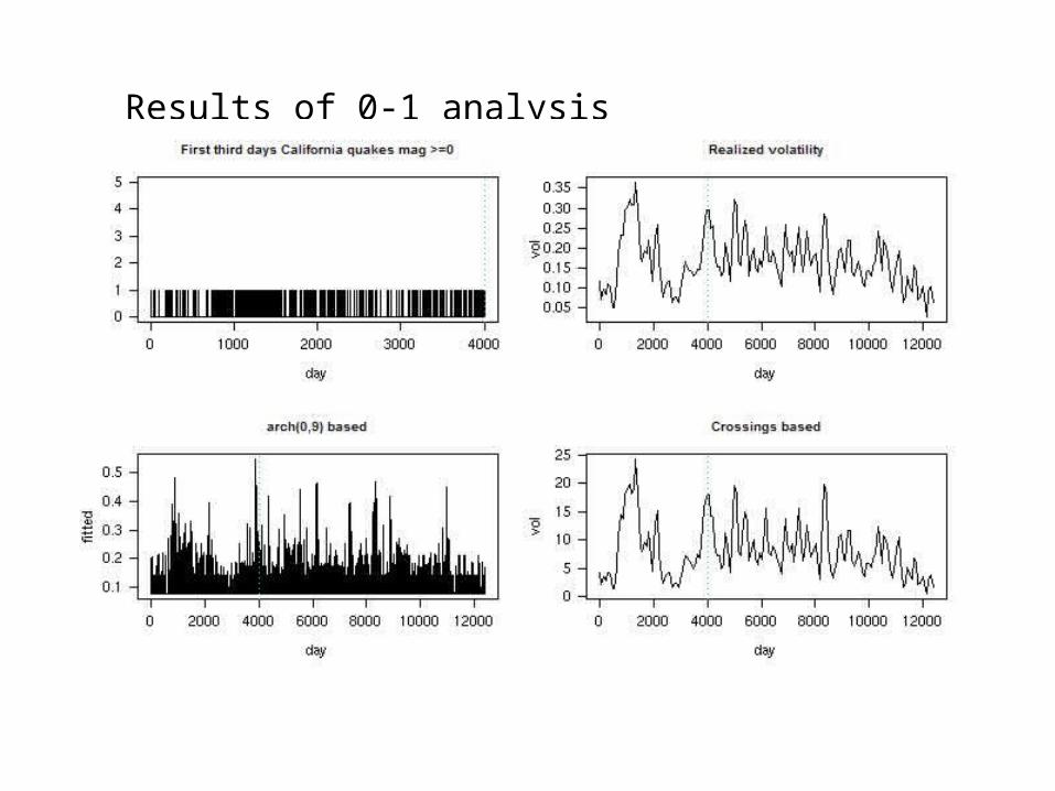
Results of 0-1 analysis

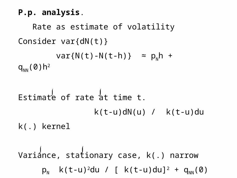
P.p. analysis.

Rate as estimate of volatility

Consider var{dN(t)}

var{N(t)-N(t-h)} ≈ pNh + qNN(0)h2

Estimate of rate at time t.

k(t-u)dN(u) / k(t-u)du

k(.) kernel

Variance, stationary case, k(.) narrow

pN k(t-u)2du / [ k(t-u)du]2 + qNN(0)

Example. Euro-USA exchange rate

Interval analysis.

Xj = τj – τj-1

Also stationary

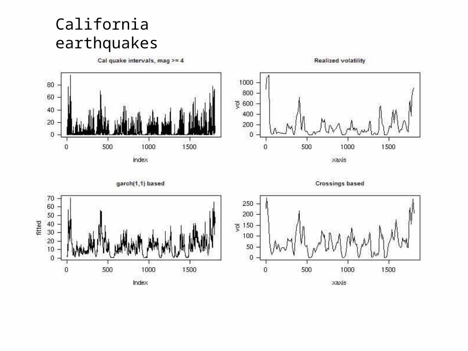
California earthquakes

Risk analysis. Time series case.

Assets Yt and probability p

VaR is the p-th quantile

Prob{Yt+1 – Yt VaR } = p

left tail

If approxmate distribution of Yt+1 – Yt by

Normal(0,σt)

volatility, σt, appears

Sometimes predictive model is built and fit to estimate VaR

Point process case.

Pulses arriving close together can damage

Number of oscillations to break object (Ang & Tang)

Suppose all points have the same value (mark), e.g. spike train.

Consider VaR of

Prob{N(t+u) – N(t) > VaR} = 1-p

Righthand tail

Examples.

S&P500: p=.05 method of moments quantile

VaR = $.0815

CA earthquakes: u = 7 days, p=.95 mom quantile

VaR = 28 events

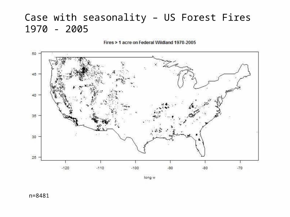
Case with seasonality – US Forest Fires 1970 - 2005

n=8481

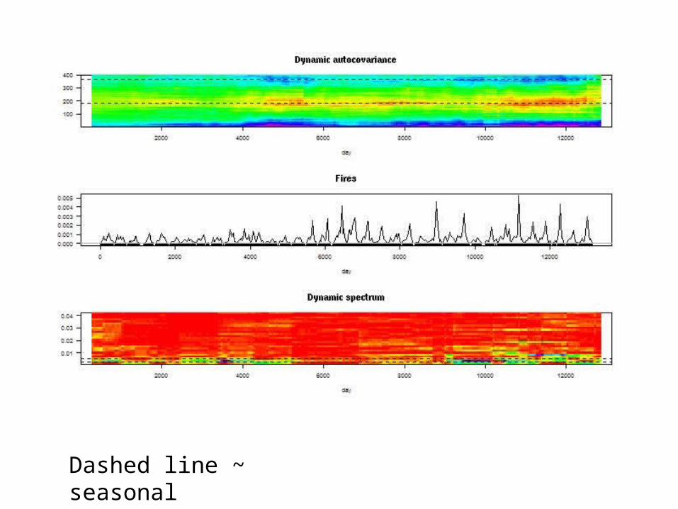
Dashed line ~ seasonal

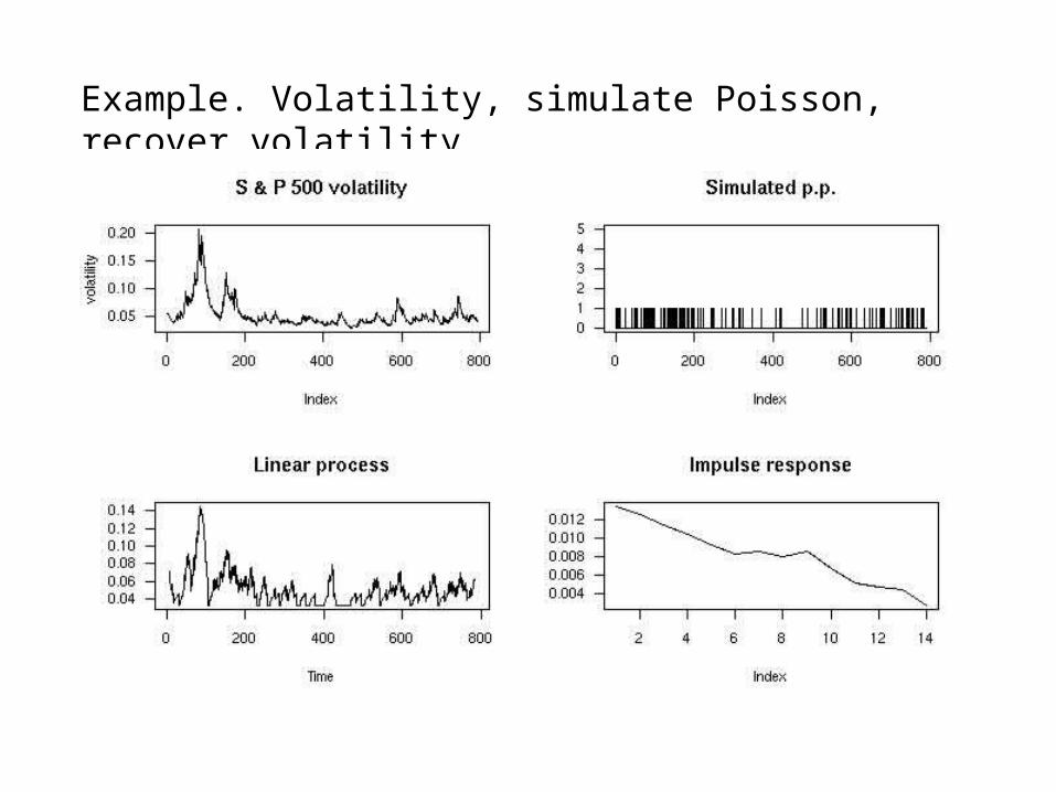
Example. Volatility, simulate Poisson, recover volatility

Conclusion.

Returning to the question, “Why bother with extension?

a) Perhaps will learn more about time series case

b) Pps are an interesting data type

c) Pps are building blocks

d) Volatility often considered risk measure for time series.”

The volatility can be the basic phenomenon

Another question.

“Is there a useful extension of the concept of volatility to point processes?”

The running rate

Gets at local behavior (prediction)

Some references.

Bouchard, J-P. and Potters, M. (2000). Theory of Financial Risk and Derivative Pricing. Cambridge

Dettling, M. and Buhlmann, P. “Volatility and risk estimation with linear and nonlinear methods based on high frequency data”

Tsay, R. S. (2002). Analysis of Financial Time Series. Wiley