Iterative Methods for Solving Large-scaleEigenvalue Problems

Chao Yang

Lawrence Berkeley National Laboratory, Berkeley, CA

November 19, 2015

Outline

I Krylov subspace methods

I Jacobi-Davidson

I Locally optimal conjugate gradient

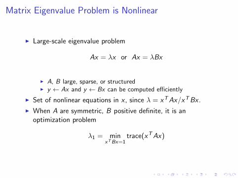
Matrix Eigenvalue Problem is Nonlinear

I Large-scale eigenvalue problem

Ax = λx or Ax = λBx

I A, B large, sparse, or structuredI y ← Ax and y ← Bx can be computed efficiently

I Set of nonlinear equations in x , since λ = xTAx/xTBx .

I When A are symmetric, B positive definite, it is anoptimization problem

λ1 = minxTBx=1

trace(xTAx)

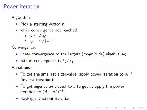
Power iteration

Algorithm:

I Pick a starting vector v0I while convergence not reached

I w ← Av0;I v0 ← w/‖w‖;

Convergence:

I linear convergence to the largest (magnitude) eigenvalue;

I rate of convergence is λ2/λ1;

Variations:

I To get the smallest eigenvalue, apply power iteration to A−1

(inverse iteration);

I To get eigenvalue closest to a target σ, apply the poweriteration to (A− σI )−1;

I Rayleigh-Quotient iteration

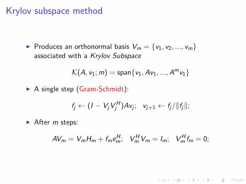
Krylov subspace method

I Produces an orthonormal basis Vm = {v1, v2, ..., vm}associated with a Krylov Subspace

K(A, v1;m) = span{v1,Av1, ...,Amv1}

I A single step (Gram-Schmidt):

fj ← (I − VjVHj )Avj ; vj+1 ← fj/‖fj‖;

I After m steps:

AVm = VmHm + fmeHm ; VH

mVm = Im; VHm fm = 0;

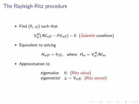
The Rayleigh-Ritz procedure

I Find (θi , yi ) such that

VHm (AVmy − θVmy) = 0 (Galerkin condition)

I Equivalent to solving

Hmyi = θiyi , where Hm = VHmAVm.

I Approximation to

eigenvalue θi (Ritz value)eigenvector zi = Vmyi (Ritz vector)

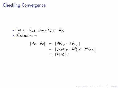
Checking Convergence

I Let z = Vmy , where Hmy = θy ;

I Residual norm

‖Az − θz‖ = ‖AVmy − θVmy‖= ‖(VmHm + feHm)y − θVmy‖= ‖f ‖|eHmy |

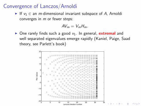
Convergence of Lanczos/ArnoldiI If v1 ∈ an m-dimensional invariant subspace of A, Arnoldi

converges in m or fewer steps:

AVm = VmHm.

I One rarely finds such a good v1. In general, extremal andwell separated eigenvalues emerge rapidly (Kaniel, Paige, Saadtheory, see Parlett’s book)

0 5 10 15 20 25 30 35−20

−15

−10

−5

0

5

10

15

20

Lanczos iteration number

Ritz v

alu

es

Computation Cost and Acceleration Methods

Cost:

I Storage for Vm, Hm: O(nm + m2);

I Orthogonalization fm ← (I − VmVHm )Avm: O(nm2);

I Eigen-analysis of Hm: O(m3);

I MATVEC y ← Ax : varies with applications;

Acceleration:

I Method of implicit restart

{polynomialrational

I Method of spectral transformation

{polynomialrational

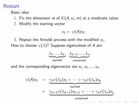
RestartBasic idea:

1. Fix the dimension m of K(A, v1;m) at a moderate value;

2. Modify the starting vector

v1 ← ψ(A)v1;

3. Repeat the Arnoldi process with the modified v1;

How to choose ψ(λ)? Suppose eigenvalues of A are:

λ1, ..., λk ,︸ ︷︷ ︸wanted

λk+1, ..., λn︸ ︷︷ ︸unwanted

,

and the corresponding eigenvector are x1, x2, ..., xn.

ψ(A)v1 = γ1ψ(λ1)x1 + · · ·+ γkψ(λk)xk︸ ︷︷ ︸wanted

+ γk+1ψ(λk+1)xk+1 + · · ·+ γnψ(λn)xn︸ ︷︷ ︸unwanted

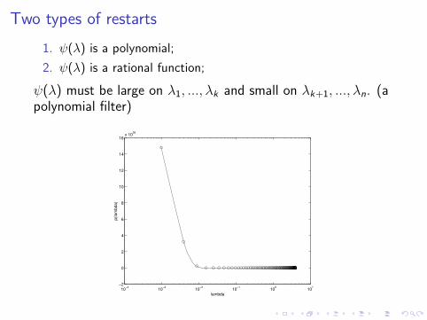
Two types of restarts

1. ψ(λ) is a polynomial;

2. ψ(λ) is a rational function;

ψ(λ) must be large on λ1, ..., λk and small on λk+1, ..., λn. (apolynomial filter)

10−4

10−3

10−2

10−1

100

101

−2

0

2

4

6

8

10

12

14

16x 10

30

lambda

p(la

mb

da

)

Implicit Restart

1. Do not form v1 ← ψ(A)v1 explicitly;

2. Do not repeat the Arnoldi iteration from the first column;

Need to understand the connection between Arnoldi and QR(RQ)· · ·

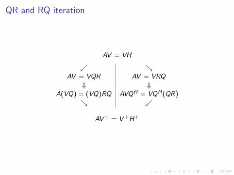
QR and RQ iteration

AV = VH

↙ ↘AV = VQR AV = VRQ

⇓ ⇓A(VQ) = (VQ)RQ AVQH = VQH(QR)

↘ ↙

AV+ = V+H+

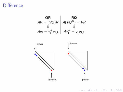
Difference

QR RQAV = (VQ)R A(VQH) = VR

⇓ ⇓Av1 = v+1 ρ1,1 Av+1 = v1ρ1,1

power inverse

powerinverse

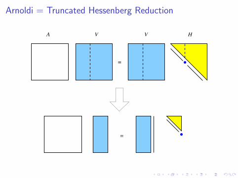
Arnoldi = Truncated Hessenberg Reduction

=

=

VA V H

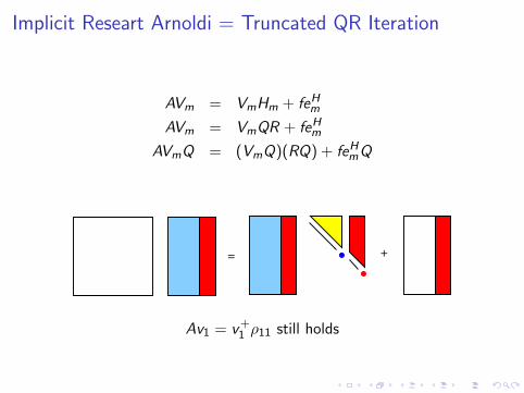
Implicit Researt Arnoldi = Truncated QR Iteration

AVm = VmHm + feHm

AVm = VmQR + feHm

AVmQ = (VmQ)(RQ) + feHmQ

= +

Av1 = v+1 ρ11 still holds

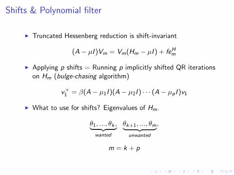
Shifts & Polynomial filter

I Truncated Hessenberg reduction is shift-invariant

(A− µI )Vm = Vm(Hm − µI ) + feHm

I Applying p shifts = Running p implicitly shifted QR iterationson Hm (bulge-chasing algorithm)

v+1 = β(A− µ1I )(A− µ2I ) · · · (A− µpI )v1

I What to use for shifts? Eigenvalues of Hm.

θ1, ..., θk ,︸ ︷︷ ︸wanted

θk+1, ..., θm︸ ︷︷ ︸unwanted

,

m = k + p

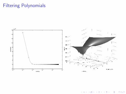
Filtering Polynomials

10−4

10−3

10−2

10−1

100

101

−2

0

2

4

6

8

10

12

14

16x 10

30

lambda

p(la

mb

da

)

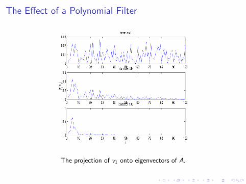
The Effect of a Polynomial Filter

The projection of v1 onto eigenvectors of A.

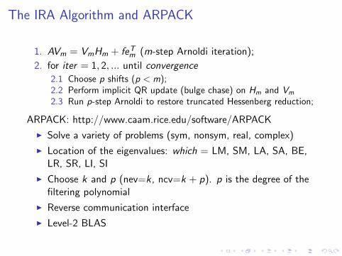
The IRA Algorithm and ARPACK

1. AVm = VmHm + feTm (m-step Arnoldi iteration);

2. for iter = 1, 2, ... until convergence

2.1 Choose p shifts (p < m);2.2 Perform implicit QR update (bulge chase) on Hm and Vm

2.3 Run p-step Arnoldi to restore truncated Hessenberg reduction;

ARPACK: http://www.caam.rice.edu/software/ARPACK

I Solve a variety of problems (sym, nonsym, real, complex)

I Location of the eigenvalues: which = LM, SM, LA, SA, BE,LR, SR, LI, SI

I Choose k and p (nev=k, ncv=k + p). p is the degree of thefiltering polynomial

I Reverse communication interface

I Level-2 BLAS

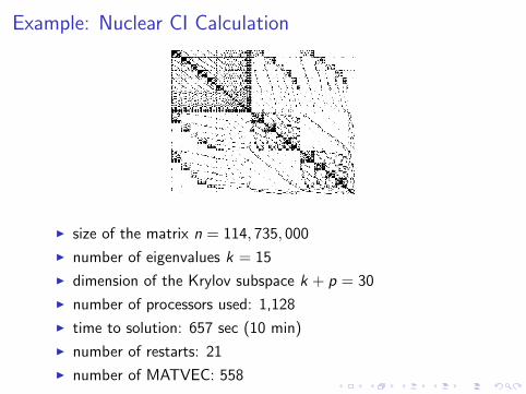
Example: Nuclear CI Calculation

I size of the matrix n = 114, 735, 000

I number of eigenvalues k = 15

I dimension of the Krylov subspace k + p = 30

I number of processors used: 1,128

I time to solution: 657 sec (10 min)

I number of restarts: 21

I number of MATVEC: 558

The Limitation of a Krylov Subspace

I May require a high degree polynomial φ(λ) to produce anaccurate approximation z = φ(A)v0;

I Subspace of large dimensionI Many restarts

I Spectral transformation may be prohibitively costly (sometimeimpossible)

I Not easy to introduce a preconditioner

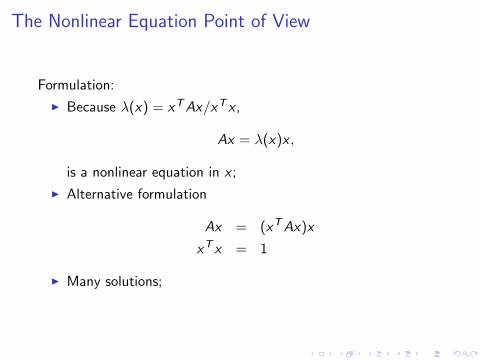
The Nonlinear Equation Point of View

Formulation:

I Because λ(x) = xTAx/xT x ,

Ax = λ(x)x ,

is a nonlinear equation in x ;

I Alternative formulation

Ax = (xTAx)x

xT x = 1

I Many solutions;

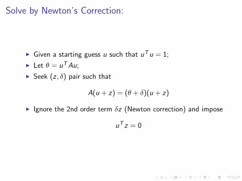
Solve by Newton’s Correction:

I Given a starting guess u such that uTu = 1;

I Let θ = uTAu;

I Seek (z , δ) pair such that

A(u + z) = (θ + δ)(u + z)

I Ignore the 2nd order term δz (Newton correction) and impose

uT z = 0

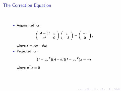
The Correction Equation

I Augmented form(A− θI uuT 0

)(z−δ

)=

(−r0

),

where r = Au − θu;

I Projected form

(I − uuT )(A− θI )(I − uuT )z = −r

where uT z = 0

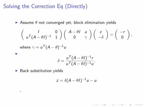
Solving the Correction Eq (Directly)

I Assume θ not converged yet, block elimination yields(I 0

uT (A− θI )−1 1

)(A− θI u

0 γ

)(z−δ

)=

(−r0

),

where γ = uT (A− θ)−1u

I

δ =uT (A− θI )−1r

uT (A− θI )−1u.

I Back substitution yields

z = δ(A− θI )−1u − u

,

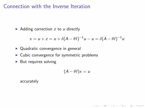
Connection with the Inverse Iteration

I Adding correction z to u directly

x = u + z = u + δ(A− θI )−1u − u = δ(A− θI )−1u

I Quadratic convergence in general

I Cubic convergence for symmetric problems

I But requires solving

(A− θI )x = u

accurately

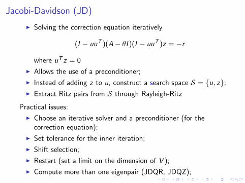
Jacobi-Davidson (JD)

I Solving the correction equation iteratively

(I − uuT )(A− θI )(I − uuT )z = −r

where uT z = 0

I Allows the use of a preconditioner;

I Instead of adding z to u, construct a search space S = {u, z};I Extract Ritz pairs from S through Rayleigh-Ritz

Practical issues:

I Choose an iterative solver and a preconditioner (for thecorrection equation);

I Set tolerance for the inner iteration;

I Shift selection;

I Restart (set a limit on the dimension of V );

I Compute more than one eigenpair (JDQR, JDQZ);

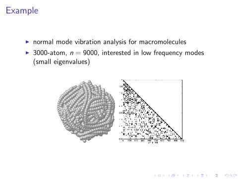
Example

I normal mode vibration analysis for macromolecules

I 3000-atom, n = 9000, interested in low frequency modes(small eigenvalues)

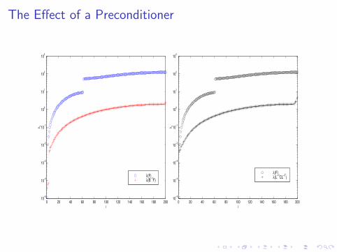
The Effect of a Preconditioner

0 20 40 60 80 100 120 140 160 180 20010

−5

10−4

10−3

10−2

10−1

100

101

102

103

i

λi

λ(F)λ(B

−1F)

0 20 40 60 80 100 120 140 160 180 20010

−5

10−4

10−3

10−2

10−1

100

101

102

103

i

λi

λ(F)λ(L

−1CL

−T)

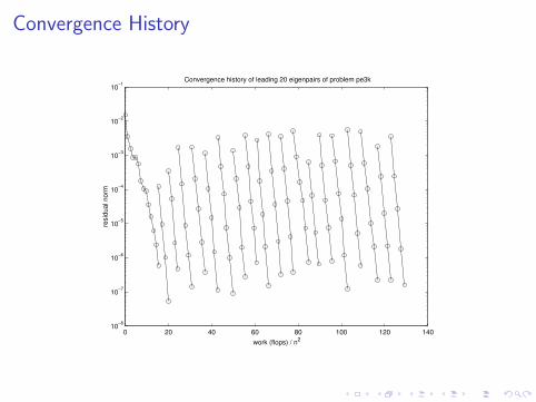
Convergence History

0 20 40 60 80 100 120 14010

−8

10−7

10−6

10−5

10−4

10−3

10−2

10−1

Convergence history of leading 20 eigenpairs of problem pe3k

work (flops) / n2

resid

ua

l n

orm

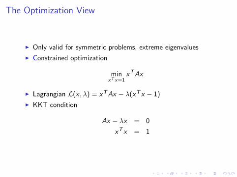
The Optimization View

I Only valid for symmetric problems, extreme eigenvalues

I Constrained optimization

minxT x=1

xTAx

I Lagrangian L(x , λ) = xTAx − λ(xT x − 1)

I KKT condition

Ax − λx = 0

xT x = 1

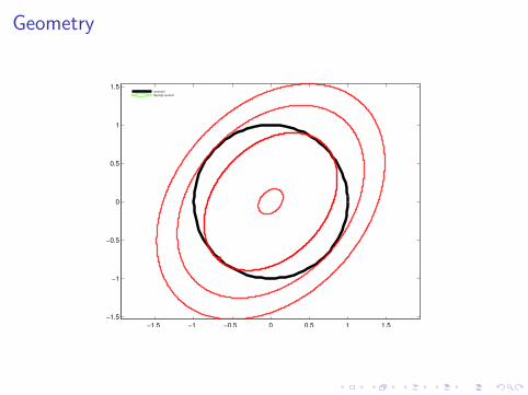
Geometry

−1.5 −1 −0.5 0 0.5 1 1.5

−1.5

−1

−0.5

0

0.5

1

1.5constraint

Rayleigh quotient

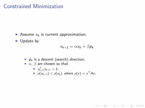
Constrained Minimization

I Assume xk is current approximation;

I Update byxk+1 = αxk + βpk

I pk is a descent (search) direction;I α, β are chosen so that

I xTk+1xk+1 = 1;

I ρ(xk+1) < ρ(xk), where ρ(x) = xTAx ;

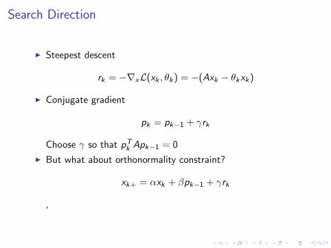
Search Direction

I Steepest descent

rk = −∇xL(xk , θk) = −(Axk − θkxk)

I Conjugate gradient

pk = pk−1 + γrk

Choose γ so that pTk Apk−1 = 0

I But what about orthonormality constraint?

xk+ = αxk + βpk−1 + γrk

,

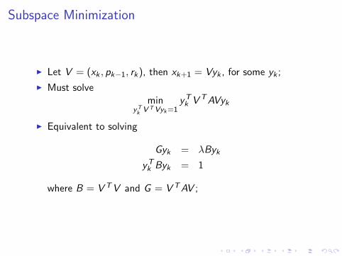
Subspace Minimization

I Let V = (xk , pk−1, rk), then xk+1 = Vyk , for some yk ;

I Must solvemin

yTk VTVyk=1

yTk V TAVyk

I Equivalent to solving

Gyk = λByk

yTk Byk = 1

where B = V TV and G = V TAV ;

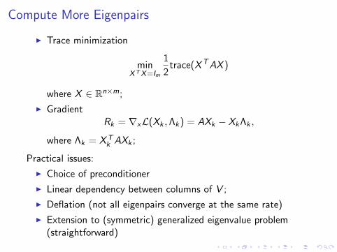
Compute More Eigenpairs

I Trace minimization

minXTX=Im

1

2trace(XTAX )

where X ∈ Rn×m;

I GradientRk = ∇xL(Xk ,Λk) = AXk − XkΛk ,

where Λk = XTk AXk ;

Practical issues:

I Choice of preconditioner

I Linear dependency between columns of V ;

I Deflation (not all eigenpairs converge at the same rate)

I Extension to (symmetric) generalized eigenvalue problem(straightforward)

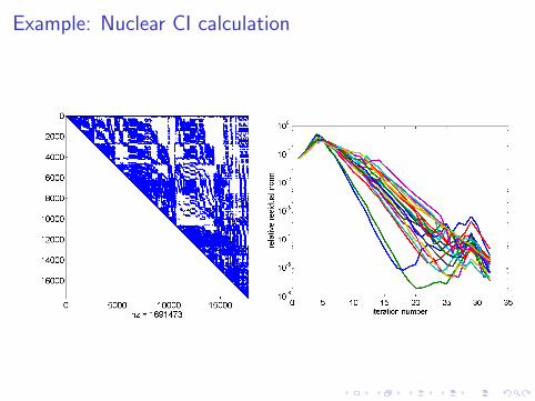
Example: Nuclear CI calculation

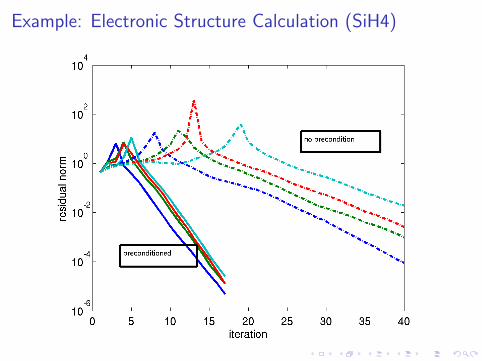
Example: Electronic Structure Calculation (SiH4)

Conclusion

I It all starts from power iteration

I Krylov subspace methods

I Implcitly restarted Arnoldi and its connection with QR

I Jacobi-Davidson

I Optimization based approach