Experimental Study of the HUM Control Operator for Linear ... · This allows us to obtain...
72
Experimental Study of the HUM Control Operator for Linear Waves Gilles Lebeau *† Universit´ e de Nice Ma¨ elle Nodet ‡ Universit´ e de Grenoble, INRIA November 1, 2018 Abstract We consider the problem of the numerical approximation of the lin- ear controllability of waves. All our experiments are done in a bounded domain Ω of the plane, with Dirichlet boundary conditions and internal control. We use a Galerkin approximation of the optimal control operator of the continuous model, based on the spectral theory of the Laplace op- erator in Ω. This allows us to obtain surprisingly good illustrations of the main theoretical results available on the controllability of waves, and to formulate some questions for the future analysis of optimal control theory of waves. * Laboratoire J.-A. Dieudonn´ e, Parc Valrose, Nice, France, [email protected] † Institut Universitaire de France ‡ Laboratoire J. Kuntzmann, Domaine Universitaire, Grenoble, France, [email protected] 1 arXiv:0904.3509v1 [math.OC] 22 Apr 2009
Transcript of Experimental Study of the HUM Control Operator for Linear ... · This allows us to obtain...
Experimental Study of the HUM Control
Operator for Linear Waves
Gilles Lebeau∗†
Universite de NiceMaelle Nodet‡
Universite de Grenoble, INRIA
November 1, 2018
Abstract
We consider the problem of the numerical approximation of the lin-ear controllability of waves. All our experiments are done in a boundeddomain Ω of the plane, with Dirichlet boundary conditions and internalcontrol. We use a Galerkin approximation of the optimal control operatorof the continuous model, based on the spectral theory of the Laplace op-erator in Ω. This allows us to obtain surprisingly good illustrations of themain theoretical results available on the controllability of waves, and toformulate some questions for the future analysis of optimal control theoryof waves.
∗Laboratoire J.-A. Dieudonne, Parc Valrose, Nice, France, [email protected]†Institut Universitaire de France‡Laboratoire J. Kuntzmann, Domaine Universitaire, Grenoble, France,
1
arX
iv:0
904.
3509
v1 [
mat
h.O
C]
22
Apr
200
9
Contents
1 Introduction 3
2 The analysis of the optimal control operator 52.1 The optimal control operator . . . . . . . . . . . . . . . . . 52.2 Theoretical results . . . . . . . . . . . . . . . . . . . . . . . 82.3 The spectral Galerkin method . . . . . . . . . . . . . . . . . 122.4 Computation of the discrete control operator . . . . . . . . 16
3 Numerical setup and validation 183.1 Geometries and control domains . . . . . . . . . . . . . . . 183.2 Time and space smoothing . . . . . . . . . . . . . . . . . . 183.3 Validation of the eigenvalues computation . . . . . . . . . . 193.4 Reconstruction error. . . . . . . . . . . . . . . . . . . . . . 193.5 Validation for the square geometry . . . . . . . . . . . . . . 19
3.5.1 Finite differences versus exact eigenvalues . . . . . . 193.5.2 Impact of the number of eigenvalues . . . . . . . . . 21
4 Numerical experiments 214.1 Frequency localization . . . . . . . . . . . . . . . . . . . . . 214.2 Space localization . . . . . . . . . . . . . . . . . . . . . . . . 22
4.2.1 Dirac experiments . . . . . . . . . . . . . . . . . . . 224.2.2 Box experiments in the square . . . . . . . . . . . . 22
4.3 Reconstruction error . . . . . . . . . . . . . . . . . . . . . . 234.4 Energy of the control function . . . . . . . . . . . . . . . . . 234.5 Condition number . . . . . . . . . . . . . . . . . . . . . . . 244.6 Non-controlling domains . . . . . . . . . . . . . . . . . . . . 25
Acknowledgement 25
References 26
List of Figures 28
List of Tables 67
2
1 Introduction
This paper is devoted to the experimental study of the exact controlla-bility of waves. All our experiments will be done in a bounded domain Ωof the plane, with Dirichlet boundary conditions and with internal con-trol. We use the most natural approach for the numerical computation: aGalerkin approximation of the optimal control operator of the continuousmodel based on the spectral theory of the Laplace operator in Ω. This willallow us to obtain surprisingly good illustrations of the main theoreticalresults available on the controllability of waves, and to formulate somequestions for the future analysis of the optimal control theory of waves.
The problem of controllability for linear evolution equations and sys-tems has a long story for which we refer to the review of D.-L. Russel in[Rus78] and to the book of J. L. Lions [Lio88]. Concerning controllabil-ity of linear waves, the main theoretical result is the so called “Geomet-ric Control Condition” of C. Bardos, G. Lebeau and J. Rauch [BLR92],GCC in short, which gives a (almost) necessary and sufficient conditionfor exact controllability. This is a “geometrical optics” condition on thebehavior of optical rays inside Ω. Here, optical rays are just straight linesinside Ω, reflected at the boundary according to the Snell-Descartes lawof reflection. The precise definition of optical rays near points of tangencywith the boundary is given in the works of R. Melrose and J. Sjostrand[MS78] and [MS82]. For internal control, GCC asserts that waves in aregular bounded domain Ω are exactly controllable by control functionssupported in the closure of an open sub-domain U and acting during atime T , if (and only if, if one allows arbitrary small perturbations of thetime control T and of the control domain U)
GCC: every optical ray of length T in Ω enters the sub-domain U .
Even when GCC is satisfied, the numerical computation of the con-trol is not an easy task. The original approach consists first in discretizingthe continuous model, and then in computing the control of the discretesystem to use it as a numerical approximation of the continuous one.This method has been developed by R. Glowinski et al. (see [GLL90] and[GHL08]), and used for numerical experiments in [AL98]. However, asobserved in the first works of R. Glowinski, interaction of waves with anumerical mesh produces spurious high frequency oscillations. In fact, thediscrete model is not uniformly exactly controllable when the mesh sizegoes to zero, since the group velocity converges to zero when the solutionswavelength is comparable to the mesh size. In other words, the processesof numerical discretization and observation or control do not commute. Aprecise analysis of this lack of commutation and its impact on the com-putation of the control has been done by E. Zuazua in [Zua02] and [Zua05].
In this paper, we shall use another approach, namely we will dis-cretize the optimal control of the continuous model using a projectionof the wave equation onto the finite dimensional space spanned by theeigenfunctions ej of the Laplace operator in Ω with Dirichlet boundary
3
conditions, −4ej = ω2j ej , ej |∂Ω=0 , with ωj ≤ ω. Here, ω will be a cutoff
frequency at our disposal. We prove (see lemma 2 in section 2.3) thatwhen GCC is satisfied, our numerical control converges when ω → ∞to the optimal control of the continuous model . Moreover, when GCCis not satisfied, we will do experiments and we will see an exponentialblow-up in the cutoff frequency ω of the norm of the discretized optimalcontrol. These blow-up rates will be compared to theoretical results insection 2.3.
The paper is organized as follows.
Section 2 is devoted to the analysis of the optimal control operator forwaves in a bounded regular domain of Rd. In section 2.1, we recall thedefinition of the optimal control operator Λ. In section 2.2, we recall someknown theoretical results on Λ: existence, regularity properties and thefact that it preserves the frequency localization. We also state our firstconjecture, namely that the optimal control operator Λ is a microlocaloperator. In section 2.3, we introduce the spectral Galerkin approxima-tion M−1
T,ω of Λ, where ω is a cutoff frequency. We prove the convergence
of M−1T,ω toward Λ when ω → ∞, and we analyze the rate of this conver-
gence. We also state our second conjecture on the blow-up rate of M−1T,ω
when GCC is not satisfied. Finally, in section 2.4, we introduce the basisof the energy space in which we compute the matrix of the operator MT,ω.
Section 3 is devoted to the experimental validation of our Galerkinapproximation. In section 3.1 we introduce the 3 different domains of theplane for our experiments: square, disc and trapezoid. In the first twocases, the geodesic flow is totally integrable and the exact eigenfunctionsand eigenvalues of the Laplace operator with Dirichlet boundary condi-tion are known. This is not the case for the trapezoid. In section 3.2 weintroduce the two different choices of the control operator we use in our ex-periments. In the first case (non smooth case), we use χ(t, x) = 1[0,T ]1U .In the second case (smooth case), we use a suitable regularization of thefirst case (see formulas (66) and (67)). Perhaps the main contribution ofthis paper is to give an experimental evidence that the choice of a smoothenough control operator is the right way to get accuracy on control com-puting. In section 3.3, in the two cases of the square and the disc, wecompare the exact eigenvalues with the eigenvalues computed using the5-points finite difference approximation of the Laplace operator. In sec-tion 3.4, formula (69), we define the reconstruction error of our method.Finally, in section 3.5, in the case of the square geometry, we compare thecontrol function (we choose to reconstruct a single eigenvalue) when theeigenvalues and eigenvectors are computed either with finite differences orwith exact formulas, and we study the experimental convergence of ournumerical optimal control to the exact optimal control of the continuousmodel when the cutoff frequency goes to infinity.
The last section, 4, presents various numerical experiments which il-lustrate the theoretical results of section 2, and are in support of our two
4
conjectures. In section 4.1, our experiments illuminate the fact that theoptimal control operator preserves the frequency localization, and thatthis property is far much stronger when the control function is smooth,as predicted by theoretical results. In section 4.2, we use Dirac and boxexperiments to illustrate the fact that the optimal control operator showsa behavior very close to the behavior of a pseudo-differential operator:this is in support of our first conjecture. In section 4.3, we plot the re-construction error as a function of the cutoff frequency: this illuminateshow the rate of convergence of the Galerkin approximation depends onthe regularity of the control function. In section 4.4, we present variousresults on the energy of the control function. In section 4.5, we computethe condition number of the matrix MT,ω for a given control domain U , asa function of the control time T and the cutoff frequency ω. In particular,figures 31 and 32 are in support of our second conjecture on the blow-uprate of M−1
T,ω when GCC is not satisfied. In section 4.6, we perform ex-periments in the disc when GCC is not satisfied, for two different data:in the first case, every optical rays of length T starting at a point wherethe data is not small enters the control domain U , and we observe a rathergood reconstruction error if the cutoff frequency is not too high. In thesecond case, there exists an optical ray starting at a point where the datais not small and which never enters the control domain, and we observea very poor reconstruction at any cutoff frequency. This is a fascinatingphenomena which has not been previously studied in theoretical works. Itwill be of major practical interest to get quantitative results on the bestcutoff frequency which optimizes the reconstruction error (this optimalcutoff frequency is equal to ∞ when GCC is satisfied, the reconstructionerror being equal to 0 in that case), and to estimate the reconstruction er-ror at the optimal cutoff frequency. Clearly, our experiments indicate thata weak Geometric Control Condition associated to the data one wants toreconstruct will enter in such a study.
2 The analysis of the optimal control op-erator
2.1 The optimal control operator
Here we recall the basic facts we will need in our study of the optimalcontrol operator for linear waves. For more details on the HUM method,we refer to the book of J.-L. Lions [Lio88].
In the framework of the wave equation in a bounded open subset Ω ofRd with boundary Dirichlet condition, and for internal control the problemof controllability is stated in the following way. Let T be a positive time,U a non void open subset of Ω, and χ(t, x) as follows:
χ(t, x) = ψ(t)χ0(x) (1)
where χ0 is a real L∞ function on Ω, such that support(χ0) = U andχ0(x) is continuous and positive for x ∈ U , ψ ∈ C∞([0, T ]) and ψ(t) > 0
5
on ]0, T [. For a given f = (u0, u1) ∈ H10 (Ω)×L2(Ω), the problem is to find
a source v(t, x) ∈ L2(0, T ;L2(Ω)) such that the solution of the system8<:u = χv in ]0,+∞[×Ω
u|∂Ω = 0, t > 0(u|t=0, ∂tu|t=0) = (0, 0)
(2)
reaches the state f = (u0, u1) at time T . We first rewrite the wave oper-ator in (2) as a first order system. Let A be the matrix
iA =
„0 Id4 0
«(3)
Then A is a unbounded self-adjoint operator on H = H10 (Ω) × L2(Ω),
where the scalar product on H10 (Ω) is
RΩ∇u∇vdx and D(A) = u =
(u0, u1) ∈ H, A(u) ∈ H, u0|∂Ω = 0. Let λ =√−4D where −4D
is the canonical isomorphism from H10 (Ω) onto H−1(Ω). Then λ is an
isomorphism from H10 (Ω) onto L2(Ω). The operator B(t) given by
B(t) =
„0 0
χ(t, .)λ 0
«(4)
is bounded on H, and one has
B∗(t) =
„0 λ−1χ(t, .)0 0
«(5)
The system (2) is then equivalent to
(∂t − iA)f = B(t)g, f(0) = 0 (6)
with f = (u, ∂tu), g = (λ−1v, 0). For any g(t) ∈ L1([0,∞[, H), theevolution equation
(∂t − iA)f = B(t)g, f(0) = 0 (7)
admits a unique solution f = S(g) ∈ C0([0,+∞[, H) given by the Duhamelformula
f(t) =
Z t
0
ei(t−s)AB(s)g(s)ds (8)
Let T > 0 be given. Let RT be the reachable set at time T
RT = f ∈ H, ∃g ∈ L2([0, T ], H), f = S(g)(T ) (9)
Then RT is a linear subspace of H, and is the set of states of the systemthat one can reach in time T , starting from rest, with the action of anL2 source g filtered by the control operator B. The control problem con-sists in giving an accurate description of RT , and exact controllability isequivalent to the equality RT = H. Let us recall some basic facts.
Let H = L2([0, T ], H). Let F be the closed subspace of H spanned bysolutions of the adjoint evolution equation
F = h ∈ H, (∂t − iA∗)h = 0, h(T ) = hT ∈ H (10)
6
Observe that, in our context, A∗ = A, and the function h in (10) isgiven by h(t) = e−i(T−t)AhT . Let B∗ be the adjoint of the operatorg 7→ S(g)(T ). Then B∗ is the bounded operator from H into H definedby
B∗(hT )(t) = B∗(t)e−i(T−t)AhT (11)
For any g ∈ L2([0, T ], H), one has, with fT = S(g)(T ) and h(s) =e−i(T−s)AhT the fundamental identity
(fT |hT )H =
Z T
0
(B(s)g(s)|h(s))ds = (g|B∗(hT ))H (12)
From (12), one gets easily that the following holds true
RT is a dense subspace of H ⇐⇒ B∗ is an injective operator (13)
which shows that approximate controllability is equivalent to a uniquenessresult on the adjoint equation. Moreover, one gets from (12), using theRiesz and closed graph theorems, that the following holds true
RT = H ⇐⇒ ∃C, ‖h‖ ≤ C‖B∗h‖ ∀h ∈ H (14)
This is an observability inequality, and B∗ is called the observability op-erator. We rewrite the observability inequality (14) in a more explicitform
∃C, ‖h‖2H ≤ CZ T
0
‖B∗(s)e−i(T−s)Ah‖2Hds ∀h ∈ H (15)
Assuming that (15) holds true, then RT = H, Im(B∗) is a closedsubspace of H, and B∗ is an isomorphism of H onto Im(B∗). For anyf ∈ H, let Cf be the set of control functions g driving 0 to f in time T
Cf =
g ∈ L2([0, T ], H), f =
Z T
0
ei(T−s)AB(s)g(s)ds
ff(16)
From (12), one gets
Cf = g0 + (ImB∗)⊥, g0 ∈ ImB∗ ∩ Cf (17)
and g0 = B∗hT is the optimal control in the sense that
min‖g‖L2([0,T ],H), g ∈ Cf is achieved at g = g0 (18)
Let Λ : H → H, Λ(f) = hT be the control map, so that the optimalcontrol g0 is equal to g0(t) = B∗(t)e−i(T−t)AΛ(f). Then Λ is exactly theinverse of the map MT : H → H with
MT =
Z T
0
m(T − t)dt =
Z T
0
m(s)ds
m(s) = eisAB(T − s)B∗(T − s)e−isA∗
(19)
Observe that m(s) = m∗(s) is a bounded, self-adjoint, non-negative oper-ator on H. Exact controllability is thus equivalent to
∃C > 0, MT =
Z T
0
ei(T−t)A„
0 00 χ2(t, .)
«e−i(T−t)Adt ≥ CId (20)
7
With Λ = M−1T , the optimal control is then given by g0(t) = B∗(t)e−i(T−t)AΛ(f)
and is by (5) of the form g0 = (λ−1χ∂tw, 0) where w(t) = e−i(T−t)AΛ(f)is the solution of
w = 0 in R× Ω, w|∂Ω = 0(w(T, .), ∂tw(T, .)) = Λ(f)
(21)
Thus, the optimal control function v in (2) is equal to v = χ∂tw, wherew is the solution of the dual problem (21). The operator Λ = M−1
T , withMT given by (20) is called the optimal control operator.
2.2 Theoretical results
In this section we recall some theoretical results on the analysis of theoptimal control operator Λ. We will assume here that Ω is a boundedopen subset of Rd with smooth boundary ∂Ω, and that any straight linein Rd has only finite order of contacts with the boundary. In that case,optical rays are uniquely defined. See an example of such rays in figure 1.
[Figure 1 about here.]
Let M = Ω× Rt. The phase space is
bT ∗M = T ∗M \ T ∗∂M ' T ∗M ∪ T ∗∂M.
The characteristic variety of the wave operator is the closed subset Σof bT ∗M of points (x, t, ξ, τ) such that |τ | = |ξ| when x ∈ Ω and |τ | ≥ |ξ|when x ∈ ∂Ω. Let bS∗Ω be the set of points
bS∗Ω = (x0, ξ0), with |ξ0| = 1 if x0 ∈ Ω, |ξ0| ≤ 1 if x0 ∈ ∂Ω
For ρ0 = (x0, ξ0) ∈ bS∗Ω, and τ = ±1, we shall denote by s →
(γρ0(s), t − sτ, τ), s ∈ R the generalized bicharacteristic ray of the waveoperator, issued from (x0, ξ0, t, τ). For the construction of the Melrose-Sjostrand flow, we refer to [MS78], [MS82] and to [Hor85], vol 3, chapterXXIV . Then s → γρ0(s) = (x(ρ0, s), ξ(ρ0, s)) is the optical ray startingat x0 in the direction ξ0. When x0 ∈ ∂Ω and |ξ0| < 1, then the right(respectively left) derivative of x(ρ0, s) at s = 0 is equal to the unit vectorin Rd which projects on ξ0 ∈ T ∗∂Ω and which points inside (respectivelyoutside) Ω. In all other cases, x(ρ0, s) is derivable at s = 0 with derivativeequal to ξ0.
We first recall the theorem of [BLR92], which gives the existence ofthe operator Λ:
Theorem 1 If the geometric control condition GCC holds true, then MT
is an isomorphism.
Next, we recall some new theoretical results obtained in [DL09]. Forthese results, the choice of the control function χ(t, x) in (1) will be es-sential.
Definition 1 The control function χ(t, x) = ψ(t)χ0(x) is smooth if χ0 ∈C∞(Ω) and ψ(t) is flat at t = 0 and t = T .
8
For s ∈ R, we denote byHs(Ω,4) the domain of the operator (−4Dirichlet)s/2.
One has H0(Ω,4) = L2(Ω), H1(Ω,4) = H10 (Ω), and if (ej)j≥1 is an L2
orthonormal basis of eigenfunctions of −4 with Dirichlet boundary con-ditions, −4ej = ω2
j ej , 0 < ω1 ≤ ω2 ≤ ..., one has
Hs(Ω,4) = f ∈ D′(Ω), f =Xj
fjej ,Xj
ω2sj |fj |2 <∞ (22)
The following result of [DL09] says that, under the hypothesis thatthe control function χ(t, x) is smooth, the optimal control operator Λpreserves the regularity:
Theorem 2 Assume that the geometric control condition GCC holdstrue, and that the control function χ(t, x) is smooth. Then the optimalcontrol operator Λ is an isomorphism of Hs+1(Ω,∆) ⊕ Hs(Ω,∆) for alls ≥ 0.
Observe that theorem 1 is a particular case of theorem 2 with s = 0.In our experimental study, we will see in section 4.3 that the regularityof the control function χ(t, x) is not only a nice hypothesis to get theo-retical results. It is also very efficient to get accuracy in the numericalcomputation of the control function. In other words, the usual choice ofthe control function χ(t, x) = 1[0,T ]1U is a very poor idea to compute acontrol.
The next result says that the optimal control operator Λ preserves thefrequency localization. To state this result we briefly introduce the mate-rial needed for the Littlewood-Paley decomposition. Let φ ∈ C∞([0,∞[),with φ(x) = 1 for |x| ≤ 1/2 and φ(x) = 0 for |x| ≥ 1. Set ψ(x) =φ(x)−φ(2x). Then ψ ∈ C∞0 (R∗), ψ vanishes outside [1/4, 1], and one has
φ(s) +
∞Xk=1
ψ(2−ks) = 1, ∀s ∈ [0,∞[
Set ψ0(s) = φ(s) and ψk(s) = ψ(2−ks) for k ≥ 1. We then define thespectral localization operators ψk(D), k ∈ N, in the following way: foru =
Pj ajej , we define
ψk(D)u =Xj
ψk(ωj)ajej (23)
One hasPk ψk(D) = Id and ψi(D)ψj(D) = 0 for |i− j| ≥ 2. In addition,
we introduce
Sk(D) =
kXj=0
ψj(D) = ψ0(2−kD), k ≥ 0 (24)
Obviously, the operators ψk(D) and Sk(D) acts as bounded operators onH = H1
0 ×L2. The spectral localization result of [DL09] reads as follows.
9
Theorem 3 Assume that the geometric control condition GCC holdstrue, and that the control function χ(t, x) is smooth. There exists C > 0such that for every k ∈ N, the following inequality holds true
‖ψk(D)Λ− Λψk(D)‖H ≤ C2−k
‖Sk(D)Λ− ΛSk(D)‖H ≤ C2−k(25)
Theorem 3 states that the optimal control operator Λ, up to lower or-der terms, acts individually on each frequency block of the solution. Forinstance, if en is the n-th eigenvector of the orthonormal basis of L2(Ω),if one drives the data (0, 0) to (en, 0) in (2) using the optimal control,both the solution u and control v in equation (2) will essentially live atfrequency ωn for n large. We shall do experiments on this fact in section4.1, and we will clearly see the impact of the regularity of the control func-tion χ(t, x) on the accuracy of the frequency localization of the numericalcontrol.
Since by the above results the optimal control operator Λ preservesthe regularity and the frequency localization, it is very natural to expectthat Λ is in fact a micro-local operator, and in particular preserves thewave front set. For an introduction to micro-local analysis and pseudo-differential calculus, we refer to [Tay81] and [Hor85]. In [DL09], it isproved that the optimal control operator Λ for waves on a compact Rie-mannian manifold without boundary is in fact an elliptic 2× 2 matrix ofpseudo-differential operators. This is quite an easy result, since if χ(t, x)is smooth the Egorov theorem implies that the operator MT given by(20) is a 2× 2 matrix of pseudo-differential operators. Moreover, the ge-ometric control condition GCC implies easily that MT is elliptic. SinceMT is self adjoint, the fact that MT is an isomorphism follows then fromKer(MT ) = 0, which is equivalent to the injectivity of B∗. This isproved in [BLR92] as a consequence of the uniqueness theorem of Calderonfor the elliptic second order operator 4. Then it follows that its inverseΛ = M−1
T is an elliptic pseudo-differential operator.
In our context, for waves in a bounded regular open subset Ω of Rdwith boundary Dirichlet condition, the situation is far much complicated,since there is no Egorov theorem in the geometric setting of a manifoldwith boundary. In fact, the Melrose-Sjostrand theorem [MS78], [MS82]on propagation of singularities at the boundary (see also [Hor85], vol 3,chapter XXIV for a proof) implies that the operator MT given by (20)is a microlocal operator, but this is not sufficient to imply that its in-verse Λ is micro-local. However let ρ0 = (x0, ξ0) ∈ T ∗Ω, |ξ0| = 1 be apoint in the cotangent space such that the two optical rays defined bythe Melrose-Sjostrand flow (see [MS78], [MS82]) s ∈ [0, T ] → γ±ρ0(s) =(x(±ρ0, s), ξ(±ρ0, s)), with ±ρ0 = (x0,±ξ0), starting at x0 in the direc-tions ±ξ0 have only transversal intersections with the boundary. Then itis not hard to show using formula (20) and the parametrix of the waveoperator, inside Ω and near transversal reflection points at the boundary∂Ω, as presented in figure 2, that MT is microlocally at ρ0 an elliptic 2×2matrix of elliptic pseudo-differential operators.
10
[Figure 2 about here.]
More precisely, let J be the isomorphism from H10 ⊕L2 on L2 ⊕L2 given
by
J =1
2
„λ −iλ i
«(26)
One has 2‖Ju‖2L2⊕L2 = ‖u‖2H10⊕L2 , and if u(t, x) is the solution of the
wave operator 2u = 0 with Dirichlet boundary conditions on ∂Ω, andCauchy data at time t0 equal to (u0, u1), then one has
λu(t, .) = λ cos((t− t0)λ)u0 + sin((t− t0)λ)u1
= ei(t−t0)λ“λu0−iu1
2
”+ e−i(t−t0)λ
“λu0+iu1
2
” (27)
so the effect of the isomorphism J is to split the solution u(t, x) into a sumof two waves with positive and negative temporal frequency. Moreover,one has
JeitAJ−1 =
„eitλ 0
0 e−itλ
«(28)
Then JMTJ−1 acts as a non negative self-adjoint operator on L2 ⊕ L2,
and is equal to
JMTJ−1 = 1
2
„Q+ −T−T ∗ Q−
«Q± =
R T0e±isλχ2(T − s, .)e∓isλds
T =R T
0eisλχ2(T − s, .)eisλds
(29)
From (29), using the parametrix of the wave operator, inside Ω and neartransversal reflection points at the boundary ∂Ω, and integration by partsto show that T is a smoothing operator, it is not difficult to get thatJMTJ
−1 is microlocally at ρ0 ∈ T ∗Ω a pseudo-differential operator oforder zero with principal symbol
σ0(JMTJ−1)(ρ0) = 1
2
„q+(x0, ξ0) 0
0 q−(x0, ξ0)
«q±(x0, ξ0) =
R T0χ2(T − s, x(±ρ0, s))ds
(30)
Obviously, condition (GCC) guarantees that σ0(JMTJ−1)(ρ0) is elliptic,
and therefore JΛJ−1 will be at ρ0 a pseudo-differential operator of orderzero with principal symbol
σ0(JΛJ−1)(ρ0) = 2
„q−1+ (x0, ξ0) 0
0 q−1− (x0, ξ0)
«(31)
Therefore, the only difficulty in order to prove that Λ is a microlocaloperator is to get a precise analysis of the structure of the operator MT
near rays which are tangent to the boundary. Since the set of ρ ∈b S∗Ω forwhich the optical ray γρ(s) has only transversal points of intersection withthe boundary is dense in T ∗Ω \T ∗∂Ω (see [Hor85]), it is not surprising thatour numerical experiments in section 4.2 (where we compute the optimalcontrol associated to a Dirac mass δx0 , x0 ∈ Ω), confirms the followingconjecture:
11
Conjecture 1 Assume that the geometric control condition GCC holdstrue, that the control function χ(t, x) is smooth, and that the optical rayshave no infinite order of contact with the boundary. Then Λ is a microlocaloperator.
Of course, part of the difficulty is to define correctly what is a mi-crolocal operator in our context. In the above conjecture, microlocal willimplies in particular that the optimal control operator Λ preserves thewave front set. A far less precise information is to know that Λ is a mi-crolocal operator at the level of microlocal defect measures, for which werefer to [Ger91]. But this is an easy by-product of the result of N. Burqand G. Lebeau in [BL01].
2.3 The spectral Galerkin method
In this section we describe our numerical approximation of the optimalcontrol operator Λ, and we give some theoretical results on the numericalapproximation MT,ω of the operator MT given by (20), even in the casewhere the geometric control condition GCC is not satisfied.
For any cutoff frequency ω, we denote by Πω the orthogonal projection,in the Hilbert space L2(Ω), on the finite dimensional linear subspace L2
ω
spanned by the eigenvectors ej for ωj ≤ ω. By the Weyl formula, if cddenotes the volume of the unit ball in Rd, one has
N(ω) = dim(L2ω) ' (2π)−dVol(Ω)cdω
d (ω → +∞) (32)
Obviously, Πω acts on H = H10 × L2 and commutes with eitA, λ and
J . We define the Galerkin approximation MT,ω of the operator MT asthe operator on L2
ω × L2ω
MT,ω = ΠωMTΠω =
Z T
0
ei(T−t)AΠω
„0 00 χ2(t, .)
«Πωe
−i(T−t)Adt (33)
Obviously, the matrix MT,ω is symmetric and non negative for the Hilbertstructure induced by H on L2
ω × L2ω, and by (19) one has with nω(t) =
B∗(t)Πωe−i(T−t)A
MT,ω =
Z T
0
n∗ω(t)nω(t)dt (34)
By (29) one has also
JMT,ωJ−1 = 1
2
„Q+,ω −Tω−T ∗ω Q−,ω
«Q±,ω =
R T0e±isλΠωχ
2(T − s, .)Πωe∓isλds
Tω =R T
0eisλΠωχ
2(T − s, .)Πωeisλds
(35)
Let us first recall two easy results. For convenience, we recall herethe proof of these results. The first result states that the matrix MT,ω isalways invertible.
Lemma 1 For any (non zero) control function χ(t, x), the matrix MT,ω
is invertible.
12
Proof. Let u = (u0, u1) ∈ L2ω × L2
ω such that MT,ω(u) = 0. By (34)one has
0 = (MT,ω(u)|u)H =
Z T
0
‖nω(t)(u)‖2Hdt.
This implies nω(t)(u) = 0 for almost all t ∈]0, T [. If u(t, x) is the solutionof the wave equation with Cauchy data (u0, u1) at time T , we thus getby (5) and (1) ψ(t)χ0(x)∂tu(t, x) = 0 for t ∈ [0, T ], and since ψ(t) > 0on ]0, T [ and χ0(x) > 0 on U , we get ∂tu(t, x) = 0 on ]0, T [×U . One hasu0 =
Pωj≤ω ajej(x), u1 =
Pωj≤ω bjej(x) and
∂tu(t, x) =Xωj≤ω
ωjaj sin((T − t)ωj)ej(x) +Xωj≤ω
bj cos((T − t)ωj)ej(x)
Thus we getPωj≤ω ωjajej(x) =
Pωj≤ω bjej(x) = 0 for x ∈ U , which
implies, since the eigenfunctions ej are analytic in Ω, that aj = bj = 0 forall j. 2
For any ω0 ≤ ω, we define Π⊥ω = 1−Πω, and we set
‖Π⊥ωΛΠω0‖H = rΛ(ω, ω0)
‖Π⊥ωMTΠω0‖H = rM (ω, ω0)(36)
Since the ranges of the operators ΛΠω0 and MTΠω0 are finite dimensionalvector spaces, one has for any ω0
limω→∞ rΛ(ω, ω0) = 0limω→∞ rM (ω, ω0) = 0
(37)
The second result states that when GCC holds true, the inverse matrixM−1T,ω converges in the proper sense to the optimal control operator Λ
when the cutoff frequency ω goes to infinity.
Lemma 2 Assume that the geometric condition GCC holds true. Thereexists c > 0 such that the following holds true: for any given f ∈ H, letg = Λ(f), fω = Πωf and gω = M−1
T,ω(fω). Then, one has
‖g − gω‖H ≤ c‖f − fω‖H + ‖Λ(fω)−M−1T,ω(fω)‖H (38)
withlimω→∞
‖Λ(fω)−M−1T,ω(fω)‖H = 0 (39)
Proof. Since GCC holds true, there exists C > 0 such that one has by(20) (MTu|u)H ≥ C‖u‖2H for all u ∈ H, hence (MT,ωu|u)H ≥ C‖u‖2H forall u ∈ L2
ω×L2ω. Thus, with c = C−1, one has ‖Λ‖H ≤ c and ‖M−1
T,ω‖H ≤ cfor all ω. Since g − gω = Λ(f − fω) + Λ(fω) −M−1
T,ωfω, (38) holds true.Let us prove that (39) holds true. With Λω = ΠωΛΠω, one has
Λ(fω)−M−1T,ω(fω) = Π⊥ωΛ(fω) + (Λω −M−1
T,ω)fω (40)
13
Set for ω0 ≤ ω, fω0,ω = (Πω −Πω0)f . Then one has
‖Π⊥ωΛ(fω)‖H = ‖Π⊥ωΛΠω0(f) + Π⊥ωΛ(fω0,ω)‖H≤ rΛ(ω, ω0)‖f‖H + c‖fω0,ω‖H
(41)
On the other hand, one has
(Λω −M−1T,ω)fω = M−1
T,ω(ΠωMTΠ2ωΛ−Πω)fω
= M−1T,ω(ΠωMTΠω −ΠωMT )Λfω
= −M−1T,ωΠωMTΠ⊥ωΛΠωf
(42)
From (42) we get
‖(Λω −M−1T,ω)fω‖H ≤ c‖MT ‖(‖Λ‖‖fω0,ω‖H + rΛ(ω, ω0)‖f‖H) (43)
Thus, for all ω0 ≤ ω, we get from (41), (43), and (40)
‖Λ(fω)−M−1T,ω(fω)‖H ≤ (1+c‖MT ‖)
“rΛ(ω, ω0)‖f‖H +c‖fω0,ω‖H
”(44)
and (39) follows from (37), (44) and ‖fω0,ω‖H ≤ ‖Π⊥ω0f‖H → 0 whenω0 →∞. 2
We shall now discuss two important points linked to the previous lem-mas. The first point is about the growth of the function
ω → ‖M−1T,ω‖H (45)
when ω → ∞. This function is bounded when the geometric controlcondition GCC is satisfied. Let us recall some known results in the generalcase. For simplicity, we assume that ∂Ω is an analytic hyper-surface of Rd.We know from [Leb92] that, for T > Tu, where Tu = 2 supx∈Ω distΩ(x, U)is the uniqueness time, there exists A > 0 such that
lim supω→∞log ‖M−1
T,ω‖Hω
≤ A (46)
On the other hand, when there exists ρ0 ∈ T ∗Ω such that the optical rays ∈ [0, T ] → γρ0(s) has only transversal points of intersection with theboundary and is such that x(ρ0, s) /∈ U for all s ∈ [0, T ], then GCC is notsatisfied. Moreover it is proven in [Leb92], using an explicit constructionof a wave concentrated near this optical ray, that there exists B > 0 suchthat
lim infω→∞log ‖M−1
T,ω‖Hω
≥ B (47)
Our experiments lead us to think that the following conjecture maybe true for a “generic” choice of the control function χ(t, x):
Conjecture 2 There exists C(T,U) such that
limω→∞
log ‖M−1T,ω‖Hω
= C(T,U) (48)
14
In our experiments, we have studied (see section 4.5) the behavior ofC(T,U) as a function of T , when the geometric control condition GCC issatisfied for the control domain U for T ≥ T0. These experiments confirmthe conjecture 2 when T < T0. We have not seen any clear change in thebehavior of the constant C(T,U) when T is smaller than the uniquenesstime Tu.
The second point we shall discuss is the rate of convergence of ourGalerkin approximation. By lemma 2, and formulas (43) and (44), thisspeed of convergence is governed by the function rΛ(ω, ω0) defined in (36).The following lemma tells us that when the control function is smooth,the convergence in (37) is very fast.
Lemma 3 Assume that the geometric condition GCC holds true and thatthe control function χ(t, x) is smooth. Then there exists a function g withrapid decay such that
rΛ(ω, ω0) ≤ g„ω
ω0
«(49)
Proof. By theorem 2, the operator λsΛλ−s is bounded on H for alls ≥ 0. Thus we get, for all s ≥ 0:
‖Π⊥ωΛΠω0‖H = ‖Π⊥ωλ−sλsΛλ−sλsΠω0‖H ≤ Cs“ω0
ω
”swhere we have used ‖λsΠω0‖H ≤ ωs0 and ‖Π⊥ωλ−s‖H ≤ ω−s. The proofof lemma 3 is complete. 2
Let us recall that JMT,ωJ−1 and the operators Q±,ω and Tω are de-
fined by formula (35). For any bounded operator M on L2, the matrixcoefficients of M in the basis of the eigenvectors en are
Mi,j = (Mei|ej) (50)
From (1) and (35) one has, for ωi ≤ ω, ωj ≤ ω:
Q±,ω,i,j =
Z T
0
“e±isλΠωψ
2(T − s)χ20(x)Πωe
∓isλ(ei)|ej”ds
=
Z T
0
ψ2(T − s)e±is(ωj−ωi) ds`χ2
0ei|ej´
Since ψ(t) ∈ C∞0 has support in [0, T ], we get that, for any k ∈ N, thereexists a constant Ck independent of the cutoff frequency ω, such that onehas
supi,j|(ωi − ωj)kQ±,ω,i,j | ≤ Ck (51)
Moreover, by the results of [DL09], we know that the operator T definedin (29) is smoothing, and therefore we get
supi,j|(ωi + ωj)
k|Tω,i,j ≤ Ck (52)
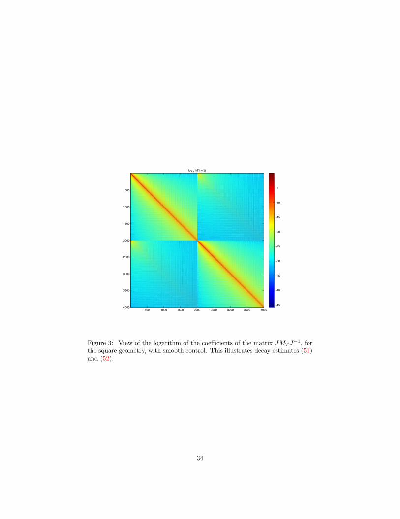
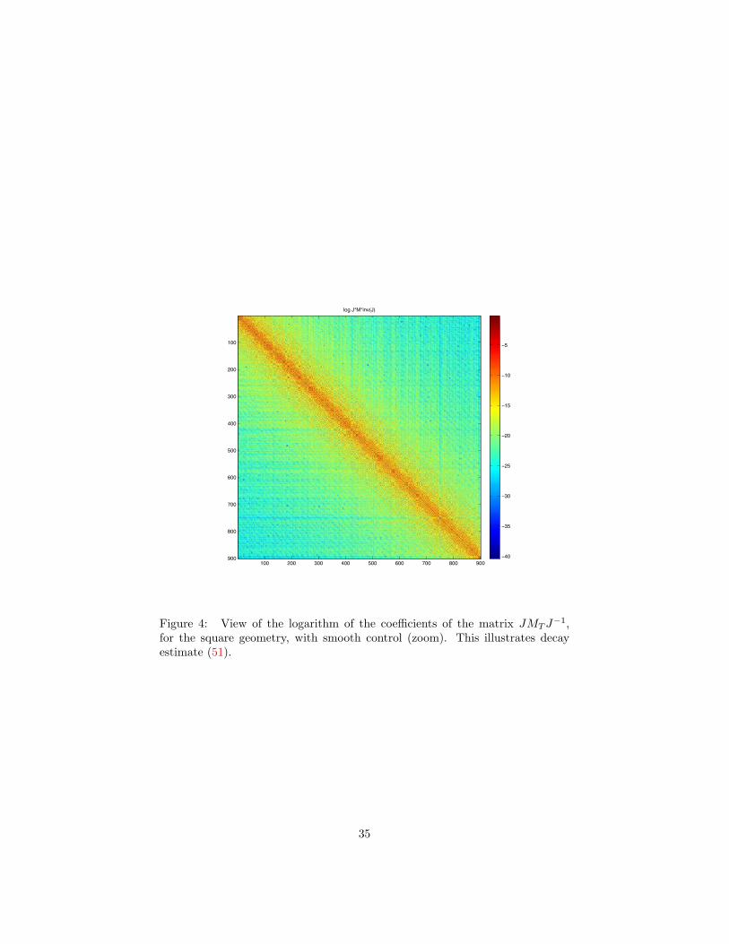
Figure 3 shows the log of JMT,ωJ−1 coefficients and illustrates the
decay estimates (51) and (52). A zoom in is done in figure 4, so that we
15
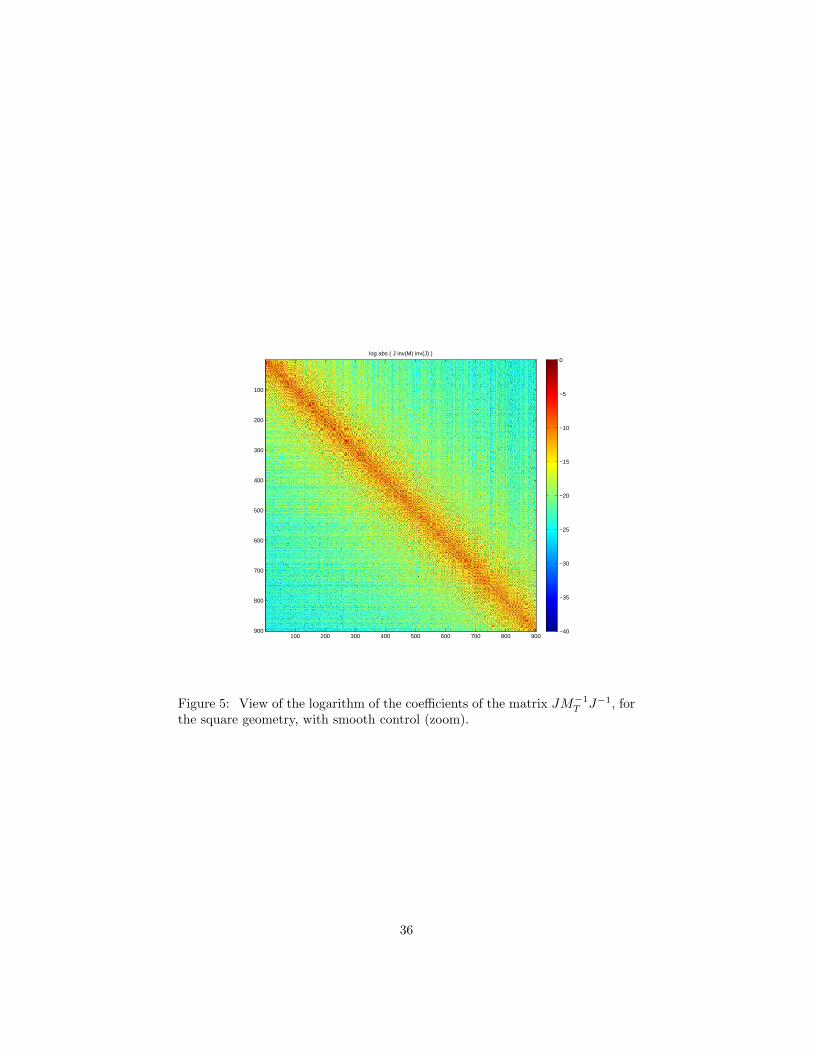
can observe more precisely (51). In particular we can notice that the dis-tribution of the coefficients along the diagonal of the matrix is not regular.Figure 5 presents the same zoom for JM−1
T,ωJ−1. This gives an illustration
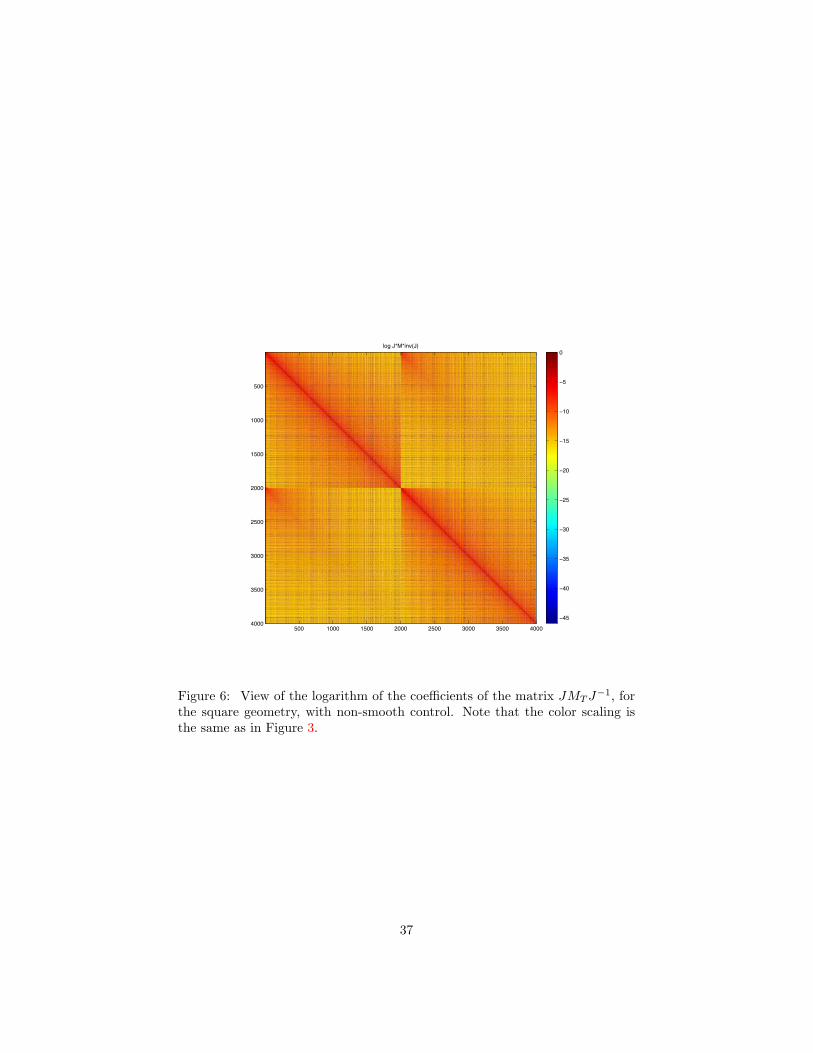
of the matrix structure of a microlocal operator. Figure 6 represents thelog of JMT,ωJ
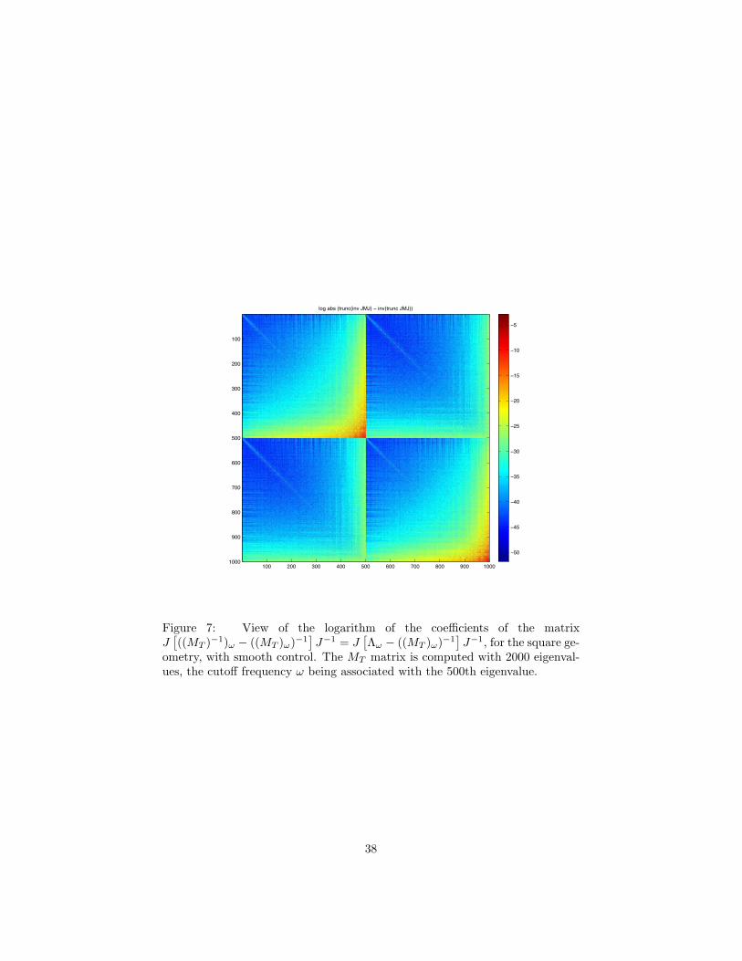
−1 coefficients without smoothing. And finally, figure 7 givesa view of the convergence of our Galerkin approximation, as it presentsthe matrix entries of J(Λω −M−1
T,ω)J−1, illustrating lemma 2, its proof,and lemma 3.
[Figure 3 about here.]
[Figure 4 about here.]
[Figure 5 about here.]
[Figure 6 about here.]
[Figure 7 about here.]
2.4 Computation of the discrete control operator
For any real ω, let N(ω) = supn, ωn ≤ ω. Then the dimension of thevector space L2
ω is equal toN(ω). Let us define the following (φj)1≤j≤2N(ω):(φj =
ej
ωjfor 1 ≤ j ≤ N(ω)
φj = ej−N(ω) for N(ω) + 1 ≤ j ≤ 2N(ω)(53)
Then (φj)1≤j≤2N(ω) is an orthonormal basis of the Hilbert space Hω =Πω(H1
0 (Ω)⊕ L2(Ω)).In this section we compute explicitly
`MTφl|φk
´H
for all 1 ≤ k, l ≤2N(ω). We recall
eisA»ei0
–=
»cos(sωi)ei(x)−ωi sin(sωi)ei(x)
–eisA
»0ei
–=
»sin(sωi)ei(x)/ωicos(sωi)ei(x)
– (54)
We now compute the coefficients of the MT matrix, namely MT n,m =`MTφn|φm
´H
:
MT n,m =`MTφn|φm
´H
=R T
0
`eisABB∗e−isAφn|φm
´Hdt
=R T
0
`„ 0 00 χ2
«e−isAφn|e−isAφm
´Hdt
(55)
We now have to distinguish four cases, depending on m,n being smaller
16
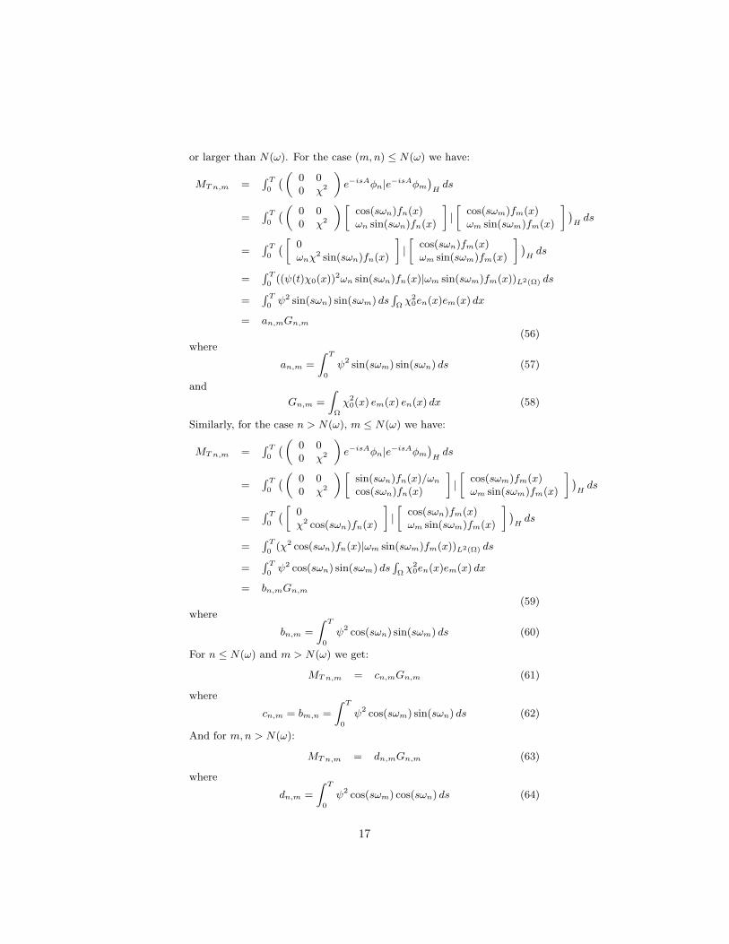
or larger than N(ω). For the case (m,n) ≤ N(ω) we have:
MT n,m =R T
0
`„ 0 00 χ2
«e−isAφn|e−isAφm
´Hds
=R T
0
`„ 0 00 χ2
«»cos(sωn)fn(x)ωn sin(sωn)fn(x)
–|»
cos(sωm)fm(x)ωm sin(sωm)fm(x)
– ´Hds
=R T
0
` » 0ωnχ
2 sin(sωn)fn(x)
–|»
cos(sωn)fm(x)ωm sin(sωm)fm(x)
– ´Hds
=R T
0((ψ(t)χ0(x))2ωn sin(sωn)fn(x)|ωm sin(sωm)fm(x))L2(Ω) ds
=R T
0ψ2 sin(sωn) sin(sωm) ds
RΩχ2
0en(x)em(x) dx
= an,mGn,m(56)
where
an,m =
Z T
0
ψ2 sin(sωm) sin(sωn) ds (57)
and
Gn,m =
ZΩ
χ20(x) em(x) en(x) dx (58)
Similarly, for the case n > N(ω), m ≤ N(ω) we have:
MT n,m =R T
0
`„ 0 00 χ2
«e−isAφn|e−isAφm
´Hds
=R T
0
`„ 0 00 χ2
«»sin(sωn)fn(x)/ωncos(sωn)fn(x)
–|»
cos(sωm)fm(x)ωm sin(sωm)fm(x)
– ´Hds
=R T
0
` » 0χ2 cos(sωn)fn(x)
–|»
cos(sωn)fm(x)ωm sin(sωm)fm(x)
– ´Hds
=R T
0(χ2 cos(sωn)fn(x)|ωm sin(sωm)fm(x))L2(Ω) ds
=R T
0ψ2 cos(sωn) sin(sωm) ds
RΩχ2
0en(x)em(x) dx
= bn,mGn,m(59)
where
bn,m =
Z T
0
ψ2 cos(sωn) sin(sωm) ds (60)
For n ≤ N(ω) and m > N(ω) we get:
MT n,m = cn,mGn,m (61)
where
cn,m = bm,n =
Z T
0
ψ2 cos(sωm) sin(sωn) ds (62)
And for m,n > N(ω):
MT n,m = dn,mGn,m (63)
where
dn,m =
Z T
0
ψ2 cos(sωm) cos(sωn) ds (64)
17
The above integrals have to be implemented carefully when |ωn − ωm| issmall, even when ψ(t) = 1.
3 Numerical setup and validation
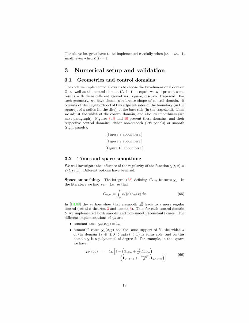
3.1 Geometries and control domains
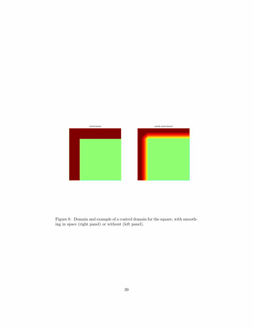
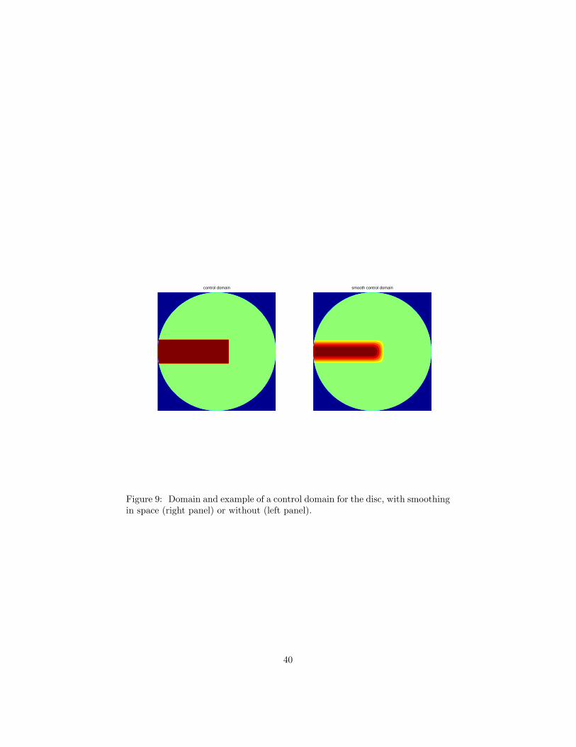
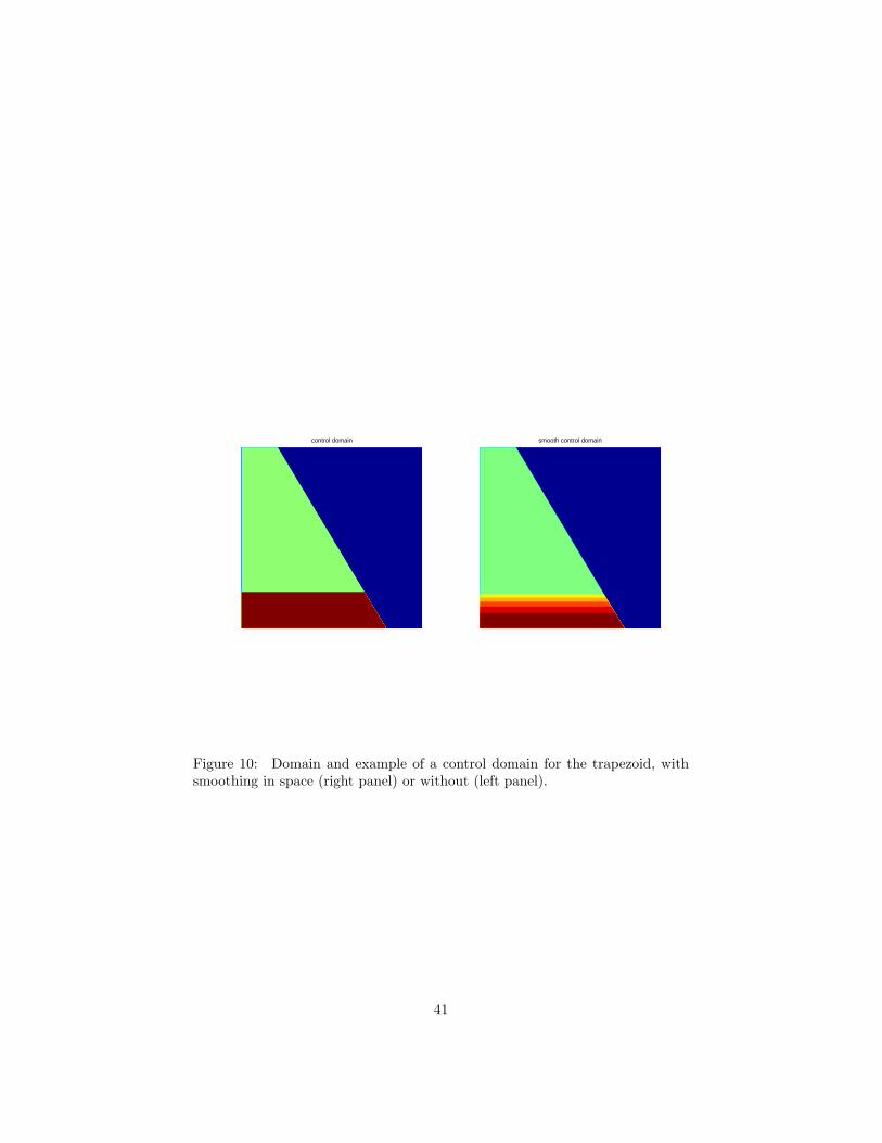
The code we implemented allows us to choose the two-dimensional domainΩ, as well as the control domain U . In the sequel, we will present someresults with three different geometries: square, disc and trapezoid. Foreach geometry, we have chosen a reference shape of control domain. Itconsists of the neighborhood of two adjacent sides of the boundary (in thesquare), of a radius (in the disc), of the base side (in the trapezoid). Thenwe adjust the width of the control domain, and also its smoothness (seenext paragraph). Figures 8, 9 and 10 present these domains, and theirrespective control domains, either non-smooth (left panels) or smooth(right panels).
[Figure 8 about here.]
[Figure 9 about here.]
[Figure 10 about here.]
3.2 Time and space smoothing
We will investigate the influence of the regularity of the function χ(t, x) =ψ(t)χ0(x). Different options have been set.
Space-smoothing. The integral (58) defining Gn,m features χ0. Inthe literature we find χ0 = 1U , so that
Gn,m =
ZU
en(x) em(x) dx (65)
In [DL09] the authors show that a smooth χ20 leads to a more regular
control (see also theorem 3 and lemma 3). Thus for each control domainU we implemented both smooth and non-smooth (constant) cases. Thedifferent implementations of χ0 are:
• constant case: χ0(x, y) = 1U ,
• “smooth” case: χ0(x, y) has the same support of U , the width aof the domain x ∈ Ω, 0 < χ0(x) < 1 is adjustable, and on thisdomain χ is a polynomial of degree 2. For example, in the squarewe have:
χ0(x, y) = 1Uh1−
“1x≥a + x2
a2.1x<a
”“1y≤1−a + (1−y)2
a2.1y>1−a
”i (66)
18
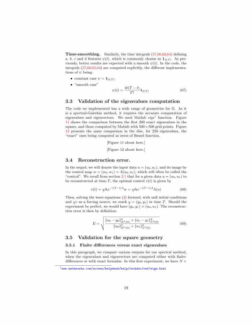
Time-smoothing. Similarly, the time integrals (57,60,62,64) defininga, b, c and d features ψ(t), which is commonly chosen as 1[0,T ]. As pre-viously, better results are expected with a smooth ψ(t). In the code, theintegrals (57,60,62,64) are computed explicitly, the different implementa-tions of ψ being:
• constant case ψ = 1[0,T ],
• “smooth case”
ψ(t) =4t(T − t)
T 21[0,T ] (67)
3.3 Validation of the eigenvalues computation
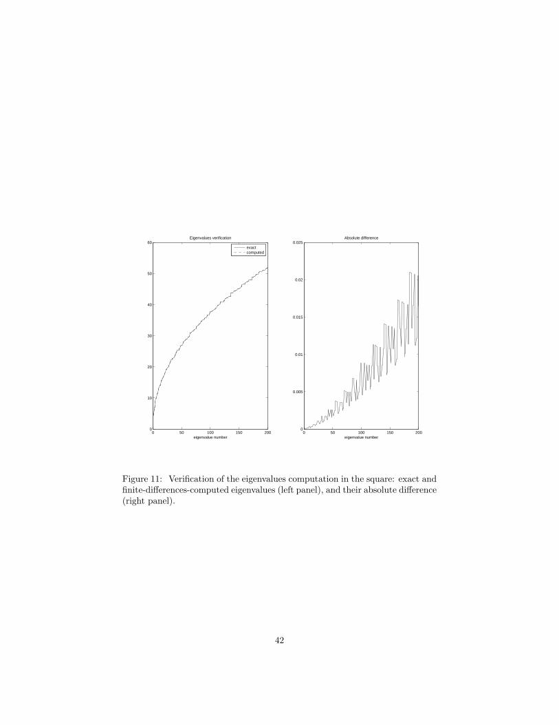
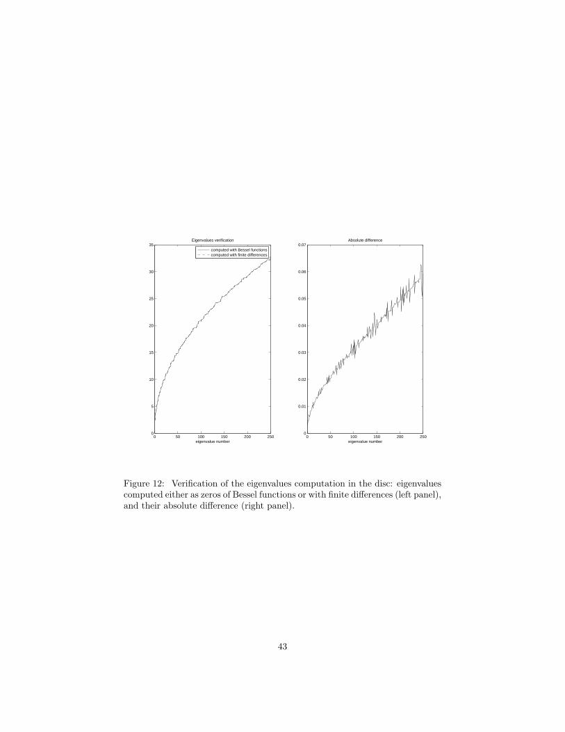
The code we implemented has a wide range of geometries for Ω. As itis a spectral-Galerkin method, it requires the accurate computation ofeigenvalues and eigenvectors. We used Matlab eigs1 function. Figure11 shows the comparison between the first 200 exact eigenvalues in thesquare, and those computed by Matlab with 500×500 grid-points. Figure12 presents the same comparison in the disc, for 250 eigenvalues, the“exact” ones being computed as zeros of Bessel function.
[Figure 11 about here.]
[Figure 12 about here.]
3.4 Reconstruction error.
In the sequel, we will denote the input data u = (u0, u1), and its image bythe control map w = (w0, w1) = Λ(u0, u1), which will often be called the“control”. We recall from section 2.1 that for a given data u = (u0, u1) tobe reconstructed at time T , the optimal control v(t) is given by
v(t) = χ∂te−i(T−t)Aw = χ∂te
−i(T−t)AΛ(u) (68)
Then, solving the wave equations (2) forward, with null initial conditionsand χv as a forcing source, we reach y = (y0, y1) in time T . Should theexperiment be perfect, we would have (y0, y1) = (u0, u1). The reconstruc-tion error is then by definition:
E =
vuut‖u0 − y0‖2H1(Ω)+ ‖u1 − y1‖2L2(Ω)
‖u0‖2H1(Ω)+ ‖u1‖2L2(Ω)
(69)
3.5 Validation for the square geometry
3.5.1 Finite differences versus exact eigenvalues
In this paragraph, we compare various outputs for our spectral method,when the eigenvalues and eigenvectors are computed either with finite-differences or with exact formulas. In this first experiment, we have N ×
1www.mathworks.com/access/helpdesk/help/techdoc/ref/eigs.html
19
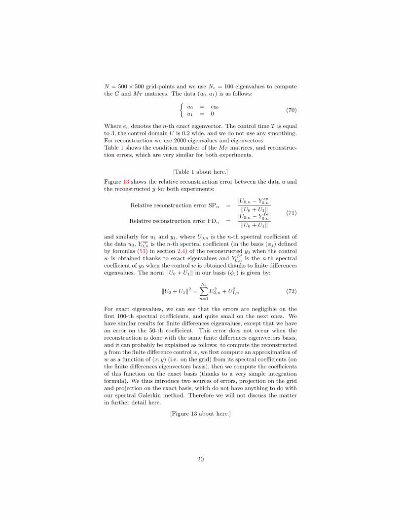
N = 500 × 500 grid-points and we use Ne = 100 eigenvalues to computethe G and MT matrices. The data (u0, u1) is as follows:
u0 = e50
u1 = 0(70)
Where en denotes the n-th exact eigenvector. The control time T is equalto 3, the control domain U is 0.2 wide, and we do not use any smoothing.For reconstruction we use 2000 eigenvalues and eigenvectors.Table 1 shows the condition number of the MT matrices, and reconstruc-tion errors, which are very similar for both experiments.
[Table 1 about here.]
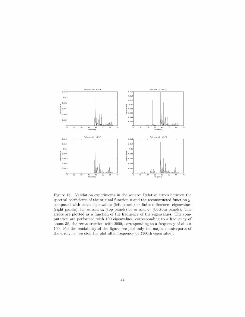
Figure 13 shows the relative reconstruction error between the data u andthe reconstructed y for both experiments:
Relative reconstruction error SPn =|U0,n − Y sp0,n|‖U0 + U1‖
Relative reconstruction error FDn =|U0,n − Y fd0,n|‖U0 + U1‖
(71)
and similarly for u1 and y1, where U0,n is the n-th spectral coefficient ofthe data u0, Y sp0,n is the n-th spectral coefficient (in the basis (φj) definedby formulas (53) in section 2.4) of the reconstructed y0 when the controlw is obtained thanks to exact eigenvalues and Y fd0,n is the n-th spectralcoefficient of y0 when the control w is obtained thanks to finite differenceseigenvalues. The norm ‖U0 + U1‖ in our basis (φj) is given by:
‖U0 + U1‖2 =
NeXn=1
U20,n + U2
1,n (72)
For exact eigenvalues, we can see that the errors are negligible on thefirst 100-th spectral coefficients, and quite small on the next ones. Wehave similar results for finite differences eigenvalues, except that we havean error on the 50-th coefficient. This error does not occur when thereconstruction is done with the same finite differences eigenvectors basis,and it can probably be explained as follows: to compute the reconstructedy from the finite difference control w, we first compute an approximation ofw as a function of (x, y) (i.e. on the grid) from its spectral coefficients (onthe finite differences eigenvectors basis), then we compute the coefficientsof this function on the exact basis (thanks to a very simple integrationformula). We thus introduce two sources of errors, projection on the gridand projection on the exact basis, which do not have anything to do withour spectral Galerkin method. Therefore we will not discuss the matterin further detail here.
[Figure 13 about here.]
20
3.5.2 Impact of the number of eigenvalues
In this paragraph, we still use the same data (70), but the number of eigen-values and eigenvectors Ne used to compute the MT matrices is varying.Table 2 shows MT condition numbers and reconstruction errors for variousNe with exact or finite-differences-computed eigenvalues. The reconstruc-tion is still performed with 2000 exact eigenvalues. We can see that thefinite differences eigenvalues lead to almost as good results as exact eigen-values. We also observe in both cases the decrease of the reconstructionerror with an increasing number of eigenvalues, as predicted in lemma 3.A 5% error is obtained with 70 eigenvalues (the input data being the 50-theigenvalue), and 100 eigenvalues lead to less than 2%.
[Table 2 about here.]
4 Numerical experiments
4.1 Frequency localization
In this subsection, the geometry (square) as well as the number of eigen-values used (200 for HUM, 2000 for verification) are fixed. Note also thatin this paragraph we use only exact eigenvalues for HUM and verification.The data is also fixed to a given eigenmode, that is:
u0 = e50 u1 = 0 (73)
where en is the n-th eigenvector of −∆ on the square.
[Figure 14 about here.]
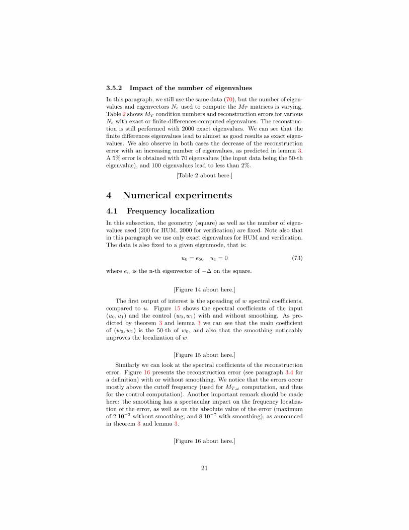
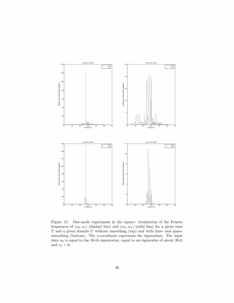
The first output of interest is the spreading of w spectral coefficients,compared to u. Figure 15 shows the spectral coefficients of the input(u0, u1) and the control (w0, w1) with and without smoothing. As pre-dicted by theorem 3 and lemma 3 we can see that the main coefficientof (w0, w1) is the 50-th of w0, and also that the smoothing noticeablyimproves the localization of w.
[Figure 15 about here.]
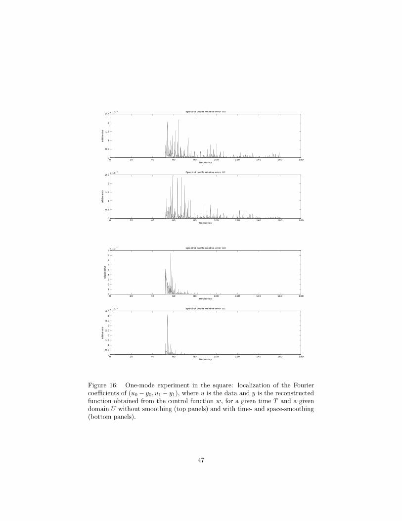
Similarly we can look at the spectral coefficients of the reconstructionerror. Figure 16 presents the reconstruction error (see paragraph 3.4 fora definition) with or without smoothing. We notice that the errors occurmostly above the cutoff frequency (used for MT,ω computation, and thusfor the control computation). Another important remark should be madehere: the smoothing has a spectacular impact on the frequency localiza-tion of the error, as well as on the absolute value of the error (maximumof 2.10−3 without smoothing, and 8.10−7 with smoothing), as announcedin theorem 3 and lemma 3.
[Figure 16 about here.]
21
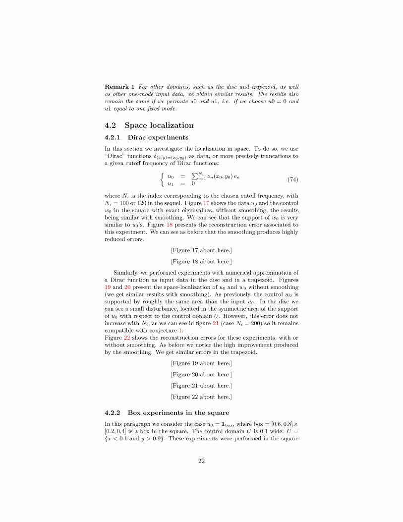
Remark 1 For other domains, such as the disc and trapezoid, as wellas other one-mode input data, we obtain similar results. The results alsoremain the same if we permute u0 and u1, i.e. if we choose u0 = 0 andu1 equal to one fixed mode.
4.2 Space localization
4.2.1 Dirac experiments
In this section we investigate the localization in space. To do so, we use“Dirac” functions δ(x,y)=(x0,y0) as data, or more precisely truncations toa given cutoff frequency of Dirac functions:
u0 =PNii=1 en(x0, y0) en
u1 = 0(74)
where Ni is the index corresponding to the chosen cutoff frequency, withNi = 100 or 120 in the sequel. Figure 17 shows the data u0 and the controlw0 in the square with exact eigenvalues, without smoothing, the resultsbeing similar with smoothing. We can see that the support of w0 is verysimilar to u0’s. Figure 18 presents the reconstruction error associated tothis experiment. We can see as before that the smoothing produces highlyreduced errors.
[Figure 17 about here.]
[Figure 18 about here.]
Similarly, we performed experiments with numerical approximation ofa Dirac function as input data in the disc and in a trapezoid. Figures19 and 20 present the space-localization of u0 and w0 without smoothing(we get similar results with smoothing). As previously, the control w0 issupported by roughly the same area than the input u0. In the disc wecan see a small disturbance, located in the symmetric area of the supportof u0 with respect to the control domain U . However, this error does notincrease with Ni, as we can see in figure 21 (case Ni = 200) so it remainscompatible with conjecture 1.Figure 22 shows the reconstruction errors for these experiments, with orwithout smoothing. As before we notice the high improvement producedby the smoothing. We get similar errors in the trapezoid.
[Figure 19 about here.]
[Figure 20 about here.]
[Figure 21 about here.]
[Figure 22 about here.]
4.2.2 Box experiments in the square
In this paragraph we consider the case u0 = 1box, where box = [0.6, 0.8]×[0.2, 0.4] is a box in the square. The control domain U is 0.1 wide: U =x < 0.1 and y > 0.9. These experiments were performed in the square
22
with 1000 exact eigenvalues for the MT matrix computation, the inputdata u0 being defined thanks to 800 eigenvalues. Figures 23 and 24 showthe space localization of the data u0 and the control w0 without andwith smoothing. As before we can notice that the space localization ispreserved, and that with smoothing the support of w0 is more sharplydefined. Figures 25 and 26 show the reconstruction errors for two differentdata, the first being the same as in figure 23, and the second being similarbut rotated by π/4. We show here only the case with smoothing, theerrors being larger but similarly shaped without. We can notice that theerrors lows and highs are located on a lattice whose axes are parallel tothe box sides. This is compatible with the structure of the wave-front setassociated to both input data.
[Figure 23 about here.]
[Figure 24 about here.]
[Figure 25 about here.]
[Figure 26 about here.]
4.3 Reconstruction error
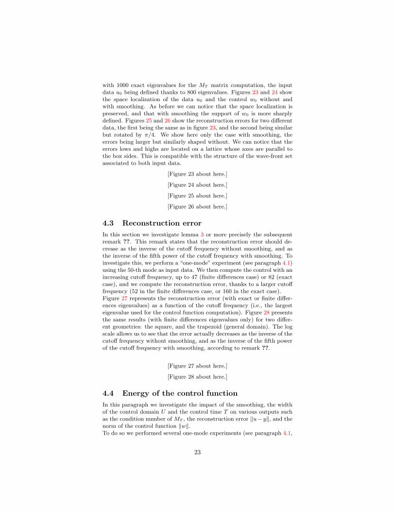
In this section we investigate lemma 3 or more precisely the subsequentremark ??. This remark states that the reconstruction error should de-crease as the inverse of the cutoff frequency without smoothing, and asthe inverse of the fifth power of the cutoff frequency with smoothing. Toinvestigate this, we perform a “one-mode” experiment (see paragraph 4.1)using the 50-th mode as input data. We then compute the control with anincreasing cutoff frequency, up to 47 (finite differences case) or 82 (exactcase), and we compute the reconstruction error, thanks to a larger cutofffrequency (52 in the finite differences case, or 160 in the exact case).Figure 27 represents the reconstruction error (with exact or finite differ-ences eigenvalues) as a function of the cutoff frequency (i.e., the largesteigenvalue used for the control function computation). Figure 28 presentsthe same results (with finite differences eigenvalues only) for two differ-ent geometries: the square, and the trapezoid (general domain). The logscale allows us to see that the error actually decreases as the inverse of thecutoff frequency without smoothing, and as the inverse of the fifth powerof the cutoff frequency with smoothing, according to remark ??.
[Figure 27 about here.]
[Figure 28 about here.]
4.4 Energy of the control function
In this paragraph we investigate the impact of the smoothing, the widthof the control domain U and the control time T on various outputs suchas the condition number of MT , the reconstruction error ‖u− y‖, and thenorm of the control function ‖w‖.To do so we performed several one-mode experiments (see paragraph 4.1,
23

mode 500) in the square, with exact eigenvalues, 1000 eigenvalues usedfor computation of MT , 2000 eigenvalues used for reconstruction and ver-ification. We chose various times: 2.5 and 8, plus their “smoothed” coun-terparts, according to the empirical formula Tsmooth = 15/8 ∗ T . Thisincrease of Tsmooth is justified on the theoretical level by formulas (31)and (30) which show that the efficiency of the control is related to a meanvalue of χ(t, x) on the trajectories. Similarly, we chose various width ofU : 1/10 and 3/10, plus their “smoothed” counterpart, which are double.Table 3 presents the numerical results for these experiments. This tabledraws several remarks. First, the condition number of MT , the recon-struction error and the norm of the control w decrease with increasingtime and U . Second, if we compare each non-smooth experiment with its“smoothed” counterpart (the comparison is of course approximate, sincethe “smoothed” time and width formulas are only reasonable approxima-tions), the condition number seems similar, as well as the norm of thecontrol function w, whereas the reconstruction error is far smaller withsmoothing than without.
[Table 3 about here.]
Figures 29 and 30 emphasize the impact of the control time, they presentthe reconstruction error, the norm of the control, and the condition num-ber of MT , as a function of the control time (varying between 2.5 and16), with or without smoothing. Conclusions are similar to the tableconclusions.
[Figure 29 about here.]
[Figure 30 about here.]
4.5 Condition number
In this section, we investigate conjecture 2. To do so, we compute thecondition number of MT,ω, as we have:
cond(MT,ω) = ‖MT,ω‖.‖M−1T,ω‖ ' ‖MT ‖.‖M−1
T,ω‖ (75)
Figure 31 shows the condition number of the MT matrix as a functionof the control time or of the last eigenvalue used for the control functioncomputation. According to conjecture 2, we obtain lines of the type
log (cond(MT,ω)) = ω.C(T,U) (76)
Figure 32 shows for various eigenvalues numbers the following curves:
T 7→ log (cond(MT,ω))
ω(77)
Similarly, we can draw conclusions compatible with conjecture 2, as thesecurves seems to converge when the number of eigenvalues grows to infinity.
[Figure 31 about here.]
[Figure 32 about here.]
24
4.6 Non-controlling domains
In this section we investigate two special experiments with non-controllingdomains, i.e. such that the geometric control condition is not satisfiedwhatever the control time.First we consider the domain presented in Figure 33.
[Figure 33 about here.]
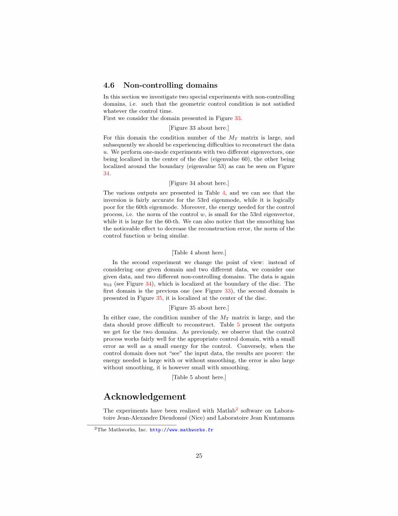
For this domain the condition number of the MT matrix is large, andsubsequently we should be experiencing difficulties to reconstruct the datau. We perform one-mode experiments with two different eigenvectors, onebeing localized in the center of the disc (eigenvalue 60), the other beinglocalized around the boundary (eigenvalue 53) as can be seen on Figure34.
[Figure 34 about here.]
The various outputs are presented in Table 4, and we can see that theinversion is fairly accurate for the 53rd eigenmode, while it is logicallypoor for the 60th eigenmode. Moreover, the energy needed for the controlprocess, i.e. the norm of the control w, is small for the 53rd eigenvector,while it is large for the 60-th. We can also notice that the smoothing hasthe noticeable effect to decrease the reconstruction error, the norm of thecontrol function w being similar.
[Table 4 about here.]
In the second experiment we change the point of view: instead ofconsidering one given domain and two different data, we consider onegiven data, and two different non-controlling domains. The data is againu53 (see Figure 34), which is localized at the boundary of the disc. Thefirst domain is the previous one (see Figure 33), the second domain ispresented in Figure 35, it is localized at the center of the disc.
[Figure 35 about here.]
In either case, the condition number of the MT matrix is large, and thedata should prove difficult to reconstruct. Table 5 present the outputswe get for the two domains. As previously, we observe that the controlprocess works fairly well for the appropriate control domain, with a smallerror as well as a small energy for the control. Conversely, when thecontrol domain does not “see” the input data, the results are poorer: theenergy needed is large with or without smoothing, the error is also largewithout smoothing, it is however small with smoothing.
[Table 5 about here.]
Acknowledgement
The experiments have been realized with Matlab2 software on Labora-toire Jean-Alexandre Dieudonne (Nice) and Laboratoire Jean Kuntzmann
2The Mathworks, Inc. http://www.mathworks.fr
25
(Grenoble) computing machines. The INRIA Gforge3 has also been used.The authors thank J.-M. Lacroix (Laboratoire J.-A. Dieudonne) for hismanaging of Nice computing machine.This work has been partially supported by Institut Universitaire de France.
References
[AL98] M. Asch and G. Lebeau. Geometrical aspects of exact bound-ary controllability of the wave equation. a numerical study.ESAIM:COCV, 3:163–212, 1998. 3
[BL01] N. Burq and G. Lebeau. Mesures de defaut de compacite, ap-plication au systeme de lame. Ann. Sci. Ecole Norm. Sup.,34(6):817–870, 2001. 12
[BLR92] C. Bardos, G. Lebeau, and J. Rauch. Sharp sufficient conditionsfor the observation, control and stabilisation of waves from theboundary. SIAM J.Control Optim., 305:1024–1065, 1992. 3, 8,10
[DL09] B. Dehman and G. Lebeau. Analysis of the HUM Control Oper-ator and Exact Controllability for Semilinear Waves in UniformTime. to appear in SIAM Control and Optimization, 2009. 8,9, 10, 15, 18
[Ger91] P. Gerard. Microlocal defect measures. C.P.D.E, 16:1762–1794,1991. 12
[GHL08] R. Glowinski, J. W. He, and J.-L. Lions. Exact and ApproximateControllability for Distributed Parameter Systems: A NumericalApproach. Cambridge University Press, 2008. 3
[GLL90] R. Glowinski, C.H. Li, and J.L. Lions. A numerical approachto the exact boundary controllability of the wave equation (I).dirichlet controls : description of the numerical methods. JapanJ. Appl. Math., 7:1–76, 1990. 3
[Hor85] L. Hormander. The analysis of linear partial differential op-erators. III. Grundl. Math. Wiss. Band 274. Springer-Verlag,Berlin, 1985. Pseudodifferential operators. 8, 10, 11
[Leb92] G. Lebeau. Controle analytique I : Estimations a priori. DukeMath. J., 68(1):1–30, 1992. 14
[Lio88] J.-L. Lions. Controlabilite exacte, perturbations et stabilisa-tion de systemes distribues. Tome 2, volume 9 of Recherches enMathematiques Appliquees [Research in Applied Mathematics].Masson, Paris, 1988. 3, 5
[MS78] R.-B. Melrose and J. Sjostrand. Singularities of boundary valueproblems I. CPAM, 31:593–617, 1978. 3, 8, 10
[MS82] R.-B. Melrose and J. Sjostrand. Singularities of boundary valueproblems II. CPAM, 35:129–168, 1982. 3, 8, 10
3http://gforge.inria.fr
26
[Rus78] D.-L. Russell. Controllability and stabilizability theory for lin-ear partial differential equations: recent progress and open ques-tions. SIAM Rev, 20:639–739, 1978. 3
[Tay81] M. Taylor. Pseudodifferential operators. Princeton UniversityPress, 1981. 10
[Zua02] E. Zuazua. Controllability of partial differential equations andits semi-discrete approximations. Discrete and Continuous Dy-namical Systems, 8(2):469–513, 2002. 3
[Zua05] E. Zuazua. Propagation, observation, and control of waves ap-proximated by finite difference methods. SIAM Rev, 47(2):197–243, 2005. 3
27
List of Figures
1 Example of optical rays. . . . . . . . . . . . . . . . . 322 Example of optical ray with only transversal reflection
points. . . . . . . . . . . . . . . . . . . . . . . . . . . 333 View of the logarithm of the coefficients of the ma-
trix JMT J−1, for the square geometry, with smoothcontrol. This illustrates decay estimates (51) and (52). 34
4 View of the logarithm of the coefficients of the ma-trix JMT J−1, for the square geometry, with smoothcontrol (zoom). This illustrates decay estimate (51). 35
5 View of the logarithm of the coefficients of the ma-trix JM−1
T J−1, for the square geometry, with smoothcontrol (zoom). . . . . . . . . . . . . . . . . . . . . . 36
6 View of the logarithm of the coefficients of the matrixJMT J−1, for the square geometry, with non-smoothcontrol. Note that the color scaling is the same as inFigure 3. . . . . . . . . . . . . . . . . . . . . . . . . . 37
7 View of the logarithm of the coefficients of the matrixJ
[((MT )−1)ω − ((MT )ω)−1
]J−1 = J
[Λω − ((MT )ω)−1
]J−1,
for the square geometry, with smooth control. TheMT matrix is computed with 2000 eigenvalues, thecutoff frequency ω being associated with the 500theigenvalue. . . . . . . . . . . . . . . . . . . . . . . . . 38
8 Domain and example of a control domain for the square,with smoothing in space (right panel) or without (leftpanel). . . . . . . . . . . . . . . . . . . . . . . . . . . 39
9 Domain and example of a control domain for the disc,with smoothing in space (right panel) or without (leftpanel). . . . . . . . . . . . . . . . . . . . . . . . . . . 40
10 Domain and example of a control domain for the trape-zoid, with smoothing in space (right panel) or without(left panel). . . . . . . . . . . . . . . . . . . . . . . . 41
11 Verification of the eigenvalues computation in the square:exact and finite-differences-computed eigenvalues (leftpanel), and their absolute difference (right panel). . 42
12 Verification of the eigenvalues computation in the disc:eigenvalues computed either as zeros of Bessel func-tions or with finite differences (left panel), and theirabsolute difference (right panel). . . . . . . . . . . . 43
28
13 Validation experiments in the square: Relative er-rors between the spectral coefficients of the originalfunction u and the reconstructed function y, com-puted with exact eigenvalues (left panels) or finitedifferences eigenvalues (right panels), for u0 and y0
(top panels) or u1 and y1 (bottom panels). The er-rors are plotted as a function of the frequency of theeigenvalues. The computation are performed with 100eigenvalues, corresponding to a frequency of about 38,the reconstruction with 2000, corresponding to a fre-quency of about 160. For the readability of the figure,we plot only the major counterparts of the error, i.e.we stop the plot after frequency 63 (300th eigenvalue). 44
14 Representation on the grid in 3D (left panel) or con-tour plot (right panel) of the 50-th eigenvector in thesquare. . . . . . . . . . . . . . . . . . . . . . . . . . . 45
15 One-mode experiment in the square: localization ofthe Fourier frequences of (u0, u1) (dashed line) and(w0, w1) (solid line) for a given time T and a given do-main U without smoothing (top) and with time- andspace-smoothing (bottom). The x-coordinate repre-sents the eigenvalues. The input data u0 is equal tothe 50-th eigenvector, equal to an eigenvalue of about26.8, and u1 = 0. . . . . . . . . . . . . . . . . . . . . 46
16 One-mode experiment in the square: localization ofthe Fourier coefficients of (u0−y0, u1−y1), where u isthe data and y is the reconstructed function obtainedfrom the control function w, for a given time T and agiven domain U without smoothing (top panels) andwith time- and space-smoothing (bottom panels). . . 47
17 Space localization of the data u0 (top panels) and thecontrol w0 (bottom panels), for a Dirac experimentin the square, with exact eigenvalues. These plotscorrespond to an experiment without smoothing, butit is similar with smoothing. Left panels represent 3Dview, and right panels show contour plots. . . . . . . 48
18 Difference between the data u0 and the reconstructedfunction y0 without smoothing (top panels) and withsmoothing (bottom panels) for a dirac experiment inthe square, with exact eigenvalues. Left panels repre-sent 3D view, and right panels show contour plots. . 49
29
19 Space localization of the data u0 (top panels) and thecontrol w0 (bottom panels), for a dirac experiment inthe disc. These plots correspond to an experimentwithout smoothing, but it is similar with smoothing.Left panels represent 3D view, and right panels showcontour plots. In this experiment, the input data isdefined with Ni = 100 eigenvectors. . . . . . . . . . 50
20 Space localization of the data u0 (top panels) and thecontrol w0 (bottom panels), for a dirac experimentin the trapezoid. These plots correspond to an ex-periment without smoothing, but it is similar withsmoothing. Left panels represent 3D view, and rightpanels show contour plots. In this experiment, theinput data is defined with Ni = 120 eigenvectors. . . 51
21 Space localization of the data u0 (top panels) and thecontrol w0 (bottom panels), for a dirac experiment inthe disc. These plots correspond to an experimentwith smoothing, and it is similar without smoothing.Left panels represent 3D view, and right panels showcontour plots. In this experiment, the input data isdefined with Ni = 200 eigenvectors. . . . . . . . . . . 52
22 Difference between the data u0 and the reconstructedfunction y0 for a dirac experiment in the disc with-out smoothing (top panels) and with time- and space-smoothing (bottom panels). Left panels represent 3Dview, and right panels show contour plots. In thisexperiment, the input data is defined with Ni = 100eigenvectors. . . . . . . . . . . . . . . . . . . . . . . 53
23 Space localization of the control function w0 (bottompanels) with respect to the data u0 (top panels), inthe square, without smoothing: 3D plots on the left,and contour plots on the right. . . . . . . . . . . . . 54
24 Space localization of the control function w0 (bottompanels) with respect to the data u0 (top panels), inthe square, with smoothing. Left panels represent 3Dview, and right panels show contour plots. . . . . . . 55
25 Difference between the data u0 and the reconstructedfunction y0 (top panels) and u1 and y1 (bottom pan-els) with smoothing in the square. The data is theidentity function of a square whose edges are parallelto the x and y axes. Left panels represent 3D view,and right panels show contour plots. . . . . . . . . . 56
30
26 Difference between the data u0 and the reconstructedfunction y0 (top panels) and u1 and y1 (bottom pan-els) with smoothing in the square. The data is theidentity function of a square whose edges are parallelto the diagonals of the square. Left panels represent3D view, and right panels show contour plots. . . . . 57
27 Reconstruction errors for the finite differences and ex-act methods, as a function of the cutoff frequency (i.e.,the largest eigenvalue used for the control computa-tion), with or without time- and space-smoothing. . 58
28 Reconstruction errors for the finite differences method,in the square and in the trapezoid, as a function ofthe cutoff frequency (i.e., the largest eigenvalue usedfor the control computation), with or without time-and space-smoothing. . . . . . . . . . . . . . . . . . 59
29 Experiments in the square, with exact eigenvalues:impact of the smoothing on the reconstruction error(top) and on the norm of the control function (bot-tom), as a function of the control time. . . . . . . . 60
30 Experiments in the square, with exact eigenvalues:impact of the smoothing on the condition number ofthe MT matrix, as a function of the control time. . 61
31 Condition number of the MT,ω matrix as a functionof the cutoff frequency ω for various control times. . 62
32 Ratio of the log of the condition number of the MT,ω
matrix and the cutoff frequency ω, as a function ofthe control time for various eigenvalues numbers. . 63
33 Non-controlling domain U without (left) or with (right)smoothing. This domain consists of the neighborhoodof a radius which is truncated around the disc boundary. 64
34 Special modes chosen for experiment with non-controllingdomains, corresponding to the 53rd and 60th eigen-values. . . . . . . . . . . . . . . . . . . . . . . . . . 65
35 Non-controlling domain U without (left) or with (right)smoothing. This domain consists of the neighborhoodof a radius which is truncated around the disc center. 66
31
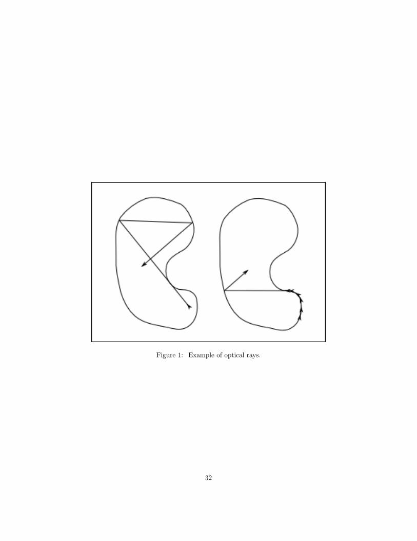
Figure 1: Example of optical rays.
32
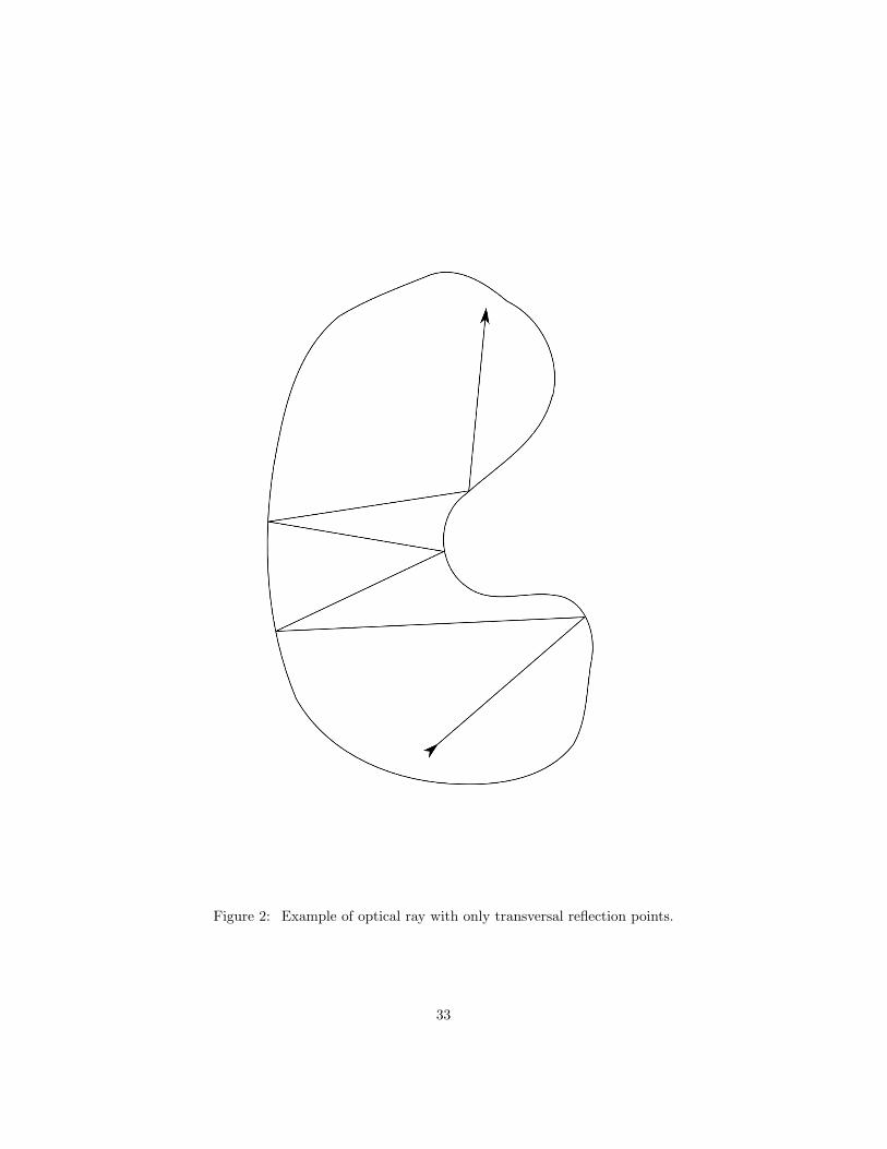
Figure 2: Example of optical ray with only transversal reflection points.
33
log J*M*inv(J)
500 1000 1500 2000 2500 3000 3500 4000
500
1000
1500
2000
2500
3000
3500
4000−45
−40
−35
−30
−25
−20
−15
−10
−5
Figure 3: View of the logarithm of the coefficients of the matrix JMT J−1, forthe square geometry, with smooth control. This illustrates decay estimates (51)and (52).
34
log J*M*inv(J)
100 200 300 400 500 600 700 800 900
100
200
300
400
500
600
700
800
900 −40
−35
−30
−25
−20
−15
−10
−5
Figure 4: View of the logarithm of the coefficients of the matrix JMT J−1,for the square geometry, with smooth control (zoom). This illustrates decayestimate (51).
35
log abs ( J inv(M) inv(J) )
100 200 300 400 500 600 700 800 900
100
200
300
400
500
600
700
800
900 −40
−35
−30
−25
−20
−15
−10
−5
0
Figure 5: View of the logarithm of the coefficients of the matrix JM−1T J−1, for
the square geometry, with smooth control (zoom).
36
log J*M*inv(J)
500 1000 1500 2000 2500 3000 3500 4000
500
1000
1500
2000
2500
3000
3500
4000−45
−40
−35
−30
−25
−20
−15
−10
−5
0
Figure 6: View of the logarithm of the coefficients of the matrix JMT J−1, forthe square geometry, with non-smooth control. Note that the color scaling isthe same as in Figure 3.
37
log abs (trunc(inv JMJ) − inv(trunc JMJ))
100 200 300 400 500 600 700 800 900 1000
100
200
300
400
500
600
700
800
900
1000−50
−45
−40
−35
−30
−25
−20
−15
−10
−5
Figure 7: View of the logarithm of the coefficients of the matrixJ
[((MT )−1)ω − ((MT )ω)−1
]J−1 = J
[Λω − ((MT )ω)−1
]J−1, for the square ge-
ometry, with smooth control. The MT matrix is computed with 2000 eigenval-ues, the cutoff frequency ω being associated with the 500th eigenvalue.
38
control domain smooth control domain
Figure 8: Domain and example of a control domain for the square, with smooth-ing in space (right panel) or without (left panel).
39
control domain smooth control domain
Figure 9: Domain and example of a control domain for the disc, with smoothingin space (right panel) or without (left panel).
40
control domain smooth control domain
Figure 10: Domain and example of a control domain for the trapezoid, withsmoothing in space (right panel) or without (left panel).
41
0 50 100 150 2000
10
20
30
40
50
60
eigenvalue number
Eigenvalues verification
exactcomputed
0 50 100 150 2000
0.005
0.01
0.015
0.02
0.025
eigenvalue number
Absolute difference
Figure 11: Verification of the eigenvalues computation in the square: exact andfinite-differences-computed eigenvalues (left panel), and their absolute difference(right panel).
42
0 50 100 150 200 2500
5
10
15
20
25
30
35
eigenvalue number
Eigenvalues verification
computed with Bessel functionscomputed with finite differences
0 50 100 150 200 2500
0.01
0.02
0.03
0.04
0.05
0.06
0.07
eigenvalue number
Absolute difference
Figure 12: Verification of the eigenvalues computation in the disc: eigenvaluescomputed either as zeros of Bessel functions or with finite differences (left panel),and their absolute difference (right panel).
43
0 10 20 30 40 50 60 700
0.002
0.004
0.006
0.008
0.01
0.012
frequency
rela
tive
erro
r
Rel. error U0 − Y0 SP
0 10 20 30 40 50 60 700
0.002
0.004
0.006
0.008
0.01
0.012
0.014
0.016
frequency
rela
tive
erro
r
Rel. error U0 − Y0 FD
0 10 20 30 40 50 60 700
0.002
0.004
0.006
0.008
0.01
0.012
0.014
frequency
rela
tive
erro
r
Rel. error U1 − Y1 SP
0 10 20 30 40 50 60 700
0.002
0.004
0.006
0.008
0.01
0.012
0.014
frequency
rela
tive
erro
r
Rel. error U1 − Y1 FD
Figure 13: Validation experiments in the square: Relative errors between thespectral coefficients of the original function u and the reconstructed function y,computed with exact eigenvalues (left panels) or finite differences eigenvalues(right panels), for u0 and y0 (top panels) or u1 and y1 (bottom panels). Theerrors are plotted as a function of the frequency of the eigenvalues. The com-putation are performed with 100 eigenvalues, corresponding to a frequency ofabout 38, the reconstruction with 2000, corresponding to a frequency of about160. For the readability of the figure, we plot only the major counterparts ofthe error, i.e. we stop the plot after frequency 63 (300th eigenvalue).
44
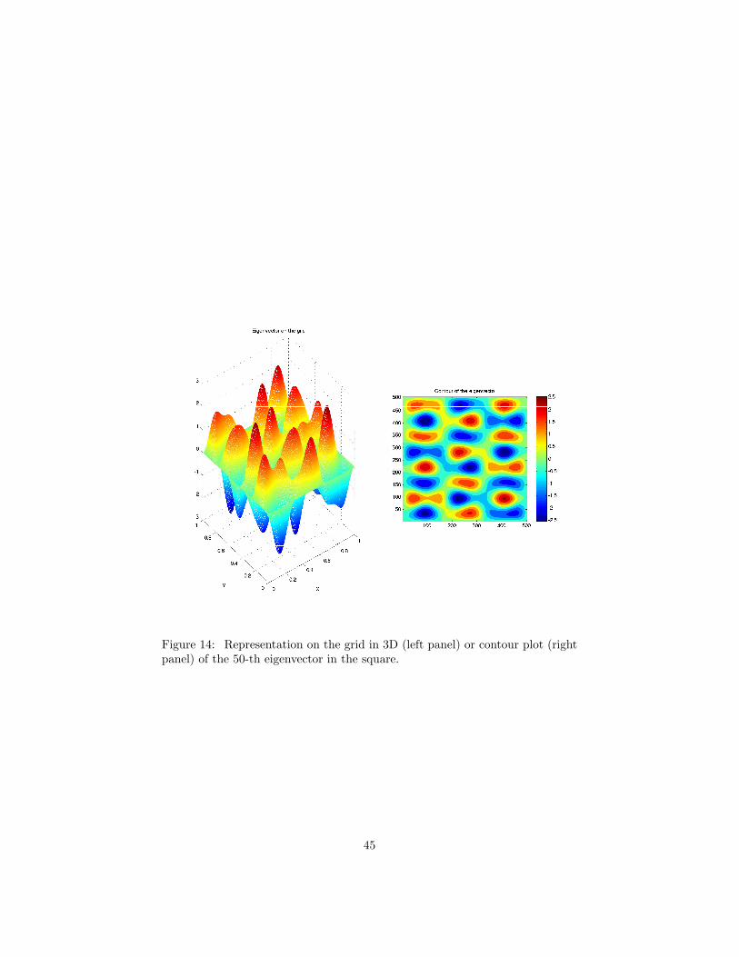
Figure 14: Representation on the grid in 3D (left panel) or contour plot (rightpanel) of the 50-th eigenvector in the square.
45
0 10 20 30 40 50 600
20
40
60
80
100
120
140
frequency
abso
lute
val
ue o
f the
spe
ctra
l coe
fficie
nt
Spectral coeffs
W0U0
0 10 20 30 40 50 600
5
10
15
20
25
frequency
abso
lute
val
ue o
f the
spe
ctra
l coe
fficie
nt
Spectral coeffs
W1U1
0 10 20 30 40 50 600
20
40
60
80
100
120
140
160
frequency
abso
lute
val
ue o
f the
spe
ctra
l coe
fficie
nt
Spectral coeffs
W0U0
0 10 20 30 40 50 600
2
4
6
8
10
12
frequency
abso
lute
val
ue o
f the
spe
ctra
l coe
fficie
nt
Spectral coeffs
W1U1
Figure 15: One-mode experiment in the square: localization of the Fourierfrequences of (u0, u1) (dashed line) and (w0, w1) (solid line) for a given timeT and a given domain U without smoothing (top) and with time- and space-smoothing (bottom). The x-coordinate represents the eigenvalues. The inputdata u0 is equal to the 50-th eigenvector, equal to an eigenvalue of about 26.8,and u1 = 0.
46
0 20 40 60 80 100 120 140 160 1800
0.5
1
1.5
2
2.5x 10
−3
frequency
rela
tive
erro
r
Spectral coeffs relative error U0
0 20 40 60 80 100 120 140 160 1800
0.5
1
1.5
2
2.5x 10
−3
frequency
rela
tive
erro
r
Spectral coeffs relative error U1
0 20 40 60 80 100 120 140 160 1800
1
2
3
4
5
6
7
8
9x 10
−7
frequency
rela
tive
erro
r
Spectral coeffs relative error U0
0 20 40 60 80 100 120 140 160 1800
0.5
1
1.5
2
2.5
3
3.5
4
4.5x 10
−6
frequency
rela
tive
erro
r
Spectral coeffs relative error U1
Figure 16: One-mode experiment in the square: localization of the Fouriercoefficients of (u0 − y0, u1 − y1), where u is the data and y is the reconstructedfunction obtained from the control function w, for a given time T and a givendomain U without smoothing (top panels) and with time- and space-smoothing(bottom panels).
47
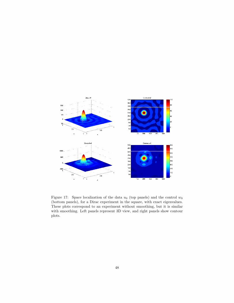
Figure 17: Space localization of the data u0 (top panels) and the control w0
(bottom panels), for a Dirac experiment in the square, with exact eigenvalues.These plots correspond to an experiment without smoothing, but it is similarwith smoothing. Left panels represent 3D view, and right panels show contourplots.
48
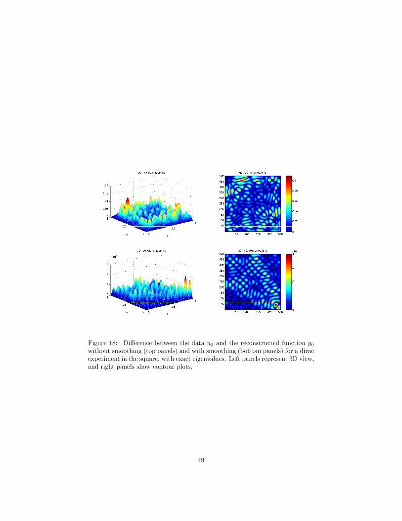
Figure 18: Difference between the data u0 and the reconstructed function y0
without smoothing (top panels) and with smoothing (bottom panels) for a diracexperiment in the square, with exact eigenvalues. Left panels represent 3D view,and right panels show contour plots.
49
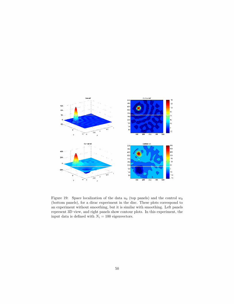
Figure 19: Space localization of the data u0 (top panels) and the control w0
(bottom panels), for a dirac experiment in the disc. These plots correspond toan experiment without smoothing, but it is similar with smoothing. Left panelsrepresent 3D view, and right panels show contour plots. In this experiment, theinput data is defined with Ni = 100 eigenvectors.
50

Figure 20: Space localization of the data u0 (top panels) and the control w0
(bottom panels), for a dirac experiment in the trapezoid. These plots corre-spond to an experiment without smoothing, but it is similar with smoothing.Left panels represent 3D view, and right panels show contour plots. In thisexperiment, the input data is defined with Ni = 120 eigenvectors.
51
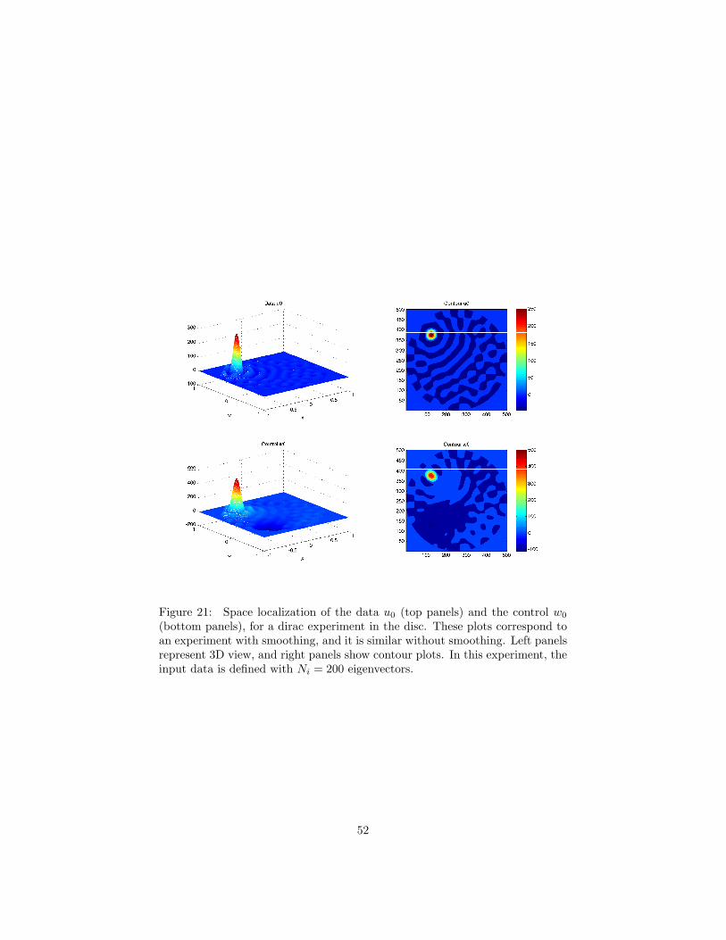
Figure 21: Space localization of the data u0 (top panels) and the control w0
(bottom panels), for a dirac experiment in the disc. These plots correspond toan experiment with smoothing, and it is similar without smoothing. Left panelsrepresent 3D view, and right panels show contour plots. In this experiment, theinput data is defined with Ni = 200 eigenvectors.
52
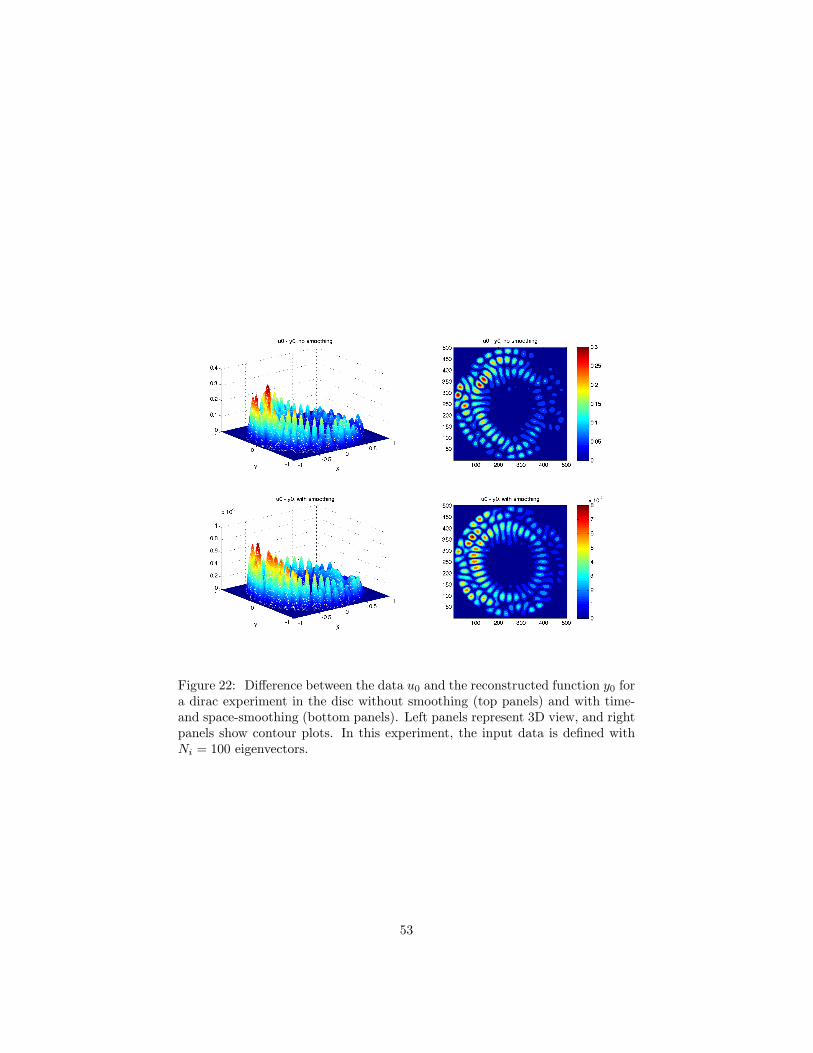
Figure 22: Difference between the data u0 and the reconstructed function y0 fora dirac experiment in the disc without smoothing (top panels) and with time-and space-smoothing (bottom panels). Left panels represent 3D view, and rightpanels show contour plots. In this experiment, the input data is defined withNi = 100 eigenvectors.
53
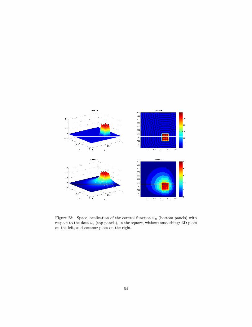
Figure 23: Space localization of the control function w0 (bottom panels) withrespect to the data u0 (top panels), in the square, without smoothing: 3D plotson the left, and contour plots on the right.
54
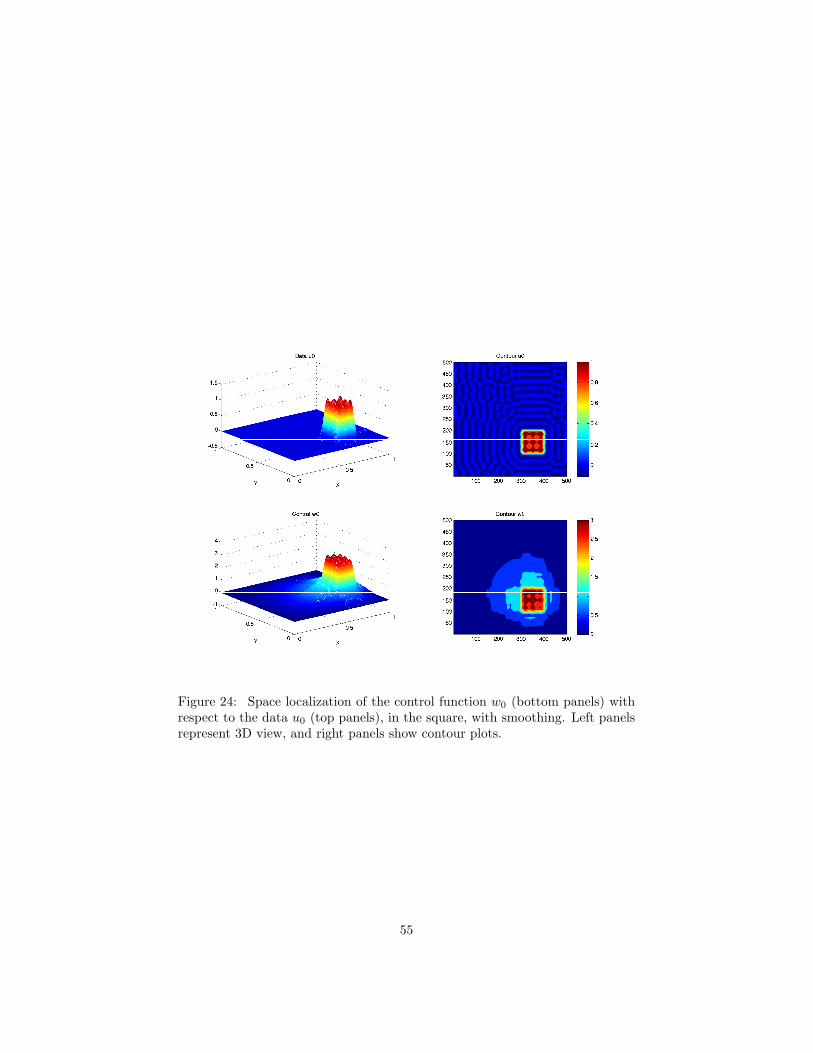
Figure 24: Space localization of the control function w0 (bottom panels) withrespect to the data u0 (top panels), in the square, with smoothing. Left panelsrepresent 3D view, and right panels show contour plots.
55
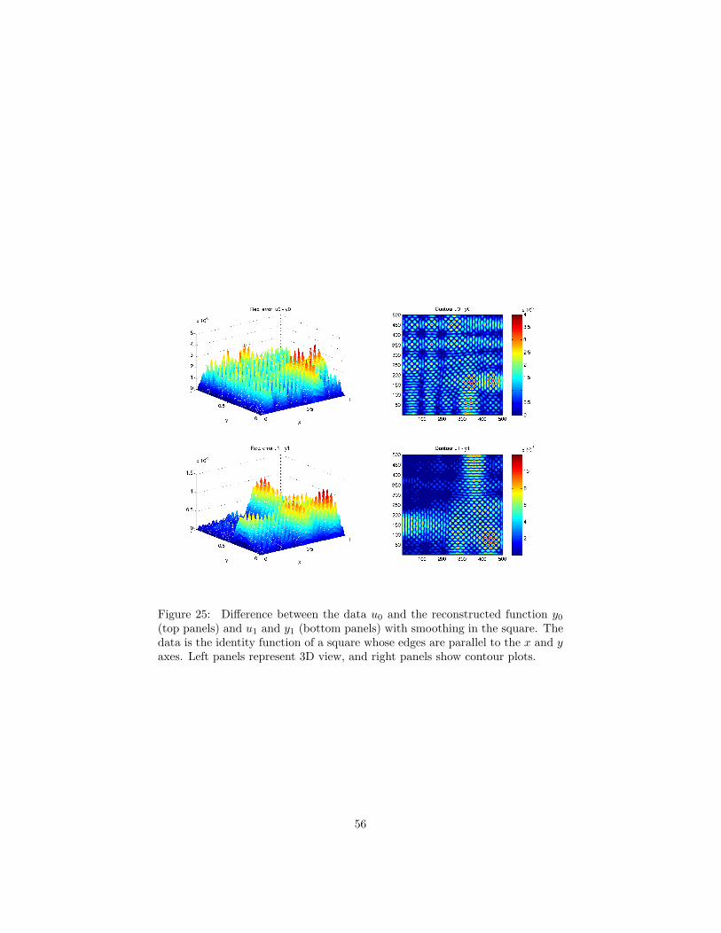
Figure 25: Difference between the data u0 and the reconstructed function y0
(top panels) and u1 and y1 (bottom panels) with smoothing in the square. Thedata is the identity function of a square whose edges are parallel to the x and yaxes. Left panels represent 3D view, and right panels show contour plots.
56
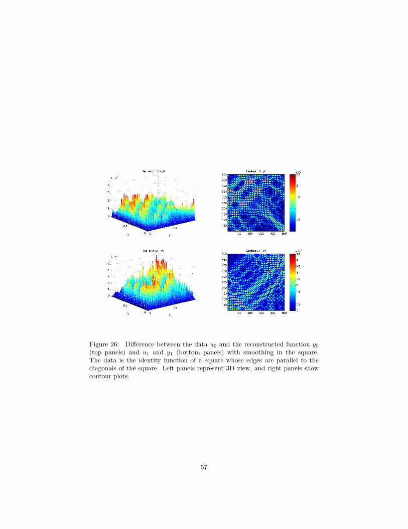
Figure 26: Difference between the data u0 and the reconstructed function y0
(top panels) and u1 and y1 (bottom panels) with smoothing in the square.The data is the identity function of a square whose edges are parallel to thediagonals of the square. Left panels represent 3D view, and right panels showcontour plots.
57
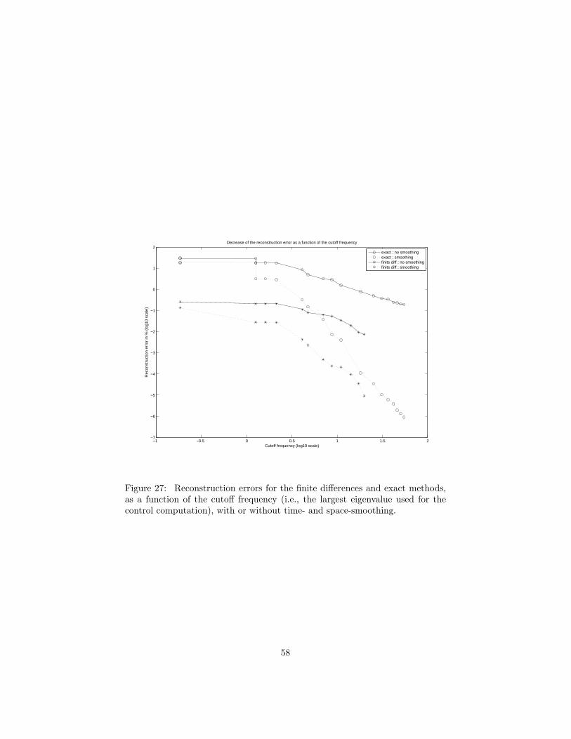
−1 −0.5 0 0.5 1 1.5 2−7
−6
−5
−4
−3
−2
−1
0
1
2
Cutoff frequency (log10 scale)
Rec
onst
ruct
ion
erro
r in
% (
log1
0 sc
ale)
Decrease of the reconstruction error as a function of the cutoff frequency
exact ; no smoothingexact ; smoothingfinite diff ; no smoothingfinite diff ; smoothing
Figure 27: Reconstruction errors for the finite differences and exact methods,as a function of the cutoff frequency (i.e., the largest eigenvalue used for thecontrol computation), with or without time- and space-smoothing.
58
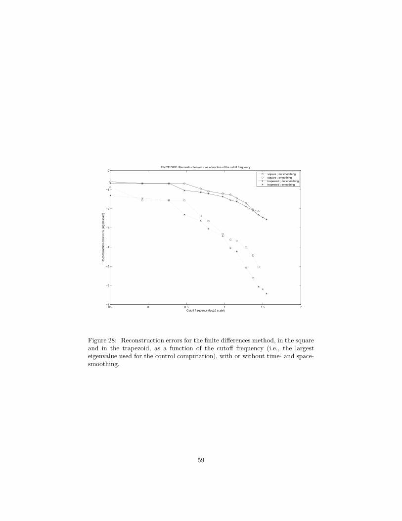
−0.5 0 0.5 1 1.5 2−7
−6
−5
−4
−3
−2
−1
0
Cutoff frequency (log10 scale)
Rec
onst
ruct
ion
erro
r in
% (
log1
0 sc
ale)
FINITE DIFF: Reconstruction error as a function of the cutoff frequency
square ; no smoothingsquare ; smoothingtrapezoid ; no smoothingtrapezoid ; smoothing
Figure 28: Reconstruction errors for the finite differences method, in the squareand in the trapezoid, as a function of the cutoff frequency (i.e., the largesteigenvalue used for the control computation), with or without time- and space-smoothing.
59
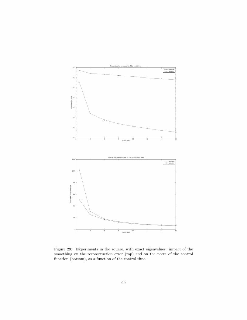
2 4 6 8 10 12 14 1610
−9
10−8
10−7
10−6
10−5
10−4
10−3
10−2
control time
reco
nstr
uctio
n er
ror
Reconstruction error as a fct of the control time
constantsmooth
2 4 6 8 10 12 14 160
200
400
600
800
1000
1200
control time
norm
of t
he c
ontr
ol fu
nctio
n
Norm of the control function as a fct of the control time
constantsmooth
Figure 29: Experiments in the square, with exact eigenvalues: impact of thesmoothing on the reconstruction error (top) and on the norm of the controlfunction (bottom), as a function of the control time.
60
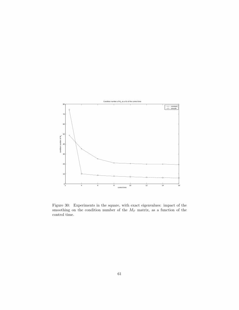
2 4 6 8 10 12 14 160
10
20
30
40
50
60
70
80
control time
cond
ition
num
ber
of M
T
Condition number of MT as a fct of the control time
constantsmooth
Figure 30: Experiments in the square, with exact eigenvalues: impact of thesmoothing on the condition number of the MT matrix, as a function of thecontrol time.
61
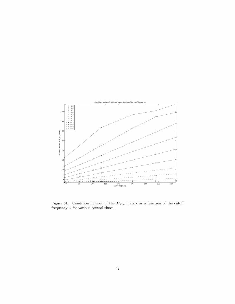
60 80 100 120 140 160 180 200 220
5
10
15
20
25
30
35
40
Cutoff frequency
Con
ditio
n nu
mbe
r of
MT (
log
scal
e)
Condition number of HUM matrix as a function of the cutoff frequency
1.51.61.71.81.922.12.22.32.42.52.6
Figure 31: Condition number of the MT,ω matrix as a function of the cutofffrequency ω for various control times.
62
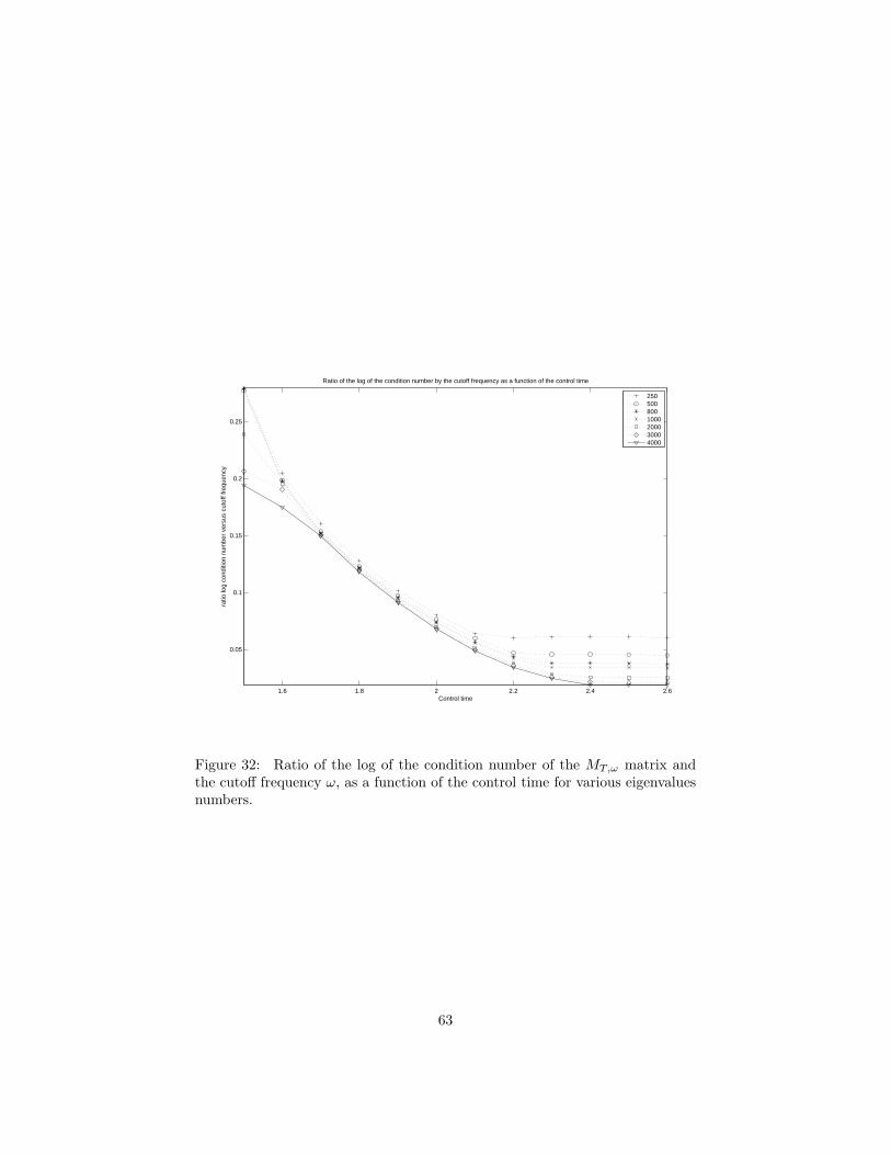
1.6 1.8 2 2.2 2.4 2.6
0.05
0.1
0.15
0.2
0.25
Control time
ratio
log
cond
ition
num
ber
vers
us c
utof
f fre
quen
cy
Ratio of the log of the condition number by the cutoff frequency as a function of the control time
2505008001000200030004000
Figure 32: Ratio of the log of the condition number of the MT,ω matrix andthe cutoff frequency ω, as a function of the control time for various eigenvaluesnumbers.
63
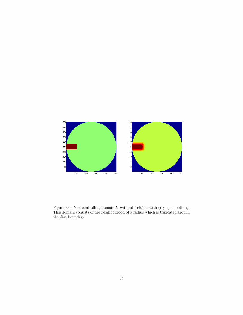
Figure 33: Non-controlling domain U without (left) or with (right) smoothing.This domain consists of the neighborhood of a radius which is truncated aroundthe disc boundary.
64
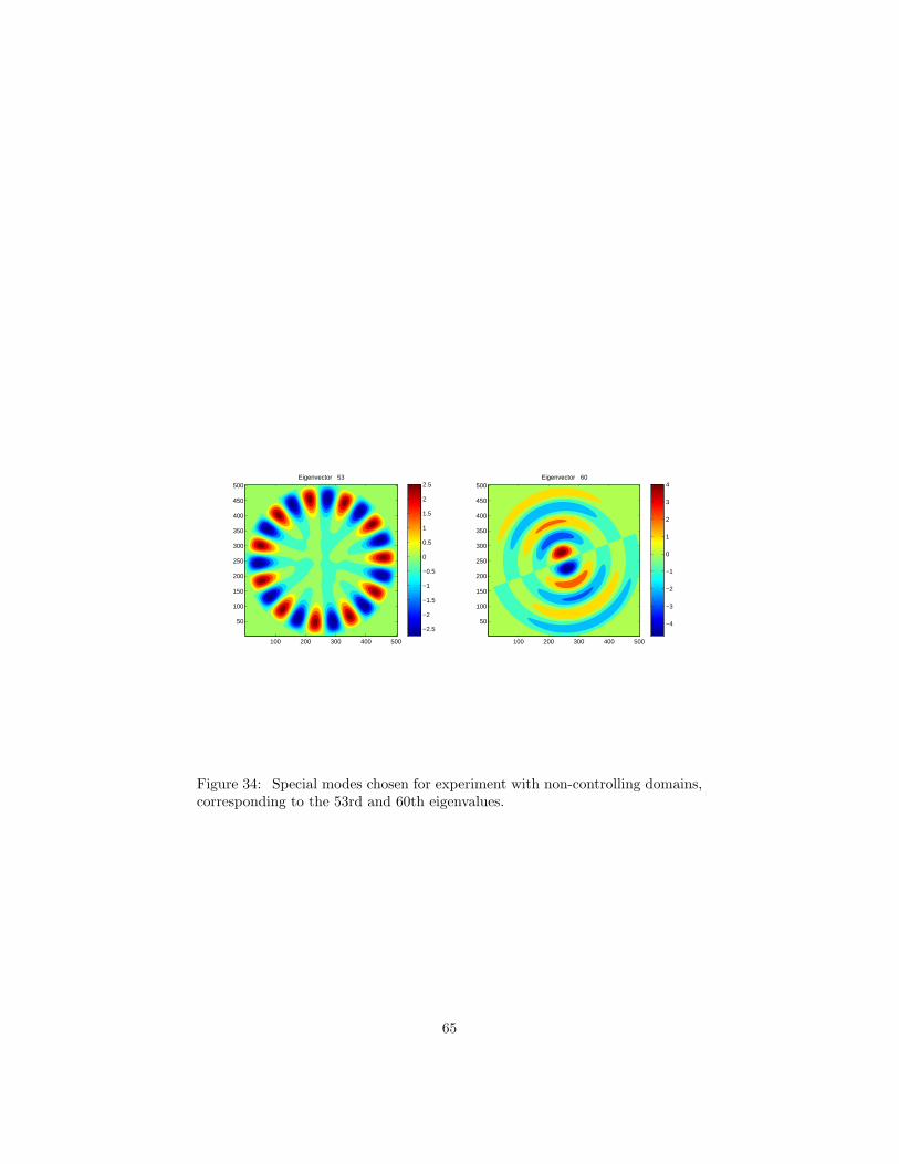
Eigenvector 53
100 200 300 400 500
50
100
150
200
250
300
350
400
450
500
−2.5
−2
−1.5
−1
−0.5
0
0.5
1
1.5
2
2.5Eigenvector 60
100 200 300 400 500
50
100
150
200
250
300
350
400
450
500
−4
−3
−2
−1
0
1
2
3
4
Figure 34: Special modes chosen for experiment with non-controlling domains,corresponding to the 53rd and 60th eigenvalues.
65
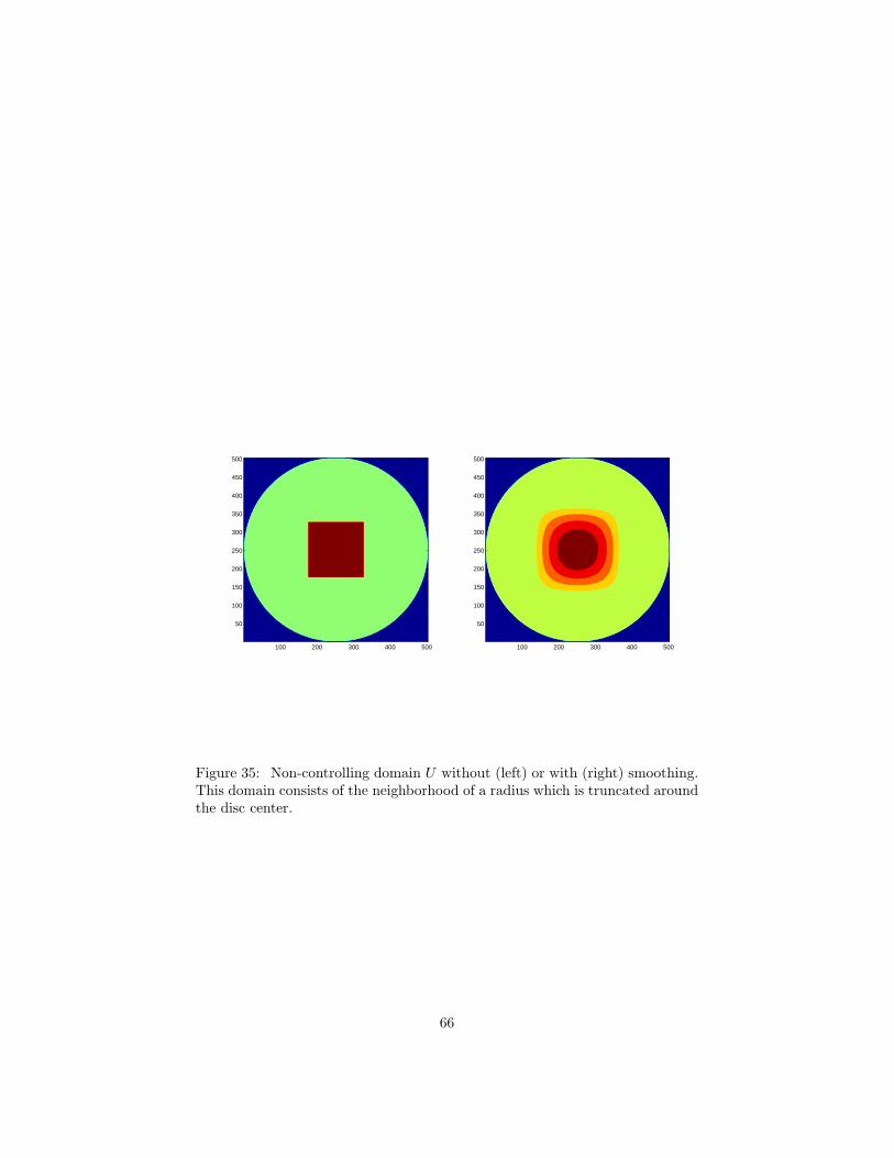
100 200 300 400 500
50
100
150
200
250
300
350
400
450
500
100 200 300 400 500
50
100
150
200
250
300
350
400
450
500
Figure 35: Non-controlling domain U without (left) or with (right) smoothing.This domain consists of the neighborhood of a radius which is truncated aroundthe disc center.
66
List of Tables
1 Validation experiments in the square: Condition num-bers and validation errors for a 100-eigenvalues-experimentin the square (without smoothing), where the eigen-values are exact or computed thanks to finite differences. 68
2 Validation experiments in the square: Condition num-bers and validation errors for various numbers Ne
of eigenvalues used to compute the control function,where the eigenvalues are exact or computed thanksto finite differences. The input data is the 50-th eigen-value, and the reconstruction is performed with 2000eigenvalues. . . . . . . . . . . . . . . . . . . . . . . . 69
3 Impact of the control time, the width of U and thesmoothing, on the condition number of MT , on thereconstruction error and on the norm of the controlfunction. These results come from one-mode experi-ments in the square, with exact eigenvalues. . . . . . 70
4 Influence of the shape of the data on the reconstruc-tion error and the norm of the control, with a non-controlling domain U . On the left, the 53rd eigen-mode is localized around the boundary of the circle,as is the control domain. On the right, the 60th eigen-mode is localized around the center of the circle. . . 71
5 Reconstruction error and the norm of the control witha data u53 localized at the boundary of the disc andtwo different non-controlling domains U , the first onebeing localized around the boundary, the second onearound the center. . . . . . . . . . . . . . . . . . . . 72
67
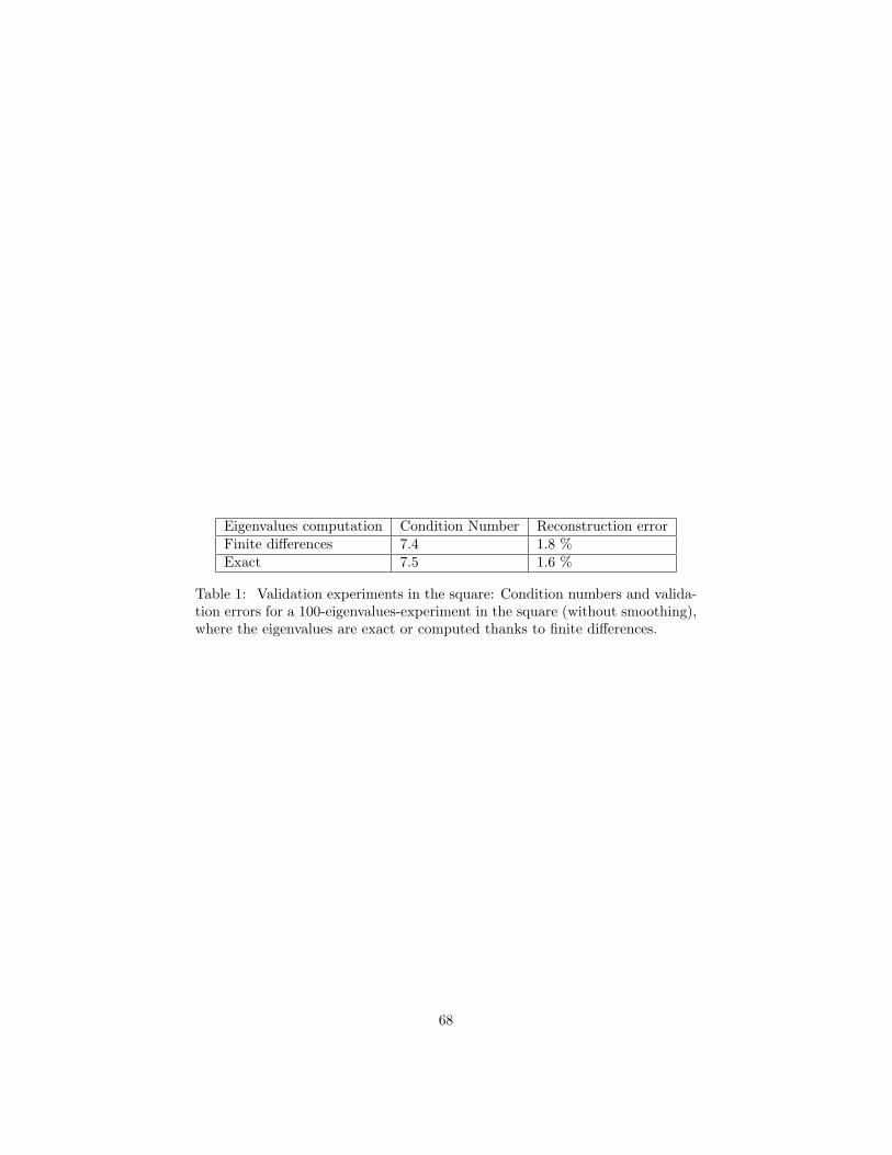
Eigenvalues computation Condition Number Reconstruction errorFinite differences 7.4 1.8 %Exact 7.5 1.6 %
Table 1: Validation experiments in the square: Condition numbers and valida-tion errors for a 100-eigenvalues-experiment in the square (without smoothing),where the eigenvalues are exact or computed thanks to finite differences.
68
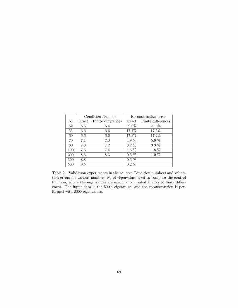
Condition Number Reconstruction errorNe Exact Finite differences Exact Finite differences52 6.5 6.4 29.2% 29.0%55 6.6 6.6 17.7% 17.6%60 6.6 6.6 17.3% 17.2%70 7.1 7.0 4.9 % 5.0 %80 7.3 7.2 3.2 % 3.3 %100 7.5 7.4 1.6 % 1.8 %200 8.3 8.3 0.5 % 1.0 %300 8.8 0.3 %500 9.5 0.2 %
Table 2: Validation experiments in the square: Condition numbers and valida-tion errors for various numbers Ne of eigenvalues used to compute the controlfunction, where the eigenvalues are exact or computed thanks to finite differ-ences. The input data is the 50-th eigenvalue, and the reconstruction is per-formed with 2000 eigenvalues.
69
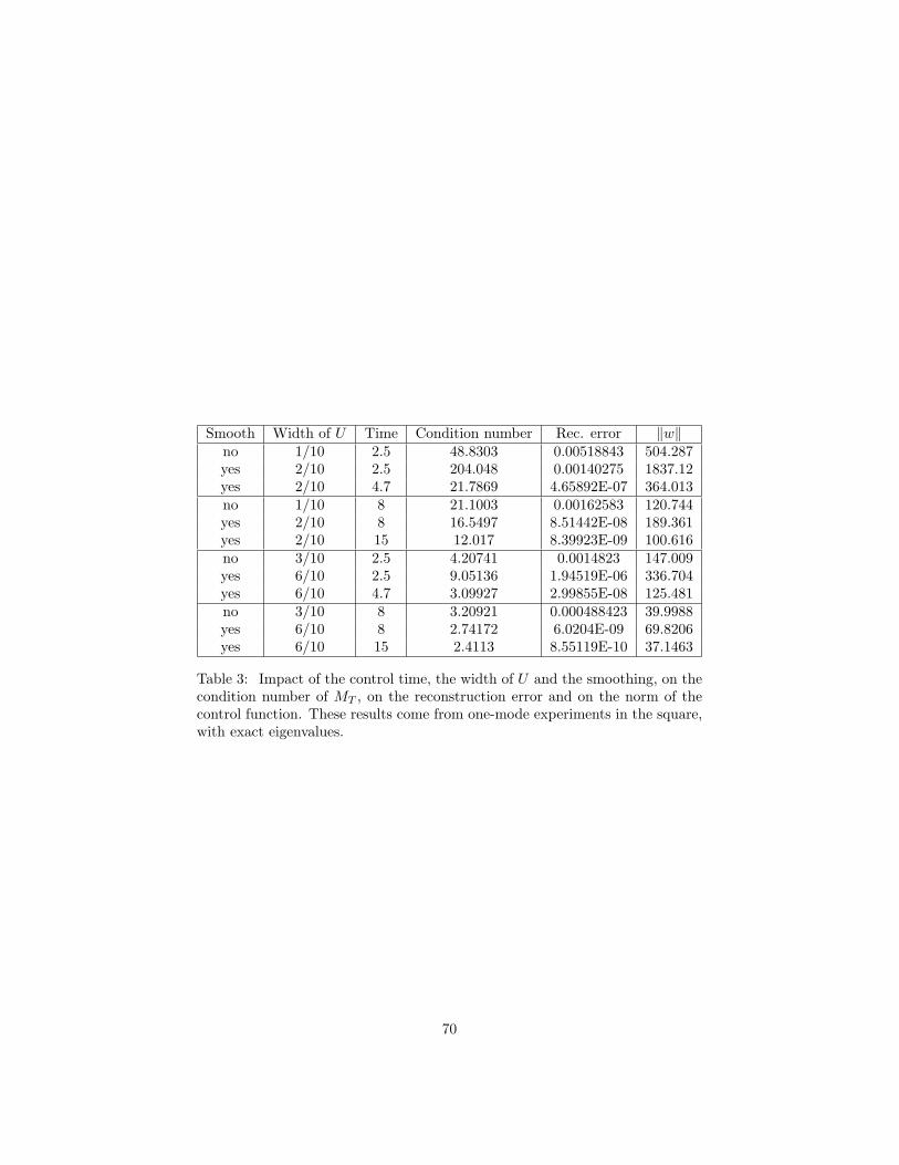
Smooth Width of U Time Condition number Rec. error ‖w‖no 1/10 2.5 48.8303 0.00518843 504.287yes 2/10 2.5 204.048 0.00140275 1837.12yes 2/10 4.7 21.7869 4.65892E-07 364.013no 1/10 8 21.1003 0.00162583 120.744yes 2/10 8 16.5497 8.51442E-08 189.361yes 2/10 15 12.017 8.39923E-09 100.616no 3/10 2.5 4.20741 0.0014823 147.009yes 6/10 2.5 9.05136 1.94519E-06 336.704yes 6/10 4.7 3.09927 2.99855E-08 125.481no 3/10 8 3.20921 0.000488423 39.9988yes 6/10 8 2.74172 6.0204E-09 69.8206yes 6/10 15 2.4113 8.55119E-10 37.1463
Table 3: Impact of the control time, the width of U and the smoothing, on thecondition number of MT , on the reconstruction error and on the norm of thecontrol function. These results come from one-mode experiments in the square,with exact eigenvalues.
70
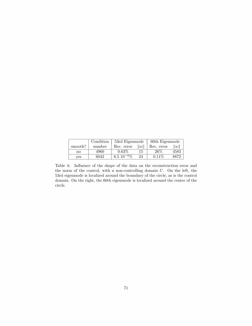
Condition 53rd Eigenmode 60th Eigenmodesmooth? number Rec. error ‖w‖ Rec. error ‖w‖
no 4960 0.63% 15 26% 4583yes 6042 6.5 10−4% 24 0.11% 8872
Table 4: Influence of the shape of the data on the reconstruction error andthe norm of the control, with a non-controlling domain U . On the left, the53rd eigenmode is localized around the boundary of the circle, as is the controldomain. On the right, the 60th eigenmode is localized around the center of thecircle.
71
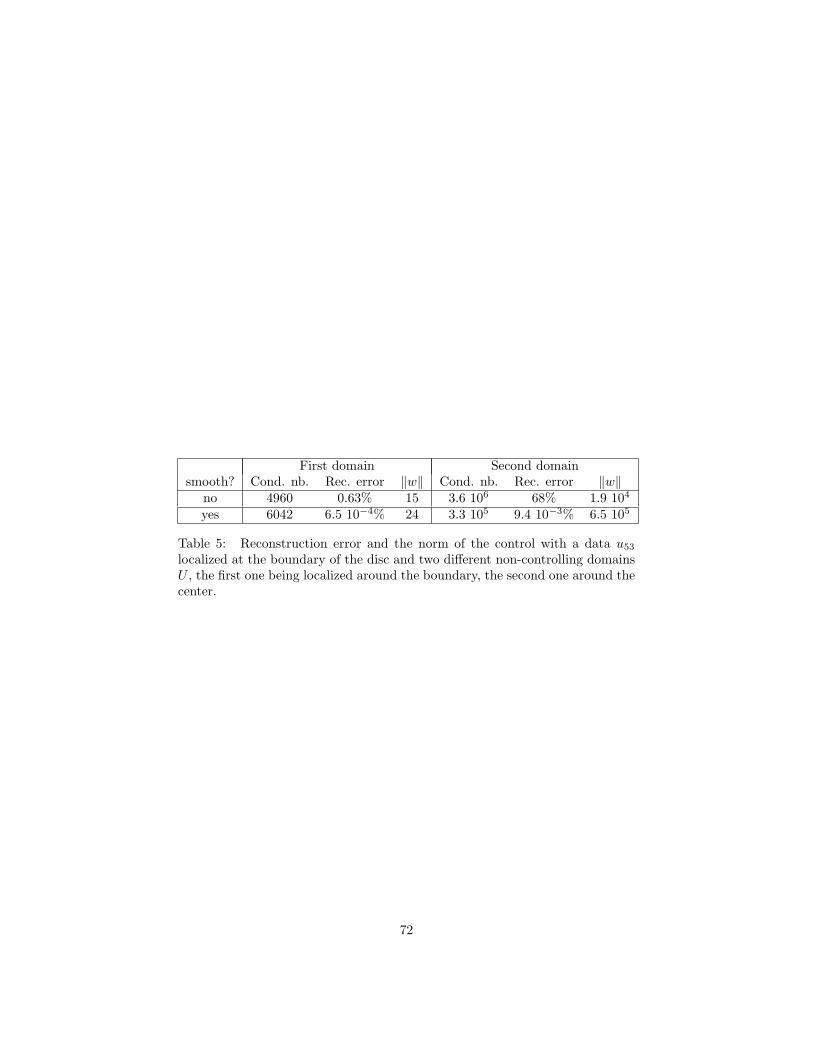
First domain Second domainsmooth? Cond. nb. Rec. error ‖w‖ Cond. nb. Rec. error ‖w‖
no 4960 0.63% 15 3.6 106 68% 1.9 104
yes 6042 6.5 10−4% 24 3.3 105 9.4 10−3% 6.5 105
Table 5: Reconstruction error and the norm of the control with a data u53
localized at the boundary of the disc and two different non-controlling domainsU , the first one being localized around the boundary, the second one around thecenter.
72