arX

iv:0

706.

2741

v1 [

hep-

ex]

19

Jun

2007

EUROPEAN ORGANIZATION FOR NUCLEAR RESEARCH

CERN–PH-EP/2006-008

9 March 2006

Study of Triple-Gauge-BosonCouplings ZZZ, ZZγ and Zγγ at

LEP

DELPHI Collaboration

Abstract

Neutral triple-gauge-boson couplings ZZZ, ZZγ and Zγγ have been stud-ied with the DELPHI detector using data at energies between 183 and208 GeV. Limits are derived on these couplings from an analysis of the re-actions e+e−→ Zγ, using data from the final states γff , with f = q or ν, frome+e−→ ZZ, using data from the four-fermion final states qqqq, qqµ+µ−, qqe+e−,qqνν, µ+µ−νν and e+e−νν, and from e+e−→ Zγ∗, in which the final state γ isoff mass-shell, using data from the four-fermion final states qqe+e− and qqµ+µ−.No evidence for the presence of such couplings is observed, in agreement withthe predictions of the Standard Model.

(Accepted by Euro. Phys. J. C)

ii

J.Abdallah26, P.Abreu23, W.Adam55, P.Adzic12, T.Albrecht18, R.Alemany-Fernandez9, T.Allmendinger18,

P.P.Allport24, U.Amaldi30, N.Amapane48, S.Amato52, E.Anashkin37, A.Andreazza29, S.Andringa23, N.Anjos23,

P.Antilogus26, W-D.Apel18, Y.Arnoud15, S.Ask27, B.Asman47, J.E.Augustin26, A.Augustinus9, P.Baillon9,

A.Ballestrero49 , P.Bambade21, R.Barbier28, D.Bardin17, G.J.Barker57 , A.Baroncelli40 , M.Battaglia9 ,

M.Baubillier26 , K-H.Becks58, M.Begalli7 , A.Behrmann58, E.Ben-Haim21, N.Benekos33, A.Benvenuti5,

C.Berat15 , M.Berggren26 , D.Bertrand2, M.Besancon41 , N.Besson41 , D.Bloch10, M.Blom32 , M.Bluj56,

M.Bonesini30 , M.Boonekamp41, P.S.L.Booth†24, G.Borisov22 , O.Botner53, B.Bouquet21, T.J.V.Bowcock24 ,

I.Boyko17, M.Bracko44, R.Brenner53, E.Brodet36 , P.Bruckman19, J.M.Brunet8, B.Buschbeck55, P.Buschmann58,

M.Calvi30 , T.Camporesi9 , V.Canale39 , F.Carena9, N.Castro23 , F.Cavallo5, M.Chapkin43, Ph.Charpentier9,

P.Checchia37, R.Chierici9, P.Chliapnikov43, J.Chudoba9, S.U.Chung9, K.Cieslik19, P.Collins9 , R.Contri14,

G.Cosme21 , F.Cossutti50 , M.J.Costa54 , D.Crennell38, J.Cuevas35 , J.D’Hondt2, T.da Silva52, W.Da Silva26,

G.Della Ricca50, A.De Angelis51, W.De Boer18, C.De Clercq2, B.De Lotto51, N.De Maria48, A.De Min37,

L.de Paula52, L.Di Ciaccio39 , A.Di Simone40, K.Doroba56, J.Drees58,9, G.Eigen4, T.Ekelof53 , M.Ellert53,

M.Elsing9 , M.C.Espirito Santo23, G.Fanourakis12, D.Fassouliotis12,3 , M.Feindt18, J.Fernandez42, A.Ferrer54,

F.Ferro14, U.Flagmeyer58, H.Foeth9, E.Fokitis33, F.Fulda-Quenzer21, J.Fuster54, M.Gandelman52 , C.Garcia54 ,

Ph.Gavillet9, E.Gazis33 , R.Gokieli9,56 , B.Golob44,46 , G.Gomez-Ceballos42 , P.Goncalves23, E.Graziani40 ,

G.Grosdidier21 , K.Grzelak56, J.Guy38, C.Haag18, A.Hallgren53, K.Hamacher58, K.Hamilton36, S.Haug34,

F.Hauler18, V.Hedberg27, M.Hennecke18, H.Herr†9, J.Hoffman56, S-O.Holmgren47, P.J.Holt9, M.A.Houlden24,

J.N.Jackson24, G.Jarlskog27 , P.Jarry41, D.Jeans36, E.K.Johansson47 , P.Jonsson28, C.Joram9, L.Jungermann18,

F.Kapusta26, S.Katsanevas28, E.Katsoufis33, G.Kernel44, B.P.Kersevan44,46, U.Kerzel18, B.T.King24,

N.J.Kjaer9, P.Kluit32, P.Kokkinias12, C.Kourkoumelis3, O.Kouznetsov17, Z.Krumstein17, M.Kucharczyk19,

J.Lamsa1, G.Leder55, F.Ledroit15, L.Leinonen47, R.Leitner31, J.Lemonne2, V.Lepeltier21, T.Lesiak19,

W.Liebig58, D.Liko55, A.Lipniacka47, J.H.Lopes52, J.M.Lopez35 , D.Loukas12, P.Lutz41, L.Lyons36,

J.MacNaughton55, A.Malek58, S.Maltezos33 , F.Mandl55, J.Marco42 , R.Marco42, B.Marechal52 , M.Margoni37 ,

J-C.Marin9, C.Mariotti9 , A.Markou12, C.Martinez-Rivero42, J.Masik13 , N.Mastroyiannopoulos12 , F.Matorras42 ,

C.Matteuzzi30 , F.Mazzucato37 , M.Mazzucato37 , R.Mc Nulty24, C.Meroni29 , E.Migliore48 , W.Mitaroff55,

U.Mjoernmark27, T.Moa47 , M.Moch18, K.Moenig9,11 , R.Monge14, J.Montenegro32 , D.Moraes52, S.Moreno23,

P.Morettini14, U.Mueller58, K.Muenich58, M.Mulders32, L.Mundim7, W.Murray38, B.Muryn20, G.Myatt36,

T.Myklebust34, M.Nassiakou12, F.Navarria5, K.Nawrocki56, R.Nicolaidou41, M.Nikolenko17,10,

A.Oblakowska-Mucha20, V.Obraztsov43, A.Olshevski17, A.Onofre23, R.Orava16, K.Osterberg16, A.Ouraou41,

A.Oyanguren54, M.Paganoni30 , S.Paiano5, J.P.Palacios24 , H.Palka19, Th.D.Papadopoulou33 , L.Pape9,

C.Parkes25, F.Parodi14 , U.Parzefall9, A.Passeri40 , O.Passon58, L.Peralta23 , V.Perepelitsa54 , A.Perrotta5,

A.Petrolini14, J.Piedra42 , L.Pieri40, F.Pierre41 , M.Pimenta23, E.Piotto9, T.Podobnik44,46 , V.Poireau9,

M.E.Pol6 , G.Polok19 , V.Pozdniakov17, N.Pukhaeva17, A.Pullia30, J.Rames13 , A.Read34, P.Rebecchi9, J.Rehn18,

D.Reid32, R.Reinhardt58, P.Renton36, F.Richard21, J.Ridky13, M.Rivero42, D.Rodriguez42, A.Romero48,

P.Ronchese37, P.Roudeau21, T.Rovelli5, V.Ruhlmann-Kleider41, D.Ryabtchikov43, A.Sadovsky17, L.Salmi16,

J.Salt54, C.Sander18, A.Savoy-Navarro26, U.Schwickerath9, R.Sekulin38, M.Siebel58, A.Sisakian17, G.Smadja28,

O.Smirnova27, A.Sokolov43, A.Sopczak22, R.Sosnowski56, T.Spassov9, M.Stanitzki18, A.Stocchi21, J.Strauss55,

B.Stugu4, M.Szczekowski56, M.Szeptycka56, T.Szumlak20, T.Tabarelli30 , F.Tegenfeldt53, J.Timmermans32 ,

L.Tkatchev17, M.Tobin24, S.Todorovova13, B.Tome23, A.Tonazzo30, P.Tortosa54 , P.Travnicek13, D.Treille9,

G.Tristram8, M.Trochimczuk56, C.Troncon29, M-L.Turluer41, I.A.Tyapkin17, P.Tyapkin17, S.Tzamarias12 ,

V.Uvarov43, G.Valenti5, P.Van Dam32, J.Van Eldik9, N.van Remortel16, I.Van Vulpen9, G.Vegni29, F.Veloso23,

W.Venus38, P.Verdier28, V.Verzi39, D.Vilanova41, L.Vitale50, V.Vrba13, H.Wahlen58, A.J.Washbrook24,

C.Weiser18, D.Wicke9, J.Wickens2, G.Wilkinson36, M.Winter10, M.Witek19, O.Yushchenko43, A.Zalewska19,

P.Zalewski56 , D.Zavrtanik45, V.Zhuravlov17, N.I.Zimin17, A.Zintchenko17, M.Zupan12

iii

1Department of Physics and Astronomy, Iowa State University, Ames IA 50011-3160, USA2IIHE, ULB-VUB, Pleinlaan 2, B-1050 Brussels, Belgium3Physics Laboratory, University of Athens, Solonos Str. 104, GR-10680 Athens, Greece4Department of Physics, University of Bergen, Allegaten 55, NO-5007 Bergen, Norway5Dipartimento di Fisica, Universita di Bologna and INFN, Via Irnerio 46, IT-40126 Bologna, Italy6Centro Brasileiro de Pesquisas Fısicas, rua Xavier Sigaud 150, BR-22290 Rio de Janeiro, Brazil7Inst. de Fısica, Univ. Estadual do Rio de Janeiro, rua Sao Francisco Xavier 524, Rio de Janeiro, Brazil8College de France, Lab. de Physique Corpusculaire, IN2P3-CNRS, FR-75231 Paris Cedex 05, France9CERN, CH-1211 Geneva 23, Switzerland

10Institut de Recherches Subatomiques, IN2P3 - CNRS/ULP - BP20, FR-67037 Strasbourg Cedex, France11Now at DESY-Zeuthen, Platanenallee 6, D-15735 Zeuthen, Germany12Institute of Nuclear Physics, N.C.S.R. Demokritos, P.O. Box 60228, GR-15310 Athens, Greece13FZU, Inst. of Phys. of the C.A.S. High Energy Physics Division, Na Slovance 2, CZ-182 21, Praha 8, Czech Republic14Dipartimento di Fisica, Universita di Genova and INFN, Via Dodecaneso 33, IT-16146 Genova, Italy15Institut des Sciences Nucleaires, IN2P3-CNRS, Universite de Grenoble 1, FR-38026 Grenoble Cedex, France16Helsinki Institute of Physics and Department of Physical Sciences, P.O. Box 64, FIN-00014 University of Helsinki,Finland

17Joint Institute for Nuclear Research, Dubna, Head Post Office, P.O. Box 79, RU-101 000 Moscow, Russian Federation18Institut fur Experimentelle Kernphysik, Universitat Karlsruhe, Postfach 6980, DE-76128 Karlsruhe, Germany19Institute of Nuclear Physics PAN,Ul. Radzikowskiego 152, PL-31142 Krakow, Poland20Faculty of Physics and Nuclear Techniques, University of Mining and Metallurgy, PL-30055 Krakow, Poland21Universite de Paris-Sud, Lab. de l’Accelerateur Lineaire, IN2P3-CNRS, Bat. 200, FR-91405 Orsay Cedex, France22School of Physics and Chemistry, University of Lancaster, Lancaster LA1 4YB, UK23LIP, IST, FCUL - Av. Elias Garcia, 14-1o, PT-1000 Lisboa Codex, Portugal24Department of Physics, University of Liverpool, P.O. Box 147, Liverpool L69 3BX, UK25Dept. of Physics and Astronomy, Kelvin Building, University of Glasgow, Glasgow G12 8QQ26LPNHE, IN2P3-CNRS, Univ. Paris VI et VII, Tour 33 (RdC), 4 place Jussieu, FR-75252 Paris Cedex 05, France27Department of Physics, University of Lund, Solvegatan 14, SE-223 63 Lund, Sweden28Universite Claude Bernard de Lyon, IPNL, IN2P3-CNRS, FR-69622 Villeurbanne Cedex, France29Dipartimento di Fisica, Universita di Milano and INFN-MILANO, Via Celoria 16, IT-20133 Milan, Italy30Dipartimento di Fisica, Univ. di Milano-Bicocca and INFN-MILANO, Piazza della Scienza 3, IT-20126 Milan, Italy31IPNP of MFF, Charles Univ., Areal MFF, V Holesovickach 2, CZ-180 00, Praha 8, Czech Republic32NIKHEF, Postbus 41882, NL-1009 DB Amsterdam, The Netherlands33National Technical University, Physics Department, Zografou Campus, GR-15773 Athens, Greece34Physics Department, University of Oslo, Blindern, NO-0316 Oslo, Norway35Dpto. Fisica, Univ. Oviedo, Avda. Calvo Sotelo s/n, ES-33007 Oviedo, Spain36Department of Physics, University of Oxford, Keble Road, Oxford OX1 3RH, UK37Dipartimento di Fisica, Universita di Padova and INFN, Via Marzolo 8, IT-35131 Padua, Italy38Rutherford Appleton Laboratory, Chilton, Didcot OX11 OQX, UK39Dipartimento di Fisica, Universita di Roma II and INFN, Tor Vergata, IT-00173 Rome, Italy40Dipartimento di Fisica, Universita di Roma III and INFN, Via della Vasca Navale 84, IT-00146 Rome, Italy41DAPNIA/Service de Physique des Particules, CEA-Saclay, FR-91191 Gif-sur-Yvette Cedex, France42Instituto de Fisica de Cantabria (CSIC-UC), Avda. los Castros s/n, ES-39006 Santander, Spain43Inst. for High Energy Physics, Serpukov P.O. Box 35, Protvino, (Moscow Region), Russian Federation44J. Stefan Institute, Jamova 39, SI-1000 Ljubljana, Slovenia45Laboratory for Astroparticle Physics, University of Nova Gorica, Kostanjeviska 16a, SI-5000 Nova Gorica, Slovenia46Department of Physics, University of Ljubljana, SI-1000 Ljubljana, Slovenia47Fysikum, Stockholm University, Box 6730, SE-113 85 Stockholm, Sweden48Dipartimento di Fisica Sperimentale, Universita di Torino and INFN, Via P. Giuria 1, IT-10125 Turin, Italy49INFN,Sezione di Torino and Dipartimento di Fisica Teorica, Universita di Torino, Via Giuria 1, IT-10125 Turin, Italy50Dipartimento di Fisica, Universita di Trieste and INFN, Via A. Valerio 2, IT-34127 Trieste, Italy51Istituto di Fisica, Universita di Udine and INFN, IT-33100 Udine, Italy52Univ. Federal do Rio de Janeiro, C.P. 68528 Cidade Univ., Ilha do Fundao BR-21945-970 Rio de Janeiro, Brazil53Department of Radiation Sciences, University of Uppsala, P.O. Box 535, SE-751 21 Uppsala, Sweden54IFIC, Valencia-CSIC, and D.F.A.M.N., U. de Valencia, Avda. Dr. Moliner 50, ES-46100 Burjassot (Valencia), Spain55Institut fur Hochenergiephysik, Osterr. Akad. d. Wissensch., Nikolsdorfergasse 18, AT-1050 Vienna, Austria56Inst. Nuclear Studies and University of Warsaw, Ul. Hoza 69, PL-00681 Warsaw, Poland57Now at University of Warwick, Coventry CV4 7AL, UK58Fachbereich Physik, University of Wuppertal, Postfach 100 127, DE-42097 Wuppertal, Germany

† deceased

1

1 Introduction

One of the important properties of the Standard Model which can be tested at LEP2is its non-Abelian character, leading to the prediction of triple-gauge-boson couplings.However, while non-zero values of these couplings are predicted for the charged (WWγ,WWZ) sector, the SU(2)× U(1) symmetry of the Standard Model predicts the absenceof such couplings in the neutral sector, namely at the ZZZ, ZZγ and Zγγ vertices. Thispaper describes an investigation of this prediction by DELPHI using LEP2 data takenbetween 1997 and 2000 at energies between 183 and 208 GeV.

1.1 Phenomenology of the neutral triple-gauge-boson vertex

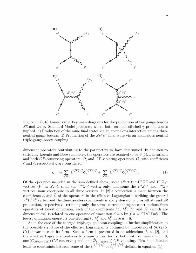
Within the Standard Model, production of two neutral gauge bosons in e+e− collisionsproceeds at lowest order via the t- or u-channel exchange of an electron. These processesare shown in figures 1a) and b), where both on- and off-shell γ production is implied, asis the subsequent decay of the final state Z or off-shell γ into a fermion-antifermion pair.Figure 1c) shows a contribution to production of the same final states which could comefrom physics beyond the Standard Model by the s-channel exchange of a virtual γ or Zvia a neutral triple-gauge-boson coupling. In the reactions e+e−→ Zγ and e+e−→ ZZthe final state can, to a good approximation, be considered to be of two on-shell bosons,so that only the exchanged boson at the triple-gauge-boson vertex need necessarily beconsidered as off-shell, while in the reaction e+e−→ Zγ∗ both the exchanged boson andthe outgoing γ∗ are off-shell.1 A further process containing a neutral triple-gauge-bosoncoupling with two of the bosons off-shell is shown in figure 1d); here a single Z is producedin the final state Ze+e− via fusion of two exchanged vector bosons.

The phenomenology of the case where two of the three neutral gauge bosons inter-acting at the V 0

1 V02 V

03 vertex are on mass-shell has been described in [1]. In this case,

there are twelve independent anomalous couplings satisfying Lorentz invariance and Bosesymmetry. Calling V the exchanged boson (V = Z, γ), the couplings fV

i (i =4,5) producea ZZ final state and hV

i (i = 1 · · ·4) the Zγ final state. The couplings fV5 , hV

3 and hV4 are

CP-conserving and fV4 , hV

1 and hV2 are CP-violating. There are no couplings common to

production of both the ZZ and Zγ final states.A complete phenomenological description of the anomalous neutral gauge couplings in

the case where one, two or three of the gauge bosons interacting at the V 01 V

02 V

03 vertex

may be off mass-shell has been developed in [2]. Following the treatment of the chargedtriple-gauge-boson vertex developed, for instance, in [3,4], all the Lorentz-invariant formswhich can contribute to the ZZZ, ZZγ and Zγγ vertices are listed, imposing Bosesymmetry as appropriate. An effective Lagrangian model is then developed in terms ofthe operators of lowest dimension which are required to reconstruct fully all the vertexforms, and which affect only the neutral triple-gauge-boson vertex.2 This leads to aLagrangian with operators of dimension, d, ranging from d = 6 to d = 12. Such anexpansion is valid in the case where the new physics energy scale, Λ, represented by theoperators is very high, at least satisfying the condition Λ ≫ (mZ ,

√s), and the relative

contribution from an operator of dimension d may be expected to be suppressed bya factor 1/Λ(d−4). In the analysis we report here, we have considered only the lowest

1Throughout this paper, we write “V ∗” when we wish to be explicit that a vector boson V is off mass-shell. When it isclear that it is on mass-shell, or when it can be either on or off mass-shell, the star (“∗”) is omitted.

2The V 01V 02V 03

vertex functions receive contributions from both transverse and scalar terms, the latter contributing inthe case where one off-shell Z decays to a heavy fermion pair through its axial coupling. In the analysis of LEP data onlytransverse terms need be considered, due to the negligible contribution of Z →tt decays. The contribution of scalar termsis therefore ignored in the following.

2

a)e+

e−

Z/γ

Z

b)e+

e−

Z/γ

Z

c)e+

e−

Z/γ

Z

Z∗/γ∗

d)e+

e−

e+

e−

Z

Z∗/γ∗

Z∗/γ∗

Figure 1: a), b) Lowest order Feynman diagrams for the production of two gauge bosonsZZ and Zγ by Standard Model processes, where both on- and off-shell γ production isimplied. c) Production of the same final states via an anomalous interaction among threeneutral gauge bosons. d) Production of the Ze+e− final state via an anomalous neutraltriple-gauge-boson coupling.

dimension operators contributing to the parameters we have determined. In addition tosatisfying Lorentz and Bose symmetry, the operators are required to be U(1)em-invariant,and both CP -conserving operators, O, and CP -violating operators, O, with coefficientsℓ and ℓ, respectively, are considered:

L = e(∑

i,CP+

ℓV 01V 02V 03

i OV 01V 02V 03

i +∑

i,CP−

ℓV 01V 02V 03

i OV 01V 02V 03

i ) . (1)

Of the operators included in the sum defined above, some affect the V 0ZZ and V 0Zγ∗

vertices (V 0 ≡ Z, γ), some the V 0Zγ∗ vertex only, and some the V 0Zγ∗ and V 0Zγvertices; none contribute to all three vertices. In [2] a connection is made between the

coefficients ℓi and ℓi of the operators in the effective Lagrangian describing the generalV 01 V

02 V

03 vertex and the dimensionless coefficients h and f describing on-shell Zγ and ZZ

production, respectively: retaining only the terms corresponding to contributions fromoperators of lowest dimension, each of the coefficients hV

1 , hV3 , f

V4 and fV

5 (which are

dimensionless) is related to one operator of dimension d = 6 by f, h = ℓV01V 02V 03 m2

Z . Thelowest dimension operators contributing to hV

2 and hV4 have d = 8.

As in the case of the charged triple-gauge-boson couplings, a further simplification inthe possible structure of the effective Lagrangian is obtained by imposition of SU(2) ×U(1) invariance on its form. Such a form is presented in an addendum [5] to [2], andthe effective Lagrangian reduces to a sum of two terms, both with dimension d = 8,one (OSU(2)×U(1)) CP -conserving and one (OSU(2)×U(1)) CP -violating. This simplification

leads to constraints between some of the ℓV 01V 02V 03

i or ℓV 01V 02V 03

i defined in equation (1):

3

ℓ ZZZ1 cot θW = ℓ ZZγ

1 = −ℓ ZZγ2 = −ℓ Zγγ

1 tan θW =v2

4ℓSU(2)×U(1) , (2)

ℓ ZZZ1 cot θW = ℓ ZZγ

1 = −ℓ ZZγ3 = −ℓ Zγγ

1 tan θW =v2

4ℓSU(2)×U(1) , (3)

where θW is the weak mixing angle, v is the vacuum expectation value of the Higgsfield and ℓSU(2)×U(1), ℓSU(2)×U(1) are the coefficients of the operators OSU(2)×U(1) and

OSU(2)×U(1), respectively. If applied solely to the on-shell channels Zγ and ZZ, theseconditions become, respectively:

fZ5 cot θW = hZ

3 = −f γ5 = −hγ

3 tan θW = m2Z

v2

4ℓSU(2)×U(1) , (4)

fZ4 cot θW = hZ

1 = −f γ4 = −hγ

1 tan θW = m2Z

v2

4ℓSU(2)×U(1) . (5)

The SU(2)× U(1)-conserving Lagrangian considered in [2] is constructed so as to affectonly the neutral gauge boson and Higgs sectors, and an alternative form, which wouldadditionally affect off-mass-shell charged gauge boson production, has been proposedin [6]. This leads to a Lagrangian with four possible terms, two CP -conserving (OA

8 , OB8 )

and two CP -violating (OA8 , OB

8 ) and hence to looser constraints between the possiblecontributing operators: in each of the sets of conditions (2) - (5) listed above, the relationscorresponding in the diagrams of figure 1 to γ and Z exchange decouple, giving, forinstance in the case of (2), the separate conditions

ℓ ZZZ1 cot θW = ℓ ZZγ

1 and ℓ ZZγ2 = ℓ Zγγ

1 tan θW , (6)

with an analogous separation in conditions (3) - (5). This leads to four coefficients, ℓA,B8 ,

ℓA,B8 , related to the respective Lagrangian operators by appropriate factors of mZ andv. In both the stronger and weaker of these sets of constraints (which we refer to asthe Gounaris-Layssac-Renard and Alcaraz constraints, with respect to the authorshipof references [2] and [6]), the gauge-invariant operators all now contribute to all threeneutral triple-gauge-boson vertices, V 0ZZ, V 0Zγ∗ and V 0Zγ.

In order to study the V 01 V

02 V

03 vertex, three physical final states have been defined

from the data: Zγ, Zγ∗ and ZZ. The first of these is a three-body final state comprisingthe Z decay products and a detected photon, while the other two are four-fermion finalstates with, respectively, one or two fermion-antifermion pairs having mass in the Zregion. Given the phenomenology summarized above, we have then chosen to determinethe following parameters in our study:

• Using data from the final states ZZ and Zγ∗, values are determined for the coefficientsof each of the four d = 6 operators which are related in the on-shell limit to oneof the f coefficients defined in the on-shell formalism of reference [1]. Similarly,using data from the final states Zγ, Zγ∗ and ZZ, values of the coefficients of the fourd = 6 operators related to the on-shell h coefficients are determined. In the lattercase, the ZZ data are used as well as the Zγ∗, as the off-shell γ couples to the f fsystem over the whole of the four-fermion phase space. However, in these studies thestatistical contribution of the off-shell final states compared to that of on-shell Zγ orZZ production is very small, so that the values of the parameters determined, quotedin dimensionless form, ℓV

01V 02V 03 m2

Z , are directly comparable with published resultsusing data from on-shell channels, and the relevant respective likelihood distributionsmay be combined.

4

• The V 0Zγ∗ vertex is studied on its own by determining the coefficients of the lowestdimension operators which affect solely these vertices. There are two such operators,both of dimension d = 8, one CP -conserving and involving s-channel γ exchangein the production process illustrated in figure 1c), and the other CP -violating andinvolving s-channel Z exchange in the same diagram. Again, data from both theZγ∗ and ZZ final states were used in the determination of the coefficients of theseoperators, and the coefficients are quoted in dimensionless form: ℓV

01V 02V 03 m4

Z .• The coefficients of the SU(2) × U(1)-conserving operators are determined, usingboth the Gounaris-Layssac-Renard and the Alcaraz constraints. They are quoted ina dimensionless form, such that in the on-shell limit they become equal to one ofthe hV

i occurring in the constraint equations (4) and (5) above.

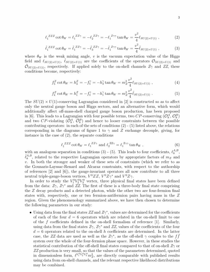
A list of the parameters we have determined, the definitions of the operators to whichthey refer and (where relevant) the on-shell coefficients to which they are related is givenin table 1.

1.2 Experimental considerations

Of the three final state channels, Zγ, ZZ and Zγ∗, defined in the previous section,the most precise limits on anomalous couplings are derived from the first, when thefinal state photon is on-shell. In this channel, the kinematic region with high photonenergy and large photon polar angle is most sensitive to the anomalous couplings, and inthis region the anomalous interactions give rise to a change in the total rate and to anenhancement of the production of longitudinally polarized Z bosons. Our analysis coverstwo reactions to which the diagrams describing Zγ production provide the dominantcontribution: e+e− → ννγ, in which the observed number of events is compared withthe number predicted from the total cross-section for this process, and e+e− → qqγ, withthe qq system coming predominantly from Z decay, in which the distribution of the decayangle of the Z in its rest frame with respect to the direction of the Z in the overall centreof mass is studied. The present analysis uses data from LEP2 at energies ranging from189 to 208 GeV. Previous DELPHI results on this channel can be found in [7]; they useddata with energies up to

√s = 172 GeV, and the limits were obtained using an analysis

based only on the value of the observed total cross-section.The total ZZ cross-section is also sensitive to the anomalous couplings, and the sen-

sitivity increases strongly with√s. Large interference between Standard Model and

anomalous amplitudes arises for CP -conserving couplings (especially for fZ5 ) when con-

sidering the differential cross-section dσ/d| cos θZ |, where θZ is the Z production anglewith respect to the beam axis. The analysis reported here is based on a study of thisdifferential distribution in the LEP2 data in the energy range 183 to 208 GeV. DELPHIhas previously reported a study of the ZZ production cross-section in all visible f1f2f3f4final states in these data [8]. The same sets of identified events have been used in thepresent analysis, with the exception of the qqτ+τ−, τ+τ−νν and l+l−l+l− channels, whichare not used.

In a separate publication [9], DELPHI has studied the Zγ∗ final state in the sameLEP2 data as used for the channels described above, reporting on a comparison of thecross-section for Zγ∗ production in various channels with Standard Model predictions.We use the samples identified in [9] in the qqe+e− and qqµ+µ− final states in the presentanalysis, which thus represents an interpretation of these data for the first time in termsof possible anomalous gauge couplings. The data were examined as a function of thebidimensional (Ml+l−, Mqq) mass distribution, requiring one of them to be in the region

5

Vertices Parameter Lagrangian Related on-shellaffected Operator coefficient

a)

ZZZ ℓ ZZZ1 m2

Z −Zσ(∂σZν)(∂µZ

µν) fZ4

ℓ ZZZ1 m2

Z Zµν(∂σZσµ)Zν fZ

5

ZZγ ℓ ZZγ3 m2

Z −(∂µFµβ)Zα(∂

αZβ) f γ4

ℓ ZZγ2 m2

Z ZµνZν(∂σFσµ) f γ

5

ℓ ZZγ1 m2

Z −F µβZβ(∂σZσµ) hZ

1

ℓ ZZγ1 m2

Z −FµνZν(∂σZ

σµ) hZ3

Zγγ ℓ Zγγ1 m2

Z −(∂σFσµ)ZβFµβ hγ

1

ℓ Zγγ1 m2

Z −Fρα(∂σFσρ)Zα hγ

3

b)

ZZγ ℓ ZZγ4 m4

Z ∂µFµν(✷∂νZα)Z

α –

Zγγ ℓ Zγγ2 m4

Z ✷F µν(∂σFσµ)Zν –

c) i)

ZZZ ZZγ Zγγ − cot θWm2Z

v2

4ℓSU(2)×U(1) iBµν(∂σB

σµ)(Φ†DνΦ) hγ1

− cot θWm2Z

v2

4ℓSU(2)×U(1) iBµν(∂σB

σµ)(Φ†DνΦ) hγ3

ii)

ZZγ − cot θWm2Z

v2

4ℓA8 iBµν(∂σB

σµ)(Φ†DνΦ) hγ1

− cot θWm2Z

v2

4ℓA8 iBµν(∂σB

σµ)(Φ†DνΦ) hγ3

ZZZ Zγγ − cot θWm2Z

v2

4ℓB8 iBµν(∂σW

σµI )(Φ†τID

νΦ) hZ1

− cot θWm2Z

v2

4ℓB8 iBµν(∂σW

σµI )(Φ†τID

νΦ) hZ3

Table 1: Parameters determined in this study, corresponding Lagrangian operators inthe models of references [2] and [6], and (where appropriate) related on-shell parameters:a) Coefficients of lowest dimension operators contributing to ZZ and Zγ∗ production or toZγ∗ and Zγ production; b) Coefficients of lowest dimension operators affecting only theV 0Zγ∗ vertices; c) Coefficients of SU(2)× U(1)-conserving operators according to i) theGounaris-Layssac-Renard constraints and ii) the Alcaraz constraints. The constraints aregiven in the text. The vertices V 0

1 V02 V

03 affected by these operators (without distinguish-

ing the V 0i as on- or off-mass-shell) are indicated in column 1. The fields Zµ, Fµ, Bµ and

Wµ represent the Z, photon, U(1)Y and SU(2)L fields, respectively; Zµν , Fµν and Bµν arethe contractions of the respective field tensors with the four-dimensional antisymmetrictensor; Φ is the Higgs field and v its vacuum expectation value, D represents the covariantderivative of SU(2)× U(1), and τI are the Pauli matrices.

6

of the Z mass, and they were also divided into two regions of the l+l− polar angle withrespect to the beam direction (equivalent to the variable θZ used in the analysis of ZZevents).

Limits on anomalous neutral gauge couplings in the Zγ and ZZ final states have beenreported by other LEP experiments; recent published results may be found in the paperslisted in [10,11].

2 Experimental details and analysis

Events were recorded in the DELPHI detector. Detailed descriptions of the DELPHIcomponents can be found in [12] and the description of its performance and of the lumi-nosity monitor can be found in [13]. The trigger system is described in [14]. For LEP2operations, the vertex detector was upgraded [15], and a set of scintillation counters wasadded to veto photons in the blind regions of the electromagnetic calorimetry at polar an-gles around θ = 40◦. The performance of the detector was simulated using the programDELSIM [13], which was interfaced to the programs used in the generation of MonteCarlo events and to the programs used to simulate the hadronization of quarks from Zand γ∗ decay or from background processes. During the year 2000, one sector (1/12) ofthe Time Projection Chamber (TPC), DELPHI’s main tracking device, was inactive forabout a quarter of the data-taking period. The effect of this was taken into account inthe detector simulation and in the determination of cross-sections from the data.

The selection of events in the three physical final states, Zγ, ZZ and Zγ∗, considered inthis paper, and the simulation of the processes contributing to signals and backgroundsare described in the following subsections. In the case of the ZZ and Zγ∗ samples, thereader is referred to recent DELPHI publications on the production of these final states(references [8,9], respectively) for a full description of the event selection procedures. Theevent samples used in the present analysis of these two final states have been selectedusing essentially identical procedures to those described in [8,9], and cover the same energyrange (183 - 208 GeV). These procedures are summarized, respectively, in sections 2.2and 2.3 below, and any changes from the methods described in [8,9] are mentioned.DELPHI has also reported a study of events observed at LEP2 in which only photonsand missing energy were detected [16]. The present analysis uses data in the part of thekinematic region covered in [16] in which a high energy photon is produced at a largeangle with respect to the beam direction; data in the energy range 189 - 208 GeV havebeen used. The selection procedures specific to this final state as well as to that in which aquark-antiquark pair is produced, rather than missing energy, are described in section 2.1below.

In the final year of LEP running, data were taken over a range of energies from 205 to208 GeV. The values of the centre-of-mass energy quoted in the descriptions below forthat year correspond to the averages for the data samples collected.

2.1 The Zγ final state

The selection procedure for Zγ production in the kinematic region with greatest sen-sitivity to anomalous gauge couplings concentrated on a search for events with a veryenergetic photon in the angular range 45◦ < θγ < 135◦, where θγ is the polar angle of thephoton with respect to the beam direction. This angular region is covered by DELPHI’sbarrel electromagnetic calorimeter, the High density Projection Chamber (HPC). Thesearch was conducted in events with two final state topologies: ννγ and qqγ.

7

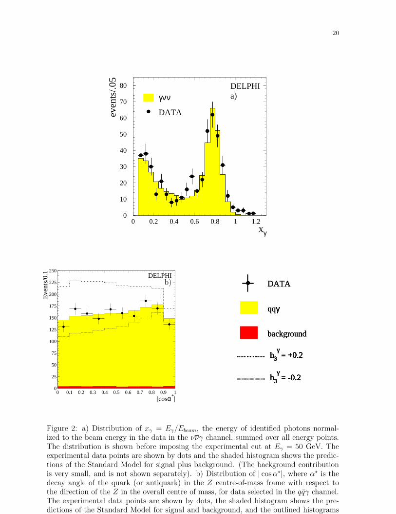
The ννγ sample was selected from events with a detected final state containing only asingle photon. Its energy, Eγ , was required to be greater than 50 GeV and only photonsin the range covered by the HPC, 45◦ < θγ < 135◦ were accepted. No tracks or hits wereallowed in the TPC. It was also required that no electromagnetic showers with energyexceeding defined background noise levels were present in the forward electromagneticcalorimeter and the luminosity monitor. Further showers in the HPC were accepted onlyif they were within 20◦ of the first one, and such showers were then combined. Cosmicray events were suppressed by requiring that any signal in the hadronic calorimeter bein the same angular region as the signal in the electromagnetic calorimeter, and that theelectromagnetic shower point towards the beam collision point within an angle of 15◦.The trigger efficiency was measured using Compton and Bhabha events. The expectednumbers of events were calculated using the generators NUNUGPV, based on [17], andKORALZ [18], interfaced to the full DELPHI simulation program. The results obtainedapplying these criteria are shown in table 2. From the simulations, the efficiency fordetecting ννγ events in the kinematic region considered here was shown to be independentof the centre-of-mass energy, with an average value of (50.7 ± 2.0)% for the data samplelisted in table 2. Contributions from background sources to this channel were estimatedto be negligible. Full details of the analysis of this final state may be found in [16].The distribution of xγ , the energy of identified photons normalized to the beam energy(xγ = Eγ/Ebeam) before imposing the cut at Eγ = 50 GeV is shown for photons withxγ > 0.05 in figure 2a), which also shows the expectation of the Standard Model.

√s Integrated Selected Total predicted

(GeV) luminosity (pb−1) data events188.6 154.7 87 89.2191.6 25.1 14 13.1195.5 76.2 32 37.5199.5 83.1 45 38.5201.6 40.6 20 18.2206.1 214.6 98 102.3

Total 594.3 296 298.8

Table 2: ννγ final state: Integrated luminosity and numbers of observed and expectedevents at each energy,

√s.

In the selection of events in the qqγ channel, the same requirements were imposedon the energy and polar angle of photon candidates as in the ννγ case, namely: Eγ >50 GeV and 45◦ < θγ < 135◦. In addition, events were required to have six or morecharged particle tracks, each with length greater than 20 cm, momentum greater than200 MeV/c, polar angle between 10◦ and 170◦, and transverse and longitudinal impactparameters at the interaction point of less than 4 cm. The total charged energy inthe event was required to exceed 0.10

√s and the effective energy of the collision [19],

excluding the detected photon,√s′, was required to satisfy

√s′ < 130 GeV. Jets were

reconstructed using the LUCLUS [20] algorithm and, omitting the γ, the event was forcedinto a two-jet configuration. The identified photon was required to be isolated from thenearest jet axis by at least 20◦. The efficiency, purity and the expected numbers ofevents from qq(γ) production were computed using events generated with PYTHIA [20],relying on JETSET 7.4 [20] for quark fragmentation, and interfaced to the full DELPHI

8

simulation program. The results obtained applying this procedure are shown in table 3.The efficiency for detecting qqγ events in the kinematic region considered here was foundto be almost independent of the centre-of-mass energy for the data sample used, with anaverage value of (76.4 ± 0.2)%. The main background processes, contributing about 3%of the sample, came from qq production with a photon from fragmentation of one of thequarks, and from WW production.

√s Integrated Selected Total predicted Expected

(GeV) luminosity (pb−1) data events background188.6 154.3 454 467.3 14.9191.6 25.4 79 75.0 2.6195.5 77.1 203 214.1 5.8199.5 84.2 208 225.5 5.9201.6 40.6 130 104.5 2.8205.9 218.8 507 515.1 13.9

Total 600.4 1581 1601.5 45.9

Table 3: qqγ final state: Integrated luminosity, numbers of observed and expected eventsand predicted background contribution at each energy,

√s.

Summing over all energy points, totals of 296 and 1581 events were observed in theννγ and qqγ channels, respectively. These numbers may be compared with the totalsexpected from simulated production of these final states by Standard Model processes:298.8 events in ννγ, and 1601.5 events in qqγ.

In the ννγ channel, values of the gauge boson coupling parameters were derived bycomparing the observed number of events with that predicted from the total cross-sectionfor this process, while in the qqγ channel a fit was performed to the distribution of | cosα⋆|,where α⋆ is the angle of the quark or antiquark from Z decay in the Z rest frame withrespect to the direction of the Z in the overall centre of mass. The value of | cosα⋆| wasestimated from the directions of the vectors in the laboratory frame pγ and pi (i = 1, 2)of the reconstructed photon and jets, respectively, from the relation:

cotα⋆ = γ(

cotα1 −β

sinα1

)

, (7)

with β =sin(α1 + α2)

sinα1 + sinα2, cosαi = − pγ · pi

|pγ | · |pi|and γ =

1√1− β2

. (8)

The distribution of | cosα⋆| for the data selected in the qqγ channel is shown in figure 2b)and compared with the predictions of the Standard Model and of a non-standard scenariowith hγ

3 = ±0.2. The predictions for non-zero neutral gauge boson couplings were madeby reweighting the simulated samples produced according to the Standard Model withthe calculations of Baur and Berger [21]3.

2.2 The ZZ final state

The study of the triple-gauge-boson vertex in ZZ production used the samples ofevents selected in the qqqq, qqµ+µ−, qqe+e−, qqνν, µ+µ−νν and e+e−νν final states. Theprocedures used to extract the data have been described fully in [8]; we give here a brief

3The code used was modified by a factor i according to the correction suggested by Gounaris et al [22].

9

summary of the methods used in the selection of events in each of these final states, andprovide a table of the total numbers of events observed and expected for production ofeach of them by Standard Model processes.

The ZZ → qqqq process represents 49% of the ZZ decay topologies and produces fouror more jets in the final state. After a four-jet preselection, the ZZ signal was identifiedwithin the large background from WW and qqγ production by evaluating a probabilitythat each event came from ZZ production, based on invariant-mass information, on theb-tag probability per jet and on topological information.

The process e+e− → qql+l− has a branching ratio in ZZ production of 4.7% per leptonflavour. High efficiency and high purity were attained with a cut-based analysis using theclear experimental signature provided by the two leptons, which are typically well isolatedfrom all other particles. The on-shell ZZ sample was selected by applying simultaneouscuts on the masses of the l+l− pair, on the remaining hadronic system and on their sum.

The decay mode qqνν represents 28% of the ZZ final states. The signature of this decaymode is a pair of jets, acoplanar with respect to the beam axis, with visible and recoilmasses compatible with the Z mass. The most difficult backgrounds arise from singleresonant Weνe production, from WW production where one of the W bosons decays intoτντ , and from qq events accompanied by energetic isolated photons escaping detection.The selection of events was made using a combined discriminant variable obtained withan Iterative Discriminant Analysis program (IDA) [23].

The final state l+l−νν has a branching ratio in ZZ production of 1.3% per chargedlepton flavour. Events with l ≡ µ, e were selected with a sequential cut-based analysis.The on-shell ZZ sample was selected from the events assigned to this final state byapplying cuts on the masses of the l+l− pair and of the system recoiling against it.The most significant background in the sample is from WW production with both W sdecaying leptonically.

In the estimation of the expected numbers of events in all the final states discussedabove, processes leading to a four-fermion final state were simulated with EXCAL-IBUR [24], with JETSET 7.4 used for quark fragmentation. Amongst the backgroundprocesses leading to the final-state toplogies described above, GRC4F [25] was used tosimulate Weν production, PYTHIA for qq(γ), KORALZ for µ+µ−(γ) and τ+τ−(γ), BH-WIDE [26] for e+e−(γ), and TWOGAM [27] and BDK [28] for two-photon processes.

The presence of anomalous neutral triple-gauge-boson couplings in the data samplesdescribed above was investigated by studying the distribution of the Z production polarangle, | cos θZ |. For events in the qqνν and l+l−νν final states, the Z direction was takento be the direction of the reconstructed di-jet or l+l− pair, respectively, while in theqql+l− final state, the Z direction was evaluated following a 4-constraint kinematic fit tothe jet and lepton momenta, imposing four-momentum conservation. In the qqqq finalstate, the indistinguishability of the jets leads to three possible jet-jet pairs, each of whichcould come from ZZ decay. A 5-constraint kinematic fit was performed on each of thesecombinations, imposing four-momentum conservation and equality of the masses of thetwo jet pairs. The fit with the minimum value of χ2 was retained and the value of | cos θZ |evaluated from the fitted jet directions.

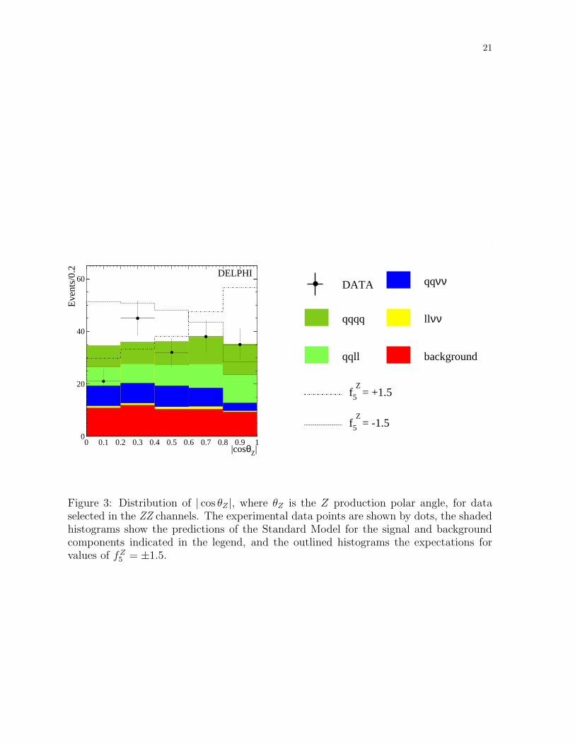
Figure 3 shows the distribution of | cos θZ | for a high purity sample of ZZ data, com-posed of the qql+l− and l+l−νν samples defined above and, for illustrative purposes,samples of qqqq and qqνν events defined by stringent cuts on the probabilistic variablesused in these channels (qqqq probability > 0.55, and qqνν IDA variable > 3), so as tosuppress the background levels present. (As described below, no cuts were imposed onthese variables in the determination of coupling parameters). The figure also shows the

10

Standard Model expectations and the distributions predicted for values of fZ5 = ±1.5.

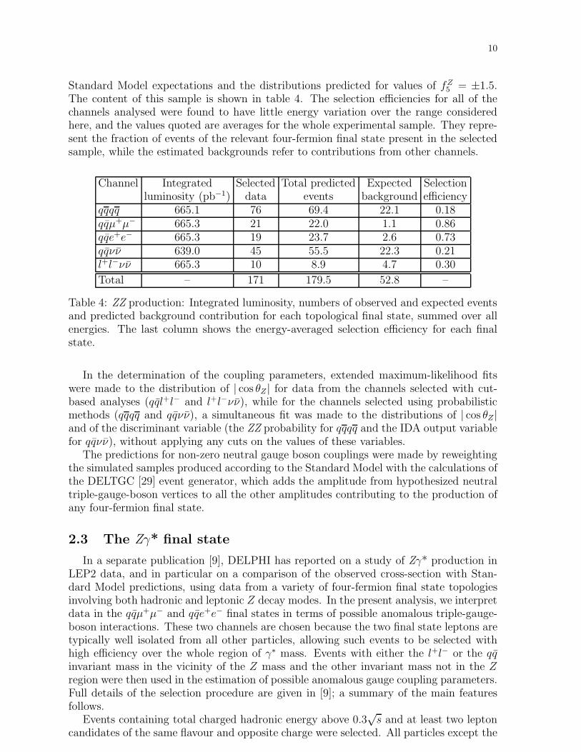
The content of this sample is shown in table 4. The selection efficiencies for all of thechannels analysed were found to have little energy variation over the range consideredhere, and the values quoted are averages for the whole experimental sample. They repre-sent the fraction of events of the relevant four-fermion final state present in the selectedsample, while the estimated backgrounds refer to contributions from other channels.

Channel Integrated Selected Total predicted Expected Selectionluminosity (pb−1) data events background efficiency

qqqq 665.1 76 69.4 22.1 0.18qqµ+µ− 665.3 21 22.0 1.1 0.86qqe+e− 665.3 19 23.7 2.6 0.73qqνν 639.0 45 55.5 22.3 0.21l+l−νν 665.3 10 8.9 4.7 0.30

Total – 171 179.5 52.8 –

Table 4: ZZ production: Integrated luminosity, numbers of observed and expected eventsand predicted background contribution for each topological final state, summed over allenergies. The last column shows the energy-averaged selection efficiency for each finalstate.

In the determination of the coupling parameters, extended maximum-likelihood fitswere made to the distribution of | cos θZ | for data from the channels selected with cut-based analyses (qql+l− and l+l−νν), while for the channels selected using probabilisticmethods (qqqq and qqνν), a simultaneous fit was made to the distributions of | cos θZ |and of the discriminant variable (the ZZ probability for qqqq and the IDA output variablefor qqνν), without applying any cuts on the values of these variables.

The predictions for non-zero neutral gauge boson couplings were made by reweightingthe simulated samples produced according to the Standard Model with the calculations ofthe DELTGC [29] event generator, which adds the amplitude from hypothesized neutraltriple-gauge-boson vertices to all the other amplitudes contributing to the production ofany four-fermion final state.

2.3 The Zγ* final state

In a separate publication [9], DELPHI has reported on a study of Zγ* production inLEP2 data, and in particular on a comparison of the observed cross-section with Stan-dard Model predictions, using data from a variety of four-fermion final state topologiesinvolving both hadronic and leptonic Z decay modes. In the present analysis, we interpretdata in the qqµ+µ− and qqe+e− final states in terms of possible anomalous triple-gauge-boson interactions. These two channels are chosen because the two final state leptons aretypically well isolated from all other particles, allowing such events to be selected withhigh efficiency over the whole region of γ∗ mass. Events with either the l+l− or the qqinvariant mass in the vicinity of the Z mass and the other invariant mass not in the Zregion were then used in the estimation of possible anomalous gauge coupling parameters.Full details of the selection procedure are given in [9]; a summary of the main featuresfollows.

Events containing total charged hadronic energy above 0.3√s and at least two lepton

candidates of the same flavour and opposite charge were selected. All particles except the

11

lepton candidates were clustered into jets and a kinematic fit requiring four-momentumconservation was applied. At least one of the two lepton candidates was required tosatisfy strong lepton identification criteria, while softer requirements were specified forthe second. In order to increase the purity of the selection, further cuts were made intwo discriminating variables: Pmin

t , the lesser of the transverse momenta of the leptoncandidates with respect to their nearest jet, and the χ2 per degree of freedom of thekinematic fit. This procedure selected a total of 170 events in the combined qqµ+µ− andqqe+e− channels. The Zγ∗ sample was then defined within the selected qql+l− data byrequiring the mass of one and only one f f pair to be in the Z region. This was effected byimposing mass cuts in the (Mhadrons,Mµ+µ−) and (Mhadrons,Me+e−) planes, whereMhadrons

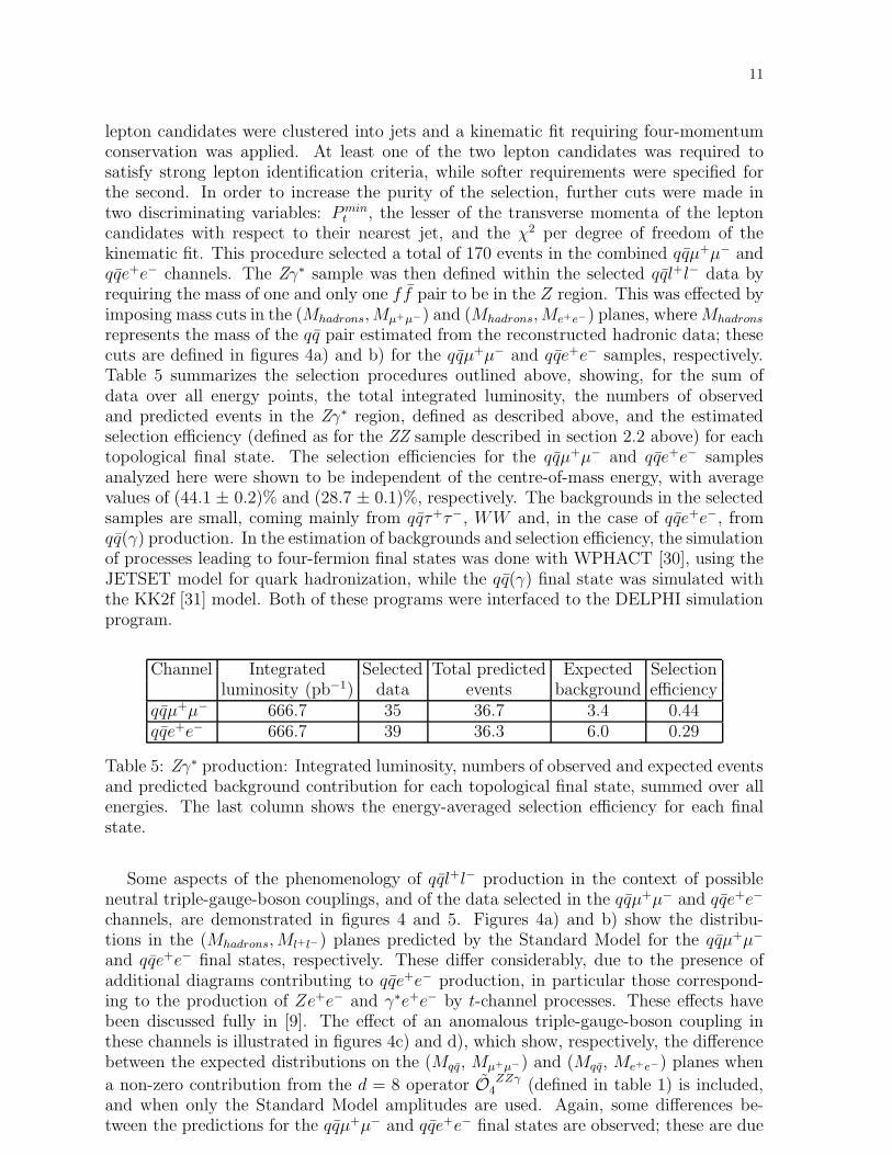
represents the mass of the qq pair estimated from the reconstructed hadronic data; thesecuts are defined in figures 4a) and b) for the qqµ+µ− and qqe+e− samples, respectively.Table 5 summarizes the selection procedures outlined above, showing, for the sum ofdata over all energy points, the total integrated luminosity, the numbers of observedand predicted events in the Zγ∗ region, defined as described above, and the estimatedselection efficiency (defined as for the ZZ sample described in section 2.2 above) for eachtopological final state. The selection efficiencies for the qqµ+µ− and qqe+e− samplesanalyzed here were shown to be independent of the centre-of-mass energy, with averagevalues of (44.1 ± 0.2)% and (28.7 ± 0.1)%, respectively. The backgrounds in the selectedsamples are small, coming mainly from qqτ+τ−, WW and, in the case of qqe+e−, fromqq(γ) production. In the estimation of backgrounds and selection efficiency, the simulationof processes leading to four-fermion final states was done with WPHACT [30], using theJETSET model for quark hadronization, while the qq(γ) final state was simulated withthe KK2f [31] model. Both of these programs were interfaced to the DELPHI simulationprogram.

Channel Integrated Selected Total predicted Expected Selectionluminosity (pb−1) data events background efficiency

qqµ+µ− 666.7 35 36.7 3.4 0.44qqe+e− 666.7 39 36.3 6.0 0.29

Table 5: Zγ∗ production: Integrated luminosity, numbers of observed and expected eventsand predicted background contribution for each topological final state, summed over allenergies. The last column shows the energy-averaged selection efficiency for each finalstate.

Some aspects of the phenomenology of qql+l− production in the context of possibleneutral triple-gauge-boson couplings, and of the data selected in the qqµ+µ− and qqe+e−

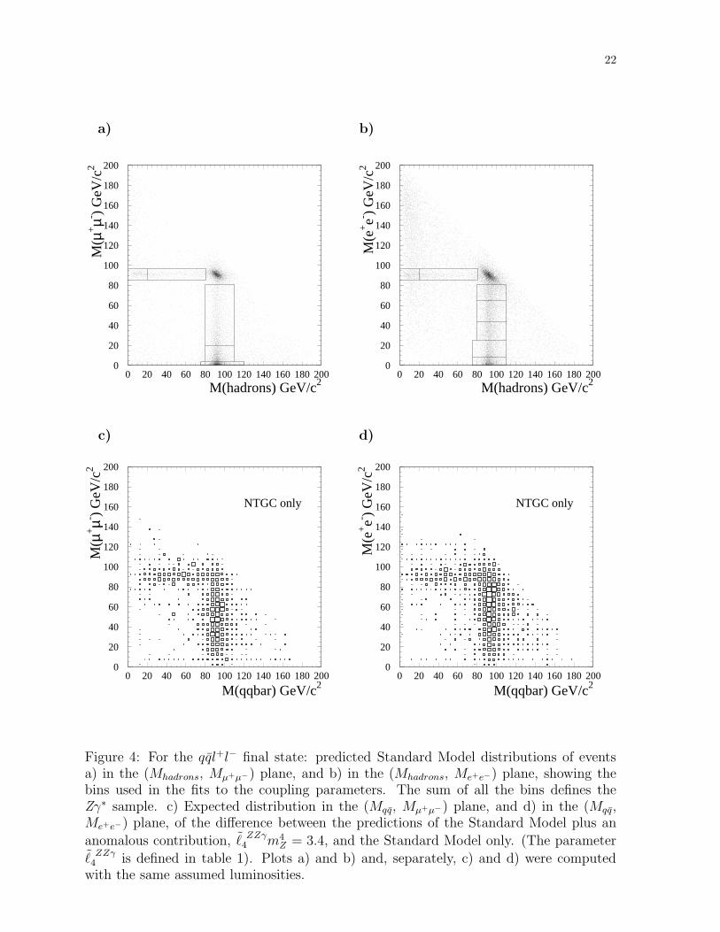
channels, are demonstrated in figures 4 and 5. Figures 4a) and b) show the distribu-tions in the (Mhadrons,Ml+l−) planes predicted by the Standard Model for the qqµ+µ−

and qqe+e− final states, respectively. These differ considerably, due to the presence ofadditional diagrams contributing to qqe+e− production, in particular those correspond-ing to the production of Ze+e− and γ∗e+e− by t-channel processes. These effects havebeen discussed fully in [9]. The effect of an anomalous triple-gauge-boson coupling inthese channels is illustrated in figures 4c) and d), which show, respectively, the differencebetween the expected distributions on the (Mqq, Mµ+µ−) and (Mqq, Me+e−) planes when

a non-zero contribution from the d = 8 operator O ZZγ4 (defined in table 1) is included,

and when only the Standard Model amplitudes are used. Again, some differences be-tween the predictions for the qqµ+µ− and qqe+e− final states are observed; these are due

12

to the presence of additional diagrams in the qqe+e− amplitude, in this case the V 0V 0

fusion diagram leading to Ze+e− production, shown in figure 1d). The overall effect is anegative interference between s- and t-channel amplitudes: for the example shown, thepredicted content of figure 4d) (qqe+e−) is ∼ 40% of that of the qqµ+µ− prediction.

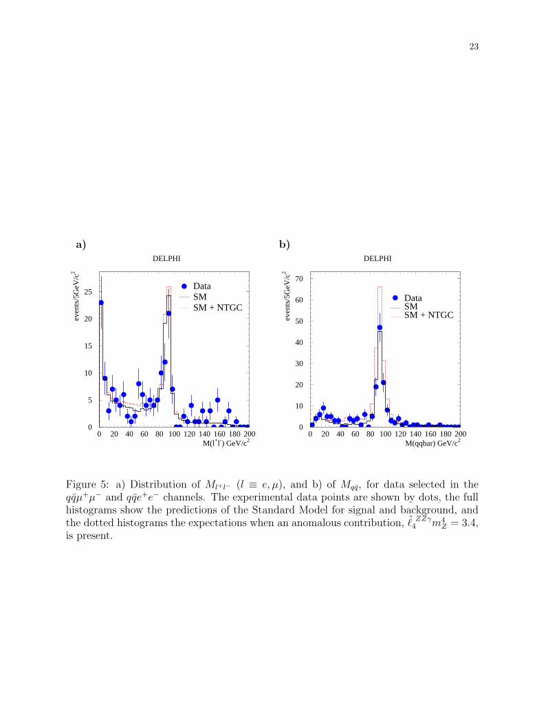
Data selected over the whole region of the qql+l− phase space are presented in fig-ures 5a) and b) in the form of the distributions of Ml+l− (l ≡ µ, e) and Mqq. These plotsalso show the expectations of the Standard Model and of a model in which an anomalouscontribution ℓ ZZγ

4 m4Z = 3.4 from the operator O ZZγ

4 is present.In the determination of the coupling parameters, the regions in the plane of the masses

of the two fermion-antifermion pairs defining the Zγ∗ samples in the qqµ+µ− and qqe+e−

final states, shown in figures 4a) and b), respectively, were divided into a small numberof bins of unequal size, but containing roughly equal numbers of events predicted by theStandard Model. Different bin definitions were made for the two channels; the bins arealso defined in the figures, and they correspond to those used by DELPHI in [9] in thedetermination of the Zγ∗ cross-section. In [9], each of the mass bins defined for the qqe+e−

event sample was further divided into two angular regions, (40◦ < θl+l− < 140◦) and(θl+l− < 40◦ or θl+l− > 140◦), where θl+l− is the polar angle of the final state e+e− systemwith respect to the beam direction. These angular regions correspond to DELPHI’s barreland endcap regions, respectively. In the present analysis, we have extended this divisionto apply to muon as well as electron pairs in the qql+l− final states. Binned likelihood fitsto the couplings were then made with the bins in (Mqq,Ml+l−) and θl+l− thus defined. Asin the case of the ZZ final state previously described, the predictions for non-zero neutralgauge boson couplings in the Zγ∗ data were made by reweighting the simulated samplesproduced according to the Standard Model with the calculations of DELTGC.

3 Results

In this section the results of our study are presented, expressed in terms of the param-eters listed in table 1 describing the neutral triple-gauge-boson effective Lagrangian. Insummary, these parameters represent:

a) the coefficients of the lowest dimension operators contributing to production eitherof the ZZ and Zγ∗ final states, or to production of the Zγ, Zγ∗ and ZZ final states;in the on-shell ZZ or Zγ limit each of these parameters becomes equal to one of theon-shell coefficients fV

i or hVi ;

b) the coefficients of the lowest dimension operators affecting only the V 0Zγ∗ vertex;c) the coefficients of the SU(2) × U(1)-conserving operators describing the V 0

1 V02 V

03

vertex in i) the Gounaris-Layssac-Renard and ii) the Alcaraz formulations.

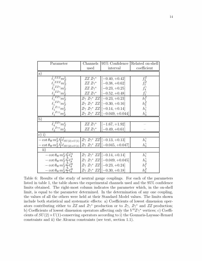
The labels a), b), c) above refer to table 1.Limits on the parameters at the 95% confidence level are given in table 6 and the

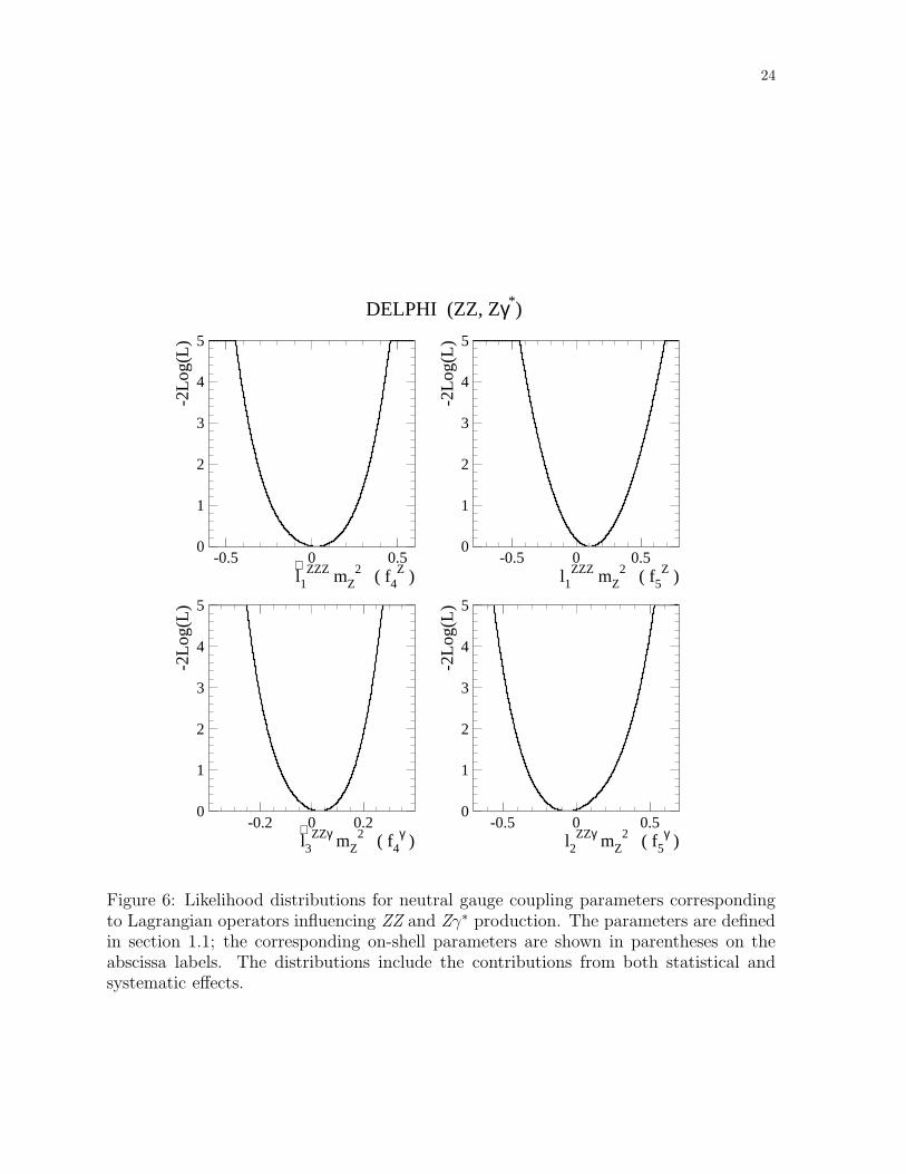
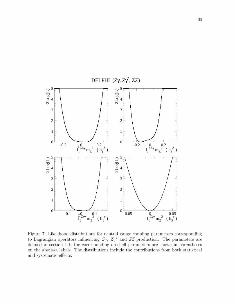
corresponding likelihood curves are shown in figures 6-10. In all cases, the values quotedare derived from one-parameter fits to the data in the Zγ, ZZ and Zγ∗ channels describedin sections 2.1, 2.2 and 2.3 above, summing the distributions from different channelswhere appropriate. In each fit, the values of the other parameters were set to zero, theirStandard Model value. The results shown include contributions from both statistical andsystematic effects.

For reference, we summarize here the composition of the likelihood function from eachof the final states used in the analysis, described in more detail in the sections above:In the Zγ → ννγ channel, the number of events with a high energy photon emitted at

13

large polar angle was used in the fit, while in the Zγ→ qqγ channel the fit was performedto the distribution of the decay angle of the Z in its rest frame. In the channels ZZ →qql+l− and ZZ → l+l−νν the distribution of the Z production angle was fitted; in ZZ→ qqqq and ZZ → qqνν simultaneous fits were made to the Z production angle and,respectively, to the event probability or discriminant variable distributions. In the Zγ∗

channels studied (Zγ∗ → qqµ+µ− and Zγ∗ → qqe+e−) the likelihood was evaluated inbins of qq or l+l− mass and of the polar angle of the detected l+l− system.

It may be noted that, in the models conventionally used to describe anomalous gauge-boson couplings, including the one used in this paper, all observables have a quadraticdependence on the fitted parameters. This effect, which has been previously noted (see,for example, [10]), leads to log-likelihood distributions which can have double mimima,asymmetries, and a broadening compared with that expected in the Gaussian case. Suchfeatures are indeed seen in several of the plots in figures 6-10. The confidence limitsreported in table 6 must therefore be interpreted with this effect in mind.

3.1 Systematic errors

In the determination of the confidence limits shown in table 6 and the likelihood curvesof figures 6-10, several sources of systematic error were considered for each of the finalstates included in the study. These are described below.

In the ννγ and qqγ channels contributing to Zγ production, uncertainties of ±1% wereassumed in the values assumed for the Standard Model production cross-sections [17,18],and an experimental uncertainty of ±1% was assumed for the energy calibration of theelectromagnetic calorimeter. The effect of an uncertainty of ±1% in the luminosity mea-surement was also computed, while the uncertainties in the calculations arising from thefinite simulated statistics in signal and background channels and from the uncertaintyin the knowledge of the background cross-section were found to be negligible in bothchannels. In the ννγ channel, the error due to the uncertainty of ±3% in the triggerefficiency was included. In the qqγ channel, the uncertainty in the use of PYTHIA asthe hadronization model was taken into account by comparing events simulated withPYTHIA and HERWIG [32]; this gave rise to an estimated systematic error on the selec-tion efficiency of ±1.7% from this source. In the combination of data at different energies,all the above effects were considered as correlated. The resulting overall systematic errorin the coupling parameters was found to be of the order of 30% of the statistical errors inthe case of hZ

1 and hZ3 , about 50% of the statistical error for hγ

1 , and of the same order asthe statistical error for hγ

3 . In combination with Zγ∗ and ZZ data to produce the limitson the parameters ℓ ZZγ

1 m2Z , ℓ

ZZγ1 m2

Z , ℓZγγ1 m2

Z and ℓ Zγγ1 m2

Z shown in table 6a) the Zγdata dominate (see sections 1.1 and 3.2 for further discussion of this point), so that theratios of systematic to statistical errors quoted above are also applicable to the respective

ℓV 01V 02V 03

i m2Z results reported in the table.

A full description of the treatment of systematic effects in the channels contributingto ZZ production has been given in [8]. In the qqqq channel, the dominant effect arisesfrom uncertainties in the modelling of the main source of background, namely productionof the qq(γ) final state, when the subsequent hadronization of the quarks gives rise toseveral jets. In the present study, the effect of this background was estimated by assumingan uncertainty of ±5% in the qq(γ) production cross-section. In the qql+l− channel, thedominant systematic effect relevant to the present study comes from the uncertainty inthe efficiency for selecting qqe+e− and qqµ+µ− events, taken to be ±3%. In addition,in the qqe+e− channel a relative uncertainty of ±15% was estimated in the calculation

14

Parameter Channels 95% Confidence Related on-shellused interval coefficient

a)

ℓ ZZZ1 m2

Z ZZ Zγ∗ [−0.40,+0.42] fZ4

ℓ ZZZ1 m2

Z ZZ Zγ∗ [−0.38,+0.62] fZ5

ℓ ZZγ3 m2

Z ZZ Zγ∗ [−0.23,+0.25] f γ4

ℓ ZZγ2 m2

Z ZZ Zγ∗ [−0.52,+0.48] f γ5

ℓ ZZγ1 m2

Z Zγ Zγ∗ ZZ [−0.23,+0.23] hZ1

ℓ ZZγ1 m2

Z Zγ Zγ∗ ZZ [−0.30,+0.16] hZ3

ℓ Zγγ1 m2

Z Zγ Zγ∗ ZZ [−0.14,+0.14] hγ1

ℓ Zγγ1 m2

Z Zγ Zγ∗ ZZ [−0.049,+0.044] hγ3

b)

ℓ ZZγ4 m4

Z ZZ Zγ∗ [−1.67,+1.92] –

ℓ Zγγ2 m4

Z ZZ Zγ∗ [−0.49,+0.61] –

c) i)

− cot θWm2Z

v2

4ℓSU(2)×U(1) Zγ Zγ∗ ZZ [−0.13,+0.13] hγ

1

− cot θWm2Z

v2

4ℓSU(2)×U(1) Zγ Zγ∗ ZZ [−0.045,+0.047] hγ

3

ii)

− cot θWm2Z

v2

4ℓA8 Zγ Zγ∗ ZZ [−0.14,+0.14] hγ

1

− cot θWm2Z

v2

4ℓA8 Zγ Zγ∗ ZZ [−0.049,+0.045] hγ

3

− cot θWm2Z

v2

4ℓB8 Zγ Zγ∗ ZZ [−0.23,+0.24] hZ

1

− cot θWm2Z

v2

4ℓB8 Zγ Zγ∗ ZZ [−0.30,+0.18] hZ

3

Table 6: Results of the study of neutral gauge couplings. For each of the parameterslisted in table 1, the table shows the experimental channels used and the 95% confidencelimits obtained. The right-most column indicates the parameter which, in the on-shelllimit, is equal to the parameter determined. In the determination of any one coupling,the values of all the others were held at their Standard Model values. The limits showninclude both statistical and systematic effects: a) Coefficients of lowest dimension oper-ators contributing either to ZZ and Zγ∗ production or to Zγ, Zγ∗ and ZZ production;b) Coefficients of lowest dimension operators affecting only the V 0Zγ∗ vertices; c) Coeffi-cients of SU(2)×U(1)-conserving operators according to i) the Gounaris-Layssac-Renardconstraints and ii) the Alcaraz constraints (see text, section 1.1).

15

of the background level. In the qqνν channel, as in qqqq, the main source of systematicerror arises from modelling of the qq(γ) background, in this case corresponding to thekinematic region with large missing energy, and hence low visible qq energy. A study ofthe energy flow in this region using events at the Z peak allowed a determination of theeffect of this uncertainty in the present analysis; it gives rise to systematic errors in thecoupling parameters of order 5% - 10% of the values of the statistical errors. Another,comparable source of systematic error in this channel comes from the uncertainties inthe cross-sections for the dominant background channels, particularly Weν production.Systematic effects in the l+l−νν channels were found to be negligible. In addition, theeffects of uncertainties of±2% in the overall ZZ cross-section and of±1% in the luminositymeasurement were considered. The combined effect of all the systematic uncertainties inthe channels contributing to ZZ production is small, typically ∼ 15% of the statisticalerrors, and, as in the case of the hV

i -related parameters discussed above, this ratio of

systematic to statistical effects is also applicable to the results for the ℓV 01V 02V 03

i m2Z related

to on-shell fVi parameters shown in table 6a).

The systematic uncertainties in the study of the qqe+e− and qqµ+µ− channels con-tributing to Zγ∗ production have been described in [9]. Several effects, including uncer-tainties in lepton identification, the effect of limited simulated data and, in the qqe+e−

channel, identification of fake electrons coming from background channels, combine togive a systematic error on the efficiency to select qqe+e− and qqµ+µ− events of ±5% anda relative uncertainty in the background level of ±15%. In addition, a systematic error of±1% in the luminosity measurement was assumed. The overall effect of these systematicuncertainties in the determination of the coupling parameters is small in comparison withthe statistical errors. In combination with ZZ data to produce the results for parametersℓ Zγγ2 and ℓ ZZγ

4 listed in table 6b), they amount to ∼15% and ∼5% of the statisticalerrors, respectively.

In the combination of data from the different final states, Zγ, ZZ and Zγ∗, all thesystematic effects listed above were treated as uncorrelated except those arising from theuncertainty in the luminosity measurement.

3.2 Discussion

A few comments may be made on the results shown in table 6 and figures 6-10.All the results are compatible with the Standard Model expectation of the absence of

neutral triple-gauge-boson couplings. The results shown in table 6a) and figures 6 and 7demonstrate this conclusion in the effective Lagrangian model of reference [2] for thed = 6 operators which, in the on-shell limit, contribute either to ZZ or to Zγ production.As mentioned in sections 1.1 and 3.1 (and predicted from studies of simulated events [6]),the contribution to these results of the off-shell data included in their determination issmall: using only the off-shell data leads to precisions poorer by factors of ∼ 3− 7 thanusing the on-shell Zγ or ZZ data. (This effect is observed most strongly in the case of thedetermination of hγ

3 , where the interference in the squared matrix element between theanomalous and Standard Model amplitudes leads to a relatively precise determinationof this parameter). Thus these results, with negligible changes, may also be interpretedin terms of the parameters hV

i and fVi of on-shell Zγ and ZZ production, listed in the

right-hand column of the table, and they may be compared directly with other publishedresults for these on-shell parameters.

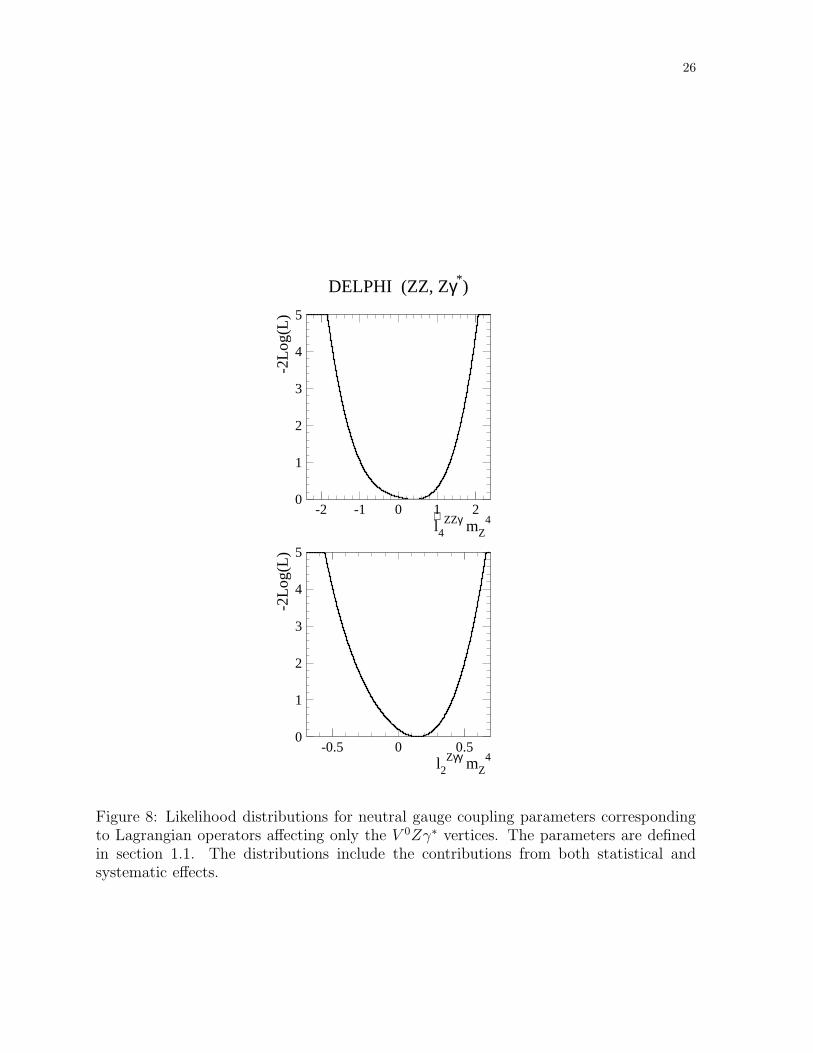
The results shown in table 6b) and figure 8 examine the possibility of four-fermionproduction via an anomalous V 0Zγ∗ vertex by determining the coefficients of the lowest

16

dimension (d = 8) operators in the model of reference [2] which would contribute to sucha process. As noted in section 1.1, contributions from these operators affect both theZγ∗ and ZZ final states; in the determination of ℓ Zγγ

2 , the experimental samples fromthe two final states contribute roughly equally to the log likelihood distribution in thecombination of data, while in the determination of ℓ ZZγ

4 the Zγ∗ contribution dominates.The results of the fits show that there is no evidence in the data for a CP -conservinganomalous coupling at the γZγ∗ vertex or for a CP -violating coupling at the ZZγ∗

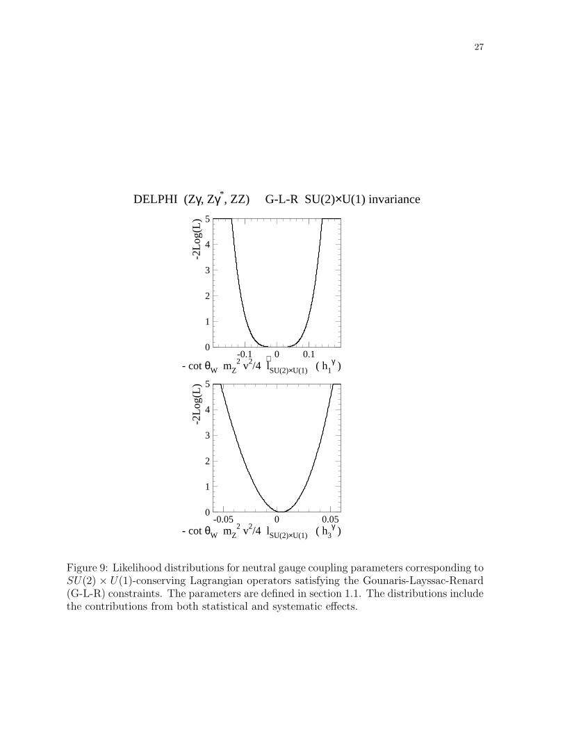
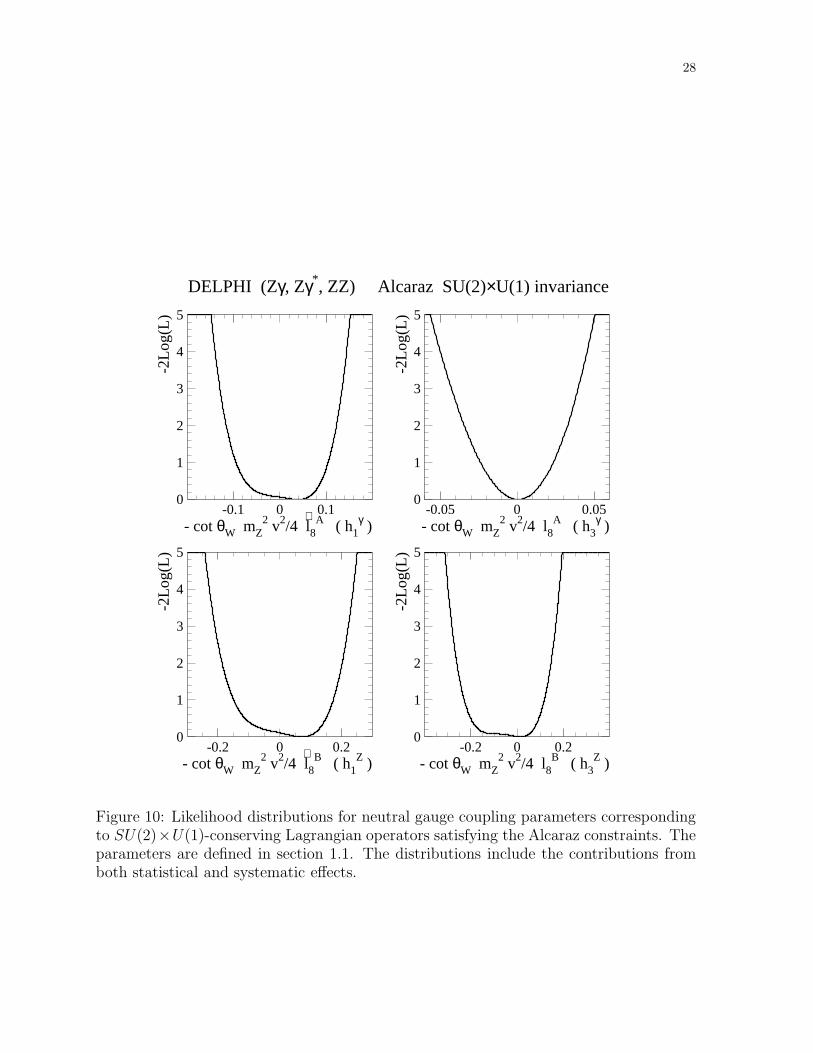
vertex.The results shown in table 6c) and figures 9 and 10 indicate that there is no evidence in

the data for SU(2)×U(1)-conserving anomalous couplings in the models of references [2]and [6]. Here again, in the combinations of data from different final states, the contri-butions from Zγ production dominate, as can be seen by comparison of the likelihoodcurves of figure 7 and either figure 9 or figure 10, and from the confidence limits shownin the table. This arises both because of the sensitivity to hγ

3 noted above and becauseof the greater statistical contribution from Zγ compared to that from ZZ production atLEP2 energies.

4 Conclusions

A study has been performed of the neutral triple-gauge-boson vertex using DELPHIdata from the final states Zγ, ZZ and Zγ∗ produced at LEP2. The results have beeninterpreted in terms of various models of the interaction Lagrangian proposed in theliterature. We find no evidence for the production of these states by processes involvingneutral triple-gauge-boson vertices with either one or two off-shell bosons, nor when thedata are analyzed in terms of models in which the neutral triple-gauge-boson vertex isconstrained to be SU(2)×U(1)-conserving. These conclusions are in agreement with thepredictions of the Standard Model.

Acknowledgements

We are greatly indebted to our technical collaborators, to the members of the CERN-SL Division for the excellent performance of the LEP collider, and to the funding agenciesfor their support in building and operating the DELPHI detector.We acknowledge in particular the support ofAustrian Federal Ministry of Education, Science and Culture, GZ 616.364/2-III/2a/98,FNRS–FWO, Flanders Institute to encourage scientific and technological research in theindustry (IWT) and Belgian Federal Office for Scientific, Technical and Cultural affairs(OSTC), Belgium,FINEP, CNPq, CAPES, FUJB and FAPERJ, Brazil,Ministry of Education of the Czech Republic, project LC527,Academy of Sciences of the Czech Republic, project AV0Z10100502,Commission of the European Communities (DG XII),Direction des Sciences de la Matiere, CEA, France,Bundesministerium fur Bildung, Wissenschaft, Forschung und Technologie, Germany,General Secretariat for Research and Technology, Greece,National Science Foundation (NWO) and Foundation for Research on Matter (FOM),The Netherlands,Norwegian Research Council,

17

State Committee for Scientific Research, Poland, SPUB-M/CERN/PO3/DZ296/2000,SPUB-M/CERN/PO3/DZ297/2000, 2P03B 104 19 and 2P03B 69 23(2002-2004)FCT - Fundacao para a Ciencia e Tecnologia, Portugal,Vedecka grantova agentura MS SR, Slovakia, Nr. 95/5195/134,Ministry of Science and Technology of the Republic of Slovenia,CICYT, Spain, AEN99-0950 and AEN99-0761,The Swedish Research Council,Particle Physics and Astronomy Research Council, UK,Department of Energy, USA, DE-FG02-01ER41155,EEC RTN contract HPRN-CT-00292-2002.

18

References

[1] K. Hagiwara et al., Nucl. Phys. B282 (1987) 253.[2] G.J. Gounaris, J. Layssac and F.M. Renard, Phys. Rev. D62 (2000) 073012.[3] M.S. Bilenky et al., Nucl. Phys. B409 (1993) 22.[4] G. Gounaris et al., in Physics at LEP2, eds. G. Altarelli, T. Sjostrand and F. Zwirner,

CERN 96-01 (1996) Vol.1, 525.[5] G.J. Gounaris, J. Layssac and F.M. Renard, addendum to [2] above, in hep-

ph/0005269 (2000).[6] J. Alcaraz, Phys. Rev. D65 (2002) 075020.[7] DELPHI Collaboration, W. Adam et al., Phys. Lett. B380 (1996) 471;

DELPHI Collaboration, P. Abreu et al., Phys. Lett. B423 (1998) 194.[8] DELPHI Collaboration, J. Abdallah et al., Eur. Phys. J. C30 (2003) 447.[9] DELPHI Collaboration, J. Abdallah et al., Zγ∗ production in e+e− interactions at√

s = 183 - 209 GeV, Accepted by Eur. Phys. J. C, arXiv:0706.2565[10] OPAL Collaboration G. Abbiendi et al., Eur. Phys. J. C17 (2000) 553.[11] ALEPH Collaboration, ALEPH 2001-061 CONF 2001-041 (2001);

L3 Collaboration, P. Achard et al., Phys. Lett. B572 (2003) 133;L3 Collaboration, P. Achard et al., Phys. Lett. B597 (2004) 119;OPAL Collaboration, G. Abbiendi et al., Eur. Phys. J. C32 (2004) 303.

[12] DELPHI Collaboration, P. Aarnio et al., Nucl. Instr. and Meth. A303 (1991) 233.[13] DELPHI Collaboration, P. Abreu et al., Nucl. Instr. and Meth. A378 (1996) 57.[14] DELPHI Trigger Group, A. Augustinus et al., Nucl. Instr. and Meth. A515 (2003)

782.[15] DELPHI Silicon Tracker Group, P. Chochula et al., Nucl. Instr. and Meth. A412

(1998) 304.[16] DELPHI Collaboration, J. Abdallah et al., Eur. Phys. J. C38 (2005) 395.[17] G. Montagna et al., Nucl. Phys. B452 (1995) 161.[18] S. Jadach, B.F.L. Ward and Z. Was, Comp. Phys. Comm. 79 (1994) 503.[19] P. Abreu et al., Nucl. Instr. and Meth. A427 (1999) 487.[20] T.Sjostrand, PYTHIA 5.7 / JETSET 7.4, CERN-TH 7112/93 (1993).[21] U. Baur and E.L. Berger, Phys. Rev. D47 (1993) 4889.[22] G.J. Gounaris, J. Layssac and F.M. Renard, Phys. Rev. D61 (2000) 073013.[23] T.G.M. Malmgren, Comp. Phys. Comm. 106 (1997) 230;

T.G.M. Malmgren and K.E. Johansson, Nucl. Instr. and Meth. 403 (1998) 481.[24] F.A. Berends, R. Pittau and R. Kleiss, Comp. Phys. Comm. 85 (1995) 437.[25] J. Fujimoto et al., Comp. Phys. Comm. 100 (1997) 128.[26] S. Jadach, W. Placzek and B.F.L. Ward, Phys. Lett. B390 (1997) 298.[27] T. Alderweireld et al., in Reports of the Working Groups on Precision Calculations

for LEP2 Physics, eds. S. Jadach, G. Passarino and R. Pittau, CERN 2000-009(2000) 219.

[28] F.A. Berends, P.H. Daverveldt and R. Kleiss, Comp. Phys. Comm. 40 (1986) 271,285 and 309.

[29] O.P. Yushchenko and V.V. Kostyukhin, DELTGC - A program for four-fermioncalculations, DELPHI 99-4 PHYS 816 (1999).

[30] E. Accomando and A. Ballestrero, Comp. Phys. Comm. 99 (1997) 270;E. Accomando, A. Ballestrero and E. Maina, Comp. Phys. Comm. 150 (2003) 166;A. Ballestrero, R. Chierici, F. Cossutti and E. Migliore, Comp. Phys. Comm. 152(2003) 175.

19

[31] S. Jadach, B.F.L. Ward and Z. Was, Comp. Phys. Comm. 130 (2000) 260.[32] G. Marchesini et al., Comp. Phys. Comm. 67 (1992) 465.

20

0

10

20

30

40

50

60

70

80

0 0.2 0.4 0.6 0.8 1 1.2xγ

even

ts/.0

5

γνν

DATA

a)DELPHI

0

25

50

75

100

125

150

175

200

225

250

0 0.1 0.2 0.3 0.4 0.5 0.6 0.7 0.8 0.9 1|cosα*|

Eve

nts/

0.1

DELPHI

h3 γ = -0.2

h3 γ = +0.2

background

qqγ

● DATA

h3 γ = -0.2

h3 γ = +0.2

h3 γ = -0.2

h3 γ = +0.2

background

qqγ

● DATA

h3 γ = -0.2

h3 γ = +0.2

h3 γ = -0.2

h3 γ = +0.2

background

qqγ

● DATA

h3 γ = -0.2

h3 γ = +0.2

••

b)

Figure 2: a) Distribution of xγ = Eγ/Ebeam, the energy of identified photons normal-ized to the beam energy in the data in the ννγ channel, summed over all energy points.The distribution is shown before imposing the experimental cut at Eγ = 50 GeV. Theexperimental data points are shown by dots and the shaded histogram shows the predic-tions of the Standard Model for signal plus background. (The background contributionis very small, and is not shown separately). b) Distribution of | cosα⋆|, where α⋆ is thedecay angle of the quark (or antiquark) in the Z centre-of-mass frame with respect tothe direction of the Z in the overall centre of mass, for data selected in the qqγ channel.The experimental data points are shown by dots, the shaded histogram shows the pre-dictions of the Standard Model for signal and background, and the outlined histogramsthe expectations for values of hγ

3 = ±0.2.

21

0

20

40

60

0 0.1 0.2 0.3 0.4 0.5 0.6 0.7 0.8 0.9 1|cosθZ|

Eve

nts/

0.2

DELPHI

background

llνν

qqνν

qqll

qqqq

● DATA

f5 Z = -1.5

f5 Z = +1.5

Figure 3: Distribution of | cos θZ |, where θZ is the Z production polar angle, for dataselected in the ZZ channels. The experimental data points are shown by dots, the shadedhistograms show the predictions of the Standard Model for the signal and backgroundcomponents indicated in the legend, and the outlined histograms the expectations forvalues of fZ

5 = ±1.5.

22

0

20

40

60

80

100

120

140

160

180

200

0 20 40 60 80 100 120 140 160 180 200

M(hadrons) GeV/c2

M(µ

+µ- )

GeV

/c2

0

20

40

60

80

100

120

140

160

180

200

0 20 40 60 80 100 120 140 160 180 200

M(hadrons) GeV/c2M

(e+e- )

GeV

/c2

0

20

40

60

80

100

120

140

160

180

200

0 20 40 60 80 100 120 140 160 180 200

NTGC only

M(qqbar) GeV/c2

M(µ

+µ- )

GeV

/c2

0

20

40

60

80

100

120

140

160

180

200

0 20 40 60 80 100 120 140 160 180 200

NTGC only

M(qqbar) GeV/c2

M(e

+e- )

GeV

/c2

a) b)

c) d)

Figure 4: For the qql+l− final state: predicted Standard Model distributions of eventsa) in the (Mhadrons, Mµ+µ−) plane, and b) in the (Mhadrons, Me+e−) plane, showing thebins used in the fits to the coupling parameters. The sum of all the bins defines theZγ∗ sample. c) Expected distribution in the (Mqq, Mµ+µ−) plane, and d) in the (Mqq,Me+e−) plane, of the difference between the predictions of the Standard Model plus an

anomalous contribution, ℓ ZZγ4 m4

Z = 3.4, and the Standard Model only. (The parameter

ℓ ZZγ4 is defined in table 1). Plots a) and b) and, separately, c) and d) were computedwith the same assumed luminosities.

23

DELPHI

0

5

10

15

20

25

0 20 40 60 80 100 120 140 160 180 200M(l+l-) GeV/c2

even

ts/5

GeV

/c2

DataSMSM + NTGC

DELPHI

0

10

20

30

40

50

60

70

0 20 40 60 80 100 120 140 160 180 200M(qqbar) GeV/c2

even

ts/5

GeV

/c2

DataSMSM + NTGC

a) b)

Figure 5: a) Distribution of Ml+l− (l ≡ e, µ), and b) of Mqq, for data selected in theqqµ+µ− and qqe+e− channels. The experimental data points are shown by dots, the fullhistograms show the predictions of the Standard Model for signal and background, andthe dotted histograms the expectations when an anomalous contribution, ℓ ZZγ

4 m4Z = 3.4,

is present.

24

DELPHI (ZZ, Zγ*)

0

1

2

3

4

5

-0.5 0 0.5l∼1 ZZZ mZ

2 ( f4 Z )

-2L

og(L

)

0

1

2

3

4

5

-0.5 0 0.5l1

ZZZ mZ 2 ( f5

Z )

-2L

og(L

)

0

1

2

3

4

5

-0.2 0 0.2l∼3 ZZγ mZ

2 ( f4 γ )

-2L

og(L

)

0

1

2

3

4

5

-0.5 0 0.5l2

ZZγ mZ 2 ( f5

γ )

-2L

og(L

)

Figure 6: Likelihood distributions for neutral gauge coupling parameters correspondingto Lagrangian operators influencing ZZ and Zγ∗ production. The parameters are definedin section 1.1; the corresponding on-shell parameters are shown in parentheses on theabscissa labels. The distributions include the contributions from both statistical andsystematic effects.

25

DELPHI (Zγ, Zγ*, ZZ)

0

1

2

3

4

5

-0.2 0 0.2l∼1 ZZγ mZ

2 ( h1 Z )

-2L

og(L

)

0

1

2

3

4

5

-0.2 0 0.2l1

ZZγ mZ 2 ( h3

Z )

-2L

og(L

)

0

1

2

3

4

5

-0.1 0 0.1l∼1 Zγγ mZ

2 ( h1 γ )

-2L

og(L

)

0

1

2

3

4

5

-0.05 0 0.05l1

Zγγ mZ 2 ( h3

γ )

-2L

og(L

)

Figure 7: Likelihood distributions for neutral gauge coupling parameters correspondingto Lagrangian operators influencing Zγ, Zγ∗ and ZZ production. The parameters aredefined in section 1.1; the corresponding on-shell parameters are shown in parentheseson the abscissa labels. The distributions include the contributions from both statisticaland systematic effects.

26

DELPHI (ZZ, Zγ*)

0

1

2

3

4

5

-2 -1 0 1 2l∼4 ZZγ mZ

4

-2L

og(L

)

0

1

2

3

4

5

-0.5 0 0.5l2

Zγγ mZ 4

-2L

og(L

)

Figure 8: Likelihood distributions for neutral gauge coupling parameters correspondingto Lagrangian operators affecting only the V 0Zγ∗ vertices. The parameters are definedin section 1.1. The distributions include the contributions from both statistical andsystematic effects.

27

DELPHI (Zγ, Zγ*, ZZ) G-L-R SU(2)×U(1) invariance

0

1

2

3

4

5

-0.1 0 0.1- cot θW mZ

2 v 2/4 l∼SU(2)×U(1) ( h1

γ )

-2L

og(L

)

0

1

2

3

4

5

-0.05 0 0.05- cot θW mZ

2 v 2/4 lSU(2)×U(1) ( h3 γ )

-2L

og(L

)

Figure 9: Likelihood distributions for neutral gauge coupling parameters corresponding toSU(2) × U(1)-conserving Lagrangian operators satisfying the Gounaris-Layssac-Renard(G-L-R) constraints. The parameters are defined in section 1.1. The distributions includethe contributions from both statistical and systematic effects.

28

DELPHI (Zγ, Zγ*, ZZ) Alcaraz SU(2)×U(1) invariance

0

1

2

3

4

5

-0.1 0 0.1- cot θW mZ

2 v 2/4 l∼8 A ( h1

γ )

-2L

og(L

)

0

1

2

3

4

5

-0.05 0 0.05- cot θW mZ

2 v 2/4 l8 A ( h3

γ )

-2L

og(L

)

0

1

2

3

4

5

-0.2 0 0.2- cot θW mZ

2 v 2/4 l∼8 B ( h1

Z )

-2L

og(L

)

0

1

2

3

4

5

-0.2 0 0.2- cot θW mZ

2 v 2/4 l8 B ( h3

Z )

-2L

og(L

)

Figure 10: Likelihood distributions for neutral gauge coupling parameters correspondingto SU(2)×U(1)-conserving Lagrangian operators satisfying the Alcaraz constraints. Theparameters are defined in section 1.1. The distributions include the contributions fromboth statistical and systematic effects.