A Companion to Data Organization COMP2011
61
A Companion to Data Organization COMP2011 Aleksandar Ignjatovic 2005 c
Transcript of A Companion to Data Organization COMP2011
A Companion to Data Organization
COMP2011
Aleksandar Ignjatovic
2005c©
2
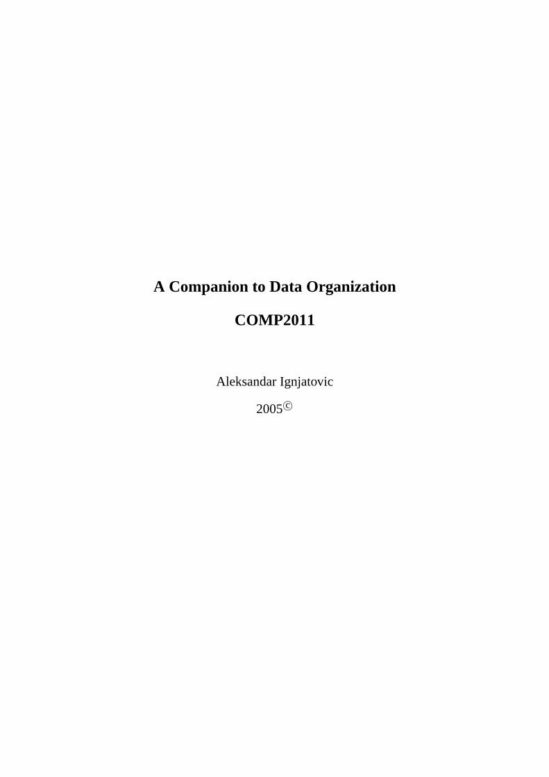
Figure 1: A medieval copy of arguably the most influential textbook ever written, Eu-clid’s Elements(Στoιχεια), from about 300 BC. It contains the oldest known algo-rithm recorded, Euclid’s algorithm for computing the Greatest Common Divisor (GCD)of two natural numbers.
Figure 2: First data structures: a Mesopotamian cuneiform tablet from about 3000 BCwith an inventory list.
Preface
This booklet is not meant to be a textbook, but only a companion to the textbook that we
use in this course, Cormen, Leiserson, Rivest and Stein’sIntroduction to Algorithms, the
second edition. Its purpose is to help you read the appropriate sections of the textbook,
and integrate it better with the rest of the course. It also adds a number of exercises not
present in the textbook.Please read the textbook and do not rely on this supplement
only.
3

Contents
1 Introduction 7
1.1 What is an Algorithm? . . . . . . . . . . . . . . . . . . . . . . . . . . 7
1.2 Abstraction Levels in Data Organization . . . . . . . . . . . . . . . . . 10
1.2.1 Abstract Data Structures . . . . . . . . . . . . . . . . . . . . . 11
1.2.2 Abstract Data Types . . . . . . . . . . . . . . . . . . . . . . . 16
1.3 Recursion . . . . . . . . . . . . . . . . . . . . . . . . . . . . . . . . . 24
1.3.1 What is Recursion? . . . . . . . . . . . . . . . . . . . . . . . . 24
1.3.2 Types of Recursion . . . . . . . . . . . . . . . . . . . . . . . . 25
1.3.3 Linear versus Divide-and-Conquer Recursion in Sorting . . . . 30
1.4 Asymptotic Time Complexity of Algorithms . . . . . . . . . . . . . . . 38
1.4.1 Basics . . . . . . . . . . . . . . . . . . . . . . . . . . . . . . . 38
1.4.2 Asymptotic growth rate of functions . . . . . . . . . . . . . . . 40
1.4.3 Basic property of logarithms . . . . . . . . . . . . . . . . . . . 42
2 Sorting Algorithms 47
2.1 The Quick Sort . . . . . . . . . . . . . . . . . . . . . . . . . . . . . . 48
2.2 Randomization . . . . . . . . . . . . . . . . . . . . . . . . . . . . . . 59
5

Chapter 1
Introduction
1.1 What is an Algorithm?
An algorithm is a collection of precisely defined steps that are executable using certain
specified mechanical methods. By “mechanical” we mean the methods that do not
involve any creativity, intuition or even intelligence. Thus, algorithms are specified by
detailed, easily repeatable “recipes”. The word “algorithm” comes by corruption of
the name ofMukhammad ibn Musa Al-Khorezmi(780-850) who wrote an important
book on algebra,“Kitab al muhtasar fi hisab al gabr w’al muqubalah”(“A compact
introduction to calculation using rules of completion and reduction”). It is also believed
that the title of this book is the source of the word “algebra”.
In this course we will deal only with algorithms that are given as sequences of
steps, thus assuming that only one step can be executed at a time. Such algorithms are
calledsequential. If the action of each step gives the same result whenever this step
is executed for the same input, we call such algorithmsdeterministic. If the execution
involves some random process, say throwing some (possibly software simulated) coin
7
8 Chapter 1. Introduction
or dice, such algorithms are calledrandomized algorithms. Randomized algorithms are
important tools for tasks that have to be repeated many times.
Example 1.1 A sorting algorithmfor an input sequence of numbers〈a1,a2, ,an〉 pro-
duces as output a permutation〈aπ(1),aπ(2), . . . ,aπ(n)〉 of the input sequence such that
aπ(1) ≤ aπ(2) ≤ . . .≤ aπ(n).
There are many algorithms that accomplish the task of sorting that have different
efficiency for different kinds of inputs. Efficiency of an algorithm is measured by its
time complexity, and toanalyzean algorithm means to determine its time complexity
for the given type of inputs. Usually we do theworse case analysis, i.e., we determine
the largest number of basic steps needed to execute the algorithm for any input of size
n. Also important is theaverage caseanalysis. It provides the expected number of
basic steps needed to execute the algorithm for inputs of length at mostn, assuming
certain probability distribution of these inputs. Thus, if we assume that all inputs of
size at mostn are equally likely, the average case analysis gives the average number of
steps needed to execute the algorithm for all inputs of size at mostn. Clearly, a time
complexity functionT(n) is non decreasing, i.e.,m≤ n⇒ T(m)≤ T(n). An algorithm
is optimal if it provides the necessary functionality with the smallest possible numbers
of steps for each input.
Another important feature of an algorithm is itscorrectnessi.e., that it provides
correct functionality for all possible inputs. Generally, the only way to ensure the cor-
rectness of an algorithm is by means of a mathematical proof. This is due to the fact
that it is impossible to test an algorithm for all possible inputs. Sometimes such cor-
rectness proofs are very simple, because the correctness follows immediately from the
1.1. What is an Algorithm? 9
definition of the algorithm. However, sometimes the correctness of an algorithm is far
from obvious and requires a meticulous proof.
The activity of designing an algorithm and an appropriate data structure for the
problem at hand is calledproblem solving. Clearly, problem solving precedes writing a
code, and in fact it is largely independent of the programming language or even of the
programming paradigm used (e.g., object oriented, imperative, etc). This is true for as
long as the algorithm is to be implemented on a standard, sequential processor. After
problem solving is completed and the correctness of designed algorithms is verified,
there is still much to do, namely one has toimplementthe algorithms and the associated
data structures in a specific programming language. Such implementation has to meet
numerous important criteria:
• reliability - the implementation is correct and it will not introduce vulnerabilities
to the system that runs it.
• maintainability - one can easily replace a part of the code in order to provide
somewhat different functionality;
• extensibility- to obtain more features, additional piece of code can be integrated
with the existing code with little or no modifications of the already existing code
needed;
• reusability - possibility of using parts of the code in another application. This is
accomplished bymodular design.
• robustness- the implementation does not crush if the user inputs an unexpected
or illegitimate input;
10 Chapter 1. Introduction
• user friendliness- users can interact with ease with the program during its exe-
cution;
• implementation time- implementation takes a reasonable amount of program-
ming time and other resources.
Note that these features are not features of algorithms and data structures, but rather,
of their implementations. Clearly, it is equally important that both the algorithms and
the data structures on one hand, as well as their implementation on the other hand, be
correct. Separation of design and implementation simplifies the process of software
development and helps ensure reliability of the final product, because it allows that the
correctness of algorithms be verified prior to their their implementations.
1.2 Abstraction Levels in Data Organization
While solving a problem that involves a collection of objects of any kind, only a limited
number of properties of these objects and a limited number of their mutual relations are
relevant for the problem considered. Thus, objects can be “abstracted away”, i.e., re-
placed with suitable “names” and with an abstract representation of their corresponding
properties and mutual relations. These properties of objects and their relations we call
data.
Data is organized in a well-defined and structured abstract entity, called adata struc-
ture. Note that this makes sense regardless of whether data is to be manipulated by a
human or by a machine. The data corresponding to each object usually consists of a
keythat identifies the object that data is abstracted from, and the remaining data that is
called thesatellite data. Together they form arecord, which is an element of the data
1.2. Abstraction Levels in Data Organization 11
structure. Data structures can change their content as elements are added or deleted,
and for that reason a data structure is adynamic set.
Example 1.2 A group of students as a “set of objects”, with data for each student con-
sisting of their names, used as the corresponding key, and their date of birth, address
and student number, organized in a data structure in the form of an alphabetical list.
1.2.1 Abstract Data Structures
We can further ignore what particular data is involved, and consider only the abstract
structure into which data is organized for the purpose of efficient storage and retrieval,
e.g., a linked list, a binary search tree, etc. In this way, we obtain anabstract data
structure (ADS). An ADS is defined by the details of its internal organization and by
internal operations that are used to maintain its properties as elements are added or
removed. Information about what kind of data will be stored in such structures is not a
part of abstract data structure specification. This has an important practical consequence
that the same abstract data structure can be used to store different type of data, say
integers or floating point numbers, by simply instantiating the same data structure with
a different particulartypeof data.
Examples of Abstract Data Structures
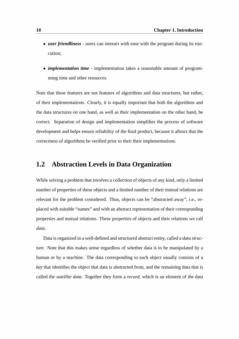
1.1 A Singly Linked List is an Abstract Data Structure organized in a list of elements
that has a special beginning element (thehead) and an end element (thetail). Further,
each element contains information what the next element in the list is.
12 Chapter 1. Introduction
head next next next tail
• • •
Figure 1.1: A singly linked list
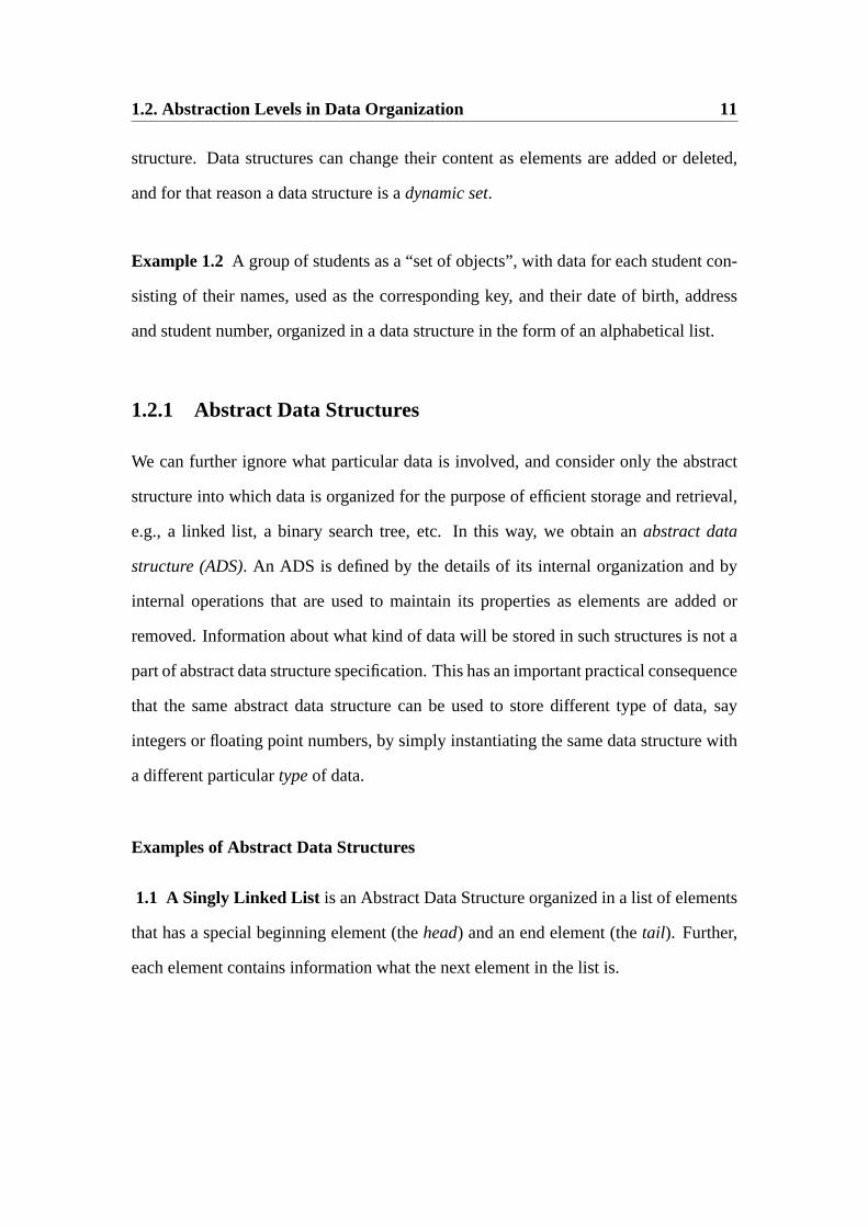
1.2 A Doubly Linked List satisfies all properties of a singly linked list, but also con-
tains with each element information what are its predecessor and its successor.
head prev. next prev next prev. next tail
• • •
Figure 1.2: A doubly linked list
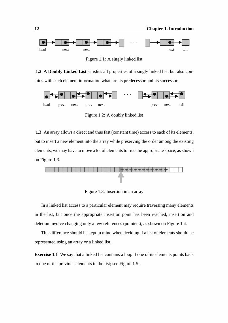
1.3 An array allows a direct and thus fast (constant time) access to each of its elements,
but to insert a new element into the array while preserving the order among the existing
elements, we may have to move a lot of elements to free the appropriate space, as shown
on Figure 1.3.
Figure 1.3: Insertion in an array
In a linked list access to a particular element may require traversing many elements
in the list, but once the appropriate insertion point has been reached, insertion and
deletion involve changing only a few references (pointers), as shown on Figure 1.4.
This difference should be kept in mind when deciding if a list of elements should be
represented using an array or a linked list.
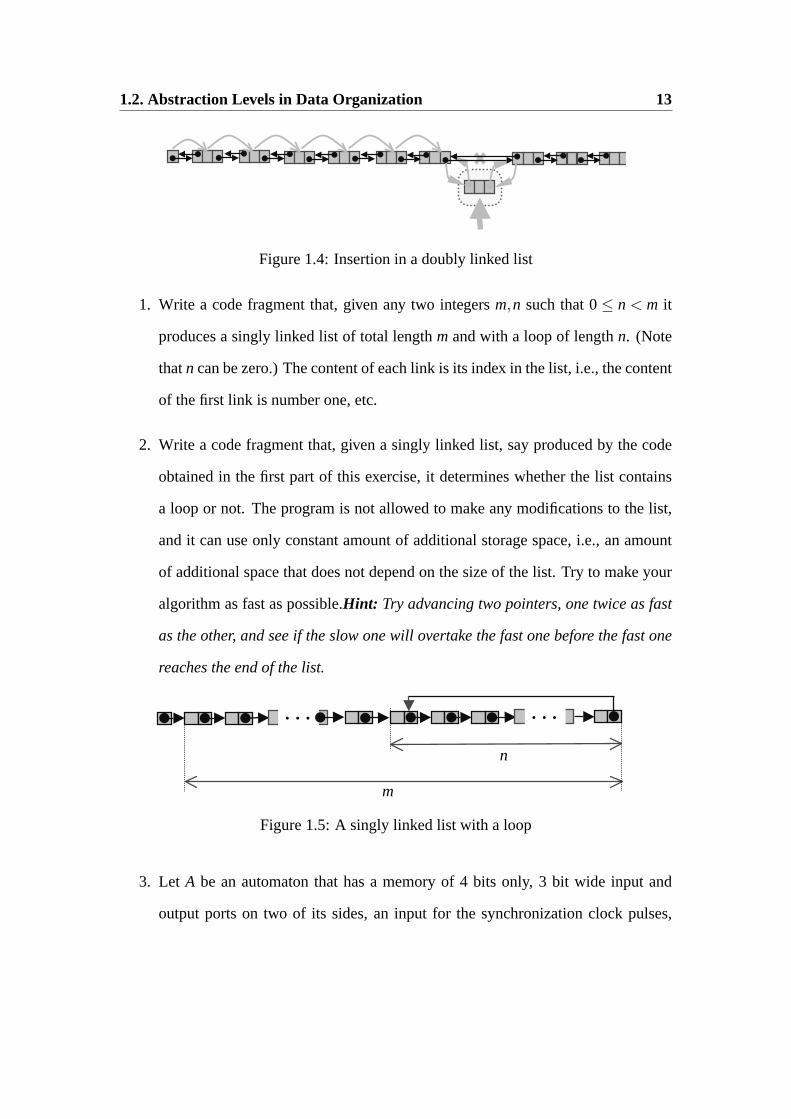
Exercise 1.1We say that a linked list contains a loop if one of its elements points back
to one of the previous elements in the list; see Figure 1.5.
1.2. Abstraction Levels in Data Organization 13
Figure 1.4: Insertion in a doubly linked list
1. Write a code fragment that, given any two integersm,n such that0≤ n < m it
produces a singly linked list of total lengthm and with a loop of lengthn. (Note
thatn can be zero.) The content of each link is its index in the list, i.e., the content
of the first link is number one, etc.
2. Write a code fragment that, given a singly linked list, say produced by the code
obtained in the first part of this exercise, it determines whether the list contains
a loop or not. The program is not allowed to make any modifications to the list,
and it can use only constant amount of additional storage space, i.e., an amount
of additional space that does not depend on the size of the list. Try to make your
algorithm as fast as possible.Hint: Try advancing two pointers, one twice as fast
as the other, and see if the slow one will overtake the fast one before the fast one
reaches the end of the list.
• • • • • •
m
n
Figure 1.5: A singly linked list with a loop
3. Let A be an automaton that has a memory of 4 bits only, 3 bit wide input and
output ports on two of its sides, an input for the synchronization clock pulses,
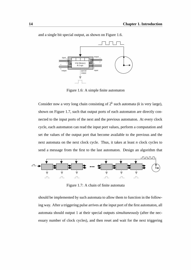
14 Chapter 1. Introduction
and a single bit special output, as shown on Figure 1.6.
output
input output
output
input
special output
input
4 bit Memory & Logic
Figure 1.6: A simple finite automaton
Consider now a very long chain consisting of2k such automata (k is very large),
shown on Figure 1.7, such that output ports of each automaton are directly con-
nected to the input ports of the next and the previous automaton. At every clock
cycle, each automaton can read the input port values, perform a computation and
set the values of the output port that become available to the previous and the
next automata on the next clock cycle. Thus, it takes at leastn clock cycles to
send a message from the first to the last automaton. Design an algorithm that
Figure 1.7: A chain of finite automata
should be implemented by such automata to allow them to function in the follow-
ing way. After a triggering pulse arrives at the input port of the first automaton, all
automata should output 1 at their special outputssimultaneously(after the nec-
essary number of clock cycles), and then reset and wait for the next triggering
1.2. Abstraction Levels in Data Organization 15
pulse. Notice that, given extreme memory limitations of these finite automata,
they cannot determine their position in the chain.Hint: You might find the hint
for 2. above inspiring!
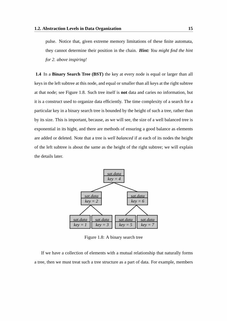
1.4 In a Binary Search Tree (BST) the key at every node is equal or larger than all
keys in the left subtree at this node, and equal or smaller than all keys at the right subtree
at that node; see Figure 1.8. Such tree itself isnot data and caries no information, but
it is a construct used to organize data efficiently. The time complexity of a search for a
particular key in a binary search tree is bounded by the height of such a tree, rather than
by its size. This is important, because, as we will see, the size of a well balanced tree is
exponential in its hight, and there are methods of ensuring a good balance as elements
are added or deleted. Note that a tree iswell balancedif at each of its nodes the height
of the left subtree is about the same as the height of the right subtree; we will explain
the details later.
sat.data key = 6
sat.data key = 2
sat.data key = 7
sat.data key = 5
sat.data key = 4
sat.data key = 1
sat.data key = 3
Figure 1.8: A binary search tree
If we have a collection of elements with a mutual relationship that naturally forms
a tree, then we must treat such a tree structure as a part of data. For example, members
16 Chapter 1. Introduction
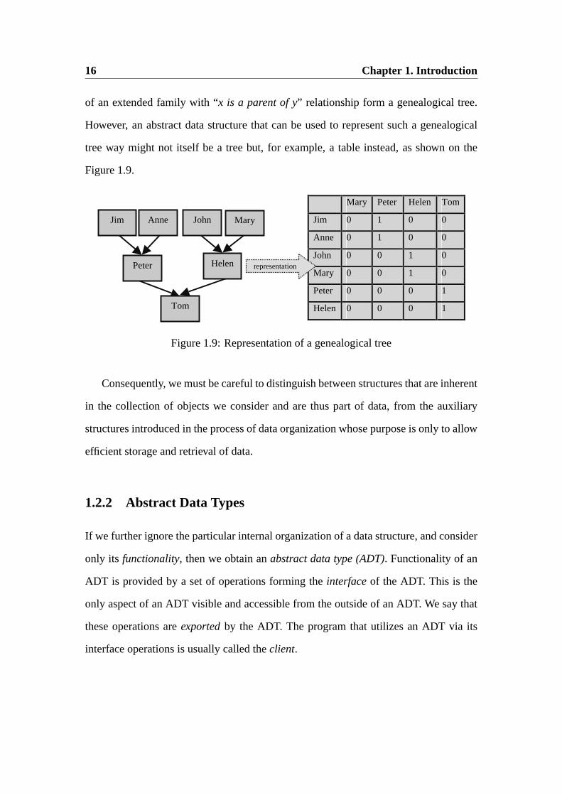
of an extended family with “x is a parent of y” relationship form a genealogical tree.
However, an abstract data structure that can be used to represent such a genealogical
tree way might not itself be a tree but, for example, a table instead, as shown on the
Figure 1.9.
Mary Peter Helen Tom
Jim 0 1 0 0
Anne 0 1 0 0
John 0 0 1 0
Mary 0 0 1 0
Peter 0 0 0 1
Helen 0 0 0 1
Peter Helen
Jim Anne John Mary
representation
Tom
Figure 1.9: Representation of a genealogical tree
Consequently, we must be careful to distinguish between structures that are inherent
in the collection of objects we consider and are thus part of data, from the auxiliary
structures introduced in the process of data organization whose purpose is only to allow
efficient storage and retrieval of data.
1.2.2 Abstract Data Types
If we further ignore the particular internal organization of a data structure, and consider
only its functionality, then we obtain anabstract data type (ADT). Functionality of an
ADT is provided by a set of operations forming theinterfaceof the ADT. This is the
only aspect of an ADT visible and accessible from the outside of an ADT. We say that
these operations areexportedby the ADT. The program that utilizes an ADT via its
interface operations is usually called theclient.
1.2. Abstraction Levels in Data Organization 17
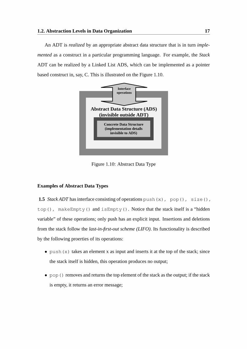
An ADT is realizedby an appropriate abstract data structure that is in turnimple-
mentedas a construct in a particular programming language. For example, theStack
ADT can be realized by a Linked List ADS, which can be implemented as a pointer
based construct in, say, C. This is illustrated on the Figure 1.10.
Interface operations
Concrete Data Structure (implementation details
invisible to ADS)
Abstract Data Structure (ADS) (invisible outside ADT)
Figure 1.10: Abstract Data Type
Examples of Abstract Data Types
1.5 Stack ADThas interface consisting of operationspush(x), pop(), size(),
top(), makeEmpty() and isEmpty() . Notice that the stack itself is a “hidden
variable” of these operations; only push has an explicit input. Insertions and deletions
from the stack follow thelast-in-first-out scheme (LIFO). Its functionality is described
by the following proerties of its operations:
• push(x) takes an element x as input and inserts it at the top of the stack; since
the stack itself is hidden, this operation produces no output;
• pop() removes and returns the top element of the stack as the output; if the stack
is empty, it returns an error message;
18 Chapter 1. Introduction
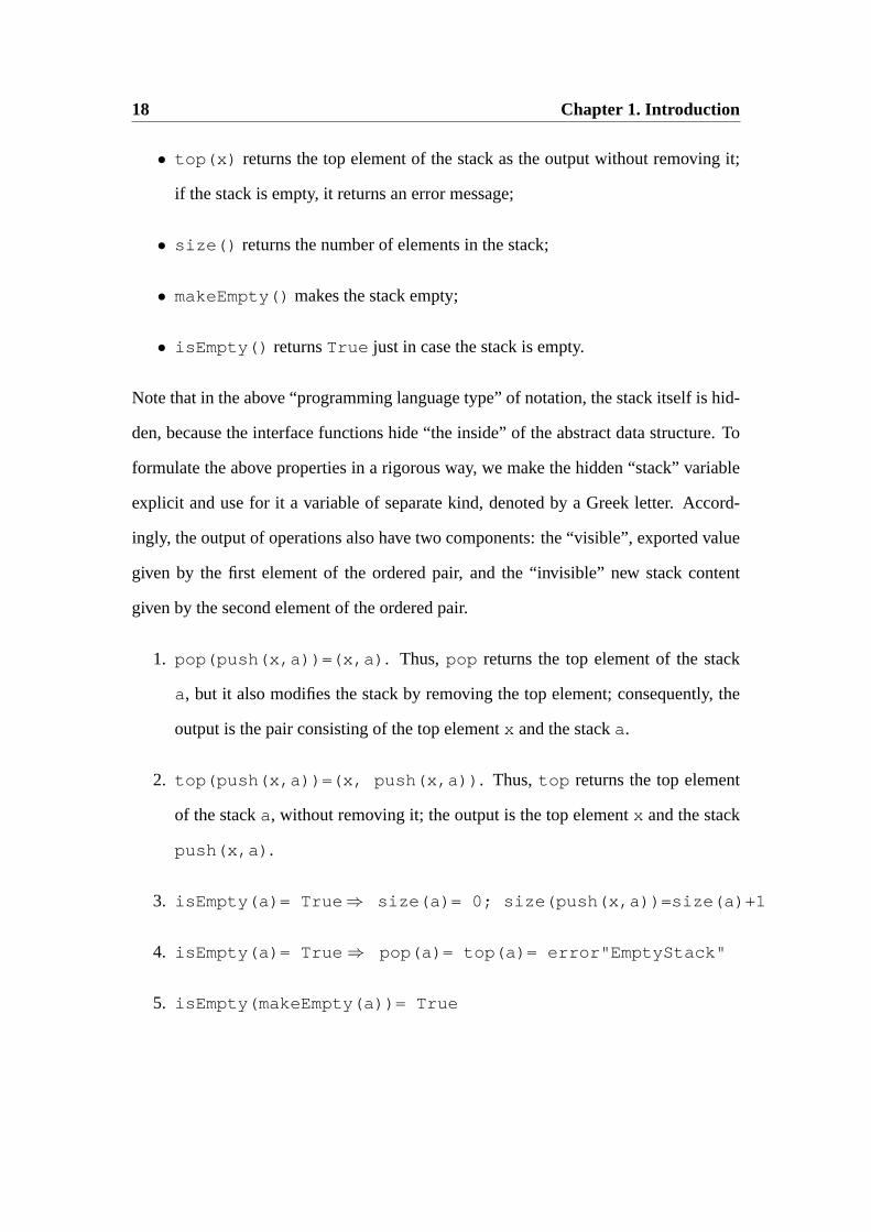
• top(x) returns the top element of the stack as the output without removing it;
if the stack is empty, it returns an error message;
• size() returns the number of elements in the stack;
• makeEmpty() makes the stack empty;
• isEmpty() returnsTrue just in case the stack is empty.
Note that in the above “programming language type” of notation, the stack itself is hid-
den, because the interface functions hide “the inside” of the abstract data structure. To
formulate the above properties in a rigorous way, we make the hidden “stack” variable
explicit and use for it a variable of separate kind, denoted by a Greek letter. Accord-
ingly, the output of operations also have two components: the “visible”, exported value
given by the first element of the ordered pair, and the “invisible” new stack content
given by the second element of the ordered pair.
1. pop(push(x,a))=(x,a) . Thus,pop returns the top element of the stack
a, but it also modifies the stack by removing the top element; consequently, the
output is the pair consisting of the top elementx and the stacka.
2. top(push(x,a))=(x, push(x,a)) . Thus,top returns the top element
of the stacka, without removing it; the output is the top elementx and the stack
push(x,a) .
3. isEmpty(a)= True ⇒ size(a)= 0; size(push(x,a))=size(a)+1
4. isEmpty(a)= True ⇒ pop(a)= top(a)= error"EmptyStack"
5. isEmpty(makeEmpty(a))= True
1.2. Abstraction Levels in Data Organization 19
The functionality of the queue is thus defined purely algebraically. This highlights
the fact that an ADT is defined only by its functionality, completely hiding how such
functionality is achieved. There are important practical benefits of such an approach:
1. It eliminates the need to maintain uniform data representation throughout the sys-
tem: for as long as we know how interface operations input and output data, inside
an ADT data can be represented in an arbitrary way, different from the way how
the same data is represented in the client program. Thus, changes in the design of
the client or the ADT raise no question regarding their subsequent compatibility.
2. Design becomes modular; different modules can be designed by different people,
who need to know nothing about how other modules are designed, but only what
the interface operations are and what the functionality provided by the ADT is.
3. The structure of the system can be described on a higher level, without going into
the details of implementation. This greatly simplifies design and understanding
of complex systems. It also simplifies testing and verification of systems, because
each module can be tested separately prior to its incorporation into the system.
4. Modules can be easily reused in other systems without change for as long as the
functionality needed is the same.
Examples of stack applications include: history of pages visited in a Web browser; undo
sequence in a text editor; CPU stack that handles recursion; etc.
Exercise 1.2
1. Consider algebraic expressions built using the following rules:
20 Chapter 1. Introduction
(a) a variable denoted by a small Roman letter is an expression. For example,x
andy are both expressions;
(b) if t1 andt2 are expressions, then so is(t1t2);
(c) expressions can be built only using the above two rules.
Thus, for example((xy)z)w) is a correct expression (we do not remove the outer-
most parentheses), but, for example,(xy)(z is not a correct expression. Similarly,
((xy)) is not a correct expression, because it cannot be obtained using the above
rules. Design an algorithm that checks if a sequence of variables and brackets is
a correct algebraic expression or not, i.e., if it has correctly matched parenthe-
ses. Implement your procedure and test it.Hint: Set a counter and increment
it whenever you open a bracket and decrement it when you close it. Ignore the
variables.
The other most commonly used ADT is thequeue. Unlike the stack that follows
the LIFO scheme, insertions and deletions from the queue follow thefirst-in-first-out
scheme (LIFO)as shown on the Figure below.
1.6 Queue ADThas interface consisting of operationsenqueue(x), dequeue(),
front(), size(), makeEmpty() and isEmpty() . Again, the stack itself is
a “hidden variable” of these operations; onlypush has an explicit input. Since inser-
tions and deletions from the queue follow thefirst-in-first-out scheme (FIFO), a queue
encodes temporal order how elements have been added. Its functionality is specified by
the following properties of its operations:
• enqueue(x) takes an elementx as input and inserts it at the end of the queue;
since the queue itself is hidden, this operation produces no output;
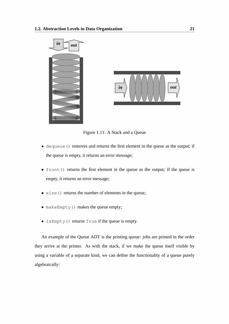
1.2. Abstraction Levels in Data Organization 21
in out
in out
Figure 1.11: A Stack and a Queue
• dequeue() removes and returns the first element in the queue as the output; if
the queue is empty, it returns an error message;
• front() returns the first element in the queue as the output; if the queue is
empty, it returns an error message;
• size() returns the number of elements in the queue;
• makeEmpty() makes the queue empty;
• isEmpty() returnsTrue if the queue is empty.
An example of the Queue ADT is the printing queue: jobs are printed in the order
they arrive at the printer. As with the stack, if we make the queue itself visible by
using a variable of a separate kind, we can define the functionality of a queue purely
algebraically:
22 Chapter 1. Introduction
1. isEmpty(a)=True ⇒ decueue(a)=front(a)=error"EmptyQueue"
2. isEmpty(a)=True ⇒ decueue(enqueue(x,a))=(x,a)
3. isEmpty(a)=True ⇒ front((enqueue(x,a)))=(x,enqueue(x,a))
4. isEmpty(a)=False ⇒ decueue(enqueue(x,a))=decueue(a)
5. isEmpty(a)=False ⇒ front(enqueue(x,a))=front(a)
6. isEmpty(a)=True ⇒ size(a)=0
7. size(enqueue(x,a))=size(a)+1
8. isEmpty(makeEmpty(a))=True
Exercise 1.3A simple implementation of a queue would consist of an array together
with two pointers that keep track of where the front and the rear end of the queue are.
However, with such a design, as elements are added and removed, the content of the
queue would move through the array and would eventually “run away” (overflow the
array) even if there are fewer elements in the queue than the size of the array. Solve this
problem by designing a circular structure. Implement it and test it.
1.7 Binary Search Tree (BST)is an ADT for efficient storage, removal and retrieval of
records(k,a) with keys that are linearly ordered. There are several versions of BST;
we chose one with the following interface operations:
• insert((k,x)) inserts element(k,x) into the BST; if there is already an
element(k,y) with the same keyk , it is replaced with the new element;
• delete(k) deletes the element with the keyk from the BST; if there is no such
element, it leaves the tree unchanged.
1.2. Abstraction Levels in Data Organization 23
• find(k) finds and outputs the element with keyk if there is such element in
the BST and it returns an error message if there is no such element;
• in(k ) returns True just in case the BST contains an element with the keyk .
• size() returns the number of elements in the BST;
• isEmpty() returns True if the BST is empty.
• makeEmpty() makes the BST empty.
• We require that all of the above operations run in time bounded byK lg(n+ 2)
whereK is a fixed constant,n is the number of elements in the tree, andlg n =
log2n.
Thus, a purely algebraic definition of a Binary Search Tree ADT is expected to be more
complicated than the definitions of a stack or a queue, because it involves not only the
interface operations but also their complexity constraints. Informally speaking, such
complexity constraints are met by requiring that a search in a BST that is obtained by
joining two trees of equal size takes only a constant number of steps more than the
search in one of them. We postpone the details until a later, systematic treatment of
BST.
Note that in the definition of BST there is no reference to any kind of tree structure,
but only to the properties of the interface operations. Their name comes from the fact
that they are in fact realized using abstract data structures that do have a tree structure.
Examples include AVL trees and Red-Black trees. Clearly, unlike stacks and queues, a
BST does not encode the order in which elements are added to the structure, but instead,
it allows retrieval of a record by the value of its key.
24 Chapter 1. Introduction
1.3 Recursion
1.3.1 What is Recursion?
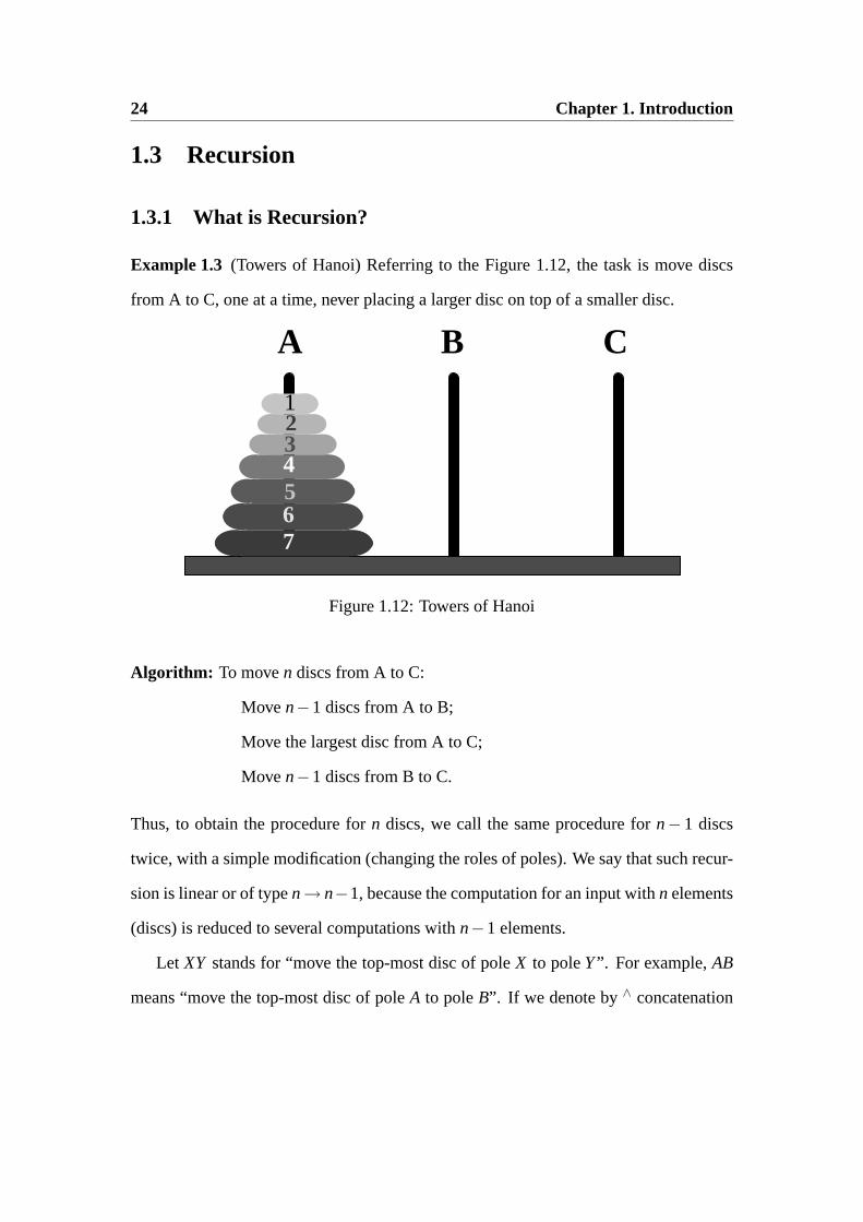
Example 1.3 (Towers of Hanoi) Referring to the Figure 1.12, the task is move discs
from A to C, one at a time, never placing a larger disc on top of a smaller disc.
A B C
1 2 3 4 5 6 7
Figure 1.12: Towers of Hanoi
Algorithm: To moven discs from A to C:
Moven−1 discs from A to B;
Move the largest disc from A to C;
Moven−1 discs from B to C.
Thus, to obtain the procedure forn discs, we call the same procedure forn−1 discs
twice, with a simple modification (changing the roles of poles). We say that such recur-
sion is linear or of typen→ n−1, because the computation for an input withn elements
(discs) is reduced to several computations withn−1 elements.
Let XY stands for “move the top-most disc of poleX to poleY”. For example,AB
means “move the top-most disc of poleA to poleB”. If we denote by∧ concatenation
1.3. Recursion 25
of moves, then the above algorithm can be written as:
f (n,A,B,C) = f (n−1,A,C,B)∧AC∧ f (n−1,B,A,C)
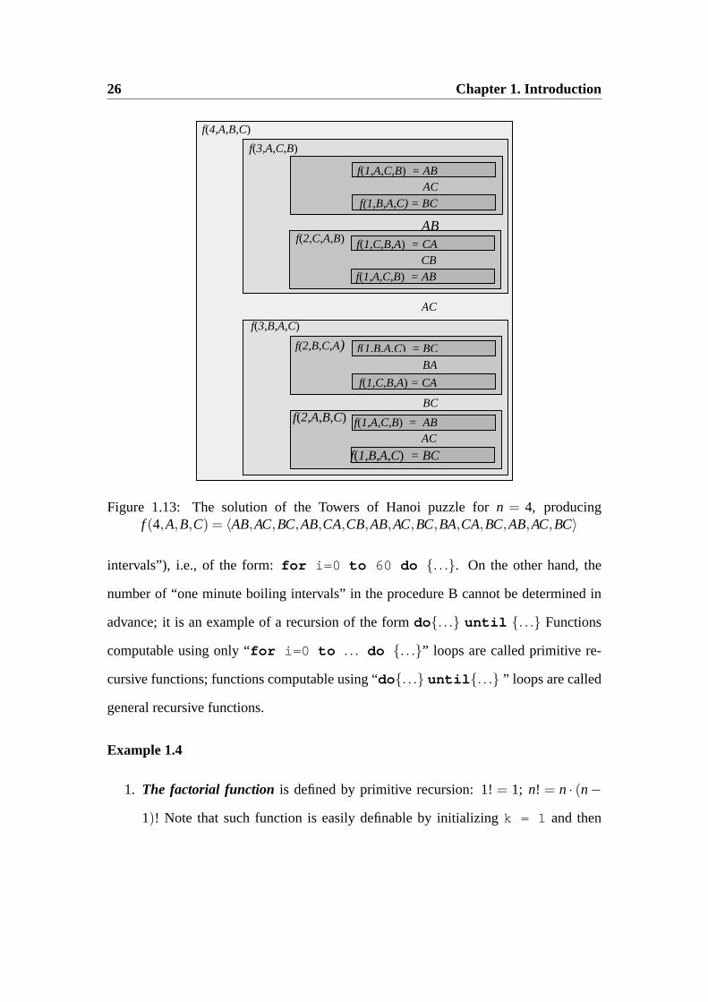
For n = 4 we can “unwind” the recursion as in the Figure 1.13 below. The boxes
correspond to recursive calls. Note that computations in each box can be completed
only after the computations in the smaller boxes contained within are completed.
Exercise 1.4Tom and his wife Mary went to a party where nine more couples were
present. Not every one knew every everyone else, so people who did not know each
other introduced themselves and shook hands. People that knew each other from before
did not shake hands. Later that evening Tom got bored, so he walked around and asked
all other guests (including his wife) how many hands they had shaken that evening, and
got 19 different answers. How many hands did Mary shake?
Hint: Try recursion on the number of couples, by finding what couple you should elim-
inate first. If there are 19 different answers what could they be? Which ones are the
most interesting numbers among those 19 numbers and how are these people related?
1.3.2 Types of Recursion
Consider the following two recipes to how to cook potatoes:
“Take a kilo of potatoes and boil them for sixty minutes.”
“Take a kilo of potatoes and boil them until soft.”
These two recipes exemplify the first major distinction among recursion types. Type
A is an example of a recursive procedure that involves a number of steps that can be
determined before the procedure has started (“keep boiling potatoes for 60 one minute
26 Chapter 1. Introduction
AC
f(2,C,A,B)
AC
f(2,B,C,A) BA
f(2,A,B,C)
AC
CB
f(1,B,A,C) = BC
f(4,A,B,C)
f(3,A,C,B)
f(3,B,A,C)
f(1,A,C,B) = AB
f(1,A,C,B) = AB
f(1,C,B,A) = CA
f(1,B,A,C) = BC
f(1,C,B,A) = CA
f(1,A,C,B) = AB
f(1,B,A,C) = BC
BC
AB
Figure 1.13: The solution of the Towers of Hanoi puzzle forn = 4, producingf (4,A,B,C) = 〈AB,AC,BC,AB,CA,CB,AB,AC,BC,BA,CA,BC,AB,AC,BC〉
intervals”), i.e., of the form:for i=0 to 60 do . . .. On the other hand, the
number of “one minute boiling intervals” in the procedure B cannot be determined in
advance; it is an example of a recursion of the formdo. . . until . . . Functions
computable using only “for i=0 to . . . do . . .” loops are called primitive re-
cursive functions; functions computable using “do. . . until . . . ” loops are called
general recursive functions.
Example 1.4
1. The factorial function is defined by primitive recursion:1! = 1; n! = n · (n−1)! Note that such function is easily definable by initializingk = 1 and then
1.3. Recursion 27
executing the loopfor i = 1 to n do k ← k · i .
2. f(n) = n th number p such that both p and p+2 are prime .
To get such a number we initializek=0, p=2 and then execute:do if p
and (p+2) are prime then k←k+1 ; p ←p+1 until k==n .
In fact, we do not even know if for everyn our algorithm will terminate. The hy-
pothesis that there infinitely many primesp such thatp+ 2 is also a prime is
known thetwin primes hypothesis.
There are functions that are not primitive recursive, yet they are still simpler than most
general recursive functions. The best known example is the Ackerman function defined
by double recursion:
F(0,n) = n+1
F(m,0) = F(m−1,1)
F(m,n) = F(m−1,F(m,n−1)) for m, n > 0
One can show that such function cannot be reduced to the usual primitive recursion; in
fact, Ackerman function grows faster than any function defined by primitive recursion.
Exercise 1.5Write a program that computesF(m,n) and try to evaluateF(3,3) and
F(4,4).
In this booklet we call a harder exercise aproblem; nevertheless, you should not be
discouraged; try to solve it!
Problem 1.1 Two thieves have robbed a warehouse and have to split a pile of items
without price tags on them. How do they do this in away that ensures that each thief
28 Chapter 1. Introduction
believesthat he has got at least one half of the value of the whole pile?(You might want
to try to solve this problem before reading any further.)The solution is that one of the
two thieves splits the pile in two parts, so that he believes that both parts are of equal
value. The other thief then chooses the part that he believes is at least one half. Assume
now that ten thieves have robbed a warehouse. How do they split the pile of items so
that each thief believes that he got at least one tenth of the total value of the pile?
Linear Recursion considered above (except the double recursion used to define the
Ackerman function) reduces computation ofF(n,x) to one or several computations
of F(n−1, . . .). For example, identityn! = n(n−1)! reduces computation ofn! to a
computation of(n− 1)! and a multiplication of the result byn. Much more efficient
is divide-and-conquer recursion, that reduces a computation ofF(n,x) to computations
of F(dn/ke, . . .), wherek > 1. Oftenk = 2, and soF(n, . . .) is reduced to computations
of the formF(dn/2e, . . .). We sometimes do not write integer part function and simply
write F(n/2, . . .) for F(dn/2e, . . .), if no confusion can arise.
Example 1.5 y= xn can be computed using linear recursion as follows:x0 = 1; xn+1 =
x · xn. However, one can also use recursion as follows:x0 = 1; x2n = (xn)2; x2n+1 =
x · (xn)2. Clearly, this way the number of multiplications needed to evaluatexn is at
most2 lg n.
Example 1.6 We are given 27 coins of the same denomination; we know that one of
them is counterfeit and that it is lighter than the others. Find the counterfeit coin by
weighing coins on a pan balance only three times.
Solution: Split 27 = 33 coins into three equal groups with 9 coins each. Put two
groups on the pan balance. If equal, the false coin must be in the third group; otherwise
1.3. Recursion 29
take the lighter group. Split these nine coins into three groups with three coins each and
compare two of these groups. As in the previous step, you can find a group containing
the false coin. Finally, compare two of the three coins left; if equal, the false coin is the
remaining coin, otherwise take the coin on the lighter side. 2
Notice that if we had3n coins and can weigh coins n times, then splitting them into
three groups with3(n−1) coins each and comparing two of the three groups we end up
with 3(n−1) coins where the fake coin might be and can weighn−1 times. Thus, this
type of recursion reduces the size of the problem into a sub-problem of size equal to a
fraction of the original problem; this is why such recursion is called divide-and-conquer
recursion.
Exercise 1.6We are given twelve coins and one of them is a counterfeit but we do not
know if it is heavier or lighter. Determine which one is a counterfeit and if it is lighter
or heavier by weighing coins on a pan balance three times only.
Hint: divide and conquer; note that you can reuse coins that are established not to be
counterfeit!
Example 1.7 We have nine coins and three of them are heavier than the remaining six.
Can you find the heavier coins by weighing coins on a pan balance only four times?
Solution: If we weigh the coins four times, since every weighing has three possi-
ble outcomes, we have altogether34 = 81 outcomes altogether. However, there are(9
3
)= 9·8·7
3! = 84 possible combinations what three coins out of nine might be heavier.
Thus, the number of possibilities we have do distinguish between is larger than the
number of possible outcomes of our weighing! Consequently, it is not possible to find
30 Chapter 1. Introduction
the heavier coins by weighing coins on a pan balance only four times. 2
This is an example of the lower bound estimation for the complexity of algorithms,
i.e., estimation of the minimal number of steps needed to solve a problem for an input
of given size. Exactly the same method as above can be used to determine the minimal
number of steps needed to sort a sequence of numbers by comparing pairs of numbers.
1.3.3 Linear versus Divide-and-Conquer Recursion in Sorting
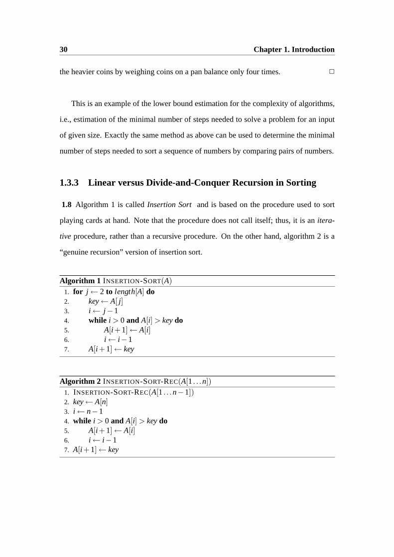
1.8 Algorithm 1 is calledInsertion Sort and is based on the procedure used to sort
playing cards at hand. Note that the procedure does not call itself; thus, it is anitera-
tive procedure, rather than a recursive procedure. On the other hand, algorithm 2 is a
“genuine recursion” version of insertion sort.
Algorithm 1 INSERTION-SORT(A)1. for j ← 2 to length[A] do2. key← A[ j]3. i ← j−14. while i > 0 and A[i] > keydo5. A[i +1]← A[i]6. i ← i−17. A[i +1]← key
Algorithm 2 INSERTION-SORT-REC(A[1. . .n])1. INSERTION-SORT-REC(A[1. . .n−1])2. key← A[n]3. i ← n−14. while i > 0 and A[i] > keydo5. A[i +1]← A[i]6. i ← i−17. A[i +1]← key
1.3. Recursion 31
key
already sorted
key > key jth
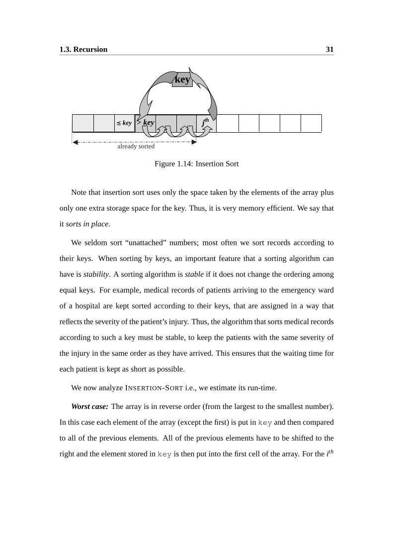
Figure 1.14: Insertion Sort
Note that insertion sort uses only the space taken by the elements of the array plus
only one extra storage space for the key. Thus, it is very memory efficient. We say that
it sorts in place.
We seldom sort “unattached” numbers; most often we sort records according to
their keys. When sorting by keys, an important feature that a sorting algorithm can
have isstability. A sorting algorithm isstableif it does not change the ordering among
equal keys. For example, medical records of patients arriving to the emergency ward
of a hospital are kept sorted according to their keys, that are assigned in a way that
reflects the severity of the patient’s injury. Thus, the algorithm that sorts medical records
according to such a key must be stable, to keep the patients with the same severity of
the injury in the same order as they have arrived. This ensures that the waiting time for
each patient is kept as short as possible.
We now analyzeINSERTION-SORT i.e., we estimate its run-time.
Worst case:The array is in reverse order (from the largest to the smallest number).
In this case each element of the array (except the first) is put inkey and then compared
to all of the previous elements. All of the previous elements have to be shifted to the
right and the element stored inkey is then put into the first cell of the array. For theith
32 Chapter 1. Introduction
element this takesci many steps. The constantc depends on what exactly elementary
instructions that can be executed in a single step are. Thus the total number of steps is
a quadratic polynomial inn:
n
∑i=2
ci = c
(n(n−1)
2−1
)= c
n2 +n−22
(1.1)
We did not count overhead of invoking subroutines etc. However, this overhead is linear
in n (i.e., a constant multiple ofn) and thus it does not change the nature of the estimate
of the time complexity of the entire algorithm, which remains quadratic inn. We will
develop later a calculus (the “O-notation”) that will allow us to estimate the growth rate
of functions without having to worry about such “details”.
Average case:If the numbers in the array are randomly chosen, any member of the
array is smaller than about one half of the previous elements of the array. Thus, for the
ith element in the array there will be abouti/2 comparisons and shifts. Consequently,
the total number of operations will be about
n
∑i=2
ci2
=c2
n2 +n−22
(1.2)
i.e., it is again a quadratic polynomial inn. Thus, the average case is about as bad as
the worst case. If you have to sort many arrays with randomly distributed content, the
algorithm will on average run in quadratic time in the length of the arrays. This, as we
will see, is very slow.
Best case:The array is already sorted. In this case each element of the array (except
the first) is put in key and then, after a comparison with the previous element, it is
returned to its old position. Thus, for each element of the array the number of atomic
1.3. Recursion 33
operations (moving numbers, comparing numbers) is constant. Consequently the total
number of operations is of the formcn, i.e. it is linear inn.
What is wrong with the above “analysis”?There isno such thing as “the best
case analysis”. The “best case” provides no useful information. However, knowing a
significant class of inputs for which an algorithm is particularly fast can be useful. For
example, if you expect few inversions in your input sequences, thenINSERTION SORT
algorithm will run in linear time, which is very fast. This happens if you sort checks
in a bank: most of the checks arrive to the bank in the order you write them, with few
inversions.
Exercise 1.7Let k be a natural number. Consider the familyAk of all arraysA[1. . .n]
such that for everyi ≤ n there are at mostk elements amongA[1. . . i−1] larger than
A[i]. Show that there exists a constantc such that every arrayA[1. . .n] from Ak can be
sorted in timec·n.
Exercise 1.8 Insertion sort consists of two main operations: searching for the right
place in the list where the key should be inserted, and inserting the key element into the
list. If the list of elements is realized as an array, what operation is the bottle-neck that
accounts for the quadratic run time of the Insertion Sort? What if the list is implemented
as a linked list? Refer to the remark 1.3 on page 12.
Divide-and-Conquer Recursionconsists of three steps at each level of recursion:
• Divide the problem into a number of sub-problems of smaller size.
• Conquerthe sub-problems using recursive calls. If the problem size is very small,
i.e., at the base of recursion, do it directly without using a recursion call.
34 Chapter 1. Introduction
• Combine the solutions of the sub-problems into a solution of the starting prob-
lem.
MERGE-SORT(A, p, r) sorts the elements of the sequence contained in the sub-array
A[p. . . r] of an arrayA in the following way. It:
• divides the n-element sequence into two subsequences of sizedn/2e andbn/2c;
• conquers by sorting the two subsequences using recursive calls of Merge-Sort.
• merges the two sorted subsequences to get the initial sequence sorted.
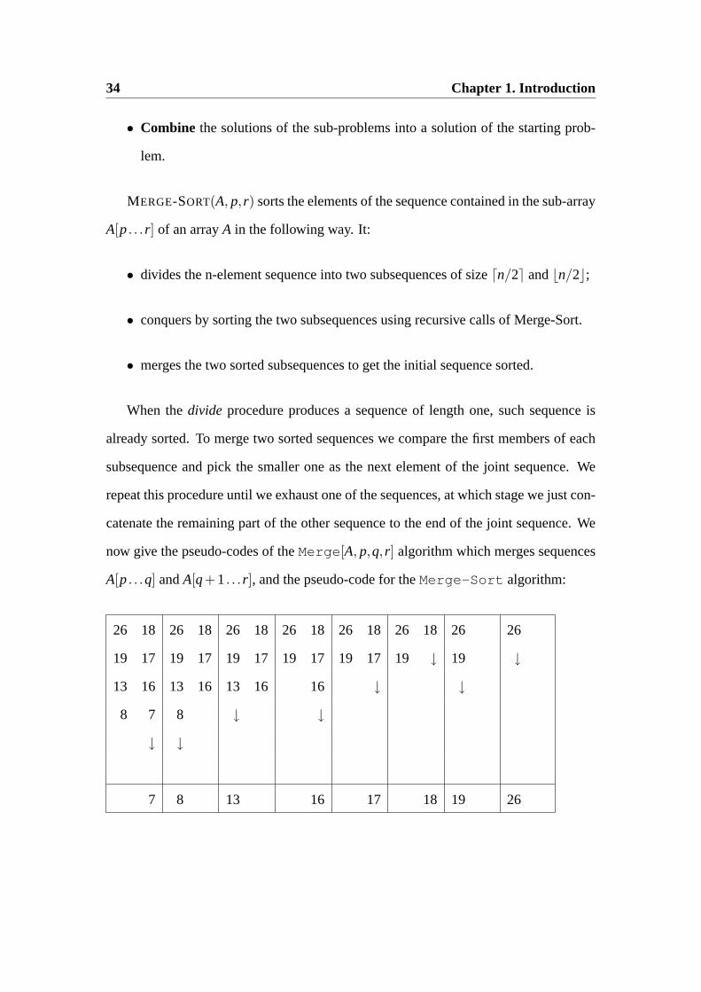
When thedivide procedure produces a sequence of length one, such sequence is
already sorted. To merge two sorted sequences we compare the first members of each
subsequence and pick the smaller one as the next element of the joint sequence. We
repeat this procedure until we exhaust one of the sequences, at which stage we just con-
catenate the remaining part of the other sequence to the end of the joint sequence. We
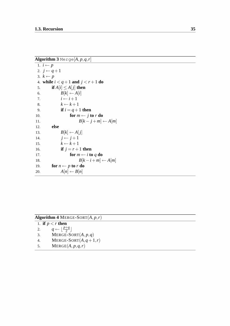
now give the pseudo-codes of theMerge [A, p,q, r] algorithm which merges sequences
A[p. . .q] andA[q+1. . . r], and the pseudo-code for theMerge-Sort algorithm:
26 18 26 18 26 18 26 18 26 18 26 18 26 26
19 17 19 17 19 17 19 17 19 17 19 ↓ 19 ↓13 16 13 16 13 16 16 ↓ ↓8 7 8 ↓ ↓
↓ ↓
7 8 13 16 17 18 19 26
1.3. Recursion 35
Algorithm 3 Merge [A, p,q, r]1. i ← p2. j ← q+13. k← p4. while i < q+1 and j < r +1 do5. if A[i]≤ A[ j] then6. B[k]← A[i]7. i ← i +18. k← k+19. if i = q+1 then
10. for m← j to r do11. B[k− j +m]← A[m]12. else13. B[k]← A[ j]14. j ← j +115. k← k+116. if j = r +1 then17. for m← i to q do18. B[k− i +m]← A[m]19. for n← p to r do20. A[n]← B[n]
Algorithm 4 MERGE-SORT(A, p, r)1. if p < r then2. q← b p+q
2 c3. MERGE-SORT(A, p,q)4. MERGE-SORT(A,q+1, r)5. MERGE(A, p,q, r)
36 Chapter 1. Introduction
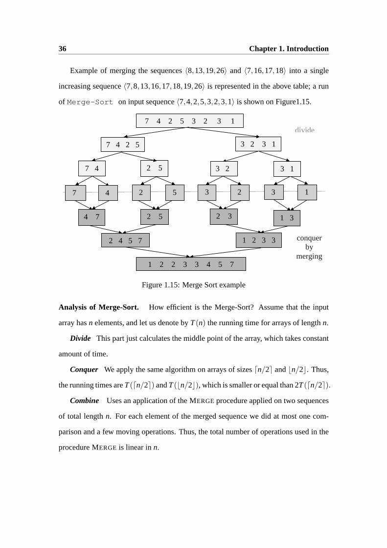
Example of merging the sequences〈8,13,19,26〉 and 〈7,16,17,18〉 into a single
increasing sequence〈7,8,13,16,17,18,19,26〉 is represented in the above table; a run
of Merge-Sort on input sequence〈7,4,2,5,3,2,3,1〉 is shown on Figure1.15.
divide
conquer by
merging
7 4 2 5 3 2 3 1
7 4 2 5 3 2 3 1
3 2 3 1 7 4 2 5
7 4 2 5 3 1 3 2
4 7 2 5 2 3 1 3
2 4 5 7 1 2 3 3
1 2 2 3 3 4 5 7
Figure 1.15: Merge Sort example
Analysis of Merge-Sort. How efficient is the Merge-Sort? Assume that the input
array hasn elements, and let us denote byT(n) the running time for arrays of lengthn.
Divide This part just calculates the middle point of the array, which takes constant
amount of time.
Conquer We apply the same algorithm on arrays of sizesdn/2e andbn/2c. Thus,
the running times areT(dn/2e) andT(bn/2c), which is smaller or equal than2T(dn/2e).Combine Uses an application of theMERGEprocedure applied on two sequences
of total lengthn. For each element of the merged sequence we did at most one com-
parison and a few moving operations. Thus, the total number of operations used in the
procedureMERGE is linear inn.
1.3. Recursion 37
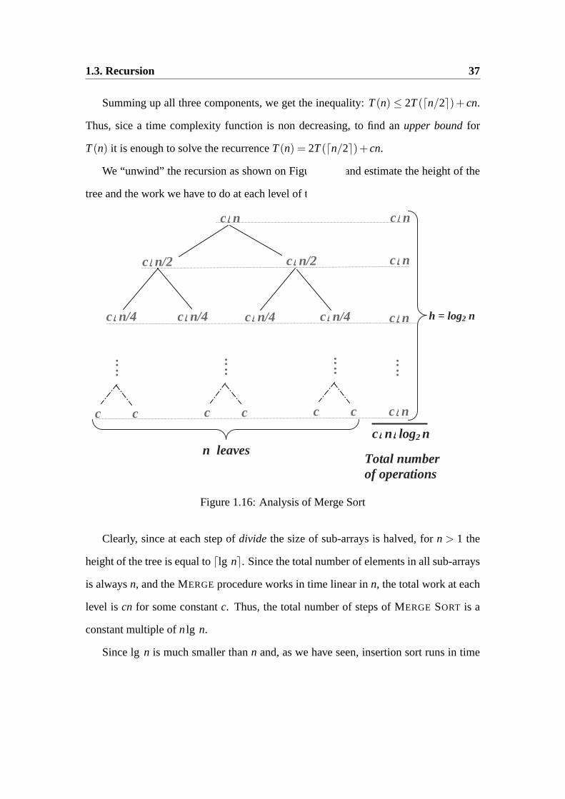
Summing up all three components, we get the inequality:T(n) ≤ 2T(dn/2e)+cn.
Thus, sice a time complexity function is non decreasing, to find anupper boundfor
T(n) it is enough to solve the recurrenceT(n) = 2T(dn/2e)+cn.
We “unwind” the recursion as shown on Figure 1.16 and estimate the height of the
tree and the work we have to do at each level of the tree.
h = log2 n
c⋅⋅⋅⋅ n
c⋅⋅⋅⋅ n/2 c⋅⋅⋅⋅ n/2
c⋅⋅⋅⋅ n/4 c⋅⋅⋅⋅ n/4 c⋅⋅⋅⋅ n/4
c⋅⋅⋅⋅ n
c⋅⋅⋅⋅ n
c⋅⋅⋅⋅ n
c⋅⋅⋅⋅ n
c⋅⋅⋅⋅ n⋅⋅⋅⋅ log2 n n leaves
c c
: :
: :
Total number of operations
c c
: :
c c
: :
c⋅⋅⋅⋅ n/4
Figure 1.16: Analysis of Merge Sort
Clearly, since at each step ofdivide the size of sub-arrays is halved, forn > 1 the
height of the tree is equal todlg ne. Since the total number of elements in all sub-arrays
is alwaysn, and theMERGEprocedure works in time linear inn, the total work at each
level iscn for some constantc. Thus, the total number of steps ofMERGE SORT is a
constant multiple ofnlg n.
Sincelg n is much smaller thann and, as we have seen, insertion sort runs in time
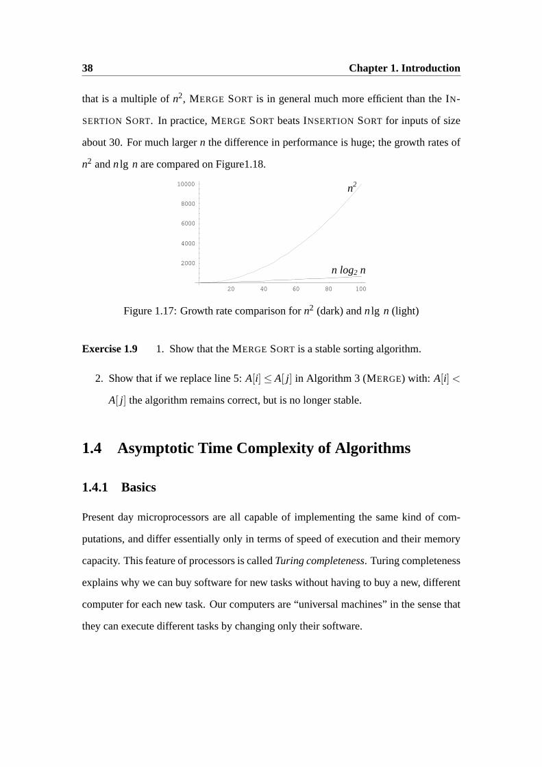
38 Chapter 1. Introduction
that is a multiple ofn2, MERGE SORT is in general much more efficient than theIN-
SERTION SORT. In practice,MERGE SORT beatsINSERTION SORT for inputs of size
about 30. For much largern the difference in performance is huge; the growth rates of
n2 andnlg n are compared on Figure1.18.
20 40 60 80 100
2000
4000
6000
8000
10000
n2
n log2 n
Figure 1.17: Growth rate comparison forn2 (dark) andnlg n (light)
Exercise 1.9 1. Show that theMERGESORT is a stable sorting algorithm.
2. Show that if we replace line 5:A[i]≤ A[ j] in Algorithm 3 (MERGE) with: A[i] <
A[ j] the algorithm remains correct, but is no longer stable.
1.4 Asymptotic Time Complexity of Algorithms
1.4.1 Basics
Present day microprocessors are all capable of implementing the same kind of com-
putations, and differ essentially only in terms of speed of execution and their memory
capacity. This feature of processors is calledTuring completeness. Turing completeness
explains why we can buy software for new tasks without having to buy a new, different
computer for each new task. Our computers are “universal machines” in the sense that
they can execute different tasks by changing only their software.
1.4. Asymptotic Time Complexity of Algorithms 39
Nearly all processors of the type that is commonly used in general purpose com-
puters are built according to the same architecture, usually called theVon Neumann
Architecture. They all consist of a CPU (Central Processing Unit) and a (potentially
infinite) collection of memory cells that can each be directly accessed, calledRandom
Access Memory(RAM). All such machines are equivalent to a theoretical model of
computation, called the Universal Turing Machine and thus are equally powerful com-
puting machines (save memory and speed constraints).
Two different (sequential) processorsA,B may have different “hard-wired” basic
operations, i.e., different sets of instructions implemented in the hardware by special
circuits. Since they can perform the same tasks, every instruction executable as a basic
instruction ofA, if not hard-wired inB, can be implemented as a sequence of steps of
instructions ofB. Since there are only finitely many basic instructions implemented in
the hardware ofA, there exists a natural numberM such that every basic instruction
of A can be implemented as a sequence of at mostM basic instructions ofB. Thus, a
programp containing only basic instructions available onA can replaced by a program
containing only instructions available onB, such thatp′ is at most as long asM times
the length ofp. Consequently, execution time of the same algorithm onA andB for the
same input can differ by at most a multiplicative constantM.
Since algorithms to be run on a processor of Von Neumann Architecture machines
are abstract entities independent of individual platforms on which they can be executed,
we need a method for measuring the execution time of an algorithm that is independent
for inessential features of the algorithm, such as which particular basic instructions are
used in specifying the algorithm. In light of the above discussion, we want to consider
two algorithms with execution times that, for sufficiently large inputs, differ by at most
a multiplicative constant as equally efficient. This leads us to the notion of asymptotic
40 Chapter 1. Introduction
growth rate of functions.
1.4.2 Asymptotic growth rate of functions
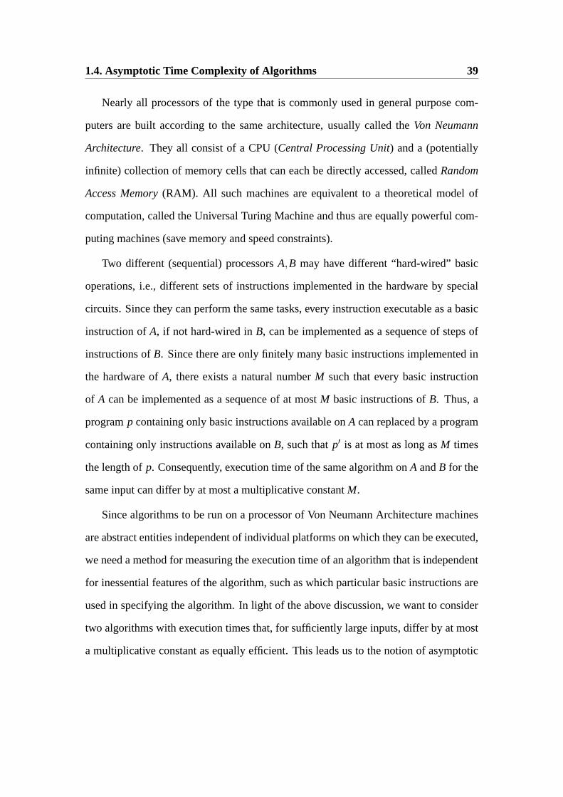
“Big Oh notation”: f (n) = O(g(n)) is abbreviation for the statement“There exists
positive constantsc andn0 such that0≤ f (n) ≤ cg(n) f oralln ≥ n0”. In this case we
say thatg(n) is an asymptotic upper bound forf (n).
Thus, f (n) = O(g(n)) means thatf (n) does not grow substantially faster thang(n)
because a multiple ofg(n) eventually dominatesf (n). Clearly, multiplying constants
of interest will be larger than1, thus “enlarging”g(n).
2g(x)
g(x)
f(x)
Figure 1.18:f (x) = O(g(x)); c = 2 andn0 = 18. Thus, f (x)≤ 2g(x) for n≥ 18
Example 1.8
1.4. Asymptotic Time Complexity of Algorithms 41
1. f (n) = n2 +10n does not grow substantially faster thang(n) = n2 in the sense of
the above definition becausef (n) = n2+10n≤ 2n2 = 2g(n) for all n≥ 10. Thus,
here we can takec = 2, n0 = 10, and son2 +10n = O(n2).
2. f (n) = 1000n2 does not grow substantially faster thang(n) = n2 becausef (n) =
1000n2 = 1000g(n) for all n≥ 0. Thus, forc= 1000andn0 = 0 we get1000n2 =
O(n2).
3. f (n) = n2 does grow substantially faster thang(n) = 1000n because there are
no constantsc,n0 such thatf (n) = n2 ≤ c1000n for all n≥ n0. This is because
n≥ 1000c impliesn2 > 1000cn. Consequently,1000n = O(n2).
Thus, a linear function can never be an asymptotic upper bound for a quadratic function.
“Omega notation”: f (n) = Ω(g(n)) is an abbreviation for the statement“There exists
positive constantsc andn0 such that0≤ cg(n) ≤ f (n) for all n≥ n0.” In this case we
say thatg(n) is an asymptotic lower bound forf (n).
Thus, f (n) = Ω(g(n)) essentially says thatf (n) grows at least as fast asg(n), be-
causef (n) eventually dominates a multiple of g(n). Clearly, multiplying constants of
interest will be smaller than1, thus ”reducing” g(n) by a constant factor.
Example 1.9
1. g(n) = 10n is an asymptotic lower bound forf (n) = n2 because whenn is suffi-
ciently large (n > 10) we haveg(n) = 10n < n2 = f (n). Thus, here we can take
c = 1 andn0 = 10.
42 Chapter 1. Introduction
2. g(n) = n2 is not an asymptotic lower bound forf (n) = 10n because there is no
constantc such that10n> cn2 for sufficiently largen. No matter how smallc> 0
is chosen,cn2 will eventually be larger than10n.
“Theta notation”: f (n) = Θ(g(n)) stands forf (n) = O(g(n)) and f (n) = Ω(g(n)). In
this case we say thatf andg have the same asymptotic growth rate, or that areasymp-
totically equivalent.
Thus, f (n) = Θ(g(n)) means thatg(n) is both an asymptotical upper bound and an
asymptotical lower bound forf (n). It is easy to see that in this case there exist positive
constantsc1,c2 andn0 such that0≤ c1 g(n)≤ f (n)≤ c2 g(n) for all n≥ n0.
Example 1.10
1. n2+5n+1= Θ(n2) because0≤ n2≤ n2+5n+1≤ 2n2 for all n≥ 6. In general,
for any polynomialp(x) of orderk we havep(x) = Θ(xk).
2. 2n+1 = Θ(2n) because0≥ 2n≥ 2n+1 = 2·2n for all n≥ 0.
1.4.3 Basic property of logarithms
1.9 The Logarithm function is very important for estimating the run time of algorithms.
For example, we have seen that theMERGE SORT algorithm runs in timeO(nlg (n)).
1.4. Asymptotic Time Complexity of Algorithms 43
We now review briefly the main properties of the logarithm function.
logc(ab) = logca+ logcb (1.3)
logc(a/b) = logca− logcb (1.4)
log(ab) = b loga (1.5)
alogab = b (1.6)
logax = logbx logab = logbx/ logba (1.7)
Proof: Properties 1.3 - 1.5 follow directly from the definition of thelog function, i.e.,
from the fact thatlogcx = y just in casecy = x, and the corresponding basic proper-
ties of exponentiation:cx+y = cxcy; cx−y = cx/cy; (cx)y = cxy. Property 1.7 is a bit
trickier: let logbx = w; thus, bw = x. Using 1.6 and substituting inbw = x we get
(alogab)w = x, i.e.,awlogab = x. Take nowloga of both sides to getwlogab= logax, i.e.,
logbxlogab = logax. 2
Note that 1.7 implies that for every two numbersa,b> 1we havelogan= Θ(logbn).
1.10 The growth rate of the factorial function. We now show thatlg n! = Θ(n lg n).
Using Stirling’s formulan! =√
2πn(
ne
)(1+ Θ(1/n)) and takinglg of both sides we
get:
lg (n!) = lg√
2πn+n lg n−n lg e+ lg (1+Θ(1/n))
However, it is easy to see that the expression on the right isΘ(n lg n).
44 Chapter 1. Introduction
Exercise 1.10Provelg (n!) = Θ(n lg n) using basic algebra only.
Hint: Note that forn > 0, n! ≤ nn and take logarithm of both sides; for the other
direction show thatnn < (n!)2 by pairing suitably factors of(n!)2 and then using the
fact thatx(n+1− x) < n for all 1≤ x≤ n. This inequality can be proved using basic
algebra of quadratic polynomials.
Exercise 1.11Determine iff (n) = O(g(n)), f (n) = Ω(g(n)) or f (n) = Θ(g(n)) for the
following pairs:
f (n) g(n)
n (n−2 lg n)(n+cos n)
(lg n)2 lg (nlg n)+2 lg n
n1+sin(π n/2))/2 √n (a plot might help)
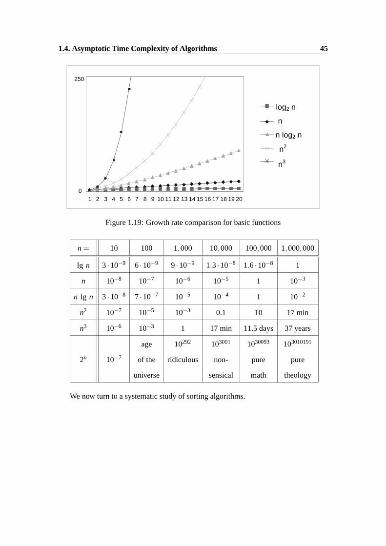
How important is the run time of an algorithm? Is it just the matter of “elegance”?
The graph on the Figure 1.19 might help explain the significance of algorithm effi-
ciency. To comprehend the growth rate of these functions even better, assume we have
algorithms with time complexities shown in the table, that are executed on a 1 GHz
machine executing one instruction each clock cycle. In the table one can find how long
it would take to complete these programs; time is in seconds unless stated otherwise.
For many real-time applications, for example algorithms used in digital telecom-
munications, algorithms that run in quadratic time are unacceptably slow. For standard
applications cubic run time is unacceptably slow, unless inputs are of relatively small
size. ”Brute force” algorithms often tend to run in exponential time, and as you can
see, for inputs of size only 100 it would take the entire age of the universe! Thus, poor
efficiency of an algorithm can often render it entirely useless.
1.4. Asymptotic Time Complexity of Algorithms 45
log2 n
n
n log2 n
n2
n3
0
250
1 2 3 4 5 6 7 8 9 10 11 12 13 14 15 16 17 18 19 20
Figure 1.19: Growth rate comparison for basic functions
n = 10 100 1,000 10,000 100,000 1,000,000
lg n 3·10−9 6·10−9 9·10−9 1.3·10−8 1.6·10−8 1
n 10−8 10−7 10−6 10−5 1 10−3
n lg n 3·10−8 7·10−7 10−5 10−4 1 10−2
n2 10−7 10−5 10−3 0.1 10 17 min
n3 10−6 10−3 1 17 min 11.5 days 37 years
age 10292 103001 1030093 103010191
2n 10−7 of the ridiculous non- pure pure
universe sensical math theology
We now turn to a systematic study of sorting algorithms.

Chapter 2
Sorting Algorithms
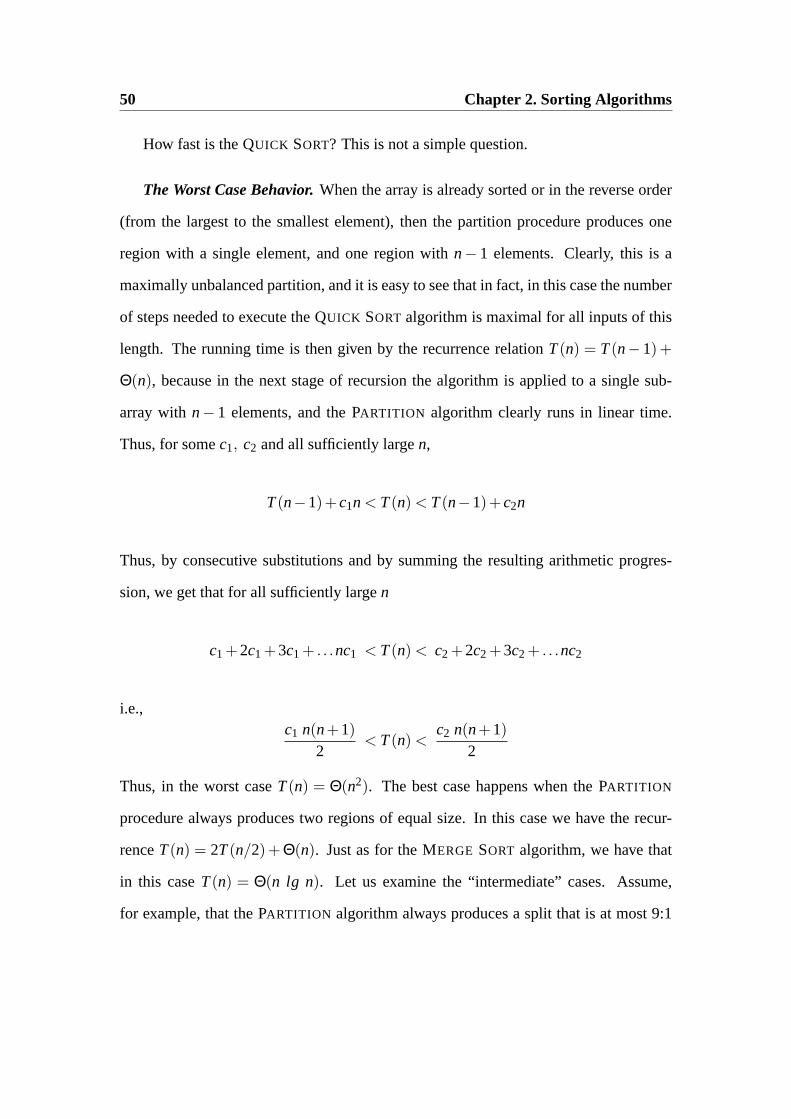
Sorting is one of the most frequently encountered data processing tasks. There are
many sorting algorithms, and one could wonder why there are so many algorithms for
the same task. We will see that for different probability distributions of inputs, different
algorithms for the same task can have vastly different performance. For example, we
have seen thatINSERTION SORT is extremely fast if inputs are nearly sorted; on such
inputs it runs in linear time. However, if all permutations of inputs are equally likely,
then INSERTION SORT is extremely slow; for such inputs it runs in quadratic time.
Merge Sort , on the other hand, runs in timeΘ(n lgn) for all inputs, but the constants
involved in this asymptotic bound are not very small. For that reason, theMERGE
SORT algorithm is rather slow for smaller size inputs (less than about 30-40 elements).
We will study another sorting algorithm, theQUICK SORT, that has very low average
sorting time for random inputs, but if inputs are frequently nearly sorted, thenQUICK
SORT is very slow: it runs in quadratic time.Thus, the choice of a sorting algorithms
depends on the expected input.
Besides being important on their own right as massively used tools, sorting algo-
47
48 Chapter 2. Sorting Algorithms
rithms will be also used to illustrate:
1. how to chose the right algorithm for the task at hand;
2. general algorithm design techniques, like divide-and-conquer;
3. how to estimate time complexity of algorithms in general.
2.1 The Quick Sort
The Quick Sort is one of the most frequently used sorting algorithms. Assume that we
want to sort the part of an arrayA that is between indicesp andr, i.e., to sortA[p. . . r].
We employ “divide-and-conquer” strategy, as follows:
Divide: The arrayA[p. . . r] is partitioned and rearranged into two nonempty sub-arrays
A[p. . .q] andA[q+1. . . r] such that every element ofA[p. . .q] is smaller or equal than
A[p], chosen to bethe pivoting element, and every element ofA[q+1. . . r] is larger or
equal thanA[p]. Thus, each element ofA[p. . .q] is smaller or equal than every element
of A[q+1. . . r].
Conquer: The two sub-arraysA[p. . .q] andA[q+1. . . r] are sorted by recursive calls
to QUICK SORT.
Combine:Since both sub-arrays are now sorted in place, no work is needed to combine
them; the entire arrayA[p. . . r] is already sorted.
We first describe thePARTITION procedure which rearranges and splits the array.
2.1. The Quick Sort 49
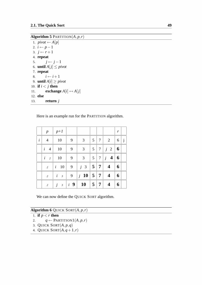
Algorithm 5 PARTITION(A, p, r)1. pivot← A[p]2. i ← p−13. j ← r +14. repeat5. j ← j−16. until A[ j]≤ pivot7. repeat8. i ← i +19. until A[i]≥ pivot
10. if i < j then11. exchangeA[i]↔ A[ j]12. else13. return j
Here is an example run for thePARTITION algorithm.
p p+1 r
i 4 10 9 3 5 7 2 6 j
i 4 10 9 3 5 7 j 2 6
i 2 10 9 3 5 7 j 4 6
2 i 10 9 j 3 5 7 4 6
2 i 3 9 j 10 5 7 4 6
2 j 3 i 9 10 5 7 4 6
We can now define theQUICK SORT algorithm.
Algorithm 6 QUICK SORT(A, p, r)1. if p < r then2. q← PARTITION1(A, p, r)3. QUICK SORT(A, p,q)4. QUICK SORT(A,q+1, r)
50 Chapter 2. Sorting Algorithms
How fast is theQUICK SORT? This is not a simple question.
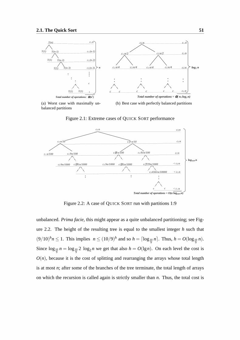
The Worst Case Behavior.When the array is already sorted or in the reverse order
(from the largest to the smallest element), then the partition procedure produces one
region with a single element, and one region withn− 1 elements. Clearly, this is a
maximally unbalanced partition, and it is easy to see that in fact, in this case the number
of steps needed to execute theQUICK SORT algorithm is maximal for all inputs of this
length. The running time is then given by the recurrence relationT(n) = T(n−1)+
Θ(n), because in the next stage of recursion the algorithm is applied to a single sub-
array withn− 1 elements, and thePARTITION algorithm clearly runs in linear time.
Thus, for somec1, c2 and all sufficiently largen,
T(n−1)+c1n < T(n) < T(n−1)+c2n
Thus, by consecutive substitutions and by summing the resulting arithmetic progres-
sion, we get that for all sufficiently largen
c1 +2c1 +3c1 + . . .nc1 < T(n) < c2 +2c2 +3c2 + . . .nc2
i.e.,c1 n(n+1)
2< T(n) <
c2 n(n+1)2
Thus, in the worst caseT(n) = Θ(n2). The best case happens when thePARTITION
procedure always produces two regions of equal size. In this case we have the recur-
renceT(n) = 2T(n/2)+ Θ(n). Just as for theMERGE SORT algorithm, we have that
in this caseT(n) = Θ(n lg n). Let us examine the “intermediate” cases. Assume,
for example, that thePARTITION algorithm always produces a split that is at most 9:1
2.1. The Quick Sort 51
n
T(n)
T(1)
c⋅⋅⋅⋅ n
c⋅⋅⋅⋅ (n-1)
Total number of operations: ΘΘΘΘ(n2)
: :
T(1)
T(1)
T(n-1)
T(n-2)
T(n-3)
T(1) T(1)
:
c⋅⋅⋅⋅ (n-2)
c⋅⋅⋅⋅ (n-3)
c
: :
c
(a) Worst case with maximally un-balanced partitions
log2 n
c⋅⋅⋅⋅ n
c⋅⋅⋅⋅ n/2 c⋅⋅⋅⋅ n/2
c⋅⋅⋅⋅ n/4 c⋅⋅⋅⋅ n/4 c⋅⋅⋅⋅ n/4
c⋅⋅⋅⋅ n
c⋅⋅⋅⋅ n
c⋅⋅⋅⋅ n
c⋅⋅⋅⋅ n
Total number of operations = ΘΘΘΘ( n⋅⋅⋅⋅ log2 n)
c c
: : : :
c c
: :
c c
: :
c⋅⋅⋅⋅ n/4
(b) Best case with perfectly balanced partitions
Figure 2.1: Extreme cases ofQUICK SORT performance
log10/9 n
c⋅⋅⋅⋅ n
c⋅⋅⋅⋅9 n/10
c⋅⋅⋅⋅ 81n/100
c⋅⋅⋅⋅ n
c⋅⋅⋅⋅ n
c⋅⋅⋅⋅ n
Total number of operations = O(n log10/9 n)
c
: :
c⋅⋅⋅⋅ n/100
c⋅⋅⋅⋅ n/10
c⋅⋅⋅⋅ 9n/100
c⋅⋅⋅⋅ 9n/1000 c⋅⋅⋅⋅ 81n/1000
:
c⋅⋅⋅⋅9 n/100
c⋅⋅⋅⋅ 9n/1000 c⋅⋅⋅⋅ 81n/1000
:
c⋅⋅⋅⋅ 729n/1000
c⋅⋅⋅⋅ 6561n/10000
c
< c⋅⋅⋅⋅ n
< c⋅⋅⋅⋅ n
< c⋅⋅⋅⋅ n
Figure 2.2: A case ofQUICK SORT run with partitions 1:9
unbalanced.Prima facie,this might appear as a quite unbalanced partitioning; see Fig-
ure 2.2. The height of the resulting tree is equal to the smallest integerh such that
(9/10)hn≤ 1. This implies n≤ (10/9)h and soh = dlog109
ne. Thus,h = O(log109
n).
Sincelog109
n = log109
2 log2n we get that alsoh = O(lgn). On each level the cost is
O(n), because it is the cost of splitting and rearranging the arrays whose total length
is at mostn; after some of the branches of the tree terminate, the total length of arrays
on which the recursion is called again is strictly smaller thann. Thus, the total cost is
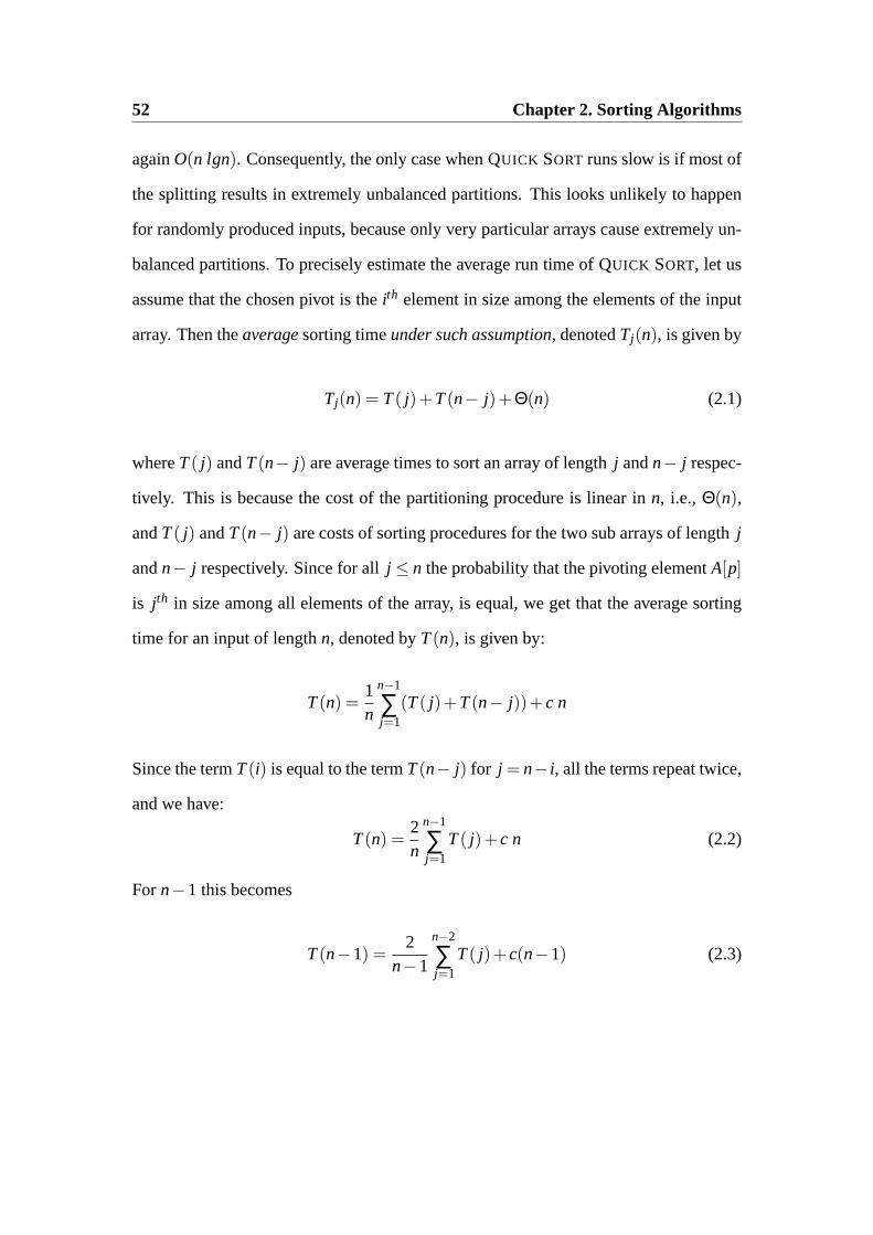
52 Chapter 2. Sorting Algorithms
againO(n lgn). Consequently, the only case whenQUICK SORT runs slow is if most of
the splitting results in extremely unbalanced partitions. This looks unlikely to happen
for randomly produced inputs, because only very particular arrays cause extremely un-
balanced partitions. To precisely estimate the average run time ofQUICK SORT, let us
assume that the chosen pivot is theith element in size among the elements of the input
array. Then theaveragesorting timeunder such assumption, denotedTj(n), is given by
Tj(n) = T( j)+T(n− j)+Θ(n) (2.1)
whereT( j) andT(n− j) are average times to sort an array of lengthj andn− j respec-
tively. This is because the cost of the partitioning procedure is linear inn, i.e., Θ(n),
andT( j) andT(n− j) are costs of sorting procedures for the two sub arrays of lengthj
andn− j respectively. Since for allj ≤ n the probability that the pivoting elementA[p]
is jth in size among all elements of the array, is equal, we get that the average sorting
time for an input of lengthn, denoted byT(n), is given by:
T(n) =1n
n−1
∑j=1
(T( j)+T(n− j))+c n
Since the termT(i) is equal to the termT(n− j) for j = n− i, all the terms repeat twice,
and we have:
T(n) =2n
n−1
∑j=1
T( j)+c n (2.2)
Forn−1 this becomes
T(n−1) =2
n−1
n−2
∑j=1
T( j)+c(n−1) (2.3)
2.1. The Quick Sort 53
Multiplying the first equation byn and the second byn−1 and by subtracting, we get
nT(n)− (n−1)T(n−1) = 2T(n−1)+c(n2− (n−1)2) (2.4)
because all terms of the second sum cancel the corresponding term of the first sum,
leaving only2T(n−1), that is not present in the second sum. Thus,
nT(n)− (n+1)T(n−1) = c(2n+1) (2.5)
which, by dividing both sides byn(n+1), becomes
T(n)n+1
− T(n−1)n
=c(2n+1)n(n+1)
<2cn
(2.6)
i.e.,T(n)n+1
<T(n−1)
n+
2cn
(2.7)
By applying the same fact onT(n−1) we get
T(n−1)n
<T(n−2)
n−1+
2cn−1
(2.8)
by combining 2.7 and 2.8 we get
T(n)n
<T(n−2)
n−1+
2cn
+2c
n−1(2.9)
Applying 2.7 toT(n−2) and continuing in the above manner, we get
T(n)n
< 2cn
∑i=1
1i
(2.10)
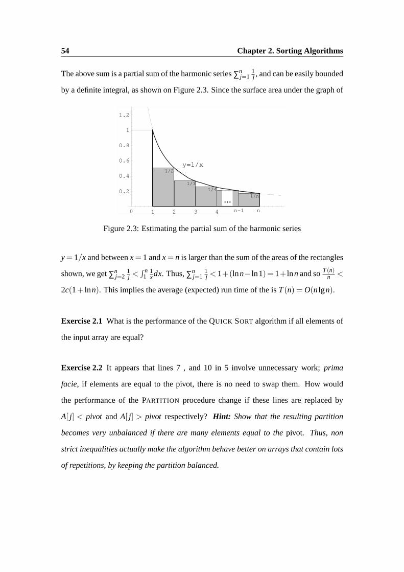
54 Chapter 2. Sorting Algorithms
The above sum is a partial sum of the harmonic series∑nj=1
1j , and can be easily bounded
by a definite integral, as shown on Figure 2.3. Since the surface area under the graph of
1 2 3 4 5 6 7
0.2
0.4
0.6
0.8
1
1.2
y=1/x
1/4
1/2
1/3
1/n ... n-1 n 0
Figure 2.3: Estimating the partial sum of the harmonic series
y= 1/x and betweenx= 1 andx= n is larger than the sum of the areas of the rectangles
shown, we get∑nj=2
1j <
∫ n1
1xdx. Thus,∑n
j=11j < 1+(lnn− ln1) = 1+ lnn and soT(n)
n <
2c(1+ lnn). This implies the average (expected) run time of the isT(n) = O(nlgn).
Exercise 2.1What is the performance of theQUICK SORT algorithm if all elements of
the input array are equal?
Exercise 2.2 It appears that lines 7 , and 10 in 5 involve unnecessary work;prima
facie, if elements are equal to the pivot, there is no need to swap them. How would
the performance of thePARTITION procedure change if these lines are replaced by
A[ j] < pivot and A[ j] > pivot respectively?Hint: Show that the resulting partition
becomes very unbalanced if there are many elements equal to thepivot. Thus, non
strict inequalities actually make the algorithm behave better on arrays that contain lots
of repetitions, by keeping the partition balanced.
2.1. The Quick Sort 55
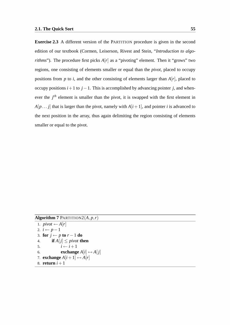
Exercise 2.3A different version of thePARTITION procedure is given in the second
edition of our textbook (Cormen, Leiserson, Rivest and Stein, “Introduction to algo-
rithms”). The procedure first picksA[r] as a “pivoting” element. Then it “grows” two
regions, one consisting of elements smaller or equal than thepivot, placed to occupy
positions fromp to i, and the other consisting of elements larger thanA[r], placed to
occupy positionsi +1 to j−1. This is accomplished by advancing pointerj, and when-
ever the jth element is smaller than the pivot, it is swapped with the first element in
A[p. . . j] that is larger than the pivot, namely withA[i +1], and pointeri is advanced to
the next position in the array, thus again delimiting the region consisting of elements
smaller or equal to the pivot.
Algorithm 7 PARTITION2(A, p, r)1. pivot← A[r]2. i ← p−13. for j ← p to r−1 do4. if A[ j]≤ pivot then5. i ← i +16. exchangeA[i]↔ A[ j]7. exchangeA[i +1]↔ A[r]8. return i +1
56 Chapter 2. Sorting Algorithms
p p+4 r
i j 4 10 9 3 5 7 2 6
i 4 j 10 9 3 5 7 2 6
i 4 10 j 9 3 5 7 2 6
i 4 10 9 j 3 5 7 2 6
4 i 3 9 10 j 5 7 2 6
4 3 i 5 10 9 j 7 2 6
4 3 i 5 10 9 7 j 2 6
4 3 5 i 2 9 7 10 6
4 3 5 i 2 6 7 10 9
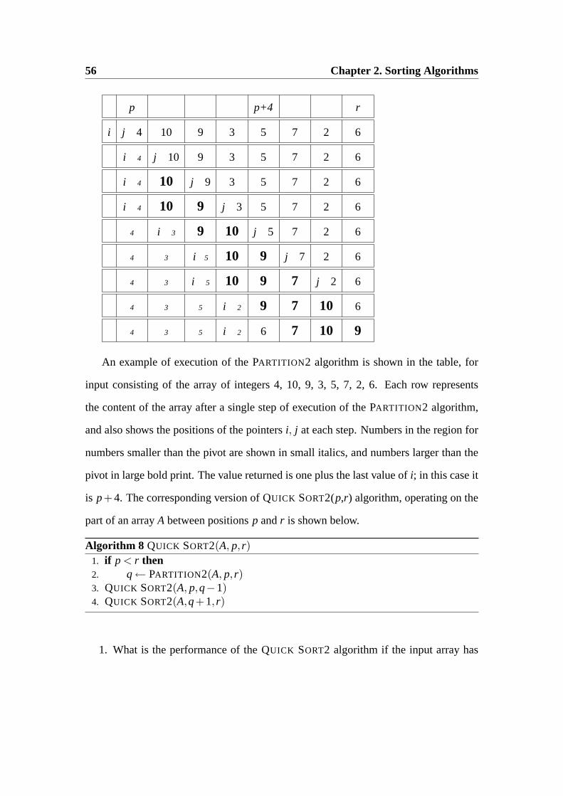
An example of execution of thePARTITION2 algorithm is shown in the table, for
input consisting of the array of integers 4, 10, 9, 3, 5, 7, 2, 6. Each row represents
the content of the array after a single step of execution of thePARTITION2 algorithm,
and also shows the positions of the pointersi, j at each step. Numbers in the region for
numbers smaller than the pivot are shown in small italics, and numbers larger than the
pivot in large bold print. The value returned is one plus the last value ofi; in this case it
is p+4. The corresponding version ofQUICK SORT2(p,r) algorithm, operating on the
part of an arrayA between positionsp andr is shown below.
Algorithm 8 QUICK SORT2(A, p, r)1. if p < r then2. q← PARTITION2(A, p, r)3. QUICK SORT2(A, p,q−1)4. QUICK SORT2(A,q+1, r)
1. What is the performance of theQUICK SORT2 algorithm if the input array has
2.1. The Quick Sort 57
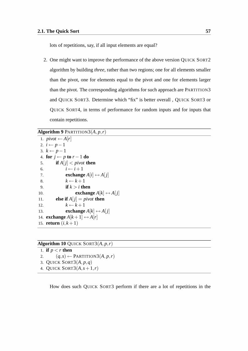
lots of repetitions, say, if all input elements are equal?
2. One might want to improve the performance of the above versionQUICK SORT2
algorithm by buildingthree, rather than two regions; one for all elements smaller
than the pivot, one for elements equal to the pivot and one for elements larger
than the pivot. The corresponding algorithms for such approach arePARTITION3
andQUICK SORT3. Determine which “fix” is better overall ,QUICK SORT3 or
QUICK SORT4, in terms of performance for random inputs and for inputs that
contain repetitions.
Algorithm 9 PARTITION3(A, p, r)1. pivot← A[r]2. i ← p−13. k← p−14. for j ← p to r−1 do5. if A[ j] < pivot then6. i ← i +17. exchangeA[i]↔ A[ j]8. k← k+19. if k > i then
10. exchangeA[k]↔ A[ j]11. else ifA[ j] = pivot then12. k← k+113. exchangeA[k]↔ A[ j]14. exchangeA[k+1]↔ A[r]15. return (i,k+1)
Algorithm 10 QUICK SORT3(A, p, r)1. if p < r then2. (q,s)← PARTITION3(A, p, r)3. QUICK SORT3(A, p,q)4. QUICK SORT3(A,s+1, r)
How does suchQUICK SORT3 perform if there are a lot of repetitions in the
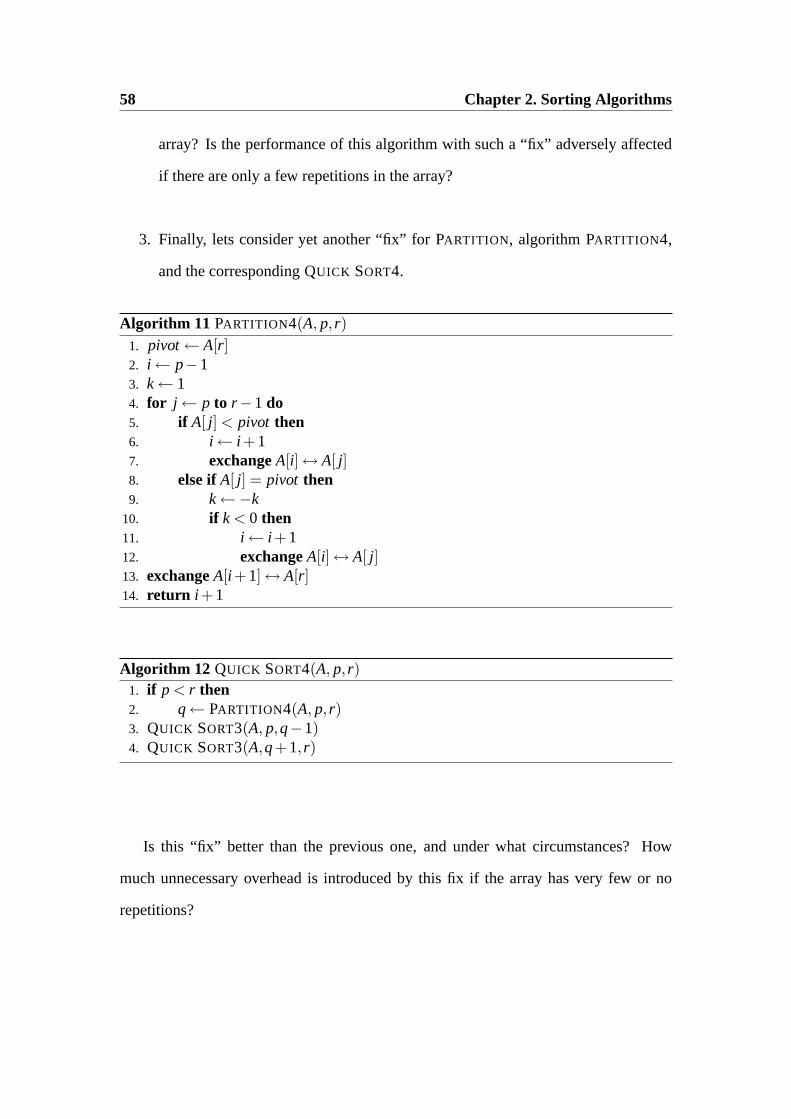
58 Chapter 2. Sorting Algorithms
array? Is the performance of this algorithm with such a “fix” adversely affected
if there are only a few repetitions in the array?
3. Finally, lets consider yet another “fix” forPARTITION, algorithmPARTITION4,
and the correspondingQUICK SORT4.
Algorithm 11 PARTITION4(A, p, r)1. pivot← A[r]2. i ← p−13. k← 14. for j ← p to r−1 do5. if A[ j] < pivot then6. i ← i +17. exchangeA[i]↔ A[ j]8. else ifA[ j] = pivot then9. k←−k
10. if k < 0 then11. i ← i +112. exchangeA[i]↔ A[ j]13. exchangeA[i +1]↔ A[r]14. return i +1
Algorithm 12 QUICK SORT4(A, p, r)1. if p < r then2. q← PARTITION4(A, p, r)3. QUICK SORT3(A, p,q−1)4. QUICK SORT3(A,q+1, r)
Is this “fix” better than the previous one, and under what circumstances? How
much unnecessary overhead is introduced by this fix if the array has very few or no
repetitions?
2.2. Randomization 59
2.2 Randomization
In practice, the Quick Sort is on average about twice as fast as the Merge Sort. However,
despite its low average run time, on particular inputs the Quick Sort can be extremely
slow: it might run in quadratic time. For example, if you use the Quick Sort to sort
checks in a bank, the performance of Quick Sort will be extremely poor, because checks
appear in nearly sorted order, and for such sequences the Quick Sort has quadratic run
time. However, it is easy to fix this problem of the Quick Sort algorithm. We can insure
that the performance of the Quick Sort algorithm on a large set of inputs is essentially
independent on the probability distribution of different permutations of input strings
by usingrandomization. Randomizationcannot guarantee good performance on any
particular input, but it brings theaveragerun time for this set of inputs closer to the
expected valueof the run time of the Quick Sort algorithm for random inputs, i.e.,
for inputs in which all permutations are equally likely. Thus, we can expect efficient
performance of the randomized Quick Sort algorithm on large sets of inputs.
Randomization is accomplished by picking the pivot from the input array randomly,
by first swapping the pivoting element with a randomly chosen element. Thus, for
example, Algorithm 5 is transformed in this way into Algorithm 13;RANDOM(p, r) is
a random number generator producing integers betweenp andr with (approximately)
equal probability.
Clearly, our analysis of the expected time of theQUICK SORT algorithm equally
applies to the expected time of theRANDOMIZED QUICK SORT algorithm. Note that
randomization doesnot reduce the expected run time, but only insures that no particular
permutation of input elicits slow performance of the algorithm.
Note that calling a random number generator at each call of thePARTITION algo-
60 Chapter 2. Sorting Algorithms
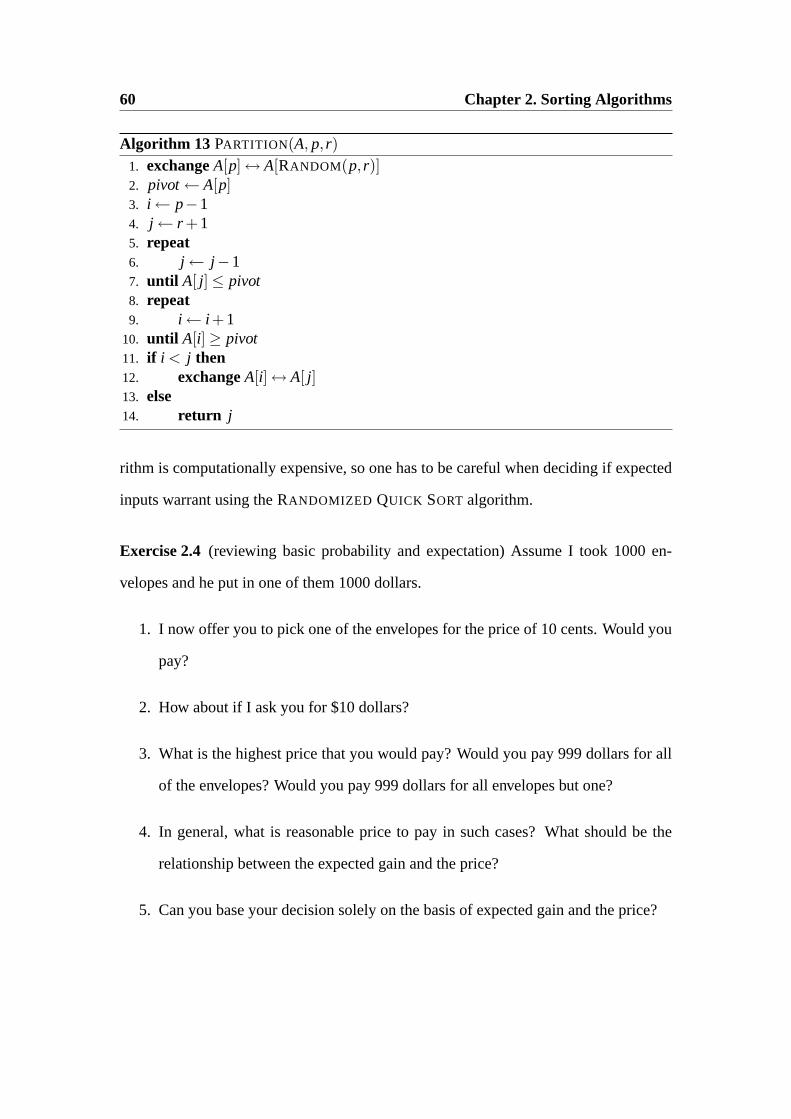
Algorithm 13 PARTITION(A, p, r)1. exchangeA[p]↔ A[RANDOM(p, r)]2. pivot← A[p]3. i ← p−14. j ← r +15. repeat6. j ← j−17. until A[ j]≤ pivot8. repeat9. i ← i +1
10. until A[i]≥ pivot11. if i < j then12. exchangeA[i]↔ A[ j]13. else14. return j
rithm is computationally expensive, so one has to be careful when deciding if expected
inputs warrant using theRANDOMIZED QUICK SORT algorithm.
Exercise 2.4 (reviewing basic probability and expectation) Assume I took 1000 en-
velopes and he put in one of them 1000 dollars.
1. I now offer you to pick one of the envelopes for the price of 10 cents. Would you
pay?
2. How about if I ask you for $10 dollars?
3. What is the highest price that you would pay? Would you pay 999 dollars for all
of the envelopes? Would you pay 999 dollars for all envelopes but one?
4. In general, what is reasonable price to pay in such cases? What should be the
relationship between the expected gain and the price?
5. Can you base your decision solely on the basis of expected gain and the price?
2.2. Randomization 61
Other methods for improving the performance of the Quick Sort involve ensuring
that we pick a good pivot (i.e., as close to the median of elements in the array, thus
ensuring a balanced ensuing partition. They include taking a median of three elements,
picked one from both ends of the array and one from the center. Also, when the size of
the input array becomes small, recursive divide and conquer becomes inefficient: small
size arrays are best sorted by the Insertion Sort. Thus, one improvement of the Quick
Sort involves stopping the recursive partitioning when the size of the array drops below
certain threshold, usually about 20 or so. Small size sub-arrays are left unsorted, until
the Quick Sort terminates, and then the resulting “nearly sorted” array is sorted in linear
time using Insertion Sort.
Since the efficiency of the Quick Sort comes from the simplicity of the inner loop,
as with randomization, every “improvement” must be carefully weighted against added
computational complexity. Lots of useful details on this topic can be found in Sedgewick’s
classical bookAlgorithms(editions are available with implementations for several lan-
guages, includingC, C++ andJava).