EUROPEAN ORGANIZATION FOR NUCLEAR RESEARCH (CERN)

CERN-PH-EP-2015-153LHCb-PAPER-2015-029

July 13, 2015

Observation of J/ψp resonancesconsistent with pentaquark states in

Λ0b → J/ψK−p decays

The LHCb collaboration1

Abstract

Observations of exotic structures in the J/ψp channel, which we refer to ascharmonium-pentaquark states, in Λ0

b → J/ψK−p decays are presented. The datasample corresponds to an integrated luminosity of 3 fb−1 acquired with the LHCbdetector from 7 and 8 TeV pp collisions. An amplitude analysis of the three-bodyfinal-state reproduces the two-body mass and angular distributions. To obtain asatisfactory fit of the structures seen in the J/ψp mass spectrum, it is necessaryto include two Breit-Wigner amplitudes that each describe a resonant state. Thesignificance of each of these resonances is more than 9 standard deviations. One hasa mass of 4380± 8± 29 MeV and a width of 205± 18± 86 MeV, while the second isnarrower, with a mass of 4449.8± 1.7± 2.5 MeV and a width of 39± 5± 19 MeV.The preferred JP assignments are of opposite parity, with one state having spin 3/2and the other 5/2.

Submitted to Phys. Rev. Lett.

c© CERN on behalf of the LHCb collaboration, license CC-BY-4.0.

1Authors are listed at the end of this Letter.

arX

iv:1

507.

0341

4v2

[he

p-ex

] 2

5 Ju

l 201

5

Introduction and summary

The prospect of hadrons with more than the minimal quark content (qq or qqq) wasproposed by Gell-Mann in 1964 [1] and Zweig [2], followed by a quantitative model for twoquarks plus two antiquarks developed by Jaffe in 1976 [3]. The idea was expanded upon [4]to include baryons composed of four quarks plus one antiquark; the name pentaquark wascoined by Lipkin [5]. Past claimed observations of pentaquark states have been shown tobe spurious [6], although there is at least one viable tetraquark candidate, the Z(4430)+

observed in B0 → ψ′K−π+ decays [7–9], implying that the existence of pentaquark baryonstates would not be surprising. States that decay into charmonium may have particularlydistinctive signatures [10].

Large yields of Λ0b → J/ψK−p decays are available at LHCb and have been used for

the precise measurement of the Λ0b lifetime [11]. (In this Letter mention of a particular

mode implies use of its charge conjugate as well.) This decay can proceed by the diagramshown in Fig. 1(a), and is expected to be dominated by Λ∗ → K−p resonances, as areevident in our data shown in Fig. 2(a). It could also have exotic contributions, as indicatedby the diagram in Fig. 1(b), that could result in resonant structures in the J/ψp massspectrum shown in Fig. 2(b).

Figure 1: Feynman diagrams for (a) Λ0b → J/ψΛ∗ and (b) Λ0

b → P+c K

− decay.

[GeV]pKm1.4 1.6 1.8 2.0 2.2 2.4

Eve

nts/

(20

MeV

)

500

1000

1500

2000

2500

3000

LHCb(a)

data

phase space

[GeV]pψ/Jm4.0 4.2 4.4 4.6 4.8 5.0

Eve

nts/

(15

MeV

)

200

400

600

800 LHCb(b)

Figure 2: Invariant mass of (a) K−p and (b) J/ψp combinations from Λ0b → J/ψK−p decays.

The solid (red) curve is the expectation from phase space. The background has been subtracted.

1

In practice resonances decaying strongly into J/ψp must have a minimal quark contentof ccuud, and thus are charmonium-pentaquarks; we label such states P+

c , irrespective ofthe internal binding mechanism. In order to ascertain if the structures seen in Fig. 2(b)are resonant in nature and not due to reflections generated by the Λ∗ states, it is necessaryto perform a full amplitude analysis, allowing for interference effects between both decaysequences.

The fit uses five decay angles and the K−p invariant mass mKp as independent variables.First we tried to fit the data with an amplitude model that contains 14 Λ∗ states listed bythe Particle Data Group [12]. As this did not give a satisfactory description of the data,we added one P+

c state, and when that was not sufficient we included a second state. Thetwo P+

c states are found to have masses of 4380± 8± 29 MeV and 4449.8± 1.7± 2.5 MeV,with corresponding widths of 205± 18± 86 MeV and 39± 5± 19 MeV. (Natural units areused throughout this Letter. Whenever two uncertainties are quoted the first is statisticaland the second systematic.) The fractions of the total sample due to the lower mass andhigher mass states are (8.4± 0.7± 4.2)% and (4.1± 0.5± 1.1)%, respectively. The best fitsolution has spin-parity JP values of (3/2−, 5/2+). Acceptable solutions are also foundfor additional cases with opposite parity, either (3/2+, 5/2−) or (5/2+, 3/2−). The bestfit projections are shown in Fig. 3. Both mKp and the peaking structure in mJ/ψp arereproduced by the fit. The significances of the lower mass and higher mass states are 9and 12 standard deviations, respectively.

[GeV]pKm1.4 1.6 1.8 2 2.2 2.4 2.6

Eve

nts/

(15

MeV

)

0

200

400

600

800

1000

1200

1400

1600

1800

2000

2200

LHCb(a)

datatotal fitbackground

(4450)cP(4380)cP(1405)Λ(1520)Λ(1600)Λ(1670)Λ(1690)Λ(1800)Λ(1810)Λ(1820)Λ(1830)Λ(1890)Λ(2100)Λ(2110)Λ

[GeV]pψ/Jm4 4.2 4.4 4.6 4.8 5

Eve

nts/

(15

MeV

)

0

100

200

300

400

500

600

700

800

LHCb(b)

Figure 3: Fit projections for (a) mKp and (b) mJ/ψp for the reduced Λ∗ model with two P+c states

(see Table 1). The data are shown as solid (black) squares, while the solid (red) points show theresults of the fit. The solid (red) histogram shows the background distribution. The (blue) opensquares with the shaded histogram represent the Pc(4450)+ state, and the shaded histogramtopped with (purple) filled squares represents the Pc(4380)+ state. Each Λ∗ component is alsoshown. The error bars on the points showing the fit results are due to simulation statistics.

2

Analysis and results

We use data corresponding to 1 fb−1 of integrated luminosity acquired by the LHCbexperiment in pp collisions at 7 TeV center-of-mass energy, and 2 fb−1 at 8 TeV. TheLHCb detector [13] is a single-arm forward spectrometer covering the pseudorapidity range2 < η < 5. The detector includes a high-precision tracking system consisting of a silicon-strip vertex detector surrounding the pp interaction region [14], a large-area silicon-stripdetector located upstream of a dipole magnet with a bending power of about 4 Tm, andthree stations of silicon-strip detectors and straw drift tubes [15] placed downstream ofthe magnet. Different types of charged hadrons are distinguished using information fromtwo ring-imaging Cherenkov detectors [16]. Muons are identified by a system composed ofalternating layers of iron and multiwire proportional chambers [17].

Events are triggered by a J/ψ → µ+µ− decay, requiring two identified muons withopposite charge, each with transverse momentum, pT, greater than 500 MeV. The dimuonsystem is required to form a vertex with a fit χ2 < 16, to be significantly displaced fromthe nearest pp interaction vertex, and to have an invariant mass within 120 MeV of theJ/ψ mass [12]. After applying these requirements, there is a large J/ψ signal over a smallbackground [18]. Only candidates with dimuon invariant mass between −48 MeV and+43 MeV relative to the observed J/ψ mass peak are selected, the asymmetry accountingfor final-state electromagnetic radiation.

Analysis preselection requirements are imposed prior to using a gradient BoostedDecision Tree, BDTG [19], that separates the Λ0

b signal from backgrounds. Each trackis required to be of good quality and multiple reconstructions of the same track areremoved. Requirements on the individual particles include pT > 550 MeV for muons, andpT > 250 MeV for hadrons. Each hadron must have an impact parameter χ2 with respectto the primary pp interaction vertex larger than 9, and must be positively identified in theparticle identification system. The K−p system must form a vertex with χ2 < 16, as mustthe two muons from the J/ψ decay. Requirements on the Λ0

b candidate include a vertexχ2 < 50 for 5 degrees of freedom, and a flight distance of greater than 1.5 mm. The vectorfrom the primary vertex to the Λ0

b vertex must align with the Λ0b momentum so that the

cosine of the angle between them is larger than 0.999. Candidate µ+µ− combinations areconstrained to the J/ψ mass for subsequent use in event selection.

The BDTG technique involves a “training” procedure using sideband data backgroundand simulated signal samples. (The variables used are listed in the supplementary material.)We use 2× 106 Λ0

b → J/ψK−p events with J/ψ → µ+µ− that are generated uniformly inphase space in the LHCb acceptance, using Pythia [20] with a special LHCb parametertune [21], and the LHCb detector simulation based on Geant4 [22], described in Ref. [23].The product of the reconstruction and trigger efficiencies within the LHCb geometricacceptance is about 10%. In addition, specific backgrounds from B0

s and B0 decaysare vetoed. This is accomplished by removing combinations that when interpreted asJ/ψK+K− fall within ±30 MeV of the B0

s mass or when interpreted as J/ψK−π+ fallwithin ±30 MeV of the B0 mass. This requirement effectively eliminates backgroundfrom these sources and causes only smooth changes in the detection efficiencies across the

3

[MeV]5500 5600 5700

Eve

nts

/ ( 4

MeV

)

0

1000

2000

3000

4000

5000

6000

7000LHCb

p ψ/Jm K

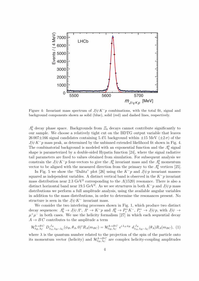
Figure 4: Invariant mass spectrum of J/ψK−p combinations, with the total fit, signal andbackground components shown as solid (blue), solid (red) and dashed lines, respectively.

Λ0b decay phase space. Backgrounds from Ξb decays cannot contribute significantly to

our sample. We choose a relatively tight cut on the BDTG output variable that leaves26 007±166 signal candidates containing 5.4% background within ±15 MeV (±2σ) of theJ/ψK−p mass peak, as determined by the unbinned extended likelihood fit shown in Fig. 4.The combinatorial background is modeled with an exponential function and the Λ0

b signalshape is parameterized by a double-sided Hypatia function [24], where the signal radiativetail parameters are fixed to values obtained from simulation. For subsequent analysis weconstrain the J/ψK−p four-vectors to give the Λ0

b invariant mass and the Λ0b momentum

vector to be aligned with the measured direction from the primary to the Λ0b vertices [25].

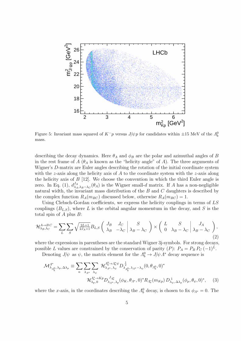
In Fig. 5 we show the “Dalitz” plot [26] using the K−p and J/ψp invariant masses-squared as independent variables. A distinct vertical band is observed in the K−p invariantmass distribution near 2.3 GeV2 corresponding to the Λ(1520) resonance. There is also adistinct horizontal band near 19.5 GeV2. As we see structures in both K−p and J/ψp massdistributions we perform a full amplitude analysis, using the available angular variablesin addition to the mass distributions, in order to determine the resonances present. Nostructure is seen in the J/ψK− invariant mass.

We consider the two interfering processes shown in Fig. 1, which produce two distinctdecay sequences: Λ0

b → J/ψΛ∗, Λ∗ → K−p and Λ0b → P+

c K−, P+

c → J/ψp, with J/ψ →µ+µ− in both cases. We use the helicity formalism [27] in which each sequential decayA→ B C contributes to the amplitude a term

HA→BCλB , λC

D JAλA, λB−λC (φB, θA, 0)∗RA(mBC) = HA→BC

λB , λCei λA φB d JA

λA, λB−λC (θA)RA(mBC), (1)

where λ is the quantum number related to the projection of the spin of the particle ontoits momentum vector (helicity) and HA→BC

λB , λCare complex helicity-coupling amplitudes

4

]2 [GeVKp2m

2 3 4 5 6

]2 [G

eVp

ψJ/2

m

16

18

20

22

24

26 LHCb

Figure 5: Invariant mass squared of K−p versus J/ψp for candidates within ±15 MeV of the Λ0b

mass.

describing the decay dynamics. Here θA and φB are the polar and azimuthal angles of Bin the rest frame of A (θA is known as the “helicity angle” of A). The three arguments ofWigner’s D-matrix are Euler angles describing the rotation of the initial coordinate systemwith the z-axis along the helicity axis of A to the coordinate system with the z-axis alongthe helicity axis of B [12]. We choose the convention in which the third Euler angle iszero. In Eq. (1), dJAλA,λB−λC (θA) is the Wigner small-d matrix. If A has a non-negligiblenatural width, the invariant mass distribution of the B and C daughters is described bythe complex function RA(mBC) discussed below, otherwise RA(mBC) = 1.

Using Clebsch-Gordan coefficients, we express the helicity couplings in terms of LScouplings (BL,S), where L is the orbital angular momentum in the decay, and S is thetotal spin of A plus B:

HA→BCλB ,λC

=∑L

∑S

√2L+1

2JA+1BL,S

(JB JC SλB −λC λB − λC

)×(L S JA0 λB − λC λB − λC

),

(2)where the expressions in parentheses are the standard Wigner 3j-symbols. For strong decays,possible L values are constrained by the conservation of parity (P ): PA = PB PC (−1)L.

Denoting J/ψ as ψ, the matrix element for the Λ0b → J/ψΛ∗ decay sequence is

MΛ∗

λΛ0b, λp,∆λµ ≡

∑n

∑λΛ∗

∑λψ

HΛ0b→Λ

∗nψ

λΛ∗ , λψD

12λΛ0b, λΛ∗−λψ(0, θΛ0

b, 0)∗

HΛ∗n→Kpλp, 0

DJΛ∗nλΛ∗ , λp

(φK , θΛ∗ , 0)∗RΛ∗n (mKp)D1λψ ,∆λµ

(φµ, θψ, 0)∗, (3)

where the x-axis, in the coordinates describing the Λ0b decay, is chosen to fix φΛ∗ = 0. The

5

sum over n is due to many different Λ∗n resonances contributing to the amplitude. Sincethe J/ψ decay is electromagnetic, the values of ∆λµ ≡ λµ+ − λµ− are restricted to ±1.

There are 4 (6) independent complex HΛ0b→Λ

∗nψ

λΛ∗ , λψcouplings to fit for each Λ∗n resonance

for JΛ∗n = 12

(> 12). They can be reduced to only 1 (3) free BL,S couplings to fit if only the

lowest (the lowest two) values of L are considered. The mass mKp, together with all decayangles entering Eq. (3), θΛ0

b, θΛ∗ , φK , θψ and φµ (denoted collectively as Ω), constitute the

six independent dimensions of the Λ0b → J/ψpK− decay phase space.

Similarly, the matrix element for the P+c decay chain is given by

MPcλΛ0b, λPcp ,∆λPcµ

≡∑j

∑λPc

∑λPcψ

HΛ0b→PcjK

λPc , 0D

12λΛ0b, λPc

(φPc , θPcΛ0b, 0)∗

HPcj→ψpλPcψ ,λPcp

DJPcj

λPc , λPcψ −λ

Pcp

(φψ, θPc , 0)∗RPcj(mψp) D 1λPcψ ,∆λPcµ

(φPcµ , θPcψ , 0)∗, (4)

where the angles and helicity states carry the superscript or subscript Pc to distinguishthem from those defined for the Λ∗ decay chain. The sum over j allows for the possibilityof contributions from more than one P+

c resonance. There are 2 (3) independent helicity

couplings HPcj→ψpλPcψ ,λPcp

for JPcj = 12

(> 12), and a ratio of the two HΛ0

b→PcjKλPc , 0

couplings, to

determine from the data.The mass-dependent RΛ∗n (mKp) and RPcj(mJ/ψp) terms are given by

RX(m) = B′LXΛ0b

(p, p0, d)

(p

MΛ0b

)LXΛ0b

BW(m|M0X ,Γ0X)B′LX (q, q0, d)

(q

M0X

)LX. (5)

Here p is the X = Λ∗ or P+c momentum in the Λ0

b rest frame, and q is the momentumof either decay product of X in the X rest frame. The symbols p0 and q0 denote valuesof these quantities at the resonance peak (m = M0X). The orbital angular momentumbetween the decay products of Λ0

b is denoted as LXΛ0b. Similarly, LX is the orbital angular

momentum between the decay products of X. The orbital angular momentum barrierfactors, pLB′L(p, p0, d), involve the Blatt-Weisskopf functions [28], and account for thedifficulty in creating larger orbital angular momentum L, which depends on the momentumof the decay products p and on the size of the decaying particle, given by the d constant.We set d = 3.0 GeV−1 ∼ 0.6 fm. The relativistic Breit-Wigner amplitude is given by

BW(m|M0X ,Γ0X) =1

M0X2 −m2 − iM0XΓ(m)

, (6)

where

Γ(m) = Γ0X

(q

q0

)2LX+1M0X

mB′LX (q, q0, d)2, (7)

is the mass dependent width of the resonance. For the Λ(1405) resonance, which peaksbelow the K−p threshold, we use a two-component Flatte-like parameterization [29] (see

6

the supplementary material). The couplings for the allowed channels, Σπ and Kp, aretaken to be equal and to correspond to the nominal value of the width [12]. For allresonances we assume minimal values of LX

Λ0b

and of LX in RX(m). For nonresonant (NR)

terms we set BW(m) = 1 and M0 NR to the midrange mass.Before the matrix elements for the two decay sequences can be added coherently, the

proton and muon helicity states in the Λ∗ decay chain must be expressed in the basis ofhelicities in the P+

c decay chain,

|M|2 =∑λΛ0b

∑λp

∑∆λµ

∣∣∣∣∣∣MΛ∗

λΛ0b, λp,∆λµ + ei∆λµαµ

∑λPcp

d12

λPcp , λp(θp)MPc

λΛ0b, λPcp ,∆λµ

∣∣∣∣∣∣2

, (8)

where θp is the polar angle in the p rest frame between the boost directions from the Λ∗

and P+c rest frames, and αµ is the azimuthal angle correcting for the difference between

the muon helicity states in the two decay chains. Note that mψp, θPcΛ0b, φPc , θPc , φψ,

θPcψ , φPcµ , θp and αµ can all be derived from the values of mKp and Ω, and thus do notconstitute independent dimensions in the Λ0

b decay phase space. (A detailed prescriptionfor calculation of all the angles entering the matrix element is given in the supplementarymaterial.)

Strong interactions, which dominate Λ0b production at the LHC, conserve parity and

cannot produce longitudinal Λ0b polarization [30]. Therefore, λΛ0

b= +1/2 and −1/2 values

are equally likely, which is reflected in Eq. (8). If we allow the Λ0b polarization to vary, the

data are consistent with a polarization of zero. Interferences between various Λ∗n and P+cj

resonances vanish in the integrated rates unless the resonances belong to the same decaychain and have the same quantum numbers.

The matrix element given by Eq. (8) is a 6-dimensional function of mKp and Ω anddepends on the fit parameters, −→ω , which represent independent helicity or LS couplings,and masses and widths of resonances (or Flatte parameters), M =M(mKp, Ω|−→ω ). Afteraccounting for the selection efficiency to obtain the signal probability density function(PDF) an unbinned maximum likelihood fit is used to determine the amplitudes. Since theefficiency does not depend on −→ω , it is needed only in the normalization integral, which iscarried out numerically by summing |M(mKp, Ω|−→ω )|2 over the simulated events generateduniformly in phase space and passed through the selection. (More details are given in thesupplementary material.)

We use two fit algorithms, which were independently coded and which differ in theapproach used for background subtraction. In the first approach, which we refer to ascFit, the signal region is defined as ±2σ around the Λ0

b mass peak. The total PDF usedin the fit to the candidates in the signal region, P(mKp, Ω|−→ω ), includes a backgroundcomponent with normalization fixed to be 5.4% of the total. The background PDF isfound to factorize into five two-dimensional functions of mKp and of each independentangle, which are estimated using sidebands extending from 5.0σ to 13.5σ on both sides ofthe peak.

In the complementary approach, called sFit, no explicit background parameterization is

7

needed. The PDF consists of only the signal component, with the background subtractedusing the sPlot technique [31] applied to the log-likelihood sum. All candidates shown inFig. 4 are included in the sum with weights, Wi, dependent on mJ/ψKp. The weights areset according to the signal and the background probabilities determined by the fits to themJ/ψpK distributions, similar to the fit displayed in Fig. 4, but performed in 32 differentbins of the two-dimensional plane of cos θΛ0

band cos θJ/ψ to account for correlations with

the mass shapes of the signal and background components. This quasi-log-likelihoodsum is scaled by a constant factor, sW ≡

∑iWi/

∑iWi

2, to account for the effect of thebackground subtraction on the statistical uncertainty. (More details on the cFit and sFitprocedures are given in the supplementary material.)

In each approach, we minimize −2 lnL(−→ω ) = −2sW∑

iWi lnP(mKpi , Ωi|−→ω ), whichgives the estimated values of the fit parameters, −→ω min, together with their covariancematrix (Wi = 1 in cFit). The difference of −2 lnL(−→ω min) between different amplitudemodels, ∆(−2 lnL), allows their discrimination. For two models representing separatehypotheses, e.g. when discriminating between different JP values assigned to a P+

c state,the assumption of a χ2 distribution with one degree of freedom for ∆(−2 lnL) under thedisfavored JP hypothesis allows the calculation of a lower limit on the significance of itsrejection, i.e. the p-value [32]. Therefore, it is convenient to express ∆(−2 lnL) values asn2σ, where nσ corresponds to the number of standard deviations in the normal distribution

with the same p-value. For nested hypotheses, e.g. when discriminating between modelswithout and with P+

c states, nσ overestimates the p-value by a modest amount. Simulationsare used to obtain better estimates of the significance of the P+

c states.Since the isospin of both the Λ0

b and the J/ψ particles are zero, we expect that thedominant contributions in the K−p system are Λ∗ states, which would be produced via a∆I = 0 process. It is also possible that Σ∗ resonances contribute, but these would have∆I = 1. By analogy with kaon decays the ∆I = 0 process should be dominant [33]. Thelist of Λ∗ states considered is shown in Table 1.

Our strategy is to first try to fit the data with a model that can describe the mass andangular distributions including only Λ∗ resonances, allowing all possible known states anddecay amplitudes. We call this the “extended” model. It has 146 free parameters from thehelicity couplings alone. The masses and widths of the Λ∗ states are fixed to their PDGvalues, since allowing them to float prevents the fit from converging. Variations in theseparameters are considered in the systematic uncertainties.

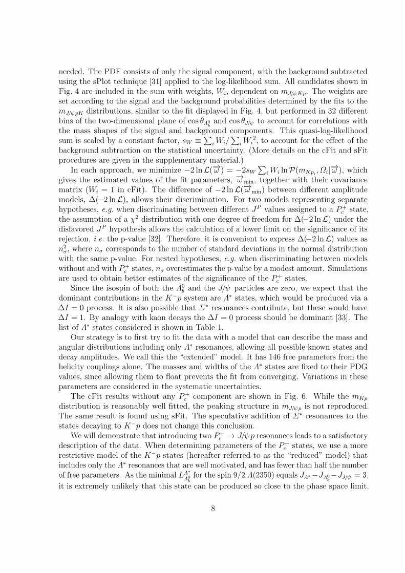
The cFit results without any P+c component are shown in Fig. 6. While the mKp

distribution is reasonably well fitted, the peaking structure in mJ/ψp is not reproduced.The same result is found using sFit. The speculative addition of Σ∗ resonances to thestates decaying to K−p does not change this conclusion.

We will demonstrate that introducing two P+c → J/ψp resonances leads to a satisfactory

description of the data. When determining parameters of the P+c states, we use a more

restrictive model of the K−p states (hereafter referred to as the “reduced” model) thatincludes only the Λ∗ resonances that are well motivated, and has fewer than half the numberof free parameters. As the minimal LΛ

∗

Λ0b

for the spin 9/2 Λ(2350) equals JΛ∗−JΛ0b−JJ/ψ = 3,

it is extremely unlikely that this state can be produced so close to the phase space limit.

8

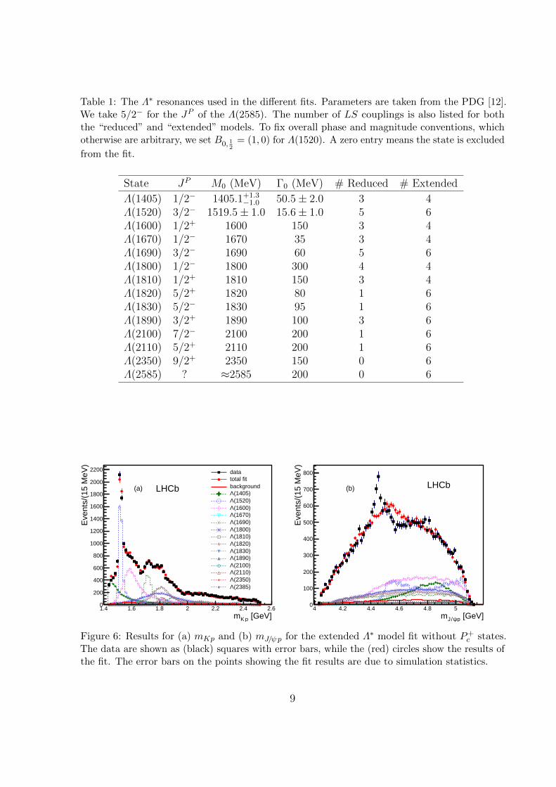
Table 1: The Λ∗ resonances used in the different fits. Parameters are taken from the PDG [12].We take 5/2− for the JP of the Λ(2585). The number of LS couplings is also listed for boththe “reduced” and “extended” models. To fix overall phase and magnitude conventions, whichotherwise are arbitrary, we set B0, 1

2= (1, 0) for Λ(1520). A zero entry means the state is excluded

from the fit.

State JP M0 (MeV) Γ0 (MeV) # Reduced # Extended

Λ(1405) 1/2− 1405.1+1.3−1.0 50.5± 2.0 3 4

Λ(1520) 3/2− 1519.5± 1.0 15.6± 1.0 5 6Λ(1600) 1/2+ 1600 150 3 4Λ(1670) 1/2− 1670 35 3 4Λ(1690) 3/2− 1690 60 5 6Λ(1800) 1/2− 1800 300 4 4Λ(1810) 1/2+ 1810 150 3 4Λ(1820) 5/2+ 1820 80 1 6Λ(1830) 5/2− 1830 95 1 6Λ(1890) 3/2+ 1890 100 3 6Λ(2100) 7/2− 2100 200 1 6Λ(2110) 5/2+ 2110 200 1 6Λ(2350) 9/2+ 2350 150 0 6Λ(2585) ? ≈2585 200 0 6

[GeV]pKm1.4 1.6 1.8 2 2.2 2.4 2.6

Eve

nts/

(15

MeV

)

0

200

400

600

800

1000

1200

1400

1600

1800

2000

2200

LHCb(a)

datatotal fitbackground

(1405)Λ(1520)Λ(1600)Λ(1670)Λ(1690)Λ(1800)Λ(1810)Λ(1820)Λ(1830)Λ(1890)Λ(2100)Λ(2110)Λ(2350)Λ(2385)Λ

[GeV]pψ/Jm4 4.2 4.4 4.6 4.8 5

Eve

nts/

(15

MeV

)

0

100

200

300

400

500

600

700

800

LHCb(b)

Figure 6: Results for (a) mKp and (b) mJ/ψp for the extended Λ∗ model fit without P+c states.

The data are shown as (black) squares with error bars, while the (red) circles show the results ofthe fit. The error bars on the points showing the fit results are due to simulation statistics.

9

In fact L = 3 is the highest orbital angular momentum observed, with a very small rate,in decays of B mesons [34] with much larger phase space available (Q = 2366 MeV, whilehere Q = 173 MeV), and without additional suppression from the spin counting factors

present in Λ(2350) production (all three ~JΛ∗ , ~JΛ0b

and ~JJ/ψ vectors have to line up in the

same direction to produce the minimal LΛ∗

Λ0b

value). Therefore, we eliminate it from the

reduced Λ∗ model. We also eliminate the Λ(2585) state, which peaks beyond the kinematiclimit and has unknown spin. The other resonances are kept but high LΛ

∗

Λ0b

amplitudes are

removed; only the lowest values are kept for the high mass resonances, with a smallerreduction for the lighter ones. The number of LS amplitudes used for each resonance islisted in Table 1. With this model we reduce the number of parameters needed to describethe Λ∗ decays from 146 to 64. For the different combinations of P+

c resonances that wetry, there are up to 20 additional free parameters. Using the extended model includingone resonant P+

c improves the fit quality, but it is still unacceptable (see supplementarymaterial). We find acceptable fits with two P+

c states. We use the reduced Λ∗ model forthe central values of our results. The differences in fitted quantities with the extendedmodel are included in the systematic uncertainties.

The best fit combination finds two P+c states with JP values of 3/2− and 5/2+, for the

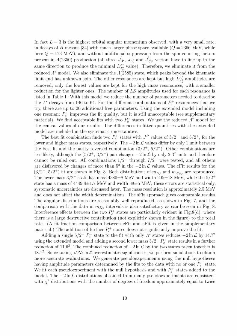
lower and higher mass states, respectively. The −2 lnL values differ by only 1 unit betweenthe best fit and the parity reversed combination (3/2+, 5/2−). Other combinations areless likely, although the (5/2+, 3/2−) pair changes −2 lnL by only 2.32 units and thereforecannot be ruled out. All combinations 1/2± through 7/2± were tested, and all othersare disfavored by changes of more than 52 in the −2 lnL values. The cFit results for the(3/2−, 5/2+) fit are shown in Fig. 3. Both distributions of mKp and mJ/ψp are reproduced.The lower mass 3/2− state has mass 4380±8 MeV and width 205±18 MeV, while the 5/2+

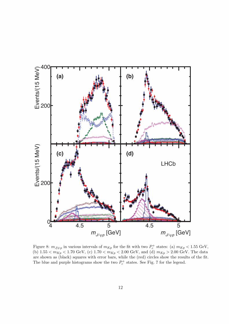
state has a mass of 4449.8±1.7 MeV and width 39±5 MeV; these errors are statistical only,systematic uncertainties are discussed later. The mass resolution is approximately 2.5 MeVand does not affect the width determinations. The sFit approach gives comparable results.The angular distributions are reasonably well reproduced, as shown in Fig. 7, and thecomparison with the data in mKp intervals is also satisfactory as can be seen in Fig. 8.Interference effects between the two P+

c states are particularly evident in Fig.8(d), wherethere is a large destructive contribution (not explicitly shown in the figure) to the totalrate. (A fit fraction comparison between cFit and sFit is given in the supplementarymaterial.) The addition of further P+

c states does not significantly improve the fit.Adding a single 5/2+ P+

c state to the fit with only Λ∗ states reduces −2 lnL by 14.72

using the extended model and adding a second lower mass 3/2− P+c state results in a further

reduction of 11.62. The combined reduction of −2 lnL by the two states taken together is18.72. Since taking

√∆2 lnL overestimates significances, we perform simulations to obtain

more accurate evaluations. We generate pseudoexperiments using the null hypotheseshaving amplitude parameters determined by the fits to the data with no or one P+

c state.We fit each pseudoexperiment with the null hypothesis and with P+

c states added to themodel. The −2 lnL distributions obtained from many pseudoexperiments are consistentwith χ2 distributions with the number of degrees of freedom approximately equal to twice

10

θcos1− 0.5− 0 0.5 10

500

1000

1500

2000

2500

0bΛθcos

[rad]φ2− 0 2

0

500

1000

1500

2000

2500

Kφ

θcos1− 0.5− 0 0.5 10

500

1000

1500

2000

2500

*Λθcos

[rad]φ2− 0 2

0

500

1000

1500

2000

2500

LHCb

datatotal fitbackground

(4450)cP(4380)cP(1405)Λ(1520)Λ(1600)Λ

(1670)Λ(1690)Λ(1800)Λ(1810)Λ(1820)Λ(1830)Λ(1890)Λ(2100)Λ(2110)Λ

θcos1− 0.5− 0 0.5 10

500

1000

1500

2000

2500

ψJ/θcos

[rad]φ2− 0 2

0

500

1000

1500

2000

2500

µφ

Figure 7: Various decay angular distributions for the fit with two P+c states. The data are shown

as (black) squares, while the (red) circles show the results of the fit. Each fit component is alsoshown. The angles are defined in the text.

11

Eve

nts/

(15

MeV

)

0

200

400

(a) (b)

[GeV]pψJ/m4 4.5 5

Eve

nts/

(15

MeV

)

0

200

400 (c)

[GeV]pψJ/m4 4.5 5

(d)

LHCb

Figure 8: mJ/ψp in various intervals of mKp for the fit with two P+c states: (a) mKp < 1.55 GeV,

(b) 1.55 < mKp < 1.70 GeV, (c) 1.70 < mKp < 2.00 GeV, and (d) mKp > 2.00 GeV. The dataare shown as (black) squares with error bars, while the (red) circles show the results of the fit.The blue and purple histograms show the two P+

c states. See Fig. 7 for the legend.

12

the number of extra parameters in the fit. Comparing these distributions with the ∆2 lnLvalues from the fits to the data, p-values can be calculated. These studies show reductionof the significances relative to

√∆2 lnL by about 20%, giving overall significances of 9σ

and 12σ, for the lower and higher mass P+c states, respectively. The combined significance

of two P+c states is 15σ. Use of the extended model to evaluate the significance includes

the effect of systematic uncertainties due to the possible presence of additional Λ∗ statesor higher L amplitudes.

Systematic uncertainties are evaluated for the masses, widths and fit fractions of theP+c states, and for the fit fractions of the two lightest and most significant Λ∗ states.

Additional sources of modeling uncertainty that we have not considered may affect thefit fractions of the heavier Λ∗ states. The sources of systematic uncertainties are listedin Table 2. They include differences between the results of the extended versus reducedmodel, varying the Λ∗ masses and widths, uncertainties in the identification requirementsfor the proton, and restricting its momentum, inclusion of a nonresonant amplitude inthe fit, use of separate higher and lower Λ0

b mass sidebands, alternate JP fits, varyingthe Blatt-Weisskopf barrier factor, d, between 1.5 and 4.5 GeV−1, changing the angularmomentum L used in Eq. (5) by one or two units, and accounting for potential mismodelingof the efficiencies. For the Λ(1405) fit fraction we also added an uncertainty for the Flattecouplings, determined by both halving and doubling their ratio, and taking the maximumdeviation as the uncertainty.

The stability of the results is cross-checked by comparing the data recorded in 2011/2012,with the LHCb dipole magnet polarity in up/down configurations, Λ0

b/Λ0b decays, and Λ0

b

produced with low/high values of pT. Extended model fits without including P+c states

were tried with the addition of two high mass Λ∗ resonances of freely varied mass andwidth, or four nonresonant components up to spin 3/2; these do not explain the data. Thefitters were tested on simulated pseudoexperiments and no biases were found. In addition,selection requirements are varied, and the vetoes of B0

s and B0 are removed and explicitmodels of those backgrounds added to the fit; all give consistent results.

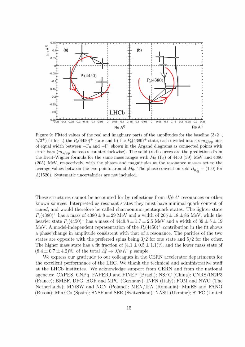
Further evidence for the resonant character of the higher mass, narrower, P+c state is

obtained by viewing the evolution of the complex amplitude in the Argand diagram [12].In the amplitude fits discussed above, the Pc(4450)+ is represented by a Breit-Wigneramplitude, where the magnitude and phase vary with mJ/ψp according to an approximatelycircular trajectory in the (ReAPc , ImAPc) plane, where APc is the mJ/ψp dependentpart of the Pc(4450)+ amplitude. We perform an additional fit to the data using thereduced Λ∗ model, in which we represent the Pc(4450)+ amplitude as the combination ofindependent complex amplitudes at six equidistant points in the range ±Γ0 = 39 MeVaround M0 = 4449.8 MeV as determined in the default fit. Real and imaginary parts ofthe amplitude are interpolated in mass between the fitted points. The resulting Arganddiagram, shown in Fig. 9(a), is consistent with a rapid counter-clockwise change of thePc(4450)+ phase when its magnitude reaches the maximum, a behavior characteristic ofa resonance. A similar study for the wider state is shown in Fig. 9(b); although the fitdoes show a large phase change, the amplitude values are sensitive to the details of the Λ∗

model and so this latter study is not conclusive.

13

Different binding mechanisms of pentaquark states are possible. Tight-binding wasenvisioned originally [3,4,35]. A possible explanation is heavy-light diquarks [36]. Examplesof other mechanisms include a diquark-diquark-antiquark model [37,38], a diquark-triquarkmodel [39], and a coupled channel model [40]. Weakly bound “molecules” of a baryon plusa meson have been also discussed [41].

Models involving thresholds or “cusps” have been invoked to explain some exotic mesoncandidates via nonresonant scattering mechanisms [42–44]. There are certain obviousdifficulties with the use of this approach to explain our results. The closest threshold tothe high mass state is at 4457.1±0.3 MeV resulting from a Λc(2595)+D0 combination,which is somewhat higher than the peak mass value and would produce a structure withquantum numbers JP = 1/2+ which are disfavored by our data. There is no thresholdclose to the lower mass state.

In conclusion, we have presented a full amplitude fit to the Λ0b → J/ψK−p decay.

We observe significant Λ∗ production recoiling against the J/ψ with the lowest masscontributions, the Λ(1405) and Λ(1520) states having fit fractions of (15± 1± 6)% and(19±1±4)%, respectively. The data cannot be satisfactorily described without including twoBreit-Wigner shaped resonances in the J/ψp invariant mass distribution. The significancesof the lower mass and higher mass states are 9 and 12 standard deviations, respectively.

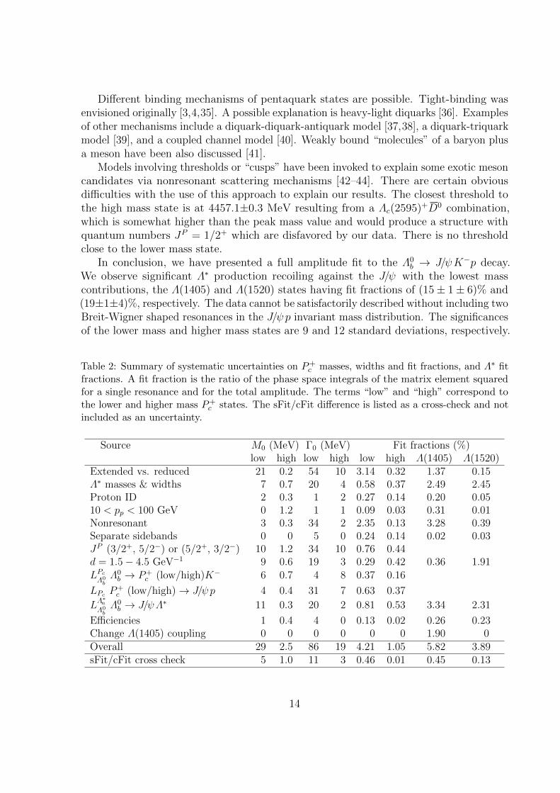
Table 2: Summary of systematic uncertainties on P+c masses, widths and fit fractions, and Λ∗ fit

fractions. A fit fraction is the ratio of the phase space integrals of the matrix element squaredfor a single resonance and for the total amplitude. The terms “low” and “high” correspond tothe lower and higher mass P+

c states. The sFit/cFit difference is listed as a cross-check and notincluded as an uncertainty.

Source M0 (MeV) Γ0 (MeV) Fit fractions (%)low high low high low high Λ(1405) Λ(1520)

Extended vs. reduced 21 0.2 54 10 3.14 0.32 1.37 0.15Λ∗ masses & widths 7 0.7 20 4 0.58 0.37 2.49 2.45Proton ID 2 0.3 1 2 0.27 0.14 0.20 0.0510 < pp < 100 GeV 0 1.2 1 1 0.09 0.03 0.31 0.01Nonresonant 3 0.3 34 2 2.35 0.13 3.28 0.39Separate sidebands 0 0 5 0 0.24 0.14 0.02 0.03JP (3/2+, 5/2−) or (5/2+, 3/2−) 10 1.2 34 10 0.76 0.44d = 1.5− 4.5 GeV−1 9 0.6 19 3 0.29 0.42 0.36 1.91LPcΛ0bΛ0b → P+

c (low/high)K− 6 0.7 4 8 0.37 0.16

LPc P+c (low/high)→ J/ψp 4 0.4 31 7 0.63 0.37

LΛ∗nΛ0bΛ0b → J/ψΛ∗ 11 0.3 20 2 0.81 0.53 3.34 2.31

Efficiencies 1 0.4 4 0 0.13 0.02 0.26 0.23Change Λ(1405) coupling 0 0 0 0 0 0 1.90 0Overall 29 2.5 86 19 4.21 1.05 5.82 3.89sFit/cFit cross check 5 1.0 11 3 0.46 0.01 0.45 0.13

14

Re A

-0.35 -0.3 -0.25 -0.2 -0.15 -0.1 -0.05 0 0.05 0.1 0.1

-0.35

-0.3

-0.25

-0.2

-0.15

-0.1

-0.05

0

0.05

0.1

0.15

LHCb

(4450)cP

(a)

15 -0.1 -0.05 0 0.05 0.1 0.15 0.2 0.25 0.3 0.35

(4380)cP

(b)

Pc Re APc

Im A

P c

Figure 9: Fitted values of the real and imaginary parts of the amplitudes for the baseline (3/2−,5/2+) fit for a) the Pc(4450)+ state and b) the Pc(4380)+ state, each divided into six mJ/ψp binsof equal width between −Γ0 and +Γ0 shown in the Argand diagrams as connected points witherror bars (mJ/ψp increases counterclockwise). The solid (red) curves are the predictions fromthe Breit-Wigner formula for the same mass ranges with M0 (Γ0) of 4450 (39) MeV and 4380(205) MeV, respectively, with the phases and magnitudes at the resonance masses set to theaverage values between the two points around M0. The phase convention sets B0, 1

2= (1, 0) for

Λ(1520). Systematic uncertainties are not included.

These structures cannot be accounted for by reflections from J/ψΛ∗ resonances or otherknown sources. Interpreted as resonant states they must have minimal quark content ofccuud, and would therefore be called charmonium-pentaquark states. The lighter statePc(4380)+ has a mass of 4380± 8± 29 MeV and a width of 205± 18± 86 MeV, while theheavier state Pc(4450)+ has a mass of 4449.8± 1.7± 2.5 MeV and a width of 39± 5± 19MeV. A model-independent representation of the Pc(4450)+ contribution in the fit showsa phase change in amplitude consistent with that of a resonance. The parities of the twostates are opposite with the preferred spins being 3/2 for one state and 5/2 for the other.The higher mass state has a fit fraction of (4.1± 0.5± 1.1)%, and the lower mass state of(8.4± 0.7± 4.2)%, of the total Λ0

b → J/ψK−p sample.We express our gratitude to our colleagues in the CERN accelerator departments for

the excellent performance of the LHC. We thank the technical and administrative staffat the LHCb institutes. We acknowledge support from CERN and from the nationalagencies: CAPES, CNPq, FAPERJ and FINEP (Brazil); NSFC (China); CNRS/IN2P3(France); BMBF, DFG, HGF and MPG (Germany); INFN (Italy); FOM and NWO (TheNetherlands); MNiSW and NCN (Poland); MEN/IFA (Romania); MinES and FANO(Russia); MinECo (Spain); SNSF and SER (Switzerland); NASU (Ukraine); STFC (United

15

Kingdom); NSF (USA). The Tier1 computing centres are supported by IN2P3 (France),KIT and BMBF (Germany), INFN (Italy), NWO and SURF (The Netherlands), PIC(Spain), GridPP (United Kingdom). We are indebted to the communities behind themultiple open source software packages on which we depend. We are also thankful forthe computing resources and the access to software R&D tools provided by Yandex LLC(Russia). Individual groups or members have received support from EPLANET, MarieSk lodowska-Curie Actions and ERC (European Union), Conseil general de Haute-Savoie,Labex ENIGMASS and OCEVU, Region Auvergne (France), RFBR (Russia), XuntaGaland GENCAT (Spain), Royal Society and Royal Commission for the Exhibition of 1851(United Kingdom).

16

Appendix: Supplementary material

Contents

1 Variables used in the BDTG 18

2 Additional fit results 182.1 Reduced model fit projections for mJ/ψK− . . . . . . . . . . . . . . . . . . 182.2 Reduced model angular fits with two P+

c states for m(K−p) > 2 GeV . . . 192.3 Extended model fit with one P+

c state . . . . . . . . . . . . . . . . . . . . 212.4 Results of extended model fit with two Pc

+ states . . . . . . . . . . . . . . 21

3 Fit fraction comparison between cFit and sFit 21

4 Details of the matrix element for the decay amplitude 234.1 Helicity formalism and notation . . . . . . . . . . . . . . . . . . . . . . . . 234.2 Matrix element for the Λ∗ decay chain . . . . . . . . . . . . . . . . . . . . 274.3 Matrix element for the P+

c decay chain . . . . . . . . . . . . . . . . . . . . 314.4 Reduction of the number of helicity couplings . . . . . . . . . . . . . . . . 36

5 Details of fitting techniques 37

17

1 Variables used in the BDTG

Muon identification uses information from several parts of the detector, including theRICH detectors, the calorimeters and the muon system. Likelihoods are formed for themuon and pion hypotheses. The difference in the logarithms of the likelihoods, DLL(µ−π),is used to distinguish between the two [16]. The smaller value of the two discriminantsDLL(µ+ − π+) and DLL(µ− − π−) is used as one of the BDTG variables.

The next set of variables uses the kaon and proton tracks. The χ2IP is defined as the

difference in χ2 of the primary vertex reconstructed with and without the considered track.The smaller χ2

IP of the K− and p is used in the BDTG. The scalar pT sum of the K− andp is another variable.

The last set of variables uses the Λ0b candidate. The cosine of the angle between a

vector from the primary vertex to the Λ0b vertex and the Λ0

b momentum vector is oneinput variable. In addition the χ2

IP, the flight distance, the pT and the vertex χ2 of the Λ0b

candidate are used.

2 Additional fit results

2.1 Reduced model fit projections for mJ/ψK

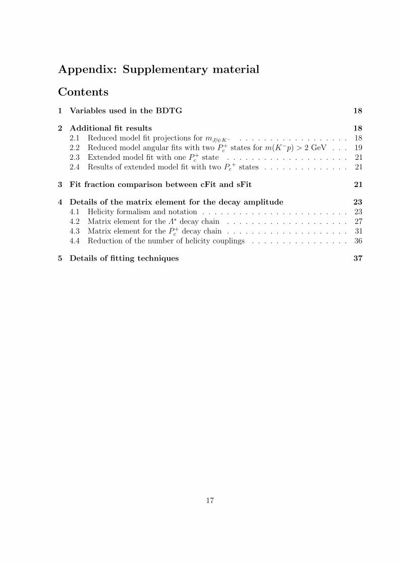
The Dalitz plots for the other two possible projections are shown in Fig. 10. There is noobvious resonance structure in the J/ψK− mass-squared distribution.

Our fit describes well the mJ/ψK distribution as shown by viewing the projections ofthe reduced model fit. They are shown for different slices of mKp in Fig. 11.

]2 [GeVpψJ/2m

20 25

]2 [G

eVK

ψJ/2

m

13141516171819202122 (a)

LHCb

]2 [GeVKp2m

2 3 4 5 6

]2 [G

eVK

ψJ/2

m

13141516171819202122 (b)LHCb

Figure 10: (a) Invariant mass squared of J/ψK− versus J/ψp and (b) of J/ψK− versus K−p forcandidates within ±15 MeV of the Λ0

b mass.

18

[GeV]KψJ/m4 4.5

Eve

nts/

(15

MeV

)

0

200

(a)

[GeV]KψJ/m4 4.5

Eve

nts/

(15

MeV

)

0

200

(b)

[GeV]KψJ/m4 4.5

Eve

nts/

(15

MeV

)

0

200

(c)

[GeV]KψJ/m4 4.5

Eve

nts/

(15

MeV

)

0

200

LHCb

(d)

[GeV]KψJ/m4 4.5

Eve

nts/

(15

MeV

)

0

500(e)

[GeV]KψJ/m4 4.5

Eve

nts/

(15

MeV

)

0

500

datatotal fitbackground

(4450)cP(4380)cP(1405)Λ(1520)Λ(1600)Λ

(1670)Λ(1690)Λ(1800)Λ(1810)Λ(1820)Λ(1830)Λ(1890)Λ(2100)Λ(2110)Λ

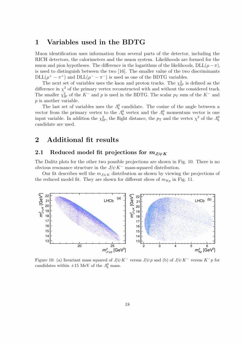
Figure 11: Projections onto mJ/ψK in various intervals of mKp for the reduced model fit (cFit) with

two P+c states of JP equal to 3/2− and 5/2+: (a) mKp < 1.55 GeV, (b) 1.55 < mKp < 1.70 GeV,

(c) 1.70 < mKp < 2.00 GeV, (d) mKp > 2.00 GeV, and (e) all mKp. The data are shown as(black) squares with error bars, while the (red) circles show the results of the fit. The individualresonances are given in the legend.

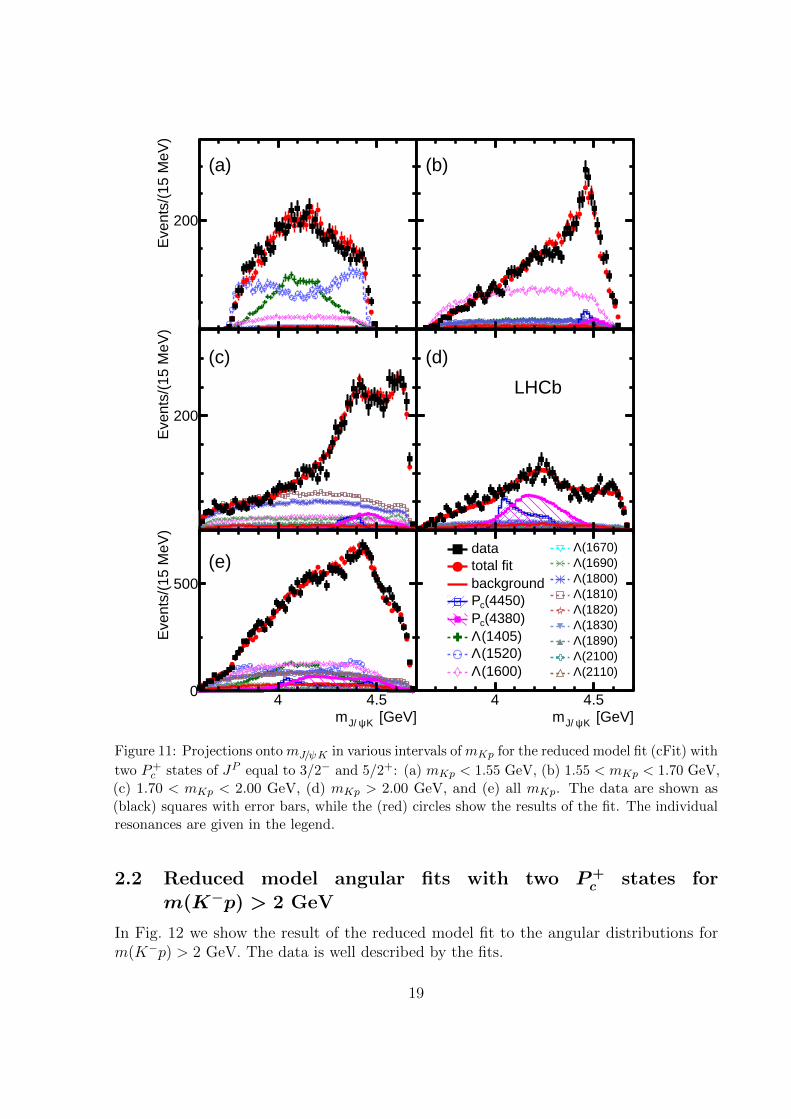
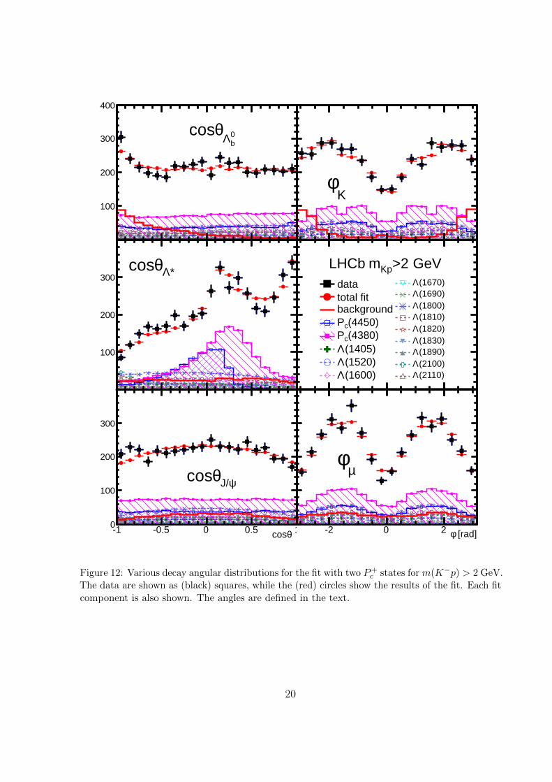
2.2 Reduced model angular fits with two P+c states for

m(K−p) > 2 GeV

In Fig. 12 we show the result of the reduced model fit to the angular distributions form(K−p) > 2 GeV. The data is well described by the fits.

19

θcos-1 -0.5 0 0.5 10

100

200

300

400

0bΛθcos

[rad]φ-2 0 2

0

100

200

300

400

Kφ

θcos-1 -0.5 0 0.5 10

100

200

300

400

*Λθcos

[rad]φ-2 0 2

0

100

200

300

400

GeV>2KpmLHCb datatotal fitbackground

(4450)cP(4380)cP(1405)Λ(1520)Λ(1600)Λ

(1670)Λ(1690)Λ(1800)Λ(1810)Λ(1820)Λ(1830)Λ(1890)Λ(2100)Λ(2110)Λ

θcos-1 -0.5 0 0.5 10

100

200

300

400

ψJ/θcos

[rad]φ-2 0 2

0

100

200

300

400

µφ

Figure 12: Various decay angular distributions for the fit with two P+c states for m(K−p) > 2 GeV.

The data are shown as (black) squares, while the (red) circles show the results of the fit. Each fitcomponent is also shown. The angles are defined in the text.

20

[GeV]pKm1.4 1.6 1.8 2 2.2 2.4 2.6

Eve

nts/

(15

MeV

)

0

200

400

600

800

1000

1200

1400

1600

1800

2000

2200

LHCb(a)

datatotal fitbackground

cP(1405)Λ(1520)Λ(1600)Λ(1670)Λ(1690)Λ(1800)Λ(1810)Λ(1820)Λ(1830)Λ(1890)Λ(2100)Λ(2110)Λ(2350)Λ(2385)Λ

[GeV]pψ/Jm4 4.2 4.4 4.6 4.8 5

Eve

nts/

(15

MeV

)

0

100

200

300

400

500

600

700

800

LHCb(b)

Figure 13: Results of the fit with one JP = 5/2+ P+c candidate. (a) Projection of the invariant

mass of K−p combinations from Λ0b → J/ψK−p candidates. The data are shown as (black)

squares with error bars, while the (red) circles show the results of the fit; (b) the correspondingJ/ψp mass projection. The (blue) shaded plot shows the P+

c projection, the other curves representindividual Λ∗ states.

2.3 Extended model fit with one P+c

In the fits with one P+c amplitude, we test JP values of 1/2±, 3/2± and 5/2±. The mass

and width of the putative P+c state are allowed to vary. There are a total of 146 free

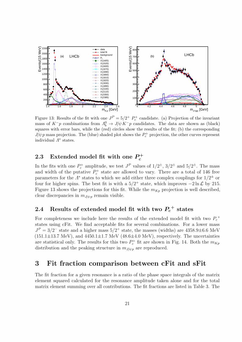
parameters for the Λ∗ states to which we add either three complex couplings for 1/2± orfour for higher spins. The best fit is with a 5/2+ state, which improves −2 lnL by 215.Figure 13 shows the projections for this fit. While the mKp projection is well described,clear discrepancies in mJ/ψp remain visible.

2.4 Results of extended model fit with two Pc+ states

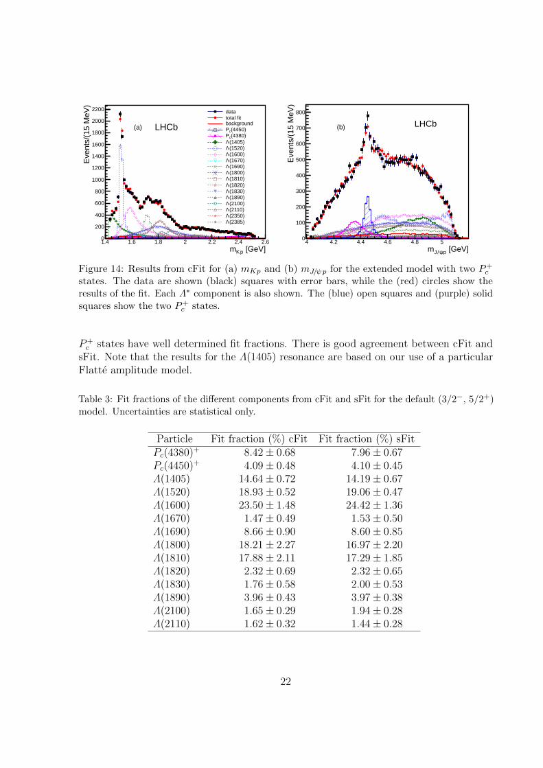
For completeness we include here the results of the extended model fit with two Pc+

states using cFit. We find acceptable fits for several combinations. For a lower massJP = 3/2− state and a higher mass 5/2+ state, the masses (widths) are 4358.9±6.6 MeV(151.1±13.7 MeV), and 4450.1±1.7 MeV (48.6±4.0 MeV), respectively. The uncertaintiesare statistical only. The results for this two P+

c fit are shown in Fig. 14. Both the mKp

distribution and the peaking structure in mJ/ψp are reproduced.

3 Fit fraction comparison between cFit and sFit

The fit fraction for a given resonance is a ratio of the phase space integrals of the matrixelement squared calculated for the resonance amplitude taken alone and for the totalmatrix element summing over all contributions. The fit fractions are listed in Table 3. The

21

[GeV]pKm1.4 1.6 1.8 2 2.2 2.4 2.6

Eve

nts/

(15

MeV

)

0

200

400

600

800

1000

1200

1400

1600

1800

2000

2200

LHCb(a)

datatotal fitbackground

(4450)cP(4380)cP(1405)Λ(1520)Λ(1600)Λ(1670)Λ(1690)Λ(1800)Λ(1810)Λ(1820)Λ(1830)Λ(1890)Λ(2100)Λ(2110)Λ(2350)Λ(2385)Λ

[GeV]pψ/Jm4 4.2 4.4 4.6 4.8 5

Eve

nts/

(15

MeV

)

0

100

200

300

400

500

600

700

800

LHCb(b)

Figure 14: Results from cFit for (a) mKp and (b) mJ/ψp for the extended model with two P+c

states. The data are shown (black) squares with error bars, while the (red) circles show theresults of the fit. Each Λ∗ component is also shown. The (blue) open squares and (purple) solidsquares show the two P+

c states.

P+c states have well determined fit fractions. There is good agreement between cFit and

sFit. Note that the results for the Λ(1405) resonance are based on our use of a particularFlatte amplitude model.

Table 3: Fit fractions of the different components from cFit and sFit for the default (3/2−, 5/2+)model. Uncertainties are statistical only.

Particle Fit fraction (%) cFit Fit fraction (%) sFitPc(4380)+ 8.42± 0.68 7.96± 0.67Pc(4450)+ 4.09± 0.48 4.10± 0.45Λ(1405) 14.64± 0.72 14.19± 0.67Λ(1520) 18.93± 0.52 19.06± 0.47Λ(1600) 23.50± 1.48 24.42± 1.36Λ(1670) 1.47± 0.49 1.53± 0.50Λ(1690) 8.66± 0.90 8.60± 0.85Λ(1800) 18.21± 2.27 16.97± 2.20Λ(1810) 17.88± 2.11 17.29± 1.85Λ(1820) 2.32± 0.69 2.32± 0.65Λ(1830) 1.76± 0.58 2.00± 0.53Λ(1890) 3.96± 0.43 3.97± 0.38Λ(2100) 1.65± 0.29 1.94± 0.28Λ(2110) 1.62± 0.32 1.44± 0.28

22

4 Details of the matrix element for the decay ampli-

tude

The matrix element for Λ0b → ψK−p, ψ → µ+µ− decays2 must allow for various conven-

tional Λ∗ → K−p resonances and exotic pentaquark states P+c → ψp that could interfere

with each other.We use the helicity formalism to write down the matrix element. To make the derivation

of the matrix element easier to comprehend we start with a brief outline of this formalismand our notation. Then we discuss the application to the Λ0

b → Λ∗ψ, Λ∗ → K−p,ψ → µ+µ− decay sequence, called hereafter the Λ∗ decay chain matrix element. Next wediscuss construction of the Λ0

b → P+c K

−, P+c → ψp, ψ → µ+µ− decay sequence, called

hereafter the Pc decay chain matrix element, which can be coherently added to that for theΛ∗ decay chain. We also discuss a possible reduction of the number of helicity couplingsto be determined from the data using their relationships to the LS couplings.

4.1 Helicity formalism and notation

For each two-body decay A→ B C, a coordinate system is set up in the rest frame of A,with z being3 the direction of quantization for its spin. We denote this coordinate systemas (x

A0 , y

A0 , z

A0 ), where the superscript “A” means “in the rest frame of A”, while

the subscript “0” means the initial coordinates. For the first particle in the decay chain(Λ0

b), the choice of these coordinates is arbitrary.4 However, once defined, these coordinatesmust be used consistently between all decay sequences described by the matrix element.For subsequent decays, e.g. B → DE, the choice of these coordinates is already fixed bythe transformation from the A to the B rest frames, as discussed below. Helicity is definedas the projection of the spin of the particle onto the direction of its momentum. Whenthe z axis coincides with the particle momentum, we denote its spin projection onto it(i.e. the mz quantum number) as λ. To use the helicity formalism, the initial coordinatesystem must be rotated to align the z axis with the direction of the momentum of one ofthe daughter particles, e.g. the B. A generalized rotation operator can be formulated inthree-dimensional space, R(α, β, γ), that uses Euler angles. Applying this operator resultsin a sequence of rotations: first by the angle α about the z0 axis, followed by the angle βabout the rotated y1 axis and then finally by the angle γ about the rotated z2 axis. We usea subscript denoting the axes, to specify the rotations which have been already performedon the coordinates. The spin eigenstates of particle A, |JA,mA〉, in the (x

A0 , y

A0 , z

A0 )

coordinate system can be expressed in the basis of its spin eigenstates, |JA,m′A〉, in the

2We denote J/ψ as ψ for efficiency of the notation.3The “hat” symbol denotes a unit vector in a given direction.4When designing an analysis to be sensitive (or insensitive) to a particular case of polarization, the

choice is not arbitrary, but this does not change the fact that one can quantize the Λ0b spin along any

well-defined direction. The Λ0b polarization may be different for different choices.

23

rotated (xA

3 , yA

3 , zA

3 ) coordinate system with the help of Wigner’s D−matrices

|JA,mA〉 =∑m′A

D JAmA,m

′A

(α, β, γ)∗ |JA,m′A〉, (9)

whereD Jm,m′(α, β, γ)∗ = 〈J,m|R(α, β, γ)|J,m′〉∗ = eimα d Jm,m′(β) eim

′γ, (10)

and where the small-d Wigner matrix contains known functions of β that depend onJ,m,m′. To achieve the rotation of the original z

A0 axis onto the B momentum (~p

AB ),

it is sufficient to rotate by α = φAB , β = θ

AB , where φ

AB , θ

AB are the azimuthal and

polar angles of the B momentum vector in the original coordinates i.e. (xA

0 , yA

0 , zA

0 ).This is depicted in Fig. 15, for the case when the quantization axis for the spin of A is itsmomentum in some other reference frame. Since the third rotation is not necessary, weset γ = 0.5 The angle θ

AB is usually called “the A helicity angle”, thus to simplify the

notation we will denote it as θA. For compact notation, we will also denote φAB as φB.

These angles can be determined from6

φB = atan2(pAB y, p

AB x

)= atan2

(yA

0 · ~p AB , xA

0 · ~p AB

)= atan2

((zA

0 × x A0 ) · ~p AB , xA

0 · ~p AB

), (11)

cos θA = zA

0 · p AB . (12)

Angular momentum conservation requires m′A = m′B+m′C = λB−λC (since ~pAC points

in the opposite direction to zA

3 , m′C = −λC). Each two-body decay adds a multiplicativeterm to the matrix element

HA→BCλB , λC

D JAmA, λB−λC (φB, θA, 0)∗. (13)

The helicity couplings HA→BCλB , λC

are complex constants. Their products from subsequentdecays are to be determined by the fit to the data (they represent the decay dynamics). Ifthe decay is strong or electromagnetic, it conserves parity which reduces the number ofindependent helicity couplings via the relation

HA→BC−λB ,−λC = PA PB PC (−1)JB+JC−JAHA→BC

λB , λC, (14)

where P stands for the intrinsic parity of a particle.

5An alternate convention is to set γ = −α. The two conventions lead to equivalent formulae.6The function atan2(x, y) is the tan−1(y/x) function with two arguments. The purpose of using

two arguments instead of one is to gather information on the signs of the inputs in order to return theappropriate quadrant of the computed angle.

24

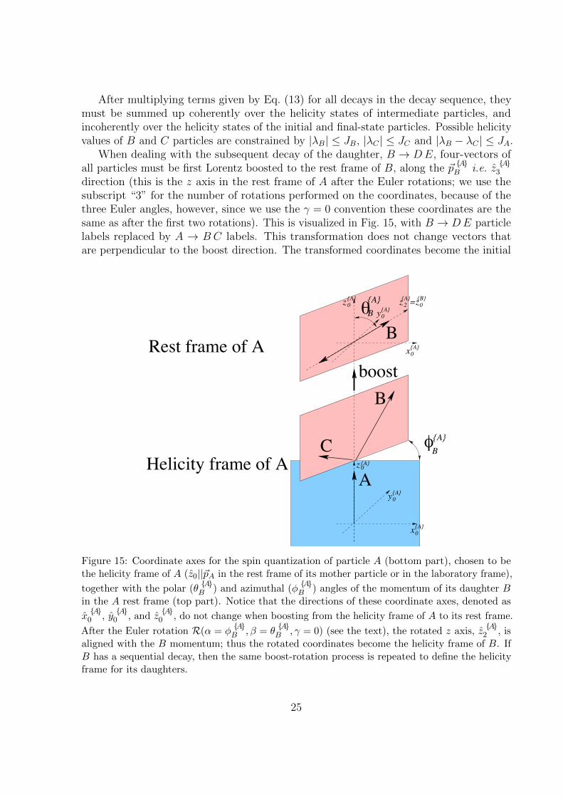
After multiplying terms given by Eq. (13) for all decays in the decay sequence, theymust be summed up coherently over the helicity states of intermediate particles, andincoherently over the helicity states of the initial and final-state particles. Possible helicityvalues of B and C particles are constrained by |λB| ≤ JB, |λC | ≤ JC and |λB − λC | ≤ JA.

When dealing with the subsequent decay of the daughter, B → DE, four-vectors ofall particles must be first Lorentz boosted to the rest frame of B, along the ~p

AB i.e. z

A3

direction (this is the z axis in the rest frame of A after the Euler rotations; we use thesubscript “3” for the number of rotations performed on the coordinates, because of thethree Euler angles, however, since we use the γ = 0 convention these coordinates are thesame as after the first two rotations). This is visualized in Fig. 15, with B → DE particlelabels replaced by A → B C labels. This transformation does not change vectors thatare perpendicular to the boost direction. The transformed coordinates become the initial

x

C x

y

z

A

A B

0A

A

Rest frame of A

Helicity frame of A 0

0

0

φ A

boost

2

C

B

z A0

0

A

A

A

B

θBA z =z

0

By

Figure 15: Coordinate axes for the spin quantization of particle A (bottom part), chosen to bethe helicity frame of A (z0||~pA in the rest frame of its mother particle or in the laboratory frame),

together with the polar (θAB ) and azimuthal (φ

AB ) angles of the momentum of its daughter B

in the A rest frame (top part). Notice that the directions of these coordinate axes, denoted as

xA

0 , yA

0 , and zA

0 , do not change when boosting from the helicity frame of A to its rest frame.

After the Euler rotation R(α = φAB , β = θ

AB , γ = 0) (see the text), the rotated z axis, z

A2 , is

aligned with the B momentum; thus the rotated coordinates become the helicity frame of B. IfB has a sequential decay, then the same boost-rotation process is repeated to define the helicityframe for its daughters.

25

coordinate system quantizing the spin of B in its rest frame,

xB

0 = xA

3 ,

yB

0 = yA

3 ,

zB

0 = zA

3 . (15)

The processes of rotation and subsequent boosting can be repeated until the final-stateparticles are reached. In practice, there are two equivalent ways to determine the z

B0

direction. Using Eq. (15) we can set it to the direction of the B momentum in the A restframe

zB

0 = zA

3 = pAB . (16)

Alternatively, we can make use of the fact that B and C are back-to-back in the rest frameof A, ~p

AC = −~p AB . Since the momentum of C is antiparallel to the boost direction from

the A to B rest frames, the C momentum in the B rest frame will be different, but it willstill be antiparallel to this boost direction

zB

0 = −p BC . (17)

To determine xB

0 from Eq. (15), we need to find xA

3 . After the first rotation by φBabout z

A0 , the x

A1 axis is along the component of ~p

AB which is perpendicular to the

zA

0 axis

~aAB⊥z0 ≡ (~p

AB )⊥z A0

= ~pAB − (~p

AB )||z A0

,

= ~pAB − (~p

AB · z A0 ) z

A0 ,

xA

1 = aAB⊥z0 =

~aAB⊥z0

|~a AB⊥z0 |. (18)

After the second rotation by θA about yA

1 , zA

2 ≡ zA

3 = pAB , and x

A2 = x

A3 is

antiparallel to the component of the zA

0 vector that is perpendicular to the new z axis

i.e. pAB . Thus

~aAz0⊥B ≡ (z

A0 )⊥~p AB

= zA

0 − (zA

0 · p AB ) pAB ,

xB

0 = xA

3 = − aAz0⊥B = −

~aAz0⊥B

|~a Az0⊥B |. (19)

Then we obtain yB

0 = zB

0 × x B0 .If C also decays, C → F G, then the coordinates for the quantization of C spin in the

C rest frame are defined by

zC

0 = −z A3 = pAC = −p CB , (20)

xC

0 = xA

3 = − a Az0⊥B = +aAz0⊥C , (21)

yC

0 = zC

0 × x C0 , (22)

26

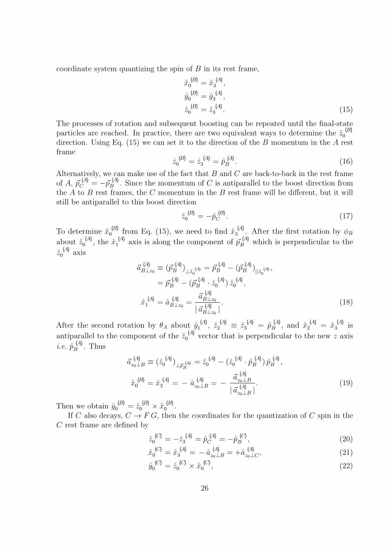
i.e. the z axis is reflected compared to the system used for the decay of particle B (it mustpoint in the direction of C momentum in the A rest frame), but the x axis is kept thesame, since we chose particle B for the rotation used in Eq. (13).

4.2 Matrix element for the Λ∗ decay chain

We first discuss the part of the matrix element describing conventional Λ0b → Λ∗nψ, Λ∗n → Kp

decays (i.e. Λ∗ decay chain), where Λ∗n denotes various possible excitations of the Λ, e.g.Λ(1520). For simplicity we often refer to Λ∗n as Λ∗, unless we label an n-dependent quantity.

The weak decay Λ0b → Λ∗nψ is described by

HΛ0b→Λ

∗nψ

λΛ∗ , λψD

12λΛ0b, λΛ∗−λψ(φΛ∗ , θΛ0

b, 0)∗, (23)

where HΛ0b→Λ

∗nψ

λΛ∗ , λψare resonance (i.e. n) dependent helicity couplings to be determined by a

fit to the data. There are 4 different complex values of these couplings to be determinedfor each Λ∗n resonance with spin JΛ∗n = 1

2, and 6 values for higher spins. The couplings are

complex parameters; thus each independent coupling contributes 2 free parameters (takento be real and imaginary parts) to the fit. Since the ψ and Λ∗ are intermediate particlesin the decay chain, the matrix element terms for different values of λψ and λΛ∗ must beadded coherently.

The choice of the zΛ0b

0 direction for the Λ0b spin quantization is arbitrary. We choose

the Λ0b momentum in the lab frame to define the z

Λ0b

0 direction, giving its spin projectiononto this axis the meaning of the Λ0

b helicity (λΛ0b). In the Λ0

b rest frame, this direction isdefined by the direction of the boost from the lab frame (Eq. (16)),

zΛ0b

0 = plabΛ0b, (24)

as depicted in Fig. 16. With this choice, θΛ0b

is the Λ0b helicity angle and can be calculated

ascos θΛ0

b= p

labΛ0b· p Λ

0b

Λ∗ . (25)

Longitudinal polarization of the Λ0b via strong production mechanisms is forbidden due to

parity conservation in strong interactions, causing λΛ0b

= +12

and −12

to be equally likely.

Terms with different λΛ0b

values must be added incoherently. The choice of xΛ0b

0 direction

in the Λ0b rest frame is also arbitrary. We use the Λ0

b → Λ∗ψ decay plane in the lab frameto define it, which makes the φΛ∗ angle zero by definition.

The strong decay Λ∗n → Kp is described by a term

HΛ∗n→Kpλp

DJΛ∗nλΛ∗ , λp

(φK , θΛ∗ , 0)∗ RΛ∗n (mKp). (26)

Since the K− meson is spinless, the resonance-dependent helicity couplingHΛ∗n→Kpλp

depends

only on proton helicity, λp = ±12. As strong decays conserve parity, the two helicity

couplings are related

HΛ∗n→Kp−λp = −PΛ∗n (−1)JΛ∗n−

12 HΛ∗n→Kp

λp, (27)

27

ΛΛ

μ

μ

μ

μ

ψ

ppKKθ θ φ

θ

*

+

−

+

−K − −

ψ Λ

Λ

b

*ψ *

φ = 0

Λ

Λ

φ μψ*

Λ

b

lab frame

rest frame0

0

rest frame

∗

x

z

b

Λ

rest frame

Figure 16: Definition of the decay angles in the Λ∗ decay chain.

where PΛ∗n is the parity of Λ∗n . Since the overall magnitude and phase of HΛ∗n→Kp+ 1

2

can

be absorbed into a redefinition of the HΛ0b→Λ

∗nψ

λΛ∗ , λψcouplings, we set HΛ∗n→Kp

+ 12

= (1, 0) and

HΛ∗n→Kp− 1

2

= (PΛ∗n (−1)JΛ∗n−32 , 0), where the values in parentheses give the real and imaginary

parts of the couplings.The angles φK and θΛ∗ are the azimuthal and polar angles of the kaon in the Λ∗ rest

frame (see Fig. 16). The zΛ∗

0 direction is defined by the boost direction from the Λ0b rest

frame, which coincides with the −~p Λ∗

ψ direction in this frame (Eq. (17)). This leads to

cos θΛ∗ = −p Λ∗

ψ · p Λ∗

K , (28)

with both vectors in the Λ∗ rest frame. As explained in Sec. 4.1, the xΛ∗

0 direction isdefined by the choice of coordinates in the Λ0

b rest frame discussed above. FollowingEq. (19) and (24), we have

~aΛ0b

z0⊥Λ∗ = plabΛ0b− (p

labΛ0b· p Λ

0b

Λ∗ ) pΛ0b

Λ∗ ,

xΛ∗

0 = xΛ0b

3 = −~aΛ0b

z0⊥Λ∗

|~a Λ0b

z0⊥Λ∗ |. (29)

The azimuthal angle of the K− can now be determined in the Λ∗ rest frame from (Eq. (11))

φK = atan2(−(p

Λ∗ψ × x Λ

∗0 ) · p Λ

∗K , x

Λ∗0 · p Λ

∗K

). (30)

The term RΛ∗n (mKp) describes the Λ∗n resonance that appears in the invariant mass

28

distribution of the kaon-proton system,

RΛ∗n (mKp) = B′LΛ∗nΛ0b

(p, p0, d)

(p

MΛ0b

)LΛ∗nΛ0b

BW(mKp|MΛ∗n0 ,Γ

Λ∗n0 )B′LΛ∗n

(q, q0, d)

(q

MΛ∗n0

)LΛ∗n

.

(31)

Here, p is the Λ∗ momentum in the Λ0b rest frame (p = |~p Λ

0b

Λ∗ |). Similarly, q is the K−

momentum in the Λ∗ rest frame (q = |~p Λ∗

K |). The symbols p0 and q0 denote values of

these quantities at the resonance peak (mKp = MΛ∗n0 ). The orbital angular momentum

between the Λ∗ and ψ particles in the Λ0b decay is denoted as L

Λ∗nΛ0b. Similarly, LΛ∗n is the

orbital angular momentum between the p and K− in the Λ∗n decay. For the orbital angularmomentum barrier factors, pLB′L(p, p0, d), we use the Blatt-Weisskopf functions [45],

B′0(p, p0, d) =1 ,

B′1(p, p0, d) =

√1 + (p0 d)2

1 + (p d)2,

B′2(p, p0, d) =

√9 + 3(p0 d)2 + (p0 d)4

9 + 3(p d)2 + (p d)4, (32)

B′3(p, p0, d) =

√225 + 45(p0 d)2 + 6(p0 d)4 + (p0 d)6

225 + 45(p d)2 + 6(p d)4 + (p d)6,

B′4(p, p0, d) =

√11025 + 1575(p0 d)2 + 135(p0 d)4 + 10(p0 d)6 + (p0 d)8

11025 + 1575(p d)2 + 135(p d)4 + 10(p d)6 + (p d)8,

B′5(p, p0, d) =

√893025 + 99225(p0 d)2 + 6300(p0 d)4 + 315(p0 d)6 + 15(p0 d)8 + (p0 d)10

893025 + 99225(p d)2 + 6300(p d)4 + 315(p d)6 + 15(p d)8 + (p d)10,

to account for the difficulty in creating the orbital angular momentum L, which dependson the momentum of the decay products p (in the rest frame of the decaying particle)and on the size of the decaying particle given by the constant d. We set d = 3.0 GeV−1

∼0.6 fm. The relativistic Breit-Wigner amplitude is given by

BW(m|M0,Γ0) =1

M20 −m2 − iM0Γ(m)

, (33)

where

Γ(m) = Γ0

(q

q0

)2LΛ∗+1M0

mB′LΛ∗ (q, q0, d)2 . (34)

In the case of the Λ(1405) resonance, which peaks below the K−p threshold, weuse a two-component width equivalent to the Flatte parameterization. We add to theabove width in the K−p channel, a width for its decay to the dominant Σ+π− channel,Γ(m) = Γ(m)K−p+Γ(m)Σπ, where q in the second term and q0 in both terms are calculatedassuming the decay to Σ+π−. Assuming that both channels are dynamically equally likely

29

and differ only by the phase space factors we set Γ0 to the total width of Λ(1405) in bothterms.

Angular momentum conservation limits LΛ∗n to JΛ∗n ±12, which is then uniquely defined

by parity conservation in the Λ∗n decay, PΛ∗n = (−1)LΛ∗n+1. Angular momentum conservation

also requires max(JΛ∗n −32, 0) ≤ LΛ

∗

Λ0b≤ JΛ∗n + 3

2. We assume the minimal value of L

Λ∗nΛ0b

in

RΛ∗n (mKp).The electromagnetic decay ψ → µ+µ− is described by a term

D 1λψ ,∆λµ

(φµ, θψ, 0)∗, (35)

where ∆λµ ≡ λµ+ − λµ− = ±1, and φµ, θψ are the azimuthal and polar angles of µ+ forΛ0b (µ− for Λ0

b decays) in the ψ rest frame (see Fig. 16). There are no helicity couplings inEq. (35), since they are all equal due to conservation of C and P parities. Therefore, thiscoupling can be set to unity as its magnitude and phase can be absorbed into the otherhelicity couplings which are left free in the fit. The calculation of the ψ decay angles isanalogous to that of the Λ∗ decay angles described above (Eqs. (28)–(30))

cos θψ = − p ψΛ∗ · pψµ , (36)

φµ = atan2(−(p

ψΛ∗ × x

ψ0 ) · p ψµ , x

ψ0 · p ψµ

), (37)

withxψ

0 = xΛ∗

0 = xΛ0b

3 (38)

and xΛ0b

3 given by Eq. (29).Collecting terms from the subsequent decays together, the matrix element connecting

different helicity states of the initial and the final-state particles for the entire Λ∗ decaychain can be written as

M Λ∗

λΛ0b, λp,∆λµ =

∑n

RΛ∗n (mKp)HΛ∗n→Kpλp

∑λψ

ei λψφµ d 1λψ ,∆λµ

(θψ)

×∑λΛ∗

HΛ0b→Λ

∗nψ

λΛ∗ , λψei λΛ∗φK d

12λΛ0b, λΛ∗−λψ(θΛ0

b) d

JΛ∗nλΛ∗ , λp

(θΛ∗). (39)

Terms with different helicities of the initial and final-state particles (λp, ∆λµ) must beadded incoherently

∣∣MΛ∗∣∣2 =

1 + PΛ0b

2

∑λp

∑∆λµ

∣∣∣M(λΛ0b=+1/2), λp,∆λµ

∣∣∣2 +1− PΛ0

b

2

∑λp

∑∆λµ

∣∣∣M(λΛ0b=−1/2), λp,∆λµ

∣∣∣2 ,(40)

where PΛ0b is the Λ0

b polarization, defined as the difference of probabilities for λΛ0b

= +1/2

and −1/2 [46]. For our choice of the quantization axis for Λ0b spin, no polarization is

expected (PΛ0b = 0) from parity conservation in strong interactions which dominate Λ0

b

production at LHCb.

30

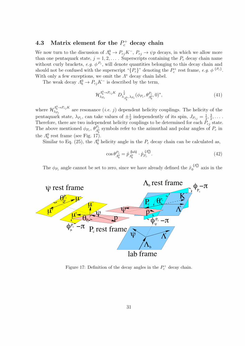
4.3 Matrix element for the P+c decay chain

We now turn to the discussion of Λ0b → PcjK

−, Pcj → ψp decays, in which we allow morethan one pentaquark state, j = 1, 2, . . . . Superscripts containing the Pc decay chain namewithout curly brackets, e.g. φPc , will denote quantities belonging to this decay chain andshould not be confused with the superscript “Pc” denoting the P+

c rest frame, e.g. φ Pc.With only a few exceptions, we omit the Λ∗ decay chain label.

The weak decay Λ0b → PcjK

− is described by the term,

HΛ0b→PcjK

λPcD

12λΛ0b, λPc

(φPc , θPcΛ0b, 0)∗, (41)

where HΛ0b→PcjK

λPcare resonance (i.e. j) dependent helicity couplings. The helicity of the

pentaquark state, λPc , can take values of ±12

independently of its spin, JPcj = 12, 3

2, . . . .

Therefore, there are two independent helicity couplings to be determined for each Pcj state.The above mentioned φPc , θ

PcΛ0b

symbols refer to the azimuthal and polar angles of Pc in

the Λ0b rest frame (see Fig. 17).

Similar to Eq. (25), the Λ0b helicity angle in the Pc decay chain can be calculated as,

cos θPcΛ0b

= plabΛ0b· p Λ

0b

Pc. (42)

The φPc angle cannot be set to zero, since we have already defined the xΛ0b

0 axis in the

K

μ

Λ

−

ΛΛψ *

Λ

−

−*

lab

θΛcPPc

ψ ppψ

b

φ −πφ −π

φ −πcP

b rest frameψ rest frame

Pc rest frame

frame

b

θPc

Pc

PcψP

μμ

+μ

μ+

θψ

c

−

Figure 17: Definition of the decay angles in the P+c decay chain.

31

Λ0b rest frame by the φΛ∗ = 0 convention. According to Eq. (18) (x

Λ0b

0 = xΛ0b

1 ) we have:

~aΛ0b

Λ∗⊥z0 = ~pΛ0b

Λ∗ − (~pΛ0b

Λ∗ · plabΛ0b

) plabΛ0b,

xΛ0b

0 =~aΛ0b

Λ∗⊥z0

|~a Λ0b

Λ∗⊥z0 |. (43)

The φPc angle can be determined in the Λ0b rest frame from

φPc = atan2(

(plabΛ0b× x Λ

0b

0 ) · p Λ0b

Pc, xΛ0b

0 · p Λ0b

Pc

). (44)

The strong decay Pcj → ψp is described by a term

HPcj→ψpλPcψ ,λPcp

DJPcj

λPc , λPcψ −λ

Pcp

(φψ, θPc , 0)∗ RPcj(Mψp), (45)

where φPcψ , θPc are the azimuthal and polar angles of the ψ in the Pc rest frame (see Fig. 17).

They are defined analogously to Eqs. (28)−(30). The zPc

0 direction is defined by the

boost direction from the Λ0b rest frame, which coincides with the −~p PcK direction. This

leads tocos θPc = −p PcK · p Pcψ . (46)

The azimuthal angle of the ψ can now be determined in the Pc rest frame (see Fig. 17)from

φPcψ = atan2(−(p

PcK × x Pc0 ) · p Pcψ , x

Pc0 · p Pcψ

). (47)

In Eq. (45), the xPc

0 direction is defined by the convention that we used in the Λ0b

rest frame. Thus, similar to Eq. (29) we have

~aΛ0b

z0⊥Pc = plabΛ0b− (p

labΛ0b· p Λ

0b

Pc) pΛ0b

Pc,

xPc

0 = −~aΛ0b

z0⊥Pc

|~a Λ0b

z0⊥Pc |. (48)

We have labeled the ψ and p helicities, λPcψ and λPcp , with the Pc superscript to make itclear that the spin quantization axes are different than in the Λ∗ decay chain. Since theψ is an intermediate particle, this has no consequences after we sum (coherently) overλPcψ = −1, 0,+1. The proton, however, is a final-state particle. Before the Pc terms in the

matrix element can be added coherently to the Λ∗ terms, the λPcp states must be rotated toλp states (defined in the Λ∗ decay chain). The proton helicity axes are different, since theproton comes from a decay of different particles in the two decay sequences, the Λ∗ andPc. The quantization axes are along the proton direction in the Λ∗ and the Pc rest frames,thus antiparallel to the particles recoiling against the proton: the K− and ψ, respectively.These directions are preserved when boosting to the proton rest frame (see Fig. 18). Thus,

32

Λ

Λ*K

Λ−

*

zz 00p p PΛ c∗

p

rest framePc

ψ pp

b rest frame

ψP rest framec

ψ K

K Kpp

rest framep

θ

− −

Figure 18: Definition of the θp angle.

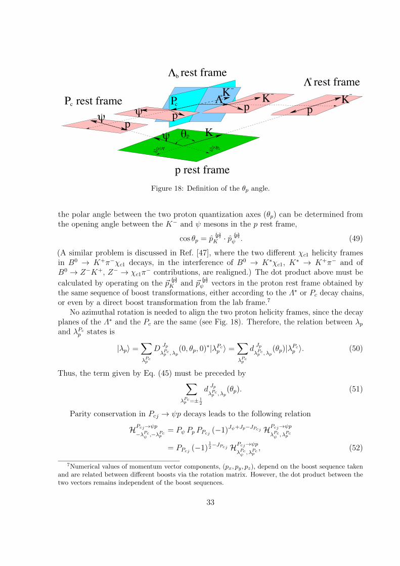
the polar angle between the two proton quantization axes (θp) can be determined fromthe opening angle between the K− and ψ mesons in the p rest frame,

cos θp = ppK · p

pψ . (49)

(A similar problem is discussed in Ref. [47], where the two different χc1 helicity framesin B0 → K+π−χc1 decays, in the interference of B0 → K∗χc1, K

∗ → K+π− and ofB0 → Z−K+, Z− → χc1π

− contributions, are realigned.) The dot product above must be

calculated by operating on the ~ppK and ~p

pψ vectors in the proton rest frame obtained by

the same sequence of boost transformations, either according to the Λ∗ or Pc decay chains,or even by a direct boost transformation from the lab frame.7

No azimuthal rotation is needed to align the two proton helicity frames, since the decayplanes of the Λ∗ and the Pc are the same (see Fig. 18). Therefore, the relation between λpand λPcp states is

|λp〉 =∑λPcp

DJp

λPcp , λp(0, θp, 0)∗|λPcp 〉 =

∑λPcp

dJp

λPcp , λp(θp)|λPcp 〉. (50)

Thus, the term given by Eq. (45) must be preceded by∑λPcp =± 1

2

dJp

λPcp , λp(θp). (51)

Parity conservation in Pcj → ψp decays leads to the following relation

HPcj→ψp−λPcψ ,−λPcp

= Pψ Pp PPcj (−1)Jψ+Jp−JPcj HPcj→ψpλPcψ , λPcp

= PPcj (−1)12−JPcj HPcj→ψp

λPcψ , λPcp, (52)

7Numerical values of momentum vector components, (px, py, pz), depend on the boost sequence takenand are related between different boosts via the rotation matrix. However, the dot product between thetwo vectors remains independent of the boost sequences.

33

where PPcj is the parity of the Pcj state. This relation reduces the number of inde-pendent helicity couplings to be determined from the data to 2 for JPcj = 1

2and 3 for

JPcj ≥ 32. Since the helicity couplings enter the matrix element formula as a product,

HΛ0b→PcjK

λPcHPcj→ψpλPcψ , λPcp

, the relative magnitude and phase of these two sets must be fixed by a

convention. For example, HΛ0b→PcjK

λPc=− 12

can be set to (1, 0) for every Pcj resonance, in which

case HΛ0b→PcjK

λPc=+ 12

develops a meaning of the complex ratio of HΛ0b→PcjK

λPc=+ 12

/HΛ0b→PcjK

λPc=− 12

, while all

HPcj→ψpλPcψ , λPcp

couplings should have both real and imaginary parts free in the fit.

The term RPcj (Mψp) describes the ψp invariant mass distribution of the Pcj resonanceand is given by Eq. (31) after appropriate substitutions. Angular momentum conservation

limits LPcjΛ0b

in Λ0b → PcjK

− decays to JPcj ± 12. The angular momentum conservation also

imposes max(JPcj − 32, 0) ≤ LPcj ≤ JPcj + 3

2, which is further restricted by the parity

conservation in the Pcj decays, PPcj = (−1)LPcj+1. We assume the minimal values of LPcjΛ0b

and of LPcj in RPcj(mψp).The electromagnetic decay ψ → µ+µ− in the Pc decay chain contributes a term

D 1λPcψ ,∆λPcµ

(φPcµ , θPcψ , 0)∗, (53)

which is the same as Eq. (35), except that since the ψ meson comes from the decay ofdifferent particles in the two decay chains, the azimuthal and polar angle of the muon inthe ψ rest frame, φPcµ , θPcψ , are different from φµ, θψ introduced in the Λ∗ decay chain. Theψ helicity axis is along the boost direction from the Pc to the ψ rest frames, which is givenby

zψ

0Pc = − p ψp , (54)

and socos θPcψ = −p ψp · p ψµ . (55)

The x axis is inherited from the Pc rest frame (Eq. (19)),

~aPcz0⊥ψ = −~p PcK + (~p

PcK · p Pcψ ) p

Pcψ

xψ

0Pc = x

Pc3 = −

~aPcz0⊥ψ

|~a Pcz0⊥ψ |, (56)

which leads to

φPcµ = atan2(−(p ψp × x ψ0

Pc) · p ψµ , xψ

0Pc · p ψµ

). (57)

Since the muons are final-state particles, their helicity states in the Pc decay chain,|λPcµ 〉, need to be rotated to the muon helicity states in the Λ∗ decay chain, |λµ〉, beforethe Pc matrix element terms can be coherently added to the Λ∗ matrix element terms.The situation is simpler than for the rotation of the proton helicities discussed above, as

34

the muons come from the ψ decay in both decay chains. This makes the polar angle θµ

(analogous to θp in Eq. (51)) equal to zero, which leads to d12

λPcµ , λµ(0) = δλPcµ , λµ

, where δi,j

is the Kronecker symbol. However, the muon helicity states are not identical since the xaxes are offset by the azimuthal angle αµ. Since the boost to the µ rest frame is the samefor both decay chains (i.e. always from the ψ rest frame), we can determine αµ in the ψrest frame

αµ = atan2(

(zψ

3 × x ψ3Pc) · x ψ3

Λ∗ , xψ

3Pc · x ψ3

Λ∗), (58)

where zψ

3 = pψµ , and from Eq. (19)

xψ

3Pc = − a ψz0⊥µ

Pc , (59)

~aψz0⊥µ

Pc = − p ψp + (p ψp · p ψµ ) p ψµ , (60)

as well as

xψ

3Λ∗ = − a ψz0⊥µ

Λ∗ , (61)

~aψz0⊥µ

Λ∗ = − p ψΛ∗ + (pψΛ∗ · p

ψµ ) p ψµ . (62)

The term aligning the muon helicity states between the two reference frames is given by∑λPcµ

DJµ

λPcµ λµ(αµ, 0, 0)∗ =

∑λPcµ

ei λPcµ αµδλPcµ , λµ

= ei λµαµ . (63)

The transformation of µ− states will be similar to that of the µ+ states, except that sincezψ will have the opposite direction, αµ+ = −αµ− . The transformation of |λPcµ+〉|λPcµ−〉 to|λµ+〉|λµ−〉 states will require multiplying the terms for the Pc decay chain by

ei λµαµei λµαµ = ei (λµ−λµ)αµ = ei∆λµαµ . (64)

An alternative derivation of Eq. (64) is discussed in Ref. [8] (Eqs. (20)−(22) therein) forthe interference of B0 → K∗ψ, K∗ → Kπ and of B0 → ZK−, Z → ψπ (ψ → `+`−) terms,which are analogous to the two decay chains discussed here with the substitution B0 → Λ0

b ,K∗ → Λ∗, Z → Pc and π → p. The rotation by αµ about the `+ direction in the ψ restframe in the Z decay chain is incorporated by setting γ = αµ, instead of γ = 0 in Eq. (53).This leads to the same formulae since

D 1λPcψ ,∆λµ

(φPcµ , θPcψ , αµ)∗ = D 1

λPcψ ,∆λµ(φPcµ , θ

Pcψ , 0)∗ ei∆λµαµ . (65)

We use the more generic derivation here to demonstrate that the methods of transformingthe muon and proton helicity states between the two decay chains are the same.

Collecting terms from the three subsequent decays in the Pc chain together,

M PcλΛ0b, λPcp ,∆λPcµ

=ei λΛ0bφPc∑j

RPcj(Mψp)∑λPcψ

ei λPcψ φPcµ d 1

λPcψ ,∆λµ(θPcψ )

×∑λPc

HΛ0b→PcjK

λPcei λPcφ

Pcψ d

12λΛ0b, λPc

(θPcΛ0b)HPcj→ψp

λPcψ , λPcpdJPcj

λPc , λPcψ −λ

Pcp

(θPc), (66)

35

and adding them coherently to the Λ∗ matrix element, via appropriate relation of|λp〉|λµ+〉|λµ−〉 to |λPcp 〉|λPcµ+〉|λPcµ−〉 states as discussed above, leads to the final matrixelement squared

|M|2 =∑

λΛ0b=± 1

2

∑λp=± 1

2

∑∆λµ=±1

∣∣∣∣∣∣MΛ∗

λΛ0b, λp,∆λµ + ei∆λµαµ

∑λPcp

d12

λPcp , λp(θp)MPc

λΛ0b, λPcp ,∆λµ

∣∣∣∣∣∣2

,

(67)where we set PΛ0

b = 0. As a cross-check, fitting the Λ0b polarization to the data with

the default Λ∗ and P+c model yields a value consistent with zero, PΛ0

b = (−2.0 ± 2.3)%(statistical error only).

Assuming approximate CP symmetry, the helicity couplings for Λ0b and Λ0

b can be madeequal, but the calculation of the angles requires some care, since parity (P ) conservationdoes not change polar (i.e. helicity) angles, but does change azimuthal angles. Thus, notonly must ~pµ+ be used instead of ~pµ− for Λ0

b candidates (with K+ and p in the final-state)in Eqs. (36), (37), (55), (57) and (58), but also all azimuthal angles must be reflected beforeentering the matrix element formula: φK → −φK , φµ → −φµ, φPc → −φPc , φPcψ → −φ

Pcψ ,

φPcµ → −φPcµ and αµ → −αµ [8].It is clear from Eq. (67) that various Λ∗n and Pc resonances interfere in the differential

distributions. By integrating the matrix element squared over the entire phase space theinterferences cancel in the integrated rates unless the resonances belong to the same decaychain and have the same quantum numbers.8

4.4 Reduction of the number of helicity couplings

A possible reduction of the helicity couplings can be achieved by relating them to the LScouplings (BL,S) using Clebsch-Gordan coefficients

HA→BCλB ,λC

=∑L

∑S

√2L+1

2JA+1BL,S

(JB JC SλB −λC λB − λC

)×(L S JA0 λB − λC λB − λC

),

(68)and then restricting the L values. Here L is the orbital angular momentum in the decay,and S is the total spin of the daughters, ~S = ~JB + ~JC (|JB − JC | ≤ S ≤ JB + JC). If theenergy release in the decay, Q = MA−MB −MC , is small, Q/MA 1, then higher valuesof L should be suppressed; this effect is usually called “the angular momentum barrier.”Applying this approach to Λ0

b → ψΛ∗n decays, the lowest LΛ∗nΛ0b

value (Lmin) corresponds to a

single possible value of S, thus reducing the number of couplings to fit, from 4 (JΛ∗n = 12)

or 6 (JΛ∗n ≥32), to just one BL,S coupling per resonance. Accepting also Lmin + 1 values,

gives three BL,S couplings to fit per resonance.

In Λ0b → PcjK

− decays, S = JPcj and LPcjΛ0b

= JPcj ± 12. Taking only the lower L

PcjΛ0b

value reduces the number of couplings from 2 to 1. Since its magnitude and phase

8For Λ∗n−Pc, the λΛ0b

= +1/2 interference terms have the opposite effect to the λΛ0b

= −1/2 interferenceterms.

36

convention can be absorbed into HPcj→ψpλPcψ , λPcp

(see the discussion in Sec. 4.3), one can simply

set BΛ0b→PcjK

JPcj−12,JPcj

= (1, 0) in this approach.

The reduction of couplings to fit for Pcj → ψp decays depends on the spin and parityof the Pcj state. S can take values of 1

2and 3

2. Values of LPcj must be odd (even) for even

(odd) PPcj . For a JPPcj = 12

+state, only LPcj = 1 is allowed with the two possible values of

S. Therefore, no reduction of couplings is possible. For a JPPcj = 12

−state, LPcj = 0, 2 are

allowed, each corresponding to one S value. Therefore, the number of couplings to fit canbe reduced from 2 to 1 when taking LPcj = 0. Gains can be larger for JPcj ≥ 3

2states.

Even if no reduction in parameters is achieved, expressing the helicity couplings viacorresponding BL,S couplings using Eq. (68) is useful, since it automatically implements theparity constraints (Eq. (52)) by restricting possible L values. Since the overall magnitudeof the matrix element does not affect the normalized signal PDF, and because its overallphase also drops out when taking its modulus, we fix the magnitude and phase convention

by setting BΛ0b→Λ(1520)J/ψ

0, 12

= (1, 0).

5 Details of fitting techniques

The matrix element given by Eq. (67), is a 6-dimensional (6D) function of mKp andΩ and depends on the fit parameters, −→ω , which represent independent helicity or LScouplings, and possibly masses and widths of resonances, M(mKp, Ω|−→ω ). We performan unbinned maximum likelihood fit of these parameters to the 6D data by minimizing−2 lnL(−→ω ) = −2 ln

∑iP(mKp i, Ωi|−→ω ) with respect to −→ω . The signal PDF is obtained

by multiplying the matrix element squared with the selection efficiency, ε(mKp, Ω),

Psig(mKp, Ω|−→ω ) =1

I(−→ω )|M(mKp, Ω|−→ω )|2 Φ(mKp)ε(mKp, Ω), (69)

where Φ(mKp) is the phase space function equal to p q, where p is the momentum of theKp system (i.e. Λ∗) in the Λ0

b rest frame, and q is the momentum of K− in the Λ∗ restframe, and I(−→ω ) is the normalization integral.

We use two fit algorithms that were independently coded and that differ in the approachused for background subtraction. The sFit procedure uses the sPlot technique described inRef. [31] to subtract background from the log-likelihood sum. It has been used in previousLHCb analyses, e.g. measurement of φs in B0

s → J/ψφ decays [48]. The data in the entire5480− 5760 MeV range are passed to the fitter. Candidates are assigned “sWeights” (Wi)according to their mJ/ψpK value with the signal and background probabilities determinedby the fit to the mJ/ψpK distribution,

− 2 lnL(−→ω ) = −2sW∑i

Wi lnP(mKp i, Ωi|−→ω ), (70)

where sW ≡∑

iWi/∑

iWi2 is a constant factor accounting for the effect of the background

subtraction on the statistical uncertainty. Candidates in the sideband region have negative

37

sWeights which on average compensate for the background events present in the peakregion, where events have positive sWeights. From signal simulations, we see significantvariations of Λ0

b → J/ψpK− invariant mass resolution as functions of cos θΛ0b

and cos θJ/ψ .The background distributions also vary in intensity and shape with these two variables. Nostrong variation is seen for the other fitting observables. To determine the sWeights, theevents are divided into 4 | cos θJ/ψ | × 8 cos θΛ0

bbins. A separate fit to the Λ0

b → J/ψpK−

invariant mass distribution of each bin is performed.In the sFit approach the total PDF is equal to the signal PDF, as the background is

subtracted from the log-likelihood sum using sWeights,

−2 lnL(−→ω ) =− 2sW∑i

Wi lnPsig(mKp i, Ωi|−→ω )

=− 2sW∑i

Wi ln |M(mKp i, Ωi|−→ω )|2 + 2sW ln I(−→ω )∑i

Wi

− 2sW∑i

Wi ln[Φ(mKp i)ε(mKp i, Ωi)]. (71)

The last term does not depend on the fitted parameters −→ω and is therefore dropped. Theefficiency still appears in the normalization integral. The integration is done without theneed to parameterize the efficiency, by summing the matrix element squared over thesimulated events that are generated uniformly in phase space and passed through thedetector modeling and the data selection procedure,

I(−→ω ) ≡∫|M(mKp, Ω|−→ω )|2 Φ(mKp)ε(mKp, Ω) dmKp dΩ

∝NMC∑j

wMCj |M(mKp j, Ωj|−→ω )|2 , (72)

where wMCj are the weights given to the simulated events to improve the agreement between

data and simulations. They include particle identification weights obtained from calibrationsamples of Λ→ pπ− and D0 → K−π+ as functions of momentum and pseudorapidity ofthe protons and kaons. They also include a weight correcting the overall efficiency for thedependence on the charged track multiplicity of events, determined from the ratio of thebackground-subtracted data and the signal simulations. Imperfect description of the Λ0

b

production kinematics in our simulation is corrected in a similar way via a weight thatdepends on the p and pT of the Λ0

b baryon. The final weights are the ratio of the data andthe simulations as a function of proton and kaon momenta.

In the cFit approach, candidates are not weighted (Wi = 1). The data that are fittedare restricted to be within a ±2σ mass window around the Λ0

b mass peak, in the interval5605.7 < mJ/ψpK < 5635.8 MeV. The background is represented explicitly in the fittedPDF, with the integrated background probability set to β = 5.4% as determined from thefit to the J/ψK−p mass distribution,

P(mKp, Ω|−→ω ) = (1− β)Psig(mKp, Ω|−→ω ) + β Pbkg(mKp, Ω). (73)

38

The 6-dimensional background parameterization Pbkg(mKp, Ω) is developed using thebackground sample in which the Λ0

b candidate invariant mass is more than 5σ away fromthe peak, specifically within the intervals 5480.0− 5583.2 MeV and 5658.3− 5760.0 MeV.We minimize the negative log-likelihood defined as,

− 2 lnL(−→ω ) =

− 2∑i

ln

[(1− β)

|M(mKp i, Ωi|−→ω )|2 Φ(mKp i)ε(mKp i, Ωi)

I(−→ω )+ βPubkg(mKp i, Ωi)

Ibkg

]

= −2∑i

ln

[|M(mKp i, Ωi|−→ω )|2 +

β I(−→ω )

(1− β)Ibkg

Pubkg(mKp i, Ωi)

Φ(mKp i)ε(mKp i, Ωi)

]+ 2N ln I(−→ω ) + constant, (74)

where N is the number of candidates, and Pubkg(mKp, Ω) is the unnormalized backgrounddensity proportional to the density of sideband candidates, with its normalization deter-mined by9

Ibkg ≡∫Pubkg(mKp) dmKp dΩ ∝

∑j

wMCj

Pubkg(mKp j, Ωj)

Φ(mKp j)ε(mKp j, Ωj). (75)

The background term is then efficiency-corrected so it can be added to the efficiency-independent signal probability expressed by |M|2. This way the efficiency parametrization,ε(mKp, Ω), influences only the background component which affects only a tiny part ofthe total PDF, while the efficiency corrections to the signal part enter Eq. (72).

The efficiency in the background term is assumed to factorize as

ε(mKp, Ω) = ε1(mKp, cos θ∗Λ)ε2(cos θΛ0b|mKp)ε3(cos θJ/ψ |mKp)ε4(φK |mKp)ε5(φµ|mKp).

(76)The ε1(mKp, cos θ∗Λ) term is obtained from a 2D histogram of the simulated events weightedby 1/(p q). A bi-cubic interpolation is used to interpolate between bin centers. The otherterms are again built from 2D histograms, but with each bin divided by the number ofsimulated events in the corresponding mKp slice to remove the leading dependence on thismass, which is already taken into account in the first term. The leading variation of theefficiency is in the ε1(mKp, cos θ∗Λ) term which is visualized in the normal Dalitz variables(m2

J/ψp,m2Kp) in Fig. 19(a) instead of the “rectangular Dalitz plane” variables (mKp, cos θ∗Λ)

used to parameterize this variation.The background PDF, Pubkg(mKp, Ω)/Φ(mKp), is built using the same approach,

Pubkg(mKp, Ω)

Φ(mKp)= Pbkg1(mKp, cos θ∗Λ)Pbkg2(cos θΛ0

b|mKp)

× Pbkg3(cos θJ/ψ |mKp)Pbkg4(φK |mKp)Pbkg5(φµ|mKp). (77)

A visualization of Pbkg1(mKp, cos θ∗Λ) on the Dalitz plane is shown in Fig. 19(b).

9Note that the distribution of MC events includes both the Φ(mKp) and ε(mKp, Ω) factors, whichcancel their product in the numerator.

39

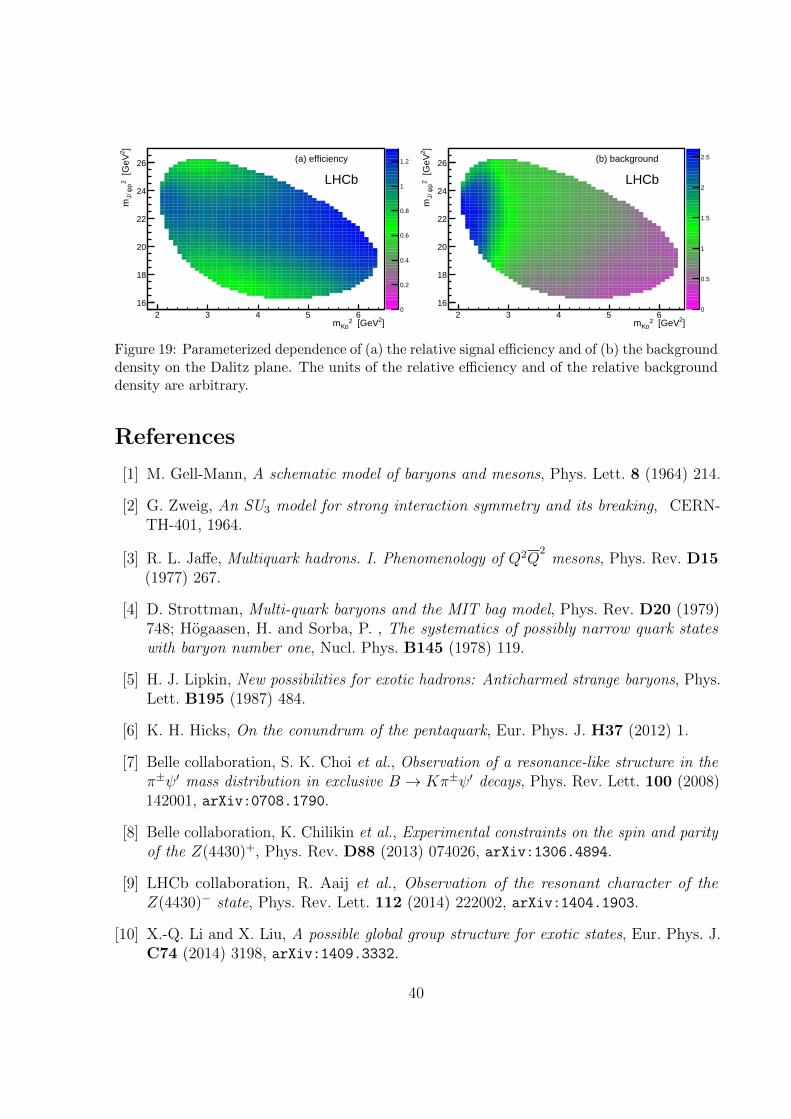
]2 [GeV2Kpm

2 3 4 5 6

]2 [

GeV

2p

ψJ/

m

16

18

20

22

24

26

0

0.2

0.4

0.6

0.8

1

1.2

LHCb

(a) efficiency

]2 [GeV2Kpm

2 3 4 5 6

]2 [

GeV

2p

ψJ/

m

16

18

20

22

24

26

0

0.5

1

1.5

2

2.5

LHCb

(b) background

Figure 19: Parameterized dependence of (a) the relative signal efficiency and of (b) the backgrounddensity on the Dalitz plane. The units of the relative efficiency and of the relative backgrounddensity are arbitrary.

References

[1] M. Gell-Mann, A schematic model of baryons and mesons, Phys. Lett. 8 (1964) 214.

[2] G. Zweig, An SU3 model for strong interaction symmetry and its breaking, CERN-TH-401, 1964.

[3] R. L. Jaffe, Multiquark hadrons. I. Phenomenology of Q2Q2

mesons, Phys. Rev. D15(1977) 267.

[4] D. Strottman, Multi-quark baryons and the MIT bag model, Phys. Rev. D20 (1979)748; Hogaasen, H. and Sorba, P. , The systematics of possibly narrow quark stateswith baryon number one, Nucl. Phys. B145 (1978) 119.

[5] H. J. Lipkin, New possibilities for exotic hadrons: Anticharmed strange baryons, Phys.Lett. B195 (1987) 484.

[6] K. H. Hicks, On the conundrum of the pentaquark, Eur. Phys. J. H37 (2012) 1.

[7] Belle collaboration, S. K. Choi et al., Observation of a resonance-like structure in theπ±ψ′ mass distribution in exclusive B → Kπ±ψ′ decays, Phys. Rev. Lett. 100 (2008)142001, arXiv:0708.1790.

[8] Belle collaboration, K. Chilikin et al., Experimental constraints on the spin and parityof the Z(4430)+, Phys. Rev. D88 (2013) 074026, arXiv:1306.4894.

[9] LHCb collaboration, R. Aaij et al., Observation of the resonant character of theZ(4430)− state, Phys. Rev. Lett. 112 (2014) 222002, arXiv:1404.1903.

[10] X.-Q. Li and X. Liu, A possible global group structure for exotic states, Eur. Phys. J.C74 (2014) 3198, arXiv:1409.3332.

40

[11] LHCb collaboration, R. Aaij et al., Precision measurement of the ratio of the Λ0b to

B0

lifetimes, Phys. Lett. B734 (2014) 122, arXiv:1402.6242; LHCb collaboration,R. Aaij et al., Precision measurement of the Λ0

b baryon lifetime, Phys. Rev. Lett. 111(2013) 102003, arXiv:1307.2476.

[12] Particle Data Group, K. A. Olive et al., Review of particle physics, Chin. Phys. C38(2014) 090001.

[13] LHCb collaboration, A. A. Alves Jr. et al., The LHCb detector at the LHC, JINST 3(2008) S08005.

[14] R. Aaij et al., Performance of the LHCb Vertex Locator, JINST 9 (2014) P09007,arXiv:1405.7808.

[15] R. Arink et al., Performance of the LHCb Outer Tracker, JINST 9 (2014) P01002,arXiv:1311.3893.

[16] M. Adinolfi et al., Performance of the LHCb RICH detector at the LHC, Eur. Phys.J. C73 (2013) 2431, arXiv:1211.6759.

[17] A. A. Alves Jr. et al., Performance of the LHCb muon system, JINST 8 (2013) P02022,arXiv:1211.1346.

[18] LHCb collaboration, R. Aaij et al., First observation of B0s → J/ψf0(980) decays,

Phys. Lett. B698 (2011) 115, arXiv:1102.0206.

[19] L. Breiman, J. H. Friedman, R. A. Olshen, and C. J. Stone, Classification and regres-sion trees, Wadsworth international group, Belmont, California, USA, 1984; A. Hoeckeret al., TMVA – Toolkit for multivariate data analysis, arXiv:physics/0703039.

[20] T. Sjostrand, S. Mrenna, and P. Skands, PYTHIA 6.4 physics and manual, JHEP05 (2006) 026, arXiv:hep-ph/0603175; T. Sjostrand, S. Mrenna, and P. Skands,A brief introduction to PYTHIA 8.1, Comput. Phys. Commun. 178 (2008) 852,arXiv:0710.3820.

[21] I. Belyaev et al., Handling of the generation of primary events in Gauss, the LHCbsimulation framework, J. Phys. Conf. Ser. 331 (2011) 032047.

[22] Geant4 collaboration, S. Agostinelli et al., Geant4: A simulation toolkit, Nucl. Instrum.Meth. A506 (2003) 250; Geant4 collaboration, J. Allison et al., Geant4 developmentsand applications, IEEE Trans. Nucl. Sci. 53 (2006) 270.

[23] M. Clemencic et al., The LHCb simulation application, Gauss: Design, evolution andexperience, Journal of Physics: Conference Series 331 (2011) 032023.

[24] D. Martınez Santos and F. Dupertuis, Mass distributions marginalized over per-eventerrors, Nucl. Instrum. Meth. A764 (2014) 150, arXiv:1312.5000.

41

[25] W. D. Hulsbergen, Decay chain fitting with a Kalman filter, Nucl. Instrum. Meth.A552 (2005) 566, arXiv:physics/0503191.

[26] R. H. Dalitz, On the analysis of τ -meson data and the nature of the τ -meson, Phil.Mag. 44 (1953) 1068.

[27] S. U. Chung, Spin formalisms, CERN-71-08; J. D. Richman, An experimenter’sguide to the helicity formalism, CALT-68-1148; M. Jacob and G. C. Wick, On thegeneral theory of collisions for particles with spin, Annals Phys. 7 (1959) 404.

[28] F. Von Hippel and C. Quigg, Centrifugal-barrier effects in resonance partial decaywidths, shapes, and production amplitudes, Phys. Rev. D5 (1972) 624.

[29] S. M. Flatte, Coupled-channel analysis of the πη and KK systems near KK threshold,Phys. Lett. B63 (1976) 224.

[30] Soffer, Jacques and Tornqvist, Nils A. , Origin of the polarization for inclusive Λproduction in pp collisions, Phys. Rev. Lett. 68 (1992) 907.

[31] M. Pivk and F. R. Le Diberder, sPlot: A statistical tool to unfold data distributions,Nucl. Instrum. Meth. A555 (2005) 356, arXiv:physics/0402083; Y. Xie, sFit: amethod for background subtraction in maximum likelihood fit, arXiv:0905.0724.

[32] F. James, Statistical methods in experimental physics, World Scientific Publishing,2006.

[33] J. F. Donoghue, E. Golowich, W. A. Ponce, and B. R. Holstein, Analysis of ∆S=1nonleptonic weak decays and the ∆I=1/2 rule, Phys. Rev. D21 (1980) 186.

[34] LHCb collaboration, R. Aaij et al., Observation of overlapping spin-1 and spin-3 D0K− resonances at mass 2.86 GeV/c2, Phys. Rev. Lett. 113 (2014) 162001,arXiv:1407.7574; LHCb collaboration, R. Aaij et al., Dalitz plot analysis of B0

s →D0K−π+ decays, Phys. Rev. D90 (2014) 072003, arXiv:1407.7712.

[35] G. C. Rossi and G. Veneziano, A possible description of baryon dynamics in dual andgauge theories, Nucl. Phys. B123 (1977) 507.

[36] L. Maiani, F. Piccinini, A. D. Polosa, and V. Riquer, Diquark-antidiquarks withhidden or open charm and the nature of X(3872), Phys. Rev. D71 (2005) 014028,arXiv:hep-ph/0412098.

[37] R. L. Jaffe and F. Wilczek, Diquarks and exotic spectroscopy, Phys. Rev. Lett. 91(2003) 232003, arXiv:hep-ph/0307341.

[38] A. Chandra, A. Bhattacharya, and B. Chakrabarti, Heavy pentaquarks and doublyheavy baryons in quasiparticle approach, Mod. Phys. Lett. A27 (2012) 1250006.

42

[39] M. Karliner and H. J. Lipkin, A diquark - triquark model for the KN pentaquark,Phys. Lett. B575 (2003) 249, arXiv:hep-ph/0402260.

[40] J.-J. Wu, R. Molina, E. Oset, and B. S. Zou, Prediction of narrow N∗ and Λ∗

resonances with hidden charm above 4 GeV, Phys. Rev. Lett. 105 (2010) 232001,arXiv:1007.0573.

[41] M. B. Voloshin and L. B. Okun, Hadron molecules and charmonium atom, JETP Lett.23 (1976) 333; A. De Rujula, H. Georgi, and S. L. Glashow, Molecular charmonium:a new spectroscopy?, Phys. Rev. Lett. 38 (1977) 317; N. A. Tornqvist, Possible largedeuteron–like meson meson states bound by pions, Phys. Rev. Lett. 67 (1991) 556;N. A. Tornqvist, From the deuteron to deusons, an analysis of deuteron–like mesonmeson bound states, Z. Phys. C61 (1994) 525, arXiv:hep-ph/9310247; Z.-C. Yanget al., The possible hidden-charm molecular baryons composed of anti-charmed mesonand charmed baryon, Chin. Phys. C36 (2012) 6, arXiv:1105.2901; W. L. Wang,F. Huang, Z. Y. Zhang, and B. S. Zou, ΣcD and ΛcD states in a chiral quark model,Phys. Rev. C84 (2011) 015203, arXiv:1101.0453; M. Karliner and J. L. Rosner,New exotic meson and baryon resonances from doubly-heavy hadronic molecules,arXiv:1506.06386.

[42] E. S. Swanson, Cusps and exotic charmonia, arXiv:1504.07952.

[43] E. S. Swanson, Zb and Zc exotic states as coupled channel cusps, Phys. Rev. D91(2015) 034009, arXiv:1409.3291.

[44] D. V. Bugg, An explanation of Belle states Zb(10610) and Zb(10650), Europhys. Lett.96 (2011) 11002, arXiv:1105.5492.

[45] J. M. Blatt and V. F. Weisskopf, Theoretical Nuclear Physics, Springer-Verlag, 1979.

[46] LHCb collaboration, R. Aaij et al., Measurements of the Λ0b → J/ψΛ decay amplitudes

and the Λ0b polarization in pp collisions at

√s = 7 TeV, Phys. Lett. B724 (2013) 27,

arXiv:1302.5578.

[47] Belle collaboration, R. Mizuk et al., Observation of two resonance-like structures inthe π+χc1 mass distribution in exclusive B0 → K−π+χc1 decays, Phys. Rev. D78(2008) 072004, arXiv:0806.4098.

[48] LHCb, R. Aaij et al., Precision measurement of CP violation in B0s → J/ψK+K−

decays, Phys. Rev. Lett. 114 (2015) 041801, arXiv:1411.3104.

43

LHCb collaboration

R. Aaij38, B. Adeva37, M. Adinolfi46, A. Affolder52, Z. Ajaltouni5, S. Akar6, J. Albrecht9,F. Alessio38, M. Alexander51, S. Ali41, G. Alkhazov30, P. Alvarez Cartelle53, A.A. Alves Jr57,S. Amato2, S. Amerio22, Y. Amhis7, L. An3, L. Anderlini17, J. Anderson40, G. Andreassi39,M. Andreotti16,f , J.E. Andrews58, R.B. Appleby54, O. Aquines Gutierrez10, F. Archilli38,P. d’Argent11, A. Artamonov35, M. Artuso59, E. Aslanides6, G. Auriemma25,m, M. Baalouch5,S. Bachmann11, J.J. Back48, A. Badalov36, C. Baesso60, W. Baldini16,38, R.J. Barlow54,C. Barschel38, S. Barsuk7, W. Barter38, V. Batozskaya28, V. Battista39, A. Bay39, L. Beaucourt4,J. Beddow51, F. Bedeschi23, I. Bediaga1, L.J. Bel41, V. Bellee39, N. Belloli20, I. Belyaev31,E. Ben-Haim8, G. Bencivenni18, S. Benson38, J. Benton46, A. Berezhnoy32, R. Bernet40,A. Bertolin22, M.-O. Bettler38, M. van Beuzekom41, A. Bien11, S. Bifani45, P. Billoir8, T. Bird54,A. Birnkraut9, A. Bizzeti17,h, T. Blake48, F. Blanc39, J. Blouw10, S. Blusk59, V. Bocci25,A. Bondar34, N. Bondar30,38, W. Bonivento15, S. Borghi54, M. Borsato7, T.J.V. Bowcock52,E. Bowen40, C. Bozzi16, S. Braun11, M. Britsch10, T. Britton59, J. Brodzicka54, N.H. Brook46,A. Bursche40, J. Buytaert38, S. Cadeddu15, R. Calabrese16,f , M. Calvi20,j , M. Calvo Gomez36,o,P. Campana18, D. Campora Perez38, L. Capriotti54, A. Carbone14,d, G. Carboni24,k,R. Cardinale19,i, A. Cardini15, P. Carniti20, L. Carson50, K. Carvalho Akiba2,38, G. Casse52,L. Cassina20,j , L. Castillo Garcia38, M. Cattaneo38, Ch. Cauet9, G. Cavallero19, R. Cenci23,s,M. Charles8, Ph. Charpentier38, M. Chefdeville4, S. Chen54, S.-F. Cheung55, N. Chiapolini40,M. Chrzaszcz40, X. Cid Vidal38, G. Ciezarek41, P.E.L. Clarke50, M. Clemencic38, H.V. Cliff47,J. Closier38, V. Coco38, J. Cogan6, E. Cogneras5, V. Cogoni15,e, L. Cojocariu29, G. Collazuol22,P. Collins38, A. Comerma-Montells11, A. Contu15,38, A. Cook46, M. Coombes46, S. Coquereau8,G. Corti38, M. Corvo16,f , B. Couturier38, G.A. Cowan50, D.C. Craik48, A. Crocombe48,M. Cruz Torres60, S. Cunliffe53, R. Currie53, C. D’Ambrosio38, E. Dall’Occo41, J. Dalseno46,P.N.Y. David41, A. Davis57, K. De Bruyn41, S. De Capua54, M. De Cian11, J.M. De Miranda1,L. De Paula2, P. De Simone18, C.-T. Dean51, D. Decamp4, M. Deckenhoff9, L. Del Buono8,N. Deleage4, M. Demmer9, D. Derkach55, O. Deschamps5, F. Dettori38, B. Dey21, A. Di Canto38,F. Di Ruscio24, H. Dijkstra38, S. Donleavy52, F. Dordei11, M. Dorigo39, A. Dosil Suarez37,D. Dossett48, A. Dovbnya43, K. Dreimanis52, L. Dufour41, G. Dujany54, F. Dupertuis39,P. Durante38, R. Dzhelyadin35, A. Dziurda26, A. Dzyuba30, S. Easo49,38, U. Egede53,V. Egorychev31, S. Eidelman34, S. Eisenhardt50, U. Eitschberger9, R. Ekelhof9, L. Eklund51,I. El Rifai5, Ch. Elsasser40, S. Ely59, S. Esen11, H.M. Evans47, T. Evans55, A. Falabella14,C. Farber38, N. Farley45, S. Farry52, R. Fay52, D. Ferguson50, V. Fernandez Albor37,F. Ferrari14, F. Ferreira Rodrigues1, M. Ferro-Luzzi38, S. Filippov33, M. Fiore16,38,f ,M. Fiorini16,f , M. Firlej27, C. Fitzpatrick39, T. Fiutowski27, K. Fohl38, P. Fol53, M. Fontana15,F. Fontanelli19,i, R. Forty38, O. Francisco2, M. Frank38, C. Frei38, M. Frosini17, J. Fu21,E. Furfaro24,k, A. Gallas Torreira37, D. Galli14,d, S. Gallorini22,38, S. Gambetta50,M. Gandelman2, P. Gandini55, Y. Gao3, J. Garcıa Pardinas37, J. Garra Tico47, L. Garrido36,D. Gascon36, C. Gaspar38, R. Gauld55, L. Gavardi9, G. Gazzoni5, A. Geraci21,u, D. Gerick11,E. Gersabeck11, M. Gersabeck54, T. Gershon48, Ph. Ghez4, A. Gianelle22, S. Gianı39,V. Gibson47, O. G. Girard39, L. Giubega29, V.V. Gligorov38, C. Gobel60, D. Golubkov31,A. Golutvin53,31,38, A. Gomes1,a, C. Gotti20,j , M. Grabalosa Gandara5, R. Graciani Diaz36,L.A. Granado Cardoso38, E. Grauges36, E. Graverini40, G. Graziani17, A. Grecu29,E. Greening55, S. Gregson47, P. Griffith45, L. Grillo11, O. Grunberg63, B. Gui59, E. Gushchin33,Yu. Guz35,38, T. Gys38, T. Hadavizadeh55, C. Hadjivasiliou59, G. Haefeli39, C. Haen38,

44

S.C. Haines47, S. Hall53, B. Hamilton58, X. Han11, S. Hansmann-Menzemer11, N. Harnew55,S.T. Harnew46, J. Harrison54, J. He38, T. Head39, V. Heijne41, K. Hennessy52, P. Henrard5,L. Henry8, J.A. Hernando Morata37, E. van Herwijnen38, M. Heß63, A. Hicheur2, D. Hill55,M. Hoballah5, C. Hombach54, W. Hulsbergen41, T. Humair53, N. Hussain55, D. Hutchcroft52,D. Hynds51, M. Idzik27, P. Ilten56, R. Jacobsson38, A. Jaeger11, J. Jalocha55, E. Jans41,A. Jawahery58, F. Jing3, M. John55, D. Johnson38, C.R. Jones47, C. Joram38, B. Jost38,N. Jurik59, S. Kandybei43, W. Kanso6, M. Karacson38, T.M. Karbach38,†, S. Karodia51,M. Kecke11, M. Kelsey59, I.R. Kenyon45, M. Kenzie38, T. Ketel42, B. Khanji20,38,j ,C. Khurewathanakul39, S. Klaver54, K. Klimaszewski28, O. Kochebina7, M. Kolpin11,I. Komarov39, R.F. Koopman42, P. Koppenburg41,38, M. Kozeiha5, L. Kravchuk33, K. Kreplin11,M. Kreps48, G. Krocker11, P. Krokovny34, F. Kruse9, W. Krzemien28, W. Kucewicz26,n,M. Kucharczyk26, V. Kudryavtsev34, A. K. Kuonen39, K. Kurek28, T. Kvaratskheliya31,D. Lacarrere38, G. Lafferty54, A. Lai15, D. Lambert50, G. Lanfranchi18, C. Langenbruch48,B. Langhans38, T. Latham48, C. Lazzeroni45, R. Le Gac6, J. van Leerdam41, J.-P. Lees4,R. Lefevre5, A. Leflat32,38, J. Lefrancois7, O. Leroy6, T. Lesiak26, B. Leverington11, Y. Li7,T. Likhomanenko65,64, M. Liles52, R. Lindner38, C. Linn38, F. Lionetto40, B. Liu15, X. Liu3,D. Loh48, I. Longstaff51, J.H. Lopes2, D. Lucchesi22,q, M. Lucio Martinez37, H. Luo50,A. Lupato22, E. Luppi16,f , O. Lupton55, N. Lusardi21, A. Lusiani23, F. Machefert7, F. Maciuc29,O. Maev30, K. Maguire54, S. Malde55, A. Malinin64, G. Manca7, G. Mancinelli6, P. Manning59,A. Mapelli38, J. Maratas5, J.F. Marchand4, U. Marconi14, C. Marin Benito36, P. Marino23,38,s,J. Marks11, G. Martellotti25, M. Martin6, M. Martinelli39, D. Martinez Santos37,F. Martinez Vidal66, D. Martins Tostes2, A. Massafferri1, R. Matev38, A. Mathad48, Z. Mathe38,C. Matteuzzi20, A. Mauri40, B. Maurin39, A. Mazurov45, M. McCann53, J. McCarthy45,A. McNab54, R. McNulty12, B. Meadows57, F. Meier9, M. Meissner11, D. Melnychuk28,M. Merk41, D.A. Milanes62, M.-N. Minard4, D.S. Mitzel11, J. Molina Rodriguez60,I.A. Monroy62, S. Monteil5, M. Morandin22, P. Morawski27, A. Morda6, M.J. Morello23,s,J. Moron27, A.B. Morris50, R. Mountain59, F. Muheim50, J. Muller9, K. Muller40, V. Muller9,M. Mussini14, B. Muster39, P. Naik46, T. Nakada39, R. Nandakumar49, A. Nandi55, I. Nasteva2,M. Needham50, N. Neri21, S. Neubert11, N. Neufeld38, M. Neuner11, A.D. Nguyen39,T.D. Nguyen39, C. Nguyen-Mau39,p, V. Niess5, R. Niet9, N. Nikitin32, T. Nikodem11, D. Ninci23,A. Novoselov35, D.P. O’Hanlon48, A. Oblakowska-Mucha27, V. Obraztsov35, S. Ogilvy51,O. Okhrimenko44, R. Oldeman15,e, C.J.G. Onderwater67, B. Osorio Rodrigues1,J.M. Otalora Goicochea2, A. Otto38, P. Owen53, A. Oyanguren66, A. Palano13,c, F. Palombo21,t,M. Palutan18, J. Panman38, A. Papanestis49, M. Pappagallo51, L.L. Pappalardo16,f ,C. Pappenheimer57, C. Parkes54, G. Passaleva17, G.D. Patel52, M. Patel53, C. Patrignani19,i,A. Pearce54,49, A. Pellegrino41, G. Penso25,l, M. Pepe Altarelli38, S. Perazzini14,d, P. Perret5,L. Pescatore45, K. Petridis46, A. Petrolini19,i, M. Petruzzo21, E. Picatoste Olloqui36,B. Pietrzyk4, T. Pilar48, D. Pinci25, A. Pistone19, A. Piucci11, S. Playfer50, M. Plo Casasus37,T. Poikela38, F. Polci8, A. Poluektov48,34, I. Polyakov31, E. Polycarpo2, A. Popov35,D. Popov10,38, B. Popovici29, C. Potterat2, E. Price46, J.D. Price52, J. Prisciandaro39,A. Pritchard52, C. Prouve46, V. Pugatch44, A. Puig Navarro39, G. Punzi23,r, W. Qian4,R. Quagliani7,46, B. Rachwal26, J.H. Rademacker46, M. Rama23, M.S. Rangel2, I. Raniuk43,N. Rauschmayr38, G. Raven42, F. Redi53, S. Reichert54, M.M. Reid48, A.C. dos Reis1,S. Ricciardi49, S. Richards46, M. Rihl38, K. Rinnert52, V. Rives Molina36, P. Robbe7,38,A.B. Rodrigues1, E. Rodrigues54, J.A. Rodriguez Lopez62, P. Rodriguez Perez54, S. Roiser38,V. Romanovsky35, A. Romero Vidal37, J. W. Ronayne12, M. Rotondo22, J. Rouvinet39, T. Ruf38,

45

P. Ruiz Valls66, J.J. Saborido Silva37, N. Sagidova30, P. Sail51, B. Saitta15,e,V. Salustino Guimaraes2, C. Sanchez Mayordomo66, B. Sanmartin Sedes37, R. Santacesaria25,C. Santamarina Rios37, M. Santimaria18, E. Santovetti24,k, A. Sarti18,l, C. Satriano25,m,A. Satta24, D.M. Saunders46, D. Savrina31,32, M. Schiller38, H. Schindler38, M. Schlupp9,M. Schmelling10, T. Schmelzer9, B. Schmidt38, O. Schneider39, A. Schopper38, M. Schubiger39,M.-H. Schune7, R. Schwemmer38, B. Sciascia18, A. Sciubba25,l, A. Semennikov31, N. Serra40,J. Serrano6, L. Sestini22, P. Seyfert20, M. Shapkin35, I. Shapoval16,43,f , Y. Shcheglov30,T. Shears52, L. Shekhtman34, V. Shevchenko64, A. Shires9, B.G. Siddi16, R. Silva Coutinho48,G. Simi22, M. Sirendi47, N. Skidmore46, I. Skillicorn51, T. Skwarnicki59, E. Smith55,49,E. Smith53, I. T. Smith50, J. Smith47, M. Smith54, H. Snoek41, M.D. Sokoloff57,38, F.J.P. Soler51,F. Soomro39, D. Souza46, B. Souza De Paula2, B. Spaan9, P. Spradlin51, S. Sridharan38,F. Stagni38, M. Stahl11, S. Stahl38, S. Stefkova53, O. Steinkamp40, O. Stenyakin35,S. Stevenson55, S. Stoica29, S. Stone59, B. Storaci40, S. Stracka23,s, M. Straticiuc29,U. Straumann40, L. Sun57, W. Sutcliffe53, K. Swientek27, S. Swientek9, V. Syropoulos42,M. Szczekowski28, P. Szczypka39,38, T. Szumlak27, S. T’Jampens4, A. Tayduganov6,T. Tekampe9, M. Teklishyn7, G. Tellarini16,f , F. Teubert38, C. Thomas55, E. Thomas38,J. van Tilburg41, V. Tisserand4, M. Tobin39, J. Todd57, S. Tolk42, L. Tomassetti16,f ,D. Tonelli38, S. Topp-Joergensen55, N. Torr55, E. Tournefier4, S. Tourneur39, K. Trabelsi39,M.T. Tran39, M. Tresch40, A. Trisovic38, A. Tsaregorodtsev6, P. Tsopelas41, N. Tuning41,38,A. Ukleja28, A. Ustyuzhanin65,64, U. Uwer11, C. Vacca15,e, V. Vagnoni14, G. Valenti14,A. Vallier7, R. Vazquez Gomez18, P. Vazquez Regueiro37, C. Vazquez Sierra37, S. Vecchi16,J.J. Velthuis46, M. Veltri17,g, G. Veneziano39, M. Vesterinen11, B. Viaud7, D. Vieira2,M. Vieites Diaz37, X. Vilasis-Cardona36,o, A. Vollhardt40, D. Volyanskyy10, D. Voong46,A. Vorobyev30, V. Vorobyev34, C. Voß63, J.A. de Vries41, R. Waldi63, C. Wallace48, R. Wallace12,J. Walsh23, S. Wandernoth11, J. Wang59, D.R. Ward47, N.K. Watson45, D. Websdale53,A. Weiden40, M. Whitehead48, G. Wilkinson55,38, M. Wilkinson59, M. Williams38,M.P. Williams45, M. Williams56, T. Williams45, F.F. Wilson49, J. Wimberley58, J. Wishahi9,W. Wislicki28, M. Witek26, G. Wormser7, S.A. Wotton47, S. Wright47, K. Wyllie38, Y. Xie61,Z. Xu39, Z. Yang3, J. Yu61, X. Yuan34, O. Yushchenko35, M. Zangoli14, M. Zavertyaev10,b,L. Zhang3, Y. Zhang3, A. Zhelezov11, A. Zhokhov31, L. Zhong3, S. Zucchelli14.

1Centro Brasileiro de Pesquisas Fısicas (CBPF), Rio de Janeiro, Brazil2Universidade Federal do Rio de Janeiro (UFRJ), Rio de Janeiro, Brazil3Center for High Energy Physics, Tsinghua University, Beijing, China4LAPP, Universite Savoie Mont-Blanc, CNRS/IN2P3, Annecy-Le-Vieux, France5Clermont Universite, Universite Blaise Pascal, CNRS/IN2P3, LPC, Clermont-Ferrand, France6CPPM, Aix-Marseille Universite, CNRS/IN2P3, Marseille, France7LAL, Universite Paris-Sud, CNRS/IN2P3, Orsay, France8LPNHE, Universite Pierre et Marie Curie, Universite Paris Diderot, CNRS/IN2P3, Paris, France9Fakultat Physik, Technische Universitat Dortmund, Dortmund, Germany10Max-Planck-Institut fur Kernphysik (MPIK), Heidelberg, Germany11Physikalisches Institut, Ruprecht-Karls-Universitat Heidelberg, Heidelberg, Germany12School of Physics, University College Dublin, Dublin, Ireland13Sezione INFN di Bari, Bari, Italy14Sezione INFN di Bologna, Bologna, Italy15Sezione INFN di Cagliari, Cagliari, Italy16Sezione INFN di Ferrara, Ferrara, Italy17Sezione INFN di Firenze, Firenze, Italy

46

18Laboratori Nazionali dell’INFN di Frascati, Frascati, Italy19Sezione INFN di Genova, Genova, Italy20Sezione INFN di Milano Bicocca, Milano, Italy21Sezione INFN di Milano, Milano, Italy22Sezione INFN di Padova, Padova, Italy23Sezione INFN di Pisa, Pisa, Italy24Sezione INFN di Roma Tor Vergata, Roma, Italy25Sezione INFN di Roma La Sapienza, Roma, Italy26Henryk Niewodniczanski Institute of Nuclear Physics Polish Academy of Sciences, Krakow, Poland27AGH - University of Science and Technology, Faculty of Physics and Applied Computer Science,Krakow, Poland28National Center for Nuclear Research (NCBJ), Warsaw, Poland29Horia Hulubei National Institute of Physics and Nuclear Engineering, Bucharest-Magurele, Romania30Petersburg Nuclear Physics Institute (PNPI), Gatchina, Russia31Institute of Theoretical and Experimental Physics (ITEP), Moscow, Russia32Institute of Nuclear Physics, Moscow State University (SINP MSU), Moscow, Russia33Institute for Nuclear Research of the Russian Academy of Sciences (INR RAN), Moscow, Russia34Budker Institute of Nuclear Physics (SB RAS) and Novosibirsk State University, Novosibirsk, Russia35Institute for High Energy Physics (IHEP), Protvino, Russia36Universitat de Barcelona, Barcelona, Spain37Universidad de Santiago de Compostela, Santiago de Compostela, Spain38European Organization for Nuclear Research (CERN), Geneva, Switzerland39Ecole Polytechnique Federale de Lausanne (EPFL), Lausanne, Switzerland40Physik-Institut, Universitat Zurich, Zurich, Switzerland41Nikhef National Institute for Subatomic Physics, Amsterdam, The Netherlands42Nikhef National Institute for Subatomic Physics and VU University Amsterdam, Amsterdam, TheNetherlands43NSC Kharkiv Institute of Physics and Technology (NSC KIPT), Kharkiv, Ukraine44Institute for Nuclear Research of the National Academy of Sciences (KINR), Kyiv, Ukraine45University of Birmingham, Birmingham, United Kingdom46H.H. Wills Physics Laboratory, University of Bristol, Bristol, United Kingdom47Cavendish Laboratory, University of Cambridge, Cambridge, United Kingdom48Department of Physics, University of Warwick, Coventry, United Kingdom49STFC Rutherford Appleton Laboratory, Didcot, United Kingdom50School of Physics and Astronomy, University of Edinburgh, Edinburgh, United Kingdom51School of Physics and Astronomy, University of Glasgow, Glasgow, United Kingdom52Oliver Lodge Laboratory, University of Liverpool, Liverpool, United Kingdom53Imperial College London, London, United Kingdom54School of Physics and Astronomy, University of Manchester, Manchester, United Kingdom55Department of Physics, University of Oxford, Oxford, United Kingdom56Massachusetts Institute of Technology, Cambridge, MA, United States57University of Cincinnati, Cincinnati, OH, United States58University of Maryland, College Park, MD, United States59Syracuse University, Syracuse, NY, United States60Pontifıcia Universidade Catolica do Rio de Janeiro (PUC-Rio), Rio de Janeiro, Brazil, associated to 2

61Institute of Particle Physics, Central China Normal University, Wuhan, Hubei, China, associated to 3

62Departamento de Fisica , Universidad Nacional de Colombia, Bogota, Colombia, associated to 8

63Institut fur Physik, Universitat Rostock, Rostock, Germany, associated to 11

64National Research Centre Kurchatov Institute, Moscow, Russia, associated to 31

65Yandex School of Data Analysis, Moscow, Russia, associated to 31

66Instituto de Fisica Corpuscular (IFIC), Universitat de Valencia-CSIC, Valencia, Spain, associated to 36

67Van Swinderen Institute, University of Groningen, Groningen, The Netherlands, associated to 41

47

aUniversidade Federal do Triangulo Mineiro (UFTM), Uberaba-MG, BrazilbP.N. Lebedev Physical Institute, Russian Academy of Science (LPI RAS), Moscow, RussiacUniversita di Bari, Bari, ItalydUniversita di Bologna, Bologna, ItalyeUniversita di Cagliari, Cagliari, ItalyfUniversita di Ferrara, Ferrara, ItalygUniversita di Urbino, Urbino, ItalyhUniversita di Modena e Reggio Emilia, Modena, ItalyiUniversita di Genova, Genova, ItalyjUniversita di Milano Bicocca, Milano, ItalykUniversita di Roma Tor Vergata, Roma, ItalylUniversita di Roma La Sapienza, Roma, ItalymUniversita della Basilicata, Potenza, ItalynAGH - University of Science and Technology, Faculty of Computer Science, Electronics andTelecommunications, Krakow, PolandoLIFAELS, La Salle, Universitat Ramon Llull, Barcelona, SpainpHanoi University of Science, Hanoi, Viet NamqUniversita di Padova, Padova, ItalyrUniversita di Pisa, Pisa, ItalysScuola Normale Superiore, Pisa, ItalytUniversita degli Studi di Milano, Milano, ItalyuPolitecnico di Milano, Milano, Italy

†Deceased

48