arX

iv:h

ep-e

x/02

0906

6v1

25

Sep

2002

EUROPEAN ORGANIZATION FOR NUCLEAR RESEARCH (CERN)

CERN-EP/2002 - 068November 2, 2018

Search for anomalous weak dipolemoments of the τ lepton

The ALEPH Collaboration 1

Abstract

The anomalous weak dipole moments of the τ lepton are measured in a data sample collectedby ALEPH from 1990 to 1995 corresponding to an integrated luminosity of 155 pb−1. Tau leptonsproduced in the reaction e+e− → τ+τ− at energies close to the Z mass are studied using theirsemileptonic decays to π, ρ, a1 → π2π0 or a1 → 3π. The real and imaginary components of boththe anomalous weak magnetic dipole moment and the CP-violating anomalous weak electric dipolemoment, Reµτ , Imµτ , Re dτ and Im dτ , are measured simultaneously by means of a likelihood fitbuilt from the full differential cross section. No evidence of new physics is found. The followingbounds are obtained (95% CL): |Reµτ | < 1.14×10−3, |Imµτ | < 2.65×10−3, |Re dτ | < 0.91×10−3,and |Im dτ | < 2.01× 10−3.

To be submitted to The European Physical Journal C

1See next pages for the list of authors.

The ALEPH Collaboration

A. Heister, S. Schael

Physikalisches Institut das RWTH-Aachen, D-52056 Aachen, Germany

R. Barate, I. De Bonis, D. Decamp, C. Goy, J.-P. Lees, E. Merle, M.-N. Minard, B. Pietrzyk

Laboratoire de Physique des Particules (LAPP), IN2P3-CNRS, F-74019 Annecy-le-Vieux Cedex,France

S. Bravo, M.P. Casado, M. Chmeissani, J.M. Crespo, E. Fernandez, M. Fernandez-Bosman, Ll. Garrido,15

M. Martinez, A. Pacheco, H. Ruiz

Institut de Fisica d’Altes Energies, Universitat Autonoma de Barcelona, E-08193 Bellaterra(Barcelona), Spain7

A. Colaleo, D. Creanza, M. de Palma, G. Iaselli, G. Maggi, M. Maggi, S. Nuzzo, A. Ranieri, G. Raso,23 F. Ruggieri,G. Selvaggi, L. Silvestris, P. Tempesta, A. Tricomi,3 G. Zito

Dipartimento di Fisica, INFN Sezione di Bari, I-70126 Bari, Italy

X. Huang, J. Lin, Q. Ouyang, T. Wang, Y. Xie, R. Xu, S. Xue, J. Zhang, L. Zhang, W. Zhao

Institute of High Energy Physics, Academia Sinica, Beijing, The People’s Republic of China8

D. Abbaneo, P. Azzurri, O. Buchmuller,25 M. Cattaneo, F. Cerutti, B. Clerbaux,28 H. Drevermann, R.W. Forty,M. Frank, F. Gianotti, J.B. Hansen, J. Harvey, D.E. Hutchcroft, P. Janot, B. Jost, M. Kado,27 P. Mato,A. Moutoussi, F. Ranjard, L. Rolandi, D. Schlatter, O. Schneider,2 G. Sguazzoni, W. Tejessy, F. Teubert, A. Valassi,I. Videau, J. Ward

European Laboratory for Particle Physics (CERN), CH-1211 Geneva 23, Switzerland

F. Badaud, A. Falvard,22 P. Gay, P. Henrard, J. Jousset, B. Michel, S. Monteil, J-C. Montret, D. Pallin, P. Perret

Laboratoire de Physique Corpusculaire, Universite Blaise Pascal, IN2P3-CNRS, Clermont-Ferrand,F-63177 Aubiere, France

J.D. Hansen, J.R. Hansen, P.H. Hansen, B.S. Nilsson

Niels Bohr Institute, DK-2100 Copenhagen, Denmark9

A. Kyriakis, C. Markou, E. Simopoulou, A. Vayaki, K. Zachariadou

Nuclear Research Center Demokritos (NRCD), GR-15310 Attiki, Greece

A. Blondel,12 G. Bonneaud, J.-C. Brient, A. Rouge, M. Rumpf, M. Swynghedauw, M. Verderi,H. Videau

Laboratoire Leprince-Ringuet, Ecole Polytechnique, IN2P3-CNRS, F-91128 Palaiseau Cedex, France

V. Ciulli, E. Focardi, G. Parrini

Dipartimento di Fisica, Universita di Firenze, INFN Sezione di Firenze, I-50125 Firenze, Italy

A. Antonelli, M. Antonelli, G. Bencivenni, F. Bossi, G. Capon, V. Chiarella, P. Laurelli, G. Mannocchi,5

G.P. Murtas, L. Passalacqua, M. Pepe-Altarelli4

Laboratori Nazionali dell’INFN (LNF-INFN), I-00044 Frascati, Italy

J.G. Lynch, P. Negus, V. O’Shea, C. Raine,6 A.S. Thompson

Department of Physics and Astronomy, University of Glasgow, Glasgow G12 8QQ,United Kingdom10

S. Wasserbaech

Department of Physics, Haverford College, Haverford, PA 19041-1392, U.S.A.

R. Cavanaugh,21 C. Geweniger, P. Hanke, V. Hepp, E.E. Kluge, A. Putzer, H. Stenzel, K. Tittel, M. Wunsch19

Kirchhoff-Institut fur Physik, Universitat Heidelberg, D-69120 Heidelberg, Germany16

R. Beuselinck, D.M. Binnie, W. Cameron, P.J. Dornan, M. Girone,1 N. Marinelli, J.K. Sedgbeer, J.C. Thompson14

Department of Physics, Imperial College, London SW7 2BZ, United Kingdom10

V.M. Ghete, P. Girtler, E. Kneringer, D. Kuhn, G. Rudolph

Institut fur Experimentalphysik, Universitat Innsbruck, A-6020 Innsbruck, Austria18

E. Bouhova-Thacker, C.K. Bowdery, A.J. Finch, F. Foster, G. Hughes, R.W.L. Jones, M.R. Pearson,N.A. Robertson

Department of Physics, University of Lancaster, Lancaster LA1 4YB, United Kingdom10

K. Jakobs, K. Kleinknecht, B. Renk, H.-G. Sander, H. Wachsmuth, C. Zeitnitz

Institut fur Physik, Universitat Mainz, D-55099 Mainz, Germany16

A. Bonissent, P. Coyle, O. Leroy, P. Payre, D. Rousseau, M. Talby

Centre de Physique des Particules, Universite de la Mediterranee, IN2P3-CNRS, F-13288 Marseille,France

F. Ragusa

Dipartimento di Fisica, Universita di Milano e INFN Sezione di Milano, I-20133 Milano, Italy

A. David, H. Dietl, G. Ganis,26 K. Huttmann, G. Lutjens, W. Manner, H.-G. Moser, R. Settles, W. Wiedenmann,G. Wolf

Max-Planck-Institut fur Physik, Werner-Heisenberg-Institut, D-80805 Munchen, Germany16

J. Boucrot, O. Callot, M. Davier, L. Duflot, J.-F. Grivaz, Ph. Heusse, A. Jacholkowska,24 J. Lefrancois, J.-J. Veillet,C. Yuan

Laboratoire de l’Accelerateur Lineaire, Universite de Paris-Sud, IN2P3-CNRS, F-91898 Orsay Cedex,France

G. Bagliesi, T. Boccali, L. Foa, A. Giammanco, A. Giassi, F. Ligabue, A. Messineo, F. Palla, G. Sanguinetti,A. Sciaba, R. Tenchini,1 A. Venturi,1 P.G. Verdini

Dipartimento di Fisica dell’Universita, INFN Sezione di Pisa, e Scuola Normale Superiore, I-56010Pisa, Italy

G.A. Blair, G. Cowan, M.G. Green, T. Medcalf, A. Misiejuk, J.A. Strong, P. Teixeira-Dias,

Department of Physics, Royal Holloway & Bedford New College, University of London, Egham, SurreyTW20 OEX, United Kingdom10

R.W. Clifft, T.R. Edgecock, P.R. Norton, I.R. Tomalin

Particle Physics Dept., Rutherford Appleton Laboratory, Chilton, Didcot, Oxon OX11 OQX, UnitedKingdom10

B. Bloch-Devaux, P. Colas, E. Lancon, M.-C. Lemaire, E. Locci, P. Perez, J. Rander, J.-P. Schuller, B. Vallage

CEA, DAPNIA/Service de Physique des Particules, CE-Saclay, F-91191 Gif-sur-Yvette Cedex,France17

N. Konstantinidis, A.M. Litke, G. Taylor

Institute for Particle Physics, University of California at Santa Cruz, Santa Cruz, CA 95064, USA13

C.N. Booth, S. Cartwright, F. Combley,6 M. Lehto, L.F. Thompson

Department of Physics, University of Sheffield, Sheffield S3 7RH, United Kingdom10

A. Bohrer, S. Brandt, C. Grupen, A. Ngac, G. Prange,

Fachbereich Physik, Universitat Siegen, D-57068 Siegen, Germany16

G. Giannini

Dipartimento di Fisica, Universita di Trieste e INFN Sezione di Trieste, I-34127 Trieste, Italy

J. Rothberg

Experimental Elementary Particle Physics, University of Washington, Seattle, WA 98195 U.S.A.

S.R. Armstrong, K. Berkelman, K. Cranmer, D.P.S. Ferguson, Y. Gao,20 S. Gonzalez, O.J. Hayes, H. Hu, S. Jin,J. Kile, P.A. McNamara III, J. Nielsen, Y.B. Pan, J.H. von Wimmersperg-Toeller, W. Wiedenmann, J. Wu,Sau Lan Wu, X. Wu, G. Zobernig

Department of Physics, University of Wisconsin, Madison, WI 53706, USA11

G. Dissertori

Institute for Particle Physics, ETH Honggerberg, 8093 Zurich, Switzerland.

1Also at CERN, 1211 Geneva 23, Switzerland.2Now at Universite de Lausanne, 1015 Lausanne, Switzerland.3Also at Dipartimento di Fisica di Catania and INFN Sezione di Catania, 95129 Catania, Italy.4Now at CERN, 1211 Geneva 23, Switzerland.5Also Istituto di Cosmo-Geofisica del C.N.R., Torino, Italy.6Deceased.7Supported by CICYT, Spain.8Supported by the National Science Foundation of China.9Supported by the Danish Natural Science Research Council.

10Supported by the UK Particle Physics and Astronomy Research Council.11Supported by the US Department of Energy, grant DE-FG0295-ER40896.12Now at Departement de Physique Corpusculaire, Universite de Geneve, 1211 Geneve 4, Switzerland.13Supported by the US Department of Energy, grant DE-FG03-92ER40689.14Supported by the Leverhulme Trust.15Permanent address: Universitat de Barcelona, 08208 Barcelona, Spain.16Supported by Bundesministerium fur Bildung und Forschung, Germany.17Supported by the Direction des Sciences de la Matiere, C.E.A.18Supported by the Austrian Ministry for Science and Transport.19Now at SAP AG, 69185 Walldorf, Germany.20Also at Department of Physics, Tsinghua University, Beijing, The People’s Republic of China.21Now at University of Florida, Department of Physics, Gainesville, Florida 32611-8440, USA22Now at Groupe d’Astroparticules de Montpellier, Universite de Montpellier II, 34095, Montpellier, France23Also at Dipartimento di Fisica e Tecnologie Relative, Universita di Palermo, Palermo, Italy.24Also at Groupe d’Astroparticules de Montpellier, Universite de Montpellier II, 34095, Montpellier, France.25Now at SLAC, Stanford, CA 94309, U.S.A.26Now at INFN Sezione di Roma II, Dipartimento di Fisica, Universita di Roma Tor Vergata, 00133 Roma, Italy.27Now at Fermilab, PO Box 500, MS 352, Batavia, IL 60510, USA.28Now at Institut Inter-universitaire des Hautes Energies (IIHE), CP 230, Universite Libre de Bruxelles, 1050

Bruxelles, Belgique.

1 Introduction

The anomalous weak dipole moments of the τ lepton are the tensorial couplings of the Zτ+τ−

vertex. They are zero to first order in the Standard Model (SM). Two types of anomalous weakdipole moments can be distinguished: the magnetic term µτ and the CP-violating electric termdτ . Here, both the real and the imaginary components of each anomalous weak dipole momentare explored, i.e. Reµτ , Imµτ , Re dτ and Im dτ . Radiative corrections in the SM provide nonzeropredictions for µτ and dτ [1, 2] which are below the present experimental sensitivity. This opensthe possibility to look for deviations from the SM.

There have been many searches for the CP-violating anomalous weak electric dipole momentof the τ since the beginning of LEP [3-5]. In addition, limits on the anomalous weak magneticdipole moment were obtained more recently [5].

In this analysis, the previous ALEPH result on Re dτ [3] is updated, and Reµτ , Imµτ andIm dτ are determined for the first time in ALEPH. The data sample was collected with the ALEPHdetector from 1990 to 1995 at energies around the Z resonance and corresponds to an integratedluminosity of 155 pb−1. Tau leptons are generated in the reaction e+e− → τ+τ− at LEP. Themethod to extract the anomalous weak dipole moments is based on a maximum likelihood fit tothe data taking into account all τ spin terms explicitly, including correlations. This is the firsttime that the complete differential cross section for the production and decay of the τ leptons isconsidered to estimate the τ anomalous weak dipole moments. The most important semileptonicdecays are used: π, ρ, a1 → π2π0 and a1 → 3π. The τ spin information is recovered using optimalpolarimeters which are different for each decay. The selection and particle identification make useof tools already developed in previous analyses [6-9].

The text is organized as follows. The theoretical framework is introduced in Section 2. Themost important ALEPH subdetectors for this analysis are covered in Section 3. The data analysisprocedure is explained in Section 4, emphasizing the new features of the analysis. The morerelevant systematic uncertainties are then discussed in Section 5. The results and conclusions arepresented in Section 6.

2 Theoretical framework

2.1 Production cross section

The currents assumed for photon and Z exchange in e+e− → τ+τ− production are

Γµ (γ)f = iQfeγ

µ, with f = e, τ ,

Γµ (Z)e = ie [veγ

µ − aeγµγ5] ,

Γµ (Z)τ = ie

[

vτγµ − aτγ

µγ5 + iµτ

2mτ

σµνqν +dτ2mτ

γ5σµνqν

]

, (1)

where Qfe is the fermion charge; ae, aτ , ve and vτ are the axial vector and vector couplings of theSM; µτ and dτ are the anomalous weak magnetic and anomalous weak electric dipole moments

1

of the τ . In the previous expression both anomalous weak dipole moments are dimensionlessquantities. However, the anomalous weak electric dipole moment is often quoted in the literaturein units of e cm, by defining the contribution of this dipole moment to the current as idτγ5σ

µνqν .These different notations are related by the conversion factor e/2mτ = 5.552× 10−15e cm.

Using the currents in Eq. 1, the differential cross section can be expressed as [10]

dσ

d cos θτ(~s1, ~s2) = R00 +

∑

µ=1,3

Rµ0sµ1 +

∑

ν=1,3

R0νsν2 +

∑

µ,ν=1,3

Rµνsµ1s

ν2 . (2)

The Rµν terms are functions of the fermion couplings and of the τ production angle θτ ; ~s1 and ~s2are unit vectors chosen as the quantisation axes for the spin measurement of the τ+ and the τ−,respectively, in their corresponding rest frames.

The following reference frame has been chosen: the z axis is in the outgoing τ+ direction andthe incoming e+ is in the yz plane. The x component is therefore normal to the production plane.The y component is called transverse.

Several Rµν terms have been already measured by ALEPH. Defining (Rµν)± ≡ (Rµν ± Rνµ),these terms are the following:

- R00 = dσ/ d cos θτ [11],

- (R03)+/R00 = Pτ (cos θτ ) is the longitudinal polarisation of the τ [9],

- R22/R00 = −R11/R00 are the transverse-transverse and normal-normal spin correlations [12],

- (R21)+/R00 are the transverse-normal spin correlations [12].

The Rµν terms most sensitive to Reµτ , Imµτ , Re dτ and Im dτ are presented below. Theseterms are obtained from Ref. [10] after some algebra. The SM contributions are separated fromthe anomalous (anm) contributions.

Reµτ :

(R02)+

∣

∣

∣

SM∝ 2

γτsin θτ |vτ |2Re(vea

∗

e) +1

γτsin θτ cos θτ (|ae|2 + |ve|2)Re(vτa

∗

τ )

(R02)+

∣

∣

∣

anm∝ γτ sin θτ cos θτ (|ae|2 + |ve|2)Re(aτµ

∗

τ )

+2(γ2

τ + 1)

γτsin θτ Re(vea

∗

e)Re(vτµ∗

τ ) + 2γτ sin θτ Re(vea∗

e)|µτ |2 (3)

(R32)+

∣

∣

∣

SM∝ 2

γτsin θτ Re(vea

∗

e)Re(vτa∗

τ ) +1

γτsin θτ cos θτ (|ae|2 + |ve|2)|vτ |2

(R32)+

∣

∣

∣

anm∝ γ2

τ + 1

γτsin θτ cos θτ (|ae|2 + |ve|2)Re(vτµ

∗

τ )

+ 2γτ sin θτ Re(vea∗

e)Re(aτµ∗

τ ) + γτ sin θτ cos θτ (|ae|2 + |ve|2)|µτ |2 (4)

2

Imµτ :

(R31)+

∣

∣

∣

SM∝ 1

γτsin θτ cos θτ (|ae|2 + |ve|2)Im(v∗τaτ )

(R31)+

∣

∣

∣

anm∝ γτ sin θτ cos θτ (|ae|2 + |ve|2)Im(aτµ

∗

τ)

+2(γ2

τ − 1)

γτsin θτ Re(vea

∗

e)Im(vτµ∗

τ ) (5)

(R01)+

∣

∣

∣

SM∝ 2

γτsin θτ Re(vea

∗

e)Im(v∗τaτ )

(R01)+

∣

∣

∣

anm∝ γ2

τ − 1

γτsin θτ cos θτ (|ae|2 + |ve|2)Im(vτµ

∗

τ )

+ 2γτ sin θτ Re(vea∗

e)Im(aτµ∗

τ ) (6)

Re dτ :

(R01)−

∣

∣

∣

SM∝ 0

(R01)−

∣

∣

∣

anm∝ −γτ sin θτ cos θτ (|ae|2 + |ve|2)Re(aτd

∗

τ )

− 2γτ sin θτ Re(vea∗

e) [Re(vτd∗

τ ) +Re(µτd∗

τ )] (7)

(R31)−

∣

∣

∣

SM∝ 0

(R31)−

∣

∣

∣

anm∝ −γτ sin θτ cos θτ (|ae|2 + |ve|2) [Re(vτd

∗

τ ) +Re(µτd∗

τ)]

− 2γτ sin θτ Re(vea∗

e)Re(aτd∗

τ ) (8)

Im dτ :

(R32)−

∣

∣

∣

SM∝ 0

(R32)−

∣

∣

∣

anm∝ γτ sin θτ cos θτ (|ae|2 + |ve|2)Im(aτd

∗

τ )

+ 2γτ sin θτ Re(vea∗

e) [Im(vτd∗

τ) + Im(µτd∗

τ )] (9)

(R02)−

∣

∣

∣

SM∝ 0

(R02)−

∣

∣

∣

anm∝ γτ sin θτ cos θτ (|ae|2 + |ve|2) [Im(vτd

∗

τ ) + Im(µτd∗

τ )]

+ 2γτ sin θτ Re(vea∗

e)Im(aτd∗

τ ) (10)

Taking into account that al ≫ vl, the terms can be ordered in sensitivity, and the most sensitiveterm for each anomalous weak dipole moment is presented first. The quantity γτ is computed as

3

√s/2mτ . The photon exchange terms are omitted from these expressions for simplicity, although

they are taken into account in the final results.

The anomalous weak dipole moments are extracted including all Rµν terms in a maximumlikelihood fit. In this analysis (R31)+, the most sensitive term to Imµτ , is used for the first timeas proposed in Ref. [13]. The terms (R02)+, (R01)− and (R32)− were previously used in othermeasurements of the anomalous weak dipole moments.

2.2 Tau decay

For each τ decay mode, the differential partial width of a polarised τ is written as

dΓ(~s) = W (1 + ~h · ~s) dX , (11)

using the expressions for W and ~h from the TAUOLA Monte Carlo program [14]; W is the

differential partial width of an unpolarised τ , and the ~h vector is the polarimeter of the particulardecay mode considered. Both W and ~h depend on the four-momenta of the final state particlesin the τ rest frame, and they are different for each decay topology. The simplest expressions arethose of the τ decay into π. In this case, ~hπ is proportional to the π momentum in the τ rest frameand Wπ is a constant. In the above equation, X is a set of independent variables describing thefull decay configuration. The number of elements of the set depends on the number of particlesin the final state. The set Xπ denotes the set of variables expressing the π direction in the τ restframe.

In this analysis, the expressions for W and ~h allow the spin information for all the τ decaysto be recovered optimally.

2.3 The full differential cross section

Once the production cross section and the partial decays are introduced, the full differential crosssection of e+e− → τ+τ− → x+

1 x−

2 ντντ is built following Refs. [15, 16], namely

dσ

d cos θτdX1dX2= 4

W1

Γτ

W2

Γτ

R00 +∑

µ=1,3

Rµ0hµ1 +

∑

ν=1,3

R0νhν2 +

∑

µ,ν=1,3

Rµνhµ1h

ν2

. (12)

In this equation Γτ is the total τ width, X1 and X2 are the sets of independent variables, and ~h1

and ~h2 are the polarimeters for the decay of the τ+ and the τ−, respectively.

With the definitions Rµν = Rµν/R00, Hµ = Whµ/Γτ (µ, ν = 0, . . . , 3), and h0 = 1, thelikelihood of an event with the final state topology ij is written as

Lij(µτ , dτ |θτ ,W1, cos θh1, φh1

,W2, cos θh2, φh2

) = (13)∑

µ,ν=0,...,3

Rµν(µτ , dτ , θτ )Hµi (W1, cos θh1

, φh1)Hν

j (W2, cos θh2, φh2

) .

The indices (i, j) refer to the decay mode of each τ , with i, j = π, ρ, π2π0, 3π, and the quantities(W1, cos θh1

, φh1) and (W2, cos θh2

, φh2) are the observables related to the decay of the τ+ and

4

the τ−, respectively. The angles (θh1, φh1

, θh2, φh2

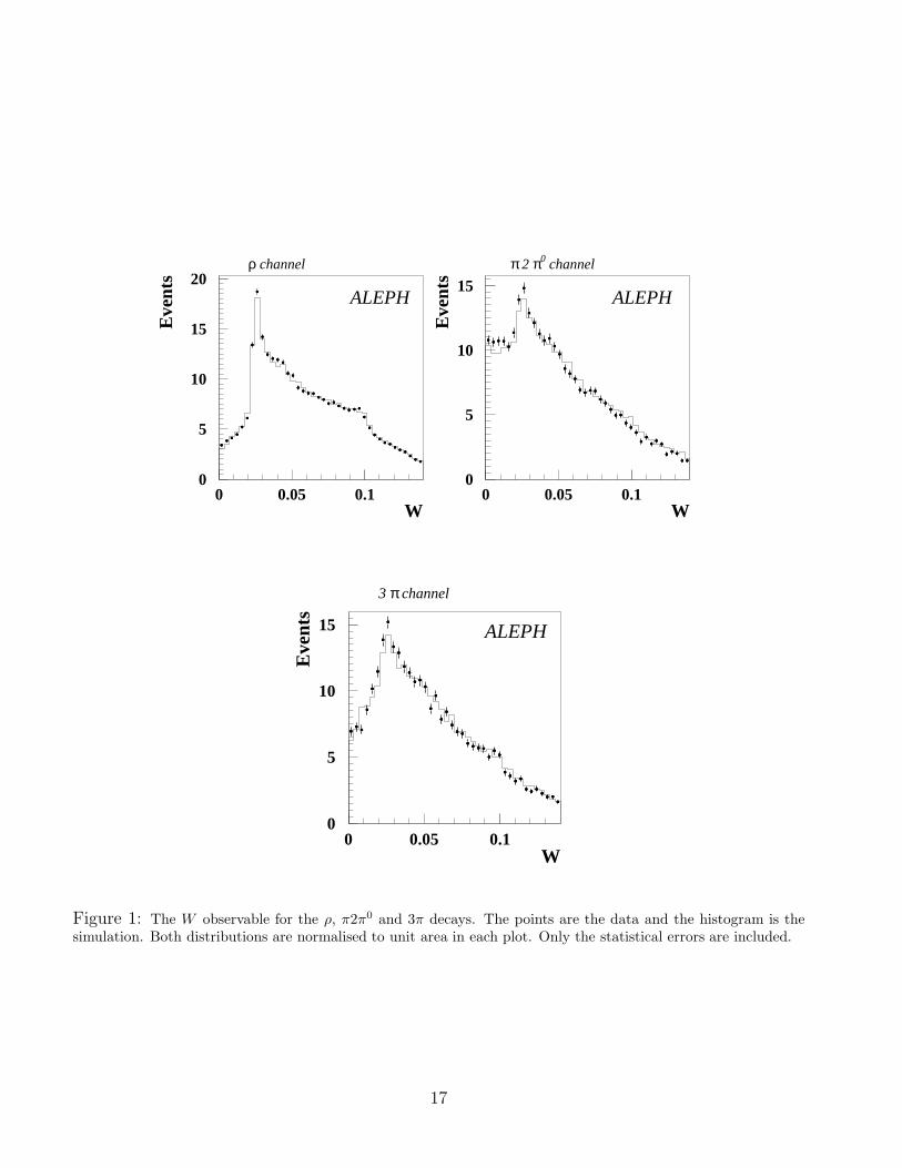
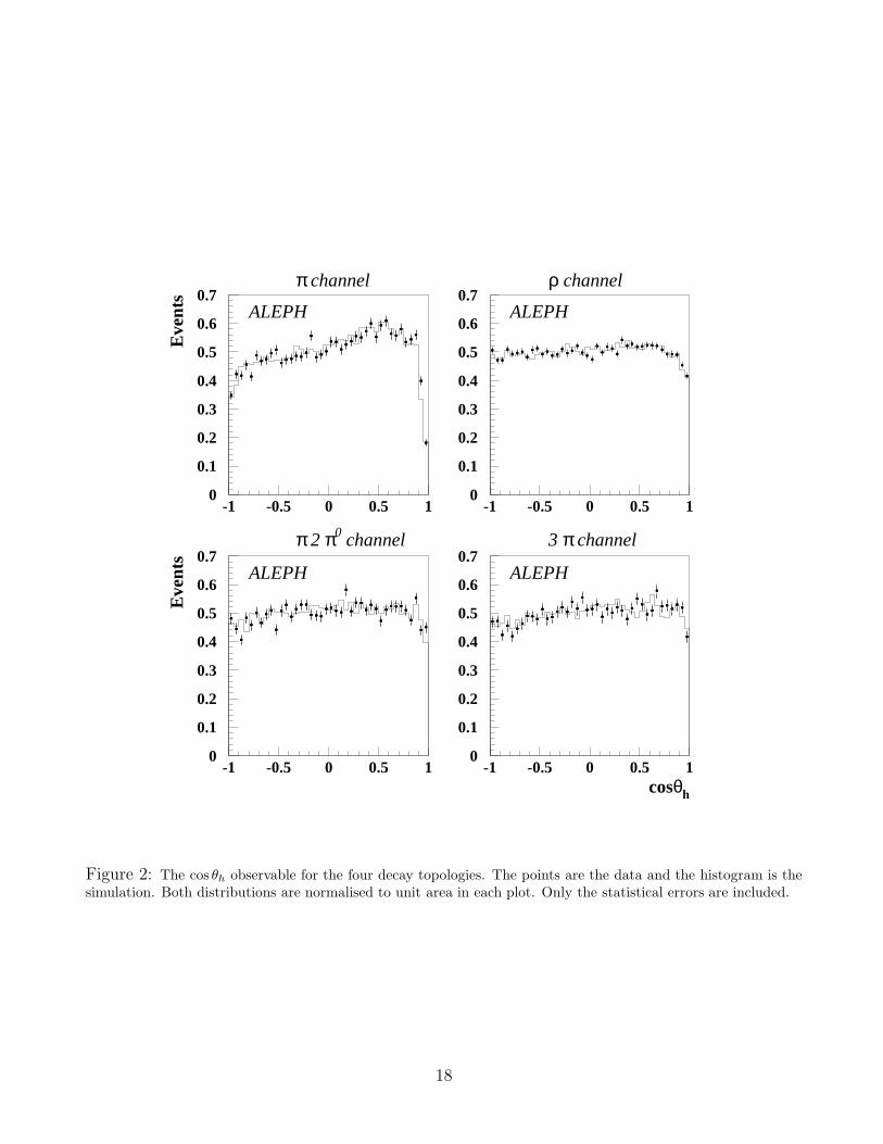
) are the polar and azimuthal angles of thepolarimeters of each τ , in the reference frame introduced in Section 2.1. The above likelihood isalso a function of the centre-of-mass energy. The distributions of the hemisphere observables Wand cos θh are presented in Figs. 1 and 2.

This likelihood fulfills the normalisation condition∑

ij

∫

Lij(µτ , dτ |θτ ,W1, cos θh1, φh1

,W2, cos θh2, φh2

)dX1dX2 = 1 . (14)

This is the integral over all possible decay parameters and all possible decay topologies ij for agiven e+e− → τ+τ− event. The normalisation is such that the likelihood depends only upon thenet spin polarisation of the produced τ pairs, and not upon R00 = dσ/d cos θτ .

3 Apparatus

The ALEPH detector is described in detail in [17] and its performance in [18].

Charged particles are measured with a high resolution silicon vertex detector (VDET), acylindrical drift chamber (ITC), and a large time projection chamber (TPC). The momentumresolution in the axial magnetic field of 1.5 T provided by a superconducting solenoid is ∆p/p2 =0.6 × 10−3(GeV/c)−1 for high momentum tracks. The impact parameter resolutions for highmomentum tracks with hits in all three subdetectors are σrφ = 23µm and σz = 28µm.

The tracking devices are surrounded by the electromagnetic calorimeter (ECAL), which is ahighly segmented lead/proportional-wire-chamber calorimeter. The calorimeter is read out viacathode pads arranged in projective towers covering 0.9◦ × 0.9◦ in solid angle and summing thedeposited energy in three sections of depth. A second readout is provided by the signals from the

anode wires. The energy resolution is σ/E = 0.009 + 0.18/√

E(GeV).

The ECAL is inside the solenoid, which is followed by the hadron calorimeter (HCAL).Hadronic showers are sampled by 23 planes of streamer tubes giving a digital hit pattern andan analog signal on pads, which are also arranged in projective towers. This calorimeter is usedin this analysis to discriminate between pions and muons. Outside the HCAL there are two layersof muon chambers providing additional information for µ identification.

4 Data analysis

4.1 Selection and decay classification

Events from Z → τ+τ− are retained using a global selection in which each event is divided intotwo hemispheres along the thrust axis. The selection is that used in the ALEPH measurementof Pτ (cos θτ ) with the τ direction method [9]. Additional information can be found in [8] andreferences therein.

The charged particle identification is based on a likelihood method which assigns a set ofprobabilities to each particle. A detailed description of the method can be found in Refs. [6, 7].

5

The probability set for each particle is obtained from (i) the specific ionisation dE/dx in the TPC,(ii) the longitudinal and transverse shower profiles in ECAL near the extrapolated track and (iii)the energy and average shower width in HCAL, together with the number out of the last ten ofHCAL planes that fired and the number of hits in the muon chambers.

The photon and π0 reconstruction is performed with a likelihood method which firstdistinguishes between genuine and fake photons produced by hadronic interactions in ECAL or byelectromagnetic shower fluctuations [8]. All photon pairs in each hemisphere are then assigned aprobability of being generated by a π0. High energy π0 with overlapping showers are reconstructedthrough an analysis of the spatial energy deposition in the ECAL towers. All the remaining singlephotons are considered and those with a high probability of being a genuine photon are selected asπ0 candidates. Finally, photon conversions are identified following the procedure described in [8].They are added to the list of good photons and are included in the π0 reconstruction.

The τ decay classification depends on the number of charged tracks and their identification, andon the number of reconstructed π0. It follows the classification for the measurement of Pτ (cos θτ )with the τ direction method, described in [9] and the references therein.

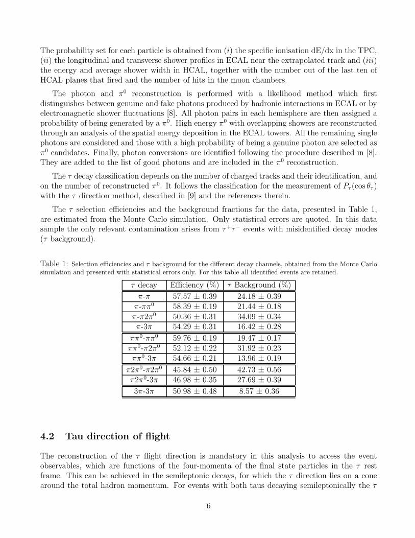
The τ selection efficiencies and the background fractions for the data, presented in Table 1,are estimated from the Monte Carlo simulation. Only statistical errors are quoted. In this datasample the only relevant contamination arises from τ+τ− events with misidentified decay modes(τ background).

Table 1: Selection efficiencies and τ background for the different decay channels, obtained from the Monte Carlosimulation and presented with statistical errors only. For this table all identified events are retained.

τ decay Efficiency (%) τ Background (%)

π-π 57.57 ± 0.39 24.18 ± 0.39π-ππ0 58.39 ± 0.19 21.44 ± 0.18π-π2π0 50.36 ± 0.31 34.09 ± 0.34π-3π 54.29 ± 0.31 16.42 ± 0.28

ππ0-ππ0 59.76 ± 0.19 19.47 ± 0.17ππ0-π2π0 52.12 ± 0.22 31.92 ± 0.23ππ0-3π 54.66 ± 0.21 13.96 ± 0.19

π2π0-π2π0 45.84 ± 0.50 42.73 ± 0.56π2π0-3π 46.98 ± 0.35 27.69 ± 0.39

3π-3π 50.98 ± 0.48 8.57 ± 0.36

4.2 Tau direction of flight

The reconstruction of the τ flight direction is mandatory in this analysis to access the eventobservables, which are functions of the four-momenta of the final state particles in the τ restframe. This can be achieved in the semileptonic decays, for which the τ direction lies on a conearound the total hadron momentum. For events with both taus decaying semileptonically the τ

6

direction lies along one of the intersection lines of the two reconstructed cones in the case that thetaus are produced back-to-back, with equal energies given by

√s/2, and mντ = mντ = 0. However,

the two cones may not intersect due to detector effects or radiation. If the cones intersect, theevent is considered twice using either solution. If the cones do not intersect, the particle momentaare fluctuated within their measurement errors and the event is accepted if the cones intersect ina minimum number of trials; the average direction is then used [9].

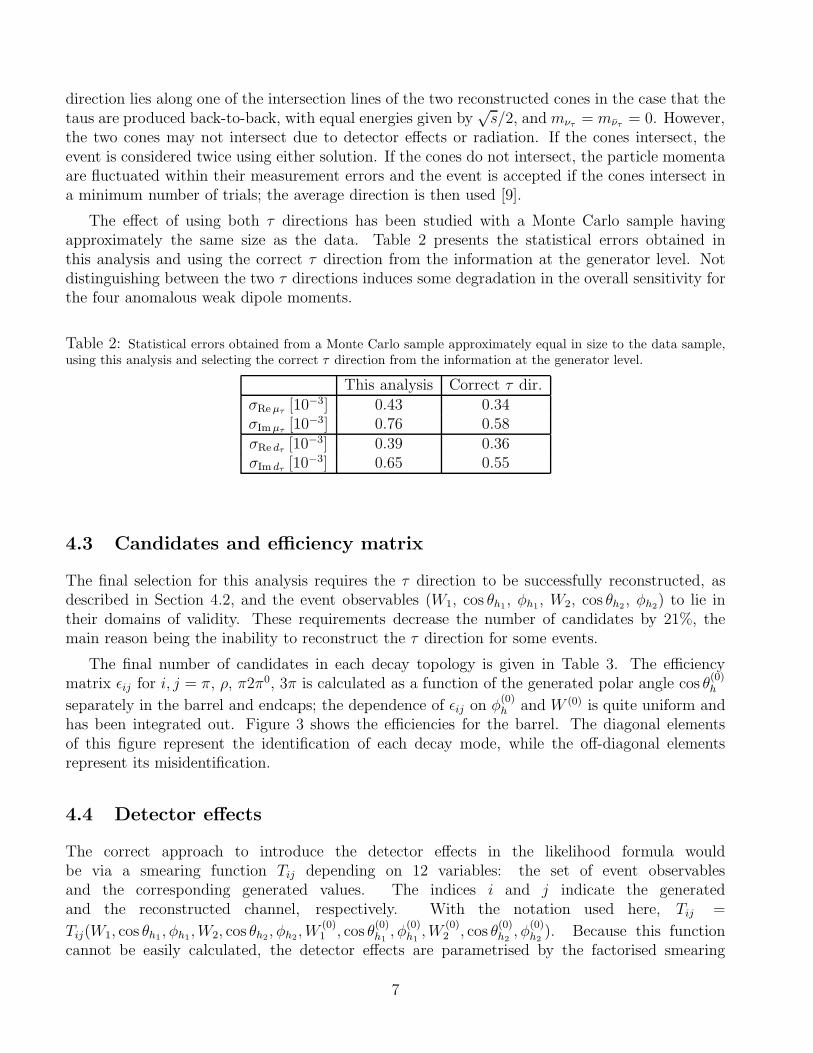
The effect of using both τ directions has been studied with a Monte Carlo sample havingapproximately the same size as the data. Table 2 presents the statistical errors obtained inthis analysis and using the correct τ direction from the information at the generator level. Notdistinguishing between the two τ directions induces some degradation in the overall sensitivity forthe four anomalous weak dipole moments.

Table 2: Statistical errors obtained from a Monte Carlo sample approximately equal in size to the data sample,using this analysis and selecting the correct τ direction from the information at the generator level.

This analysis Correct τ dir.σReµτ

[10−3] 0.43 0.34σImµτ

[10−3] 0.76 0.58σRe dτ [10

−3] 0.39 0.36σIm dτ [10

−3] 0.65 0.55

4.3 Candidates and efficiency matrix

The final selection for this analysis requires the τ direction to be successfully reconstructed, asdescribed in Section 4.2, and the event observables (W1, cos θh1

, φh1, W2, cos θh2

, φh2) to lie in

their domains of validity. These requirements decrease the number of candidates by 21%, themain reason being the inability to reconstruct the τ direction for some events.

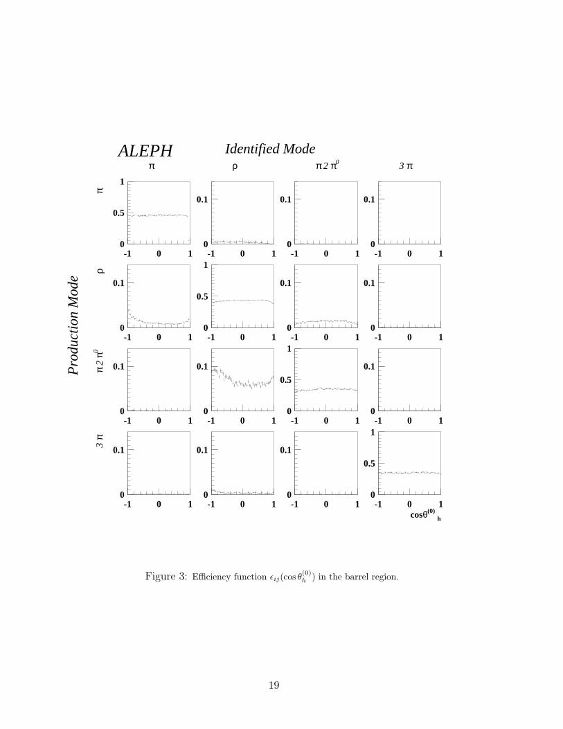
The final number of candidates in each decay topology is given in Table 3. The efficiencymatrix ǫij for i, j = π, ρ, π2π0, 3π is calculated as a function of the generated polar angle cos θ

(0)h

separately in the barrel and endcaps; the dependence of ǫij on φ(0)h and W (0) is quite uniform and

has been integrated out. Figure 3 shows the efficiencies for the barrel. The diagonal elementsof this figure represent the identification of each decay mode, while the off-diagonal elementsrepresent its misidentification.

4.4 Detector effects

The correct approach to introduce the detector effects in the likelihood formula wouldbe via a smearing function Tij depending on 12 variables: the set of event observablesand the corresponding generated values. The indices i and j indicate the generatedand the reconstructed channel, respectively. With the notation used here, Tij =

Tij(W1, cos θh1, φh1

,W2, cos θh2, φh2

,W(0)1 , cos θ

(0)h1, φ

(0)h1,W

(0)2 , cos θ

(0)h2, φ

(0)h2). Because this function

cannot be easily calculated, the detector effects are parametrised by the factorised smearing

7

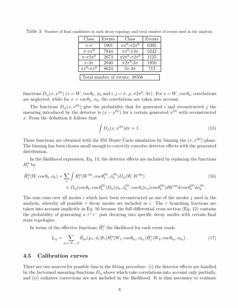
Table 3: Number of final candidates in each decay topology and total number of events used in the analysis.

Class Events Class Events

π-π 1901 ππ0-π2π0 6395π-ππ0 7844 ππ0-π3π 5242π-π2π0 2673 π2π0-π2π0 1125π-3π 2040 π2π0-3π 1950

ππ0-ππ0 8624 3π-3π 712

Total number of events: 38506

functions Dij(x, x(0)) (x = W , cos θh, φh and i, j = π, ρ, π2π0, 3π). For x = W , cos θh, correlations

are neglected, while for x = cos θh, φh, the correlations are taken into account.

The functions Dij(x, x(0)) give the probability that for generated i and reconstructed j the

smearing introduced by the detector is (x − x(0)) for a certain generated x(0) with reconstructedx. From the definition it follows that

∫

Dij(x, x(0))dx = 1 . (15)

These functions are obtained with the SM Monte Carlo simulation by binning the (x, x(0)) plane.The binning has been chosen small enough to correctly convolve detector effects with the generateddistribution.

In the likelihood expression, Eq. 13, the detector effects are included by replacing the functionsHµ

i by

Hµj (W, cos θh, φh) =

∑

i

∫

Hµi (W

(0), cos θ(0)h , φ

(0)h )Dij(W,W (0)) (16)

×Dij(cos θh, cos θ(0)h )Dij(φh, φ

(0)h , cos θh)ǫij(cos θ

(0)h )dW (0)d cos θ

(0)h dφ

(0)h .

The sum runs over all modes i which have been reconstructed as one of the modes j used in theanalysis, whereby all possible τ decay modes are included in i. The τ branching fractions aretaken into account implicitly in Eq. 16 because the full differential cross section (Eq. 12) containsthe probability of generating a τ+τ− pair decaying into specific decay modes with certain finalstate topologies.

In terms of the effective functions Hµi the likelihood for each event reads

Lij =∑

µ,ν=0,...,3

Rµν(µτ , dτ |θτ )Hµi (W1, cos θh1

, φh1)Hν

j (W2, cos θh2, φh2

) . (17)

4.5 Calibration curves

There are two sources for possible bias in the fitting procedure: (i) the detector effects are handledby the factorised smearing functions Dij above which take correlations into account only partially,and (ii) radiative corrections are not included in the likelihood. It is thus necessary to evaluate

8

the adequacy of the fitting process. This is done with the SCOT Monte Carlo program [19],interfaced with TAUOLA for the τ decays and with the full detector simulation. The programSCOT describes e+e− → τ+τ− production at an energy around the Z peak at tree level. Itincludes the anomalous weak dipole moments and all τ spin effects. The initial state radiation isincluded by adding a simple radiator function [20].

The checks are performed by generating various Monte Carlo samples with different values ofthe anomalous weak dipole moments. The couplings ae, ve, aτ , vτ are set to their SM values. Theanomalous weak dipole moments Reµτ , Imµτ , Re dτ , Im dτ are varied one by one in an adequateregion around zero. The dependence of the reconstructed values on the generated parametersis taken as linear. Significant deviations of the slopes from unity are found for certain decaytopologies, and the offset for Reµτ is not consistent with zero for certain channels. These effectshave been studied and are mostly related to not using the correct τ direction and to backgroundeffects. In this analysis, this calibration for each anomalous weak dipole moment and decaytopology is taken into account to obtain the corresponding individual measurements. The slopes,offsets and χ2 of the linear fits are presented in Table 4.

The offsets and slopes were derived with a Monte Carlo program which includes only a firstorder radiator for the initial state bremsstrahlung. The offsets have then been verified withthe KORALZ Monte Carlo program [21] interfaced with the full detector simulation. KORALZdescribes e+e− → τ+τ− production at an energy around the Z peak and with initial statebremsstrahlung corrections up to O(α2), final state O(α) bremsstrahlung and O(α) electroweakcorrections. However, this program contains only longitudinal spin effects (i.e., the productionterms used are R00, R03 and R33) and the anomalous weak dipole moments are set to zero. Tocheck the effect of this approximation, a maximum likelihood fit was built to include the completeR00, R03 and R33 terms and the anomalous parts of the other Rµν terms. The values obtainedfor the four anomalous weak dipole moments for each decay topology are consistent with thecorresponding offsets computed with SCOT and the first order radiator. Table 5 shows the globaldifferences between the offsets of the central values of the four anomalous weak dipole momentswhen using either KORALZ or SCOT. The final results of this analysis are obtained by correctingthe individual measurements according to the KORALZ offsets and the SCOT slopes and byincluding the statistical error of the correction in the systematic uncertainty. The statisticalerror of the SCOT offsets is also included in the systematic uncertainty as these offsets havecontributions from all Rµν terms.

5 Systematic uncertainties

The systematic uncertainty is calculated for each anomalous weak dipole moment and final statedecay topology. The estimates are shown in Tables 6 to 9. The last row of these tables shows thecombined systematic uncertainty from each source taking into account the correlations betweenchannels.

The ECAL effects are related to the uncertainty in the global energy scale and the nonlinearityof the response. The global scale is known at the level of 0.25%, through the calibration withBhabha events. Global variations have been applied to each ECAL module and the effect ispropagated to the fitted parameters. The nonlinearity of the response is related to the wire

9

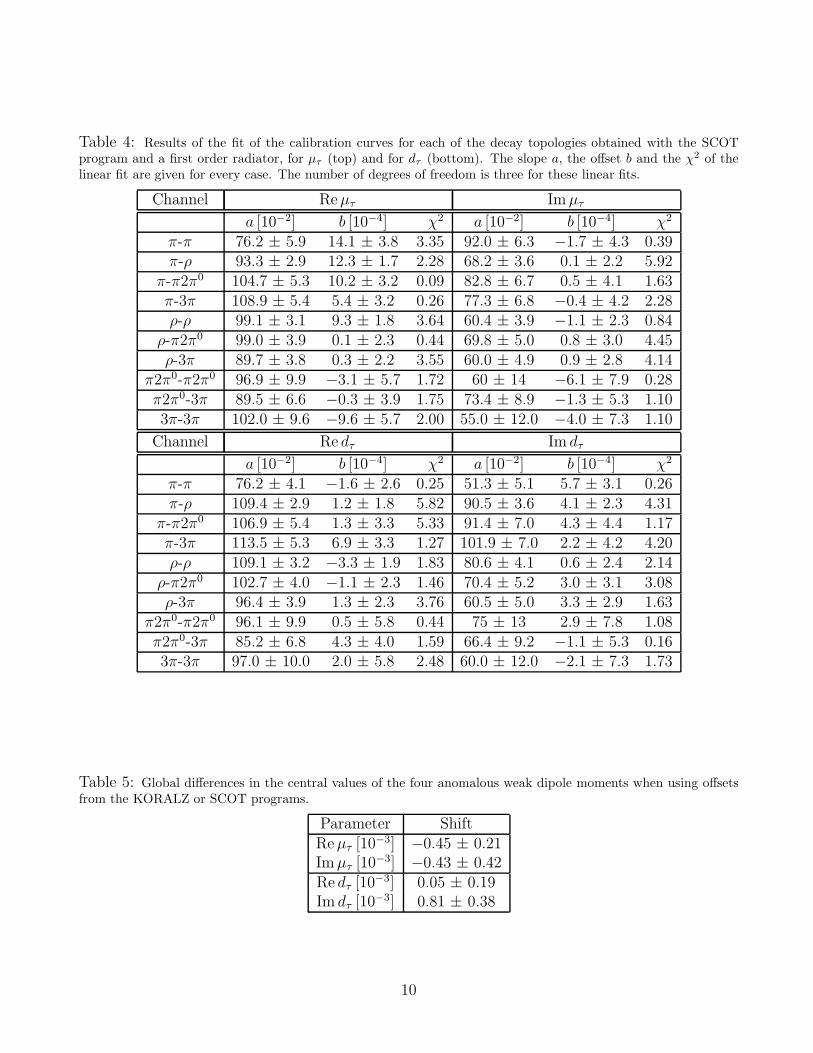
Table 4: Results of the fit of the calibration curves for each of the decay topologies obtained with the SCOTprogram and a first order radiator, for µτ (top) and for dτ (bottom). The slope a, the offset b and the χ2 of thelinear fit are given for every case. The number of degrees of freedom is three for these linear fits.

Channel Reµτ Imµτ

a [10−2] b [10−4] χ2 a [10−2] b [10−4] χ2

π-π 76.2 ± 5.9 14.1 ± 3.8 3.35 92.0 ± 6.3 −1.7 ± 4.3 0.39π-ρ 93.3 ± 2.9 12.3 ± 1.7 2.28 68.2 ± 3.6 0.1 ± 2.2 5.92

π-π2π0 104.7 ± 5.3 10.2 ± 3.2 0.09 82.8 ± 6.7 0.5 ± 4.1 1.63π-3π 108.9 ± 5.4 5.4 ± 3.2 0.26 77.3 ± 6.8 −0.4 ± 4.2 2.28ρ-ρ 99.1 ± 3.1 9.3 ± 1.8 3.64 60.4 ± 3.9 −1.1 ± 2.3 0.84

ρ-π2π0 99.0 ± 3.9 0.1 ± 2.3 0.44 69.8 ± 5.0 0.8 ± 3.0 4.45ρ-3π 89.7 ± 3.8 0.3 ± 2.2 3.55 60.0 ± 4.9 0.9 ± 2.8 4.14

π2π0-π2π0 96.9 ± 9.9 −3.1 ± 5.7 1.72 60 ± 14 −6.1 ± 7.9 0.28π2π0-3π 89.5 ± 6.6 −0.3 ± 3.9 1.75 73.4 ± 8.9 −1.3 ± 5.3 1.103π-3π 102.0 ± 9.6 −9.6 ± 5.7 2.00 55.0 ± 12.0 −4.0 ± 7.3 1.10

Channel Re dτ Im dτ

a [10−2] b [10−4] χ2 a [10−2] b [10−4] χ2

π-π 76.2 ± 4.1 −1.6 ± 2.6 0.25 51.3 ± 5.1 5.7 ± 3.1 0.26π-ρ 109.4 ± 2.9 1.2 ± 1.8 5.82 90.5 ± 3.6 4.1 ± 2.3 4.31

π-π2π0 106.9 ± 5.4 1.3 ± 3.3 5.33 91.4 ± 7.0 4.3 ± 4.4 1.17π-3π 113.5 ± 5.3 6.9 ± 3.3 1.27 101.9 ± 7.0 2.2 ± 4.2 4.20ρ-ρ 109.1 ± 3.2 −3.3 ± 1.9 1.83 80.6 ± 4.1 0.6 ± 2.4 2.14

ρ-π2π0 102.7 ± 4.0 −1.1 ± 2.3 1.46 70.4 ± 5.2 3.0 ± 3.1 3.08ρ-3π 96.4 ± 3.9 1.3 ± 2.3 3.76 60.5 ± 5.0 3.3 ± 2.9 1.63

π2π0-π2π0 96.1 ± 9.9 0.5 ± 5.8 0.44 75 ± 13 2.9 ± 7.8 1.08π2π0-3π 85.2 ± 6.8 4.3 ± 4.0 1.59 66.4 ± 9.2 −1.1 ± 5.3 0.163π-3π 97.0 ± 10.0 2.0 ± 5.8 2.48 60.0 ± 12.0 −2.1 ± 7.3 1.73

Table 5: Global differences in the central values of the four anomalous weak dipole moments when using offsetsfrom the KORALZ or SCOT programs.

Parameter ShiftReµτ [10

−3] −0.45 ± 0.21Imµτ [10

−3] −0.43 ± 0.42Re dτ [10

−3] 0.05 ± 0.19Im dτ [10

−3] 0.81 ± 0.38

10

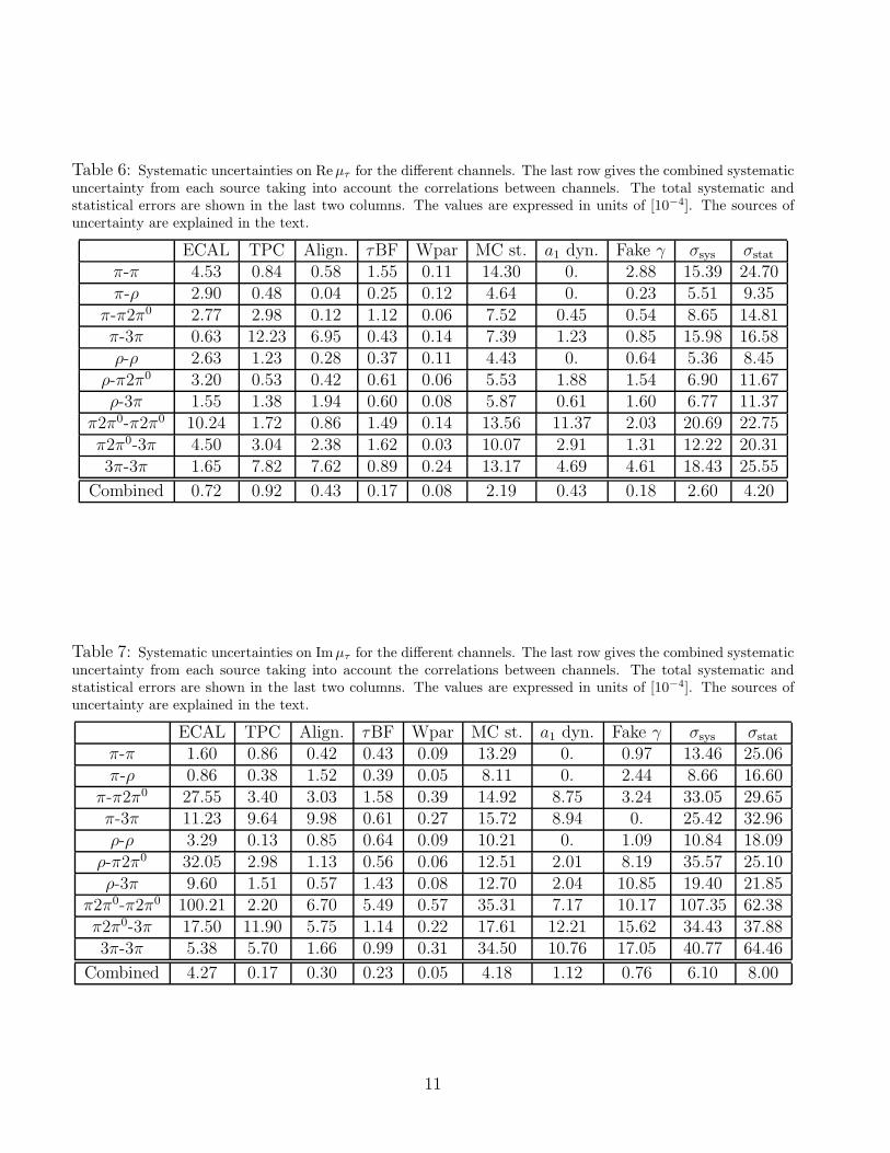
Table 6: Systematic uncertainties on Reµτ for the different channels. The last row gives the combined systematicuncertainty from each source taking into account the correlations between channels. The total systematic andstatistical errors are shown in the last two columns. The values are expressed in units of [10−4]. The sources ofuncertainty are explained in the text.

ECAL TPC Align. τBF Wpar MC st. a1 dyn. Fake γ σsys σstat

π-π 4.53 0.84 0.58 1.55 0.11 14.30 0. 2.88 15.39 24.70π-ρ 2.90 0.48 0.04 0.25 0.12 4.64 0. 0.23 5.51 9.35

π-π2π0 2.77 2.98 0.12 1.12 0.06 7.52 0.45 0.54 8.65 14.81π-3π 0.63 12.23 6.95 0.43 0.14 7.39 1.23 0.85 15.98 16.58ρ-ρ 2.63 1.23 0.28 0.37 0.11 4.43 0. 0.64 5.36 8.45

ρ-π2π0 3.20 0.53 0.42 0.61 0.06 5.53 1.88 1.54 6.90 11.67ρ-3π 1.55 1.38 1.94 0.60 0.08 5.87 0.61 1.60 6.77 11.37

π2π0-π2π0 10.24 1.72 0.86 1.49 0.14 13.56 11.37 2.03 20.69 22.75π2π0-3π 4.50 3.04 2.38 1.62 0.03 10.07 2.91 1.31 12.22 20.313π-3π 1.65 7.82 7.62 0.89 0.24 13.17 4.69 4.61 18.43 25.55

Combined 0.72 0.92 0.43 0.17 0.08 2.19 0.43 0.18 2.60 4.20

Table 7: Systematic uncertainties on Imµτ for the different channels. The last row gives the combined systematicuncertainty from each source taking into account the correlations between channels. The total systematic andstatistical errors are shown in the last two columns. The values are expressed in units of [10−4]. The sources ofuncertainty are explained in the text.

ECAL TPC Align. τBF Wpar MC st. a1 dyn. Fake γ σsys σstat

π-π 1.60 0.86 0.42 0.43 0.09 13.29 0. 0.97 13.46 25.06π-ρ 0.86 0.38 1.52 0.39 0.05 8.11 0. 2.44 8.66 16.60

π-π2π0 27.55 3.40 3.03 1.58 0.39 14.92 8.75 3.24 33.05 29.65π-3π 11.23 9.64 9.98 0.61 0.27 15.72 8.94 0. 25.42 32.96ρ-ρ 3.29 0.13 0.85 0.64 0.09 10.21 0. 1.09 10.84 18.09

ρ-π2π0 32.05 2.98 1.13 0.56 0.06 12.51 2.01 8.19 35.57 25.10ρ-3π 9.60 1.51 0.57 1.43 0.08 12.70 2.04 10.85 19.40 21.85

π2π0-π2π0 100.21 2.20 6.70 5.49 0.57 35.31 7.17 10.17 107.35 62.38π2π0-3π 17.50 11.90 5.75 1.14 0.22 17.61 12.21 15.62 34.43 37.883π-3π 5.38 5.70 1.66 0.99 0.31 34.50 10.76 17.05 40.77 64.46

Combined 4.27 0.17 0.30 0.23 0.05 4.18 1.12 0.76 6.10 8.00

11

saturation constants of ECAL, which are different in the barrel and endcaps. These saturationconstants have been fluctuated within their nominal errors while keeping the measured energyfixed at MZ/2.

The TPC systematic errors are related to the momentum measurement: (i) an effect due tothe magnetic field acting similarly on positive and negative charged tracks, and (ii) a sagitta effectaffecting oppositely positive and negative tracks. These two effects are calibrated with dimuonevents and the corresponding corrections are applied to the τ data. The systematic errors arethen estimated by varying the corrections within their errors for each year.

The systematic errors in the column labeled “Align.” are due to a possible azimuthal tiltbetween the different parts of the detector.

Variations in the τ branching fractions are considered in the τBF column. This systematicuncertainty was determined from its effect on the calibration curves (Section 4.5).

The experimental errors on the weak parameters sin2 θW and MZ are propagated to the fittedvalues. Other weak parameters have negligible effect on the measurements. These effects aresummarised in the column labeled “Wpar”.

The finite Monte Carlo statistics also causes systematic uncertainties. The most relevantstatistical uncertainty is for the KORALZ offsets. The statistical error of the offsets and slopesobtained with SCOT and the first order radiator (Table 4) are also taken into account. Finally,the statistical error in the calculation of the efficiency matrix is also considered. These effects areshown under the column “MC st.”.

Table 8: Systematic uncertainties on Re dτ for the different channels. The last row gives the combined systematicuncertainty from each source taking into account the correlations between channels. The total systematic andstatistical errors are shown in the last two columns. The values are expressed in units of [10−4]. The sources ofuncertainty are explained in the text.

ECAL TPC Align. τBF Wpar MC st. a1 dyn. Fake γ σsys σstat

π-π 1.27 0.58 0.09 0.77 0.12 8.33 0. 0.16 8.48 15.61π-ρ 0.18 0.40 0.61 0.35 0.04 3.91 0. 4.51 6.03 7.94

π-π2π0 8.38 1.73 1.58 1.78 0.09 7.68 3.36 3.21 12.63 15.34π-3π 1.36 0.57 0.02 0.27 0.02 7.22 2.71 1.00 7.92 15.05ρ-ρ 0.53 0.35 0.49 0.38 0.04 4.18 0. 0.17 4.28 8.04

ρ-π2π0 1.45 1.68 0.63 0.79 0.08 5.39 0.79 2.63 6.52 10.89ρ-3π 5.37 1.68 0.79 0.45 0. 5.56 3.00 2.26 8.80 10.89

π2π0-π2π0 8.75 2.00 1.10 1.71 0.07 13.35 8.18 9.44 20.47 29.74π2π0-3π 5.26 12.07 10.96 2.56 0.05 10.39 4.88 3.75 21.11 21.653π-3π 1.91 4.75 4.70 1.64 0.12 14.06 5.34 2.25 16.80 29.39

Combined 0.41 0.29 0.26 0.17 0.02 1.94 0.90 0.50 2.30 3.90

The a1 decay dynamics are not well described theoretically. The impact of this was evaluatedin the past [22] by implementing several models in the analysis [23]. The implementation of thosemodels is much more difficult in the present analysis. The uncertainty is estimated by means ofthree models: the Kuhn & Santamaria (KS) model [24] (used in the fitting formula), the Feindt

12

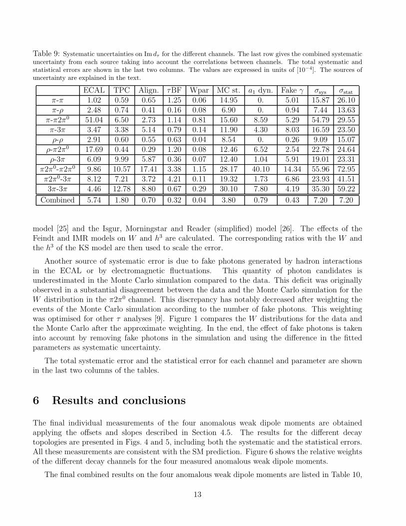
Table 9: Systematic uncertainties on Im dτ for the different channels. The last row gives the combined systematicuncertainty from each source taking into account the correlations between channels. The total systematic andstatistical errors are shown in the last two columns. The values are expressed in units of [10−4]. The sources ofuncertainty are explained in the text.

ECAL TPC Align. τBF Wpar MC st. a1 dyn. Fake γ σsys σstat

π-π 1.02 0.59 0.65 1.25 0.06 14.95 0. 5.01 15.87 26.10π-ρ 2.48 0.74 0.41 0.16 0.08 6.90 0. 0.94 7.44 13.63

π-π2π0 51.04 6.50 2.73 1.14 0.81 15.60 8.59 5.29 54.79 29.55π-3π 3.47 3.38 5.14 0.79 0.14 11.90 4.30 8.03 16.59 23.50ρ-ρ 2.91 0.60 0.55 0.63 0.04 8.54 0. 0.26 9.09 15.07

ρ-π2π0 17.69 0.44 0.29 1.20 0.08 12.46 6.52 2.54 22.78 24.64ρ-3π 6.09 9.99 5.87 0.36 0.07 12.40 1.04 5.91 19.01 23.31

π2π0-π2π0 9.86 10.57 17.41 3.38 1.15 28.17 40.10 14.34 55.96 72.95π2π0-3π 8.12 7.21 3.72 4.21 0.11 19.32 1.73 6.86 23.93 41.513π-3π 4.46 12.78 8.80 0.67 0.29 30.10 7.80 4.19 35.30 59.22

Combined 5.74 1.80 0.70 0.32 0.04 3.80 0.79 0.43 7.20 7.20

model [25] and the Isgur, Morningstar and Reader (simplified) model [26]. The effects of theFeindt and IMR models on W and h3 are calculated. The corresponding ratios with the W andthe h3 of the KS model are then used to scale the error.

Another source of systematic error is due to fake photons generated by hadron interactionsin the ECAL or by electromagnetic fluctuations. This quantity of photon candidates isunderestimated in the Monte Carlo simulation compared to the data. This deficit was originallyobserved in a substantial disagreement between the data and the Monte Carlo simulation for theW distribution in the π2π0 channel. This discrepancy has notably decreased after weighting theevents of the Monte Carlo simulation according to the number of fake photons. This weightingwas optimised for other τ analyses [9]. Figure 1 compares the W distributions for the data andthe Monte Carlo after the approximate weighting. In the end, the effect of fake photons is takeninto account by removing fake photons in the simulation and using the difference in the fittedparameters as systematic uncertainty.

The total systematic error and the statistical error for each channel and parameter are shownin the last two columns of the tables.

6 Results and conclusions

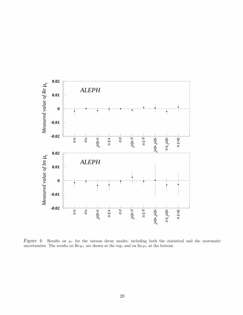
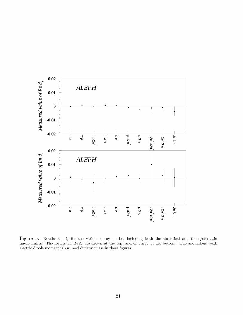
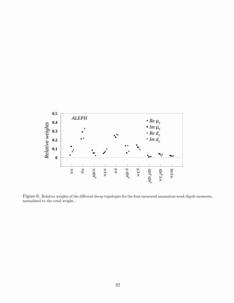
The final individual measurements of the four anomalous weak dipole moments are obtainedapplying the offsets and slopes described in Section 4.5. The results for the different decaytopologies are presented in Figs. 4 and 5, including both the systematic and the statistical errors.All these measurements are consistent with the SM prediction. Figure 6 shows the relative weightsof the different decay channels for the four measured anomalous weak dipole moments.

The final combined results on the four anomalous weak dipole moments are listed in Table 10,

13

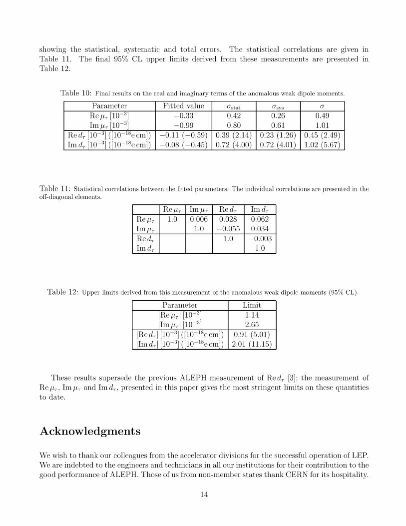
showing the statistical, systematic and total errors. The statistical correlations are given inTable 11. The final 95% CL upper limits derived from these measurements are presented inTable 12.

Table 10: Final results on the real and imaginary terms of the anomalous weak dipole moments.

Parameter Fitted value σstat σsys σReµτ [10

−3] −0.33 0.42 0.26 0.49Imµτ [10

−3] −0.99 0.80 0.61 1.01Re dτ [10

−3] ([10−18e cm]) −0.11 (−0.59) 0.39 (2.14) 0.23 (1.26) 0.45 (2.49)Im dτ [10

−3] ([10−18e cm]) −0.08 (−0.45) 0.72 (4.00) 0.72 (4.01) 1.02 (5.67)

Table 11: Statistical correlations between the fitted parameters. The individual correlations are presented in theoff-diagonal elements.

Reµτ Imµτ Re dτ Im dτReµτ 1.0 0.006 0.028 0.062Imµτ 1.0 −0.055 0.034Re dτ 1.0 −0.003Im dτ 1.0

Table 12: Upper limits derived from this measurement of the anomalous weak dipole moments (95% CL).

Parameter Limit|Reµτ | [10−3] 1.14|Imµτ | [10−3] 2.65

|Re dτ | [10−3] ([10−18e cm]) 0.91 (5.01)|Im dτ | [10−3] ([10−18e cm]) 2.01 (11.15)

These results supersede the previous ALEPH measurement of Re dτ [3]; the measurement ofReµτ , Imµτ and Im dτ , presented in this paper gives the most stringent limits on these quantitiesto date.

Acknowledgments

We wish to thank our colleagues from the accelerator divisions for the successful operation of LEP.We are indebted to the engineers and technicians in all our institutions for their contribution to thegood performance of ALEPH. Those of us from non-member states thank CERN for its hospitality.

14

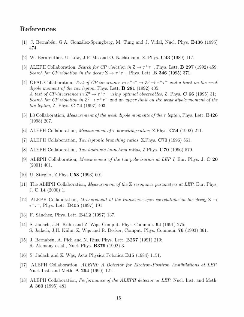
References

[1] J. Bernabeu, G.A. Gonzalez-Springberg, M. Tung and J. Vidal, Nucl. Phys. B436 (1995)474.

[2] W. Bernreuther, U. Low, J.P. Ma and O. Nachtmann, Z. Phys. C43 (1989) 117.

[3] ALEPH Collaboration, Search for CP violation in Z → τ+τ−, Phys. Lett. B 297 (1992) 459;Search for CP violation in the decay Z → τ+τ−, Phys. Lett. B 346 (1995) 371.

[4] OPAL Collaboration, Test of CP-invariance in e+e− → Z0 → τ+τ− and a limit on the weak

dipole moment of the tau lepton, Phys. Lett. B 281 (1992) 405;A test of CP-invariance in Z0 → τ+τ− using optimal observables, Z. Phys. C 66 (1995) 31;Search for CP violation in Z0 → τ+τ− and an upper limit on the weak dipole moment of the

tau lepton, Z. Phys. C 74 (1997) 403.

[5] L3 Collaboration, Measurement of the weak dipole moments of the τ lepton, Phys. Lett. B426

(1998) 207.

[6] ALEPH Collaboration, Measurement of τ branching ratios, Z.Phys. C54 (1992) 211.

[7] ALEPH Collaboration, Tau leptonic branching ratios, Z.Phys. C70 (1996) 561.

[8] ALEPH Collaboration, Tau hadronic branching ratios, Z.Phys. C70 (1996) 579.

[9] ALEPH Collaboration, Measurement of the tau polarisation at LEP I, Eur. Phys. J. C 20

(2001) 401.

[10] U. Stiegler, Z.Phys.C58 (1993) 601.

[11] The ALEPH Collaboration, Measurement of the Z resonance parameters at LEP, Eur. Phys.J. C 14 (2000) 1.

[12] ALEPH Collaboration, Measurement of the transverse spin correlations in the decay Z →τ+τ−, Phys. Lett. B405 (1997) 191.

[13] F. Sanchez, Phys. Lett. B412 (1997) 137.

[14] S. Jadach, J.H. Kuhn and Z. Was, Comput. Phys. Commun. 64 (1991) 275;S. Jadach, J.H. Kuhn, Z. Was and R. Decker, Comput. Phys. Commun. 76 (1993) 361.

[15] J. Bernabeu, A. Pich and N. Rius, Phys. Lett. B257 (1991) 219;R. Alemany et al., Nucl. Phys. B379 (1992) 3.

[16] S. Jadach and Z. Was, Acta Physica Polonica B15 (1984) 1151.

[17] ALEPH Collaboration, ALEPH: A Detector for Electron-Positron Annihilations at LEP,Nucl. Inst. and Meth. A 294 (1990) 121.

[18] ALEPH Collaboration, Performance of the ALEPH detector at LEP, Nucl. Inst. and Meth.A 360 (1995) 481.

15

[19] U. Stiegler, Comput. Phys. Commun. 81 (1994) 221.

[20] G. Bonneau and F. Martin, Nucl. Phys. B27 (1971) 381;R. Miquel, Radiative corrections to the process e+e− → ννγ, Ph.D. thesis, UniversitatAutonoma de Barcelona (1989).

[21] S. Jadach, Z. Was and B.F.L. Ward, Comput. Phys. Commun. 66 (1991) 276.

[22] ALEPH Collaboration, Improved τ polarization measurement, Z.Phys. C69 (1996) 183.

[23] L. Duflot, Nouvelle methode de mesure de la polarisation du τ . Application au canal τ → a1ντdans l’experience ALEPH, Ph.D. thesis, Universite de Paris-Sud, Centre d’Orsay (1993).

[24] J.H. Kuhn and A. Santamaria, τ decays to pions, Munich preprint MPIPAE/PTh 17/90.

[25] M. Feindt, Z. Phys. C48 (1990) 681.

[26] N. Isgur et al., Phys. Rev. D39 (1989) 1357.

16

W

Eve

nts

ρ channel

ALEPH ALEPH

π 2 π0 channel

W

Eve

nts

0

5

10

15

20

0 0.05 0.10

5

10

15

0 0.05 0.1

W

Eve

nts

3 π channel

ALEPH

0

5

10

15

0 0.05 0.1

Figure 1: The W observable for the ρ, π2π0 and 3π decays. The points are the data and the histogram is thesimulation. Both distributions are normalised to unit area in each plot. Only the statistical errors are included.

17

ALEPH

Eve

nts

π channel ρ channel

π 2 π0 channel 3 π channel

ALEPH

Eve

nts

ALEPH ALEPH

cosθh

0

0.1

0.2

0.3

0.4

0.5

0.6

0.7

-1 -0.5 0 0.5 10

0.1

0.2

0.3

0.4

0.5

0.6

0.7

-1 -0.5 0 0.5 1

0

0.1

0.2

0.3

0.4

0.5

0.6

0.7

-1 -0.5 0 0.5 10

0.1

0.2

0.3

0.4

0.5

0.6

0.7

-1 -0.5 0 0.5 1

Figure 2: The cos θh observable for the four decay topologies. The points are the data and the histogram is thesimulation. Both distributions are normalised to unit area in each plot. Only the statistical errors are included.

18

π

ALEPHπ ρ

Identified Modeπ 2 π0 3 π

ρπ

2 π0

Pro

duct

ion

Mod

e

3 π

cosθ(0) h

0

0.5

1

-1 0 10

0.1

-1 0 10

0.1

-1 0 10

0.1

-1 0 1

0

0.1

-1 0 10

0.5

1

-1 0 10

0.1

-1 0 10

0.1

-1 0 1

0

0.1

-1 0 10

0.1

-1 0 10

0.5

1

-1 0 10

0.1

-1 0 1

0

0.1

-1 0 10

0.1

-1 0 10

0.1

-1 0 10

0.5

1

-1 0 1

Figure 3: Efficiency function ǫij(cos θ(0)h ) in the barrel region.

19

ALEPH

Mea

sure

d va

lue

of R

e µ τ

π π

π ρ

π π2π0

π 3 π

ρ ρ

ρ π2π0

ρ 3 π

π2π0 π2π

0

π2π0 3 π

3π 3 π

ALEPH

Mea

sure

d va

lue

of I

m µ

τ

π π

π ρ

π π2π0

π 3 π

ρ ρ

ρ π2π0

ρ 3 π

π2π0 π2π

0

π2π0 3 π

3π 3 π

-0.02

-0.01

0

0.01

0.02

-0.02

-0.01

0

0.01

0.02

Figure 4: Results on µτ for the various decay modes, including both the statistical and the systematicuncertainties. The results on Reµτ are shown at the top, and on Imµτ at the bottom.

20

ALEPH

Mea

sure

d va

lue

of R

e d τ

π π

π ρ

π π2π0

π 3 π

ρ ρ

ρ π2π0

ρ 3 π

π2π0 π2π

0

π2π0 3 π

3π 3 π

ALEPH

Mea

sure

d va

lue

of I

m d

τ

π π

π ρ

π π2π0

π 3 π

ρ ρ

ρ π2π0

ρ 3 π

π2π0 π2π

0

π2π0 3 π

3π 3 π

-0.02

-0.01

0

0.01

0.02

-0.02

-0.01

0

0.01

0.02

Figure 5: Results on dτ for the various decay modes, including both the statistical and the systematicuncertainties. The results on Re dτ are shown at the top, and on Im dτ at the bottom. The anomalous weakelectric dipole moment is assumed dimensionless in these figures.

21

Re µτIm µτRe dτIm dτ

ALEPH

Rel

ativ

e w

eigh

ts

π π

π ρ

π π2π0

π 3 π

ρ ρ

ρ π2π0

ρ 3 π

π2π0 π2π

0

π2π0 3 π

3π 3 π

0

0.1

0.2

0.3

0.4

0.5

Figure 6: Relative weights of the different decay topologies for the four measured anomalous weak dipole moments,normalised to the total weight.

22