Eric Prebys, FNAL. We consider motion of particles either through a linear structure or in a...

Longitudinal Motion 1Eric Prebys, FNAL

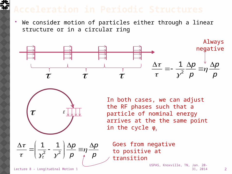
Acceleration in Periodic Structures We consider motion of particles either through a linear structure or

in a circular ring

USPAS, Knoxville, TN, Jan. 20-31, 2014Lecture 8 - Longitudinal Motion 1 2

EIn both cases, we can adjust the RF phases such that a particle of nominal energy arrives at the the same point in the cycle φs

p

p

p

p

2

1

p

p

p

p

t

22

11

Always negative

Goes from negative to positive at transition

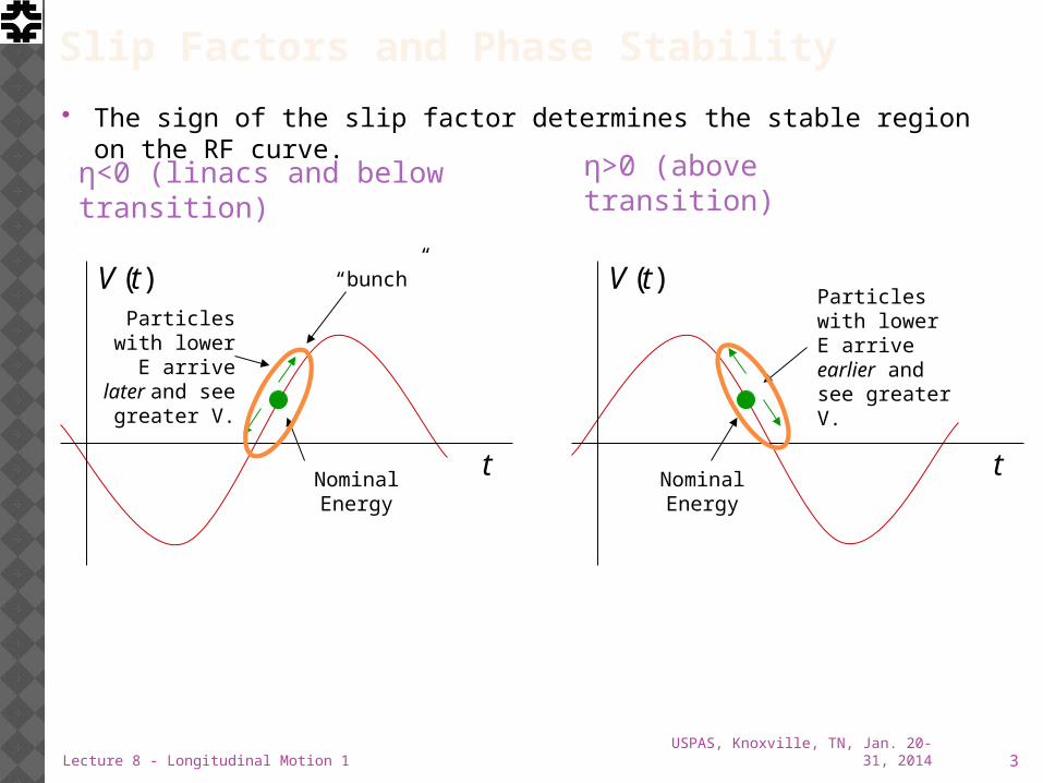
Slip Factors and Phase Stability

The sign of the slip factor determines the stable region on the RF curve.

)(tV

tNominal Energy

Particles with lower E arrive

later and see greater V.

η<0 (linacs and below transition)

)(tV

tNominal Energy

Particles with lower E arrive earlier and see greater V.

“bunch”

USPAS, Knoxville, TN, Jan. 20-31, 2014 3Lecture 8 - Longitudinal Motion 1

η>0 (above transition)

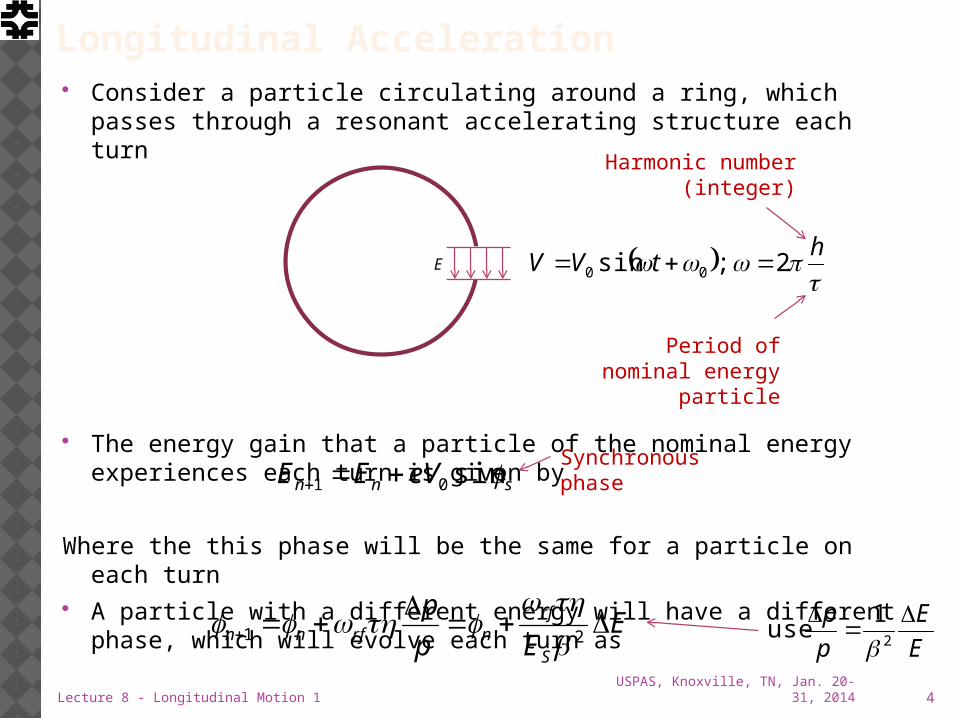
Longitudinal Acceleration Consider a particle circulating around a ring, which passes through

a resonant accelerating structure each turn

The energy gain that a particle of the nominal energy experiences each turn is given by

Where the this phase will be the same for a particle on each turn A particle with a different energy will have a different phase, which

will evolve each turn as


E

htVV 2 ;sin 00

Period of nominal energy particle

Harmonic number (integer)

snn eVEE sin01 Synchronous phase

EEp

p

S

rfnrfnn

21

E

E

p

p

2

1 use

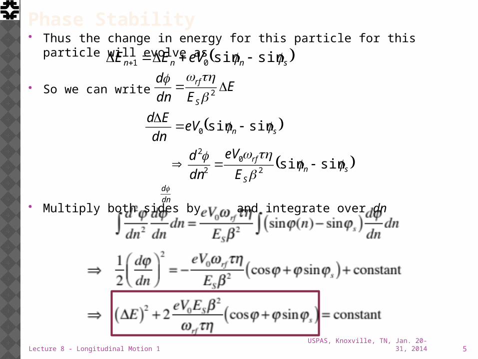
Phase Stability Thus the change in energy for this particle for this particle will

evolve as

So we can write

Multiply both sides by and integrate over dn


snnn eVEE sinsin01

snS

rf

sn

S

rf

E

eV

dn

d

eVdn

Ed

EEdn

d

sinsin

sinsin

2

0

2

2

0

2

dn

d

Synchrotron motion and Synchrotron Tune Going back to our original equation

For small oscillations,

And we have

This is the equation of a harmonic oscillator with


0sinsin2

0

2

2

sn

S

rf

E

eV

dn

d

ssnssn coscossinsin

0cos2

0

2

2

sS

rf

E

eV

dn

d

sS

rfss

S

rfn E

eV

E

eV

cos2

1cos

2

0

2

0

Angular frequency wrt turn (not time)

“synchrotron tune” = number of oscillations per turn (usually <<1)

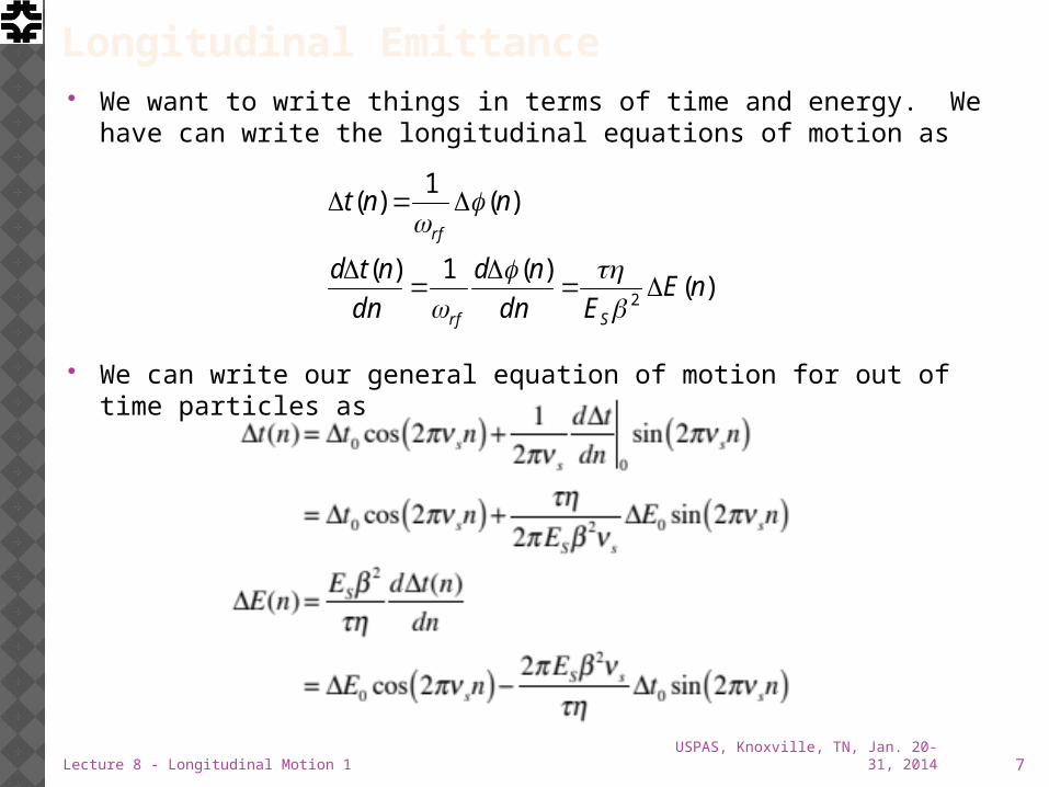
Longitudinal Emittance We want to write things in terms of time and energy. We have can

write the longitudinal equations of motion as

We can write our general equation of motion for out of time particles as


)()(1)(

)(1

)(

2nE

Edn

nd

dn

ntd

nnt

Srf

rf

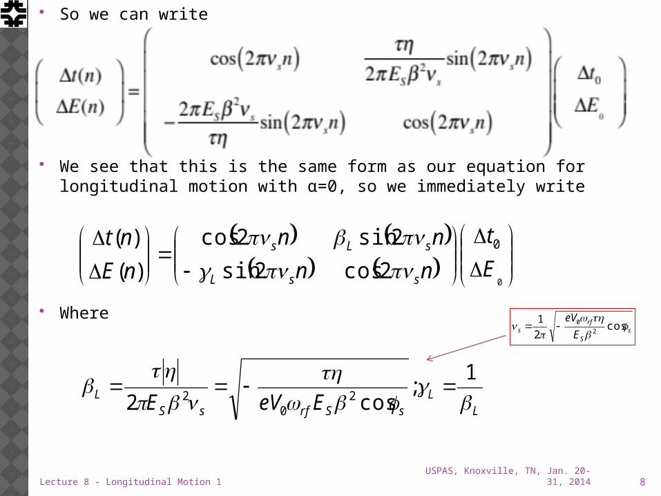
So we can write

We see that this is the same form as our equation for longitudinal motion with α=0, so we immediately write

Where


0

0

2cos2sin

2sin2cos

)(

)(

E

t

nn

nn

nE

nt

ssL

sLs

LL

sSrfsSL EeVE

1

;cos2 2

02

sS

rfs E

eV

cos

2

12

0

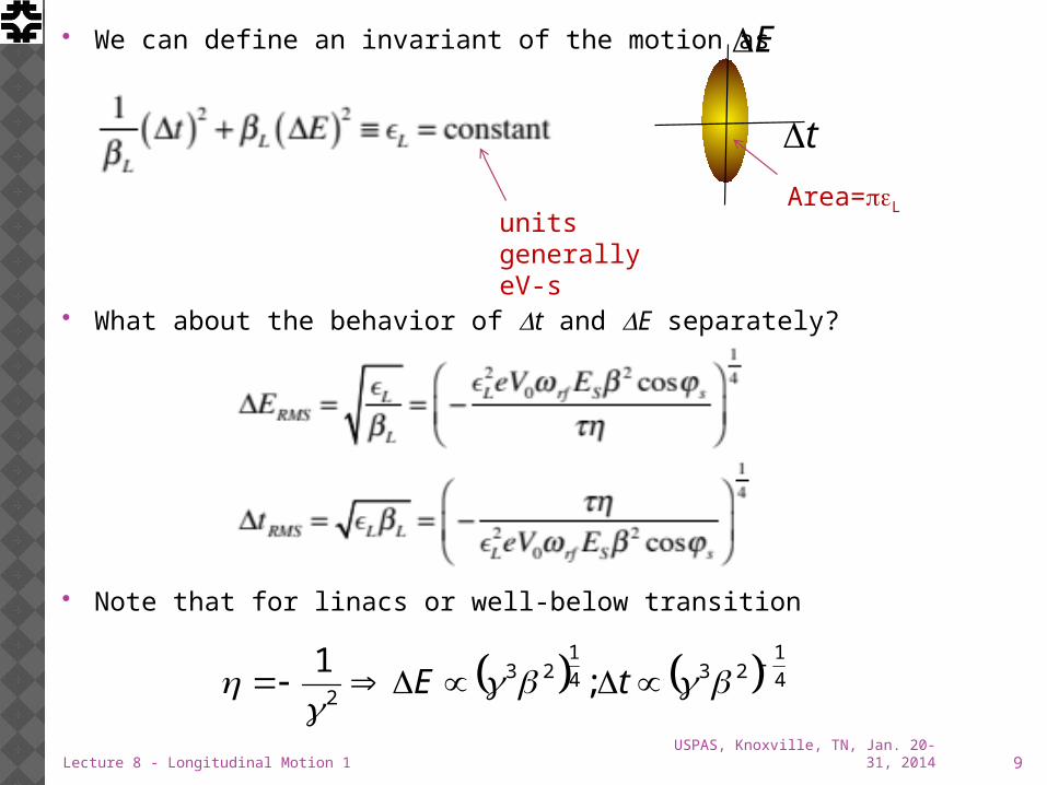
We can define an invariant of the motion as

What about the behavior of t and E separately?

Note that for linacs or well-below transition


t

E

Area= εp Lunits generally eV-s

4

1234

123

2;

1

tE

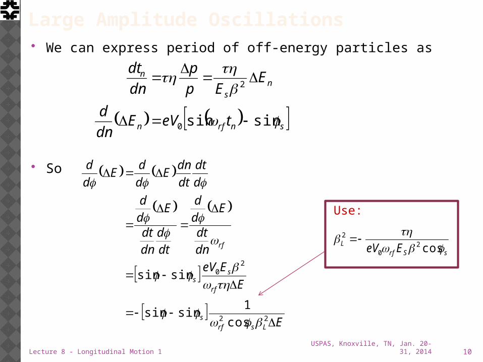
Large Amplitude Oscillations We can express period of off-energy particles as

So


snrfn

ns

n

teVEdn

d

EEp

p

dn

dt

sinsin0

2

E

E

EeV

dndt

Edd

dtd

dndt

Edd

d

dt

dt

dnE

d

dE

d

d

Lsrfs

rf

ss

rf

22

20

cos

1sinsin

sinsin

sSrfL EeV

cos2

0

2

Use:

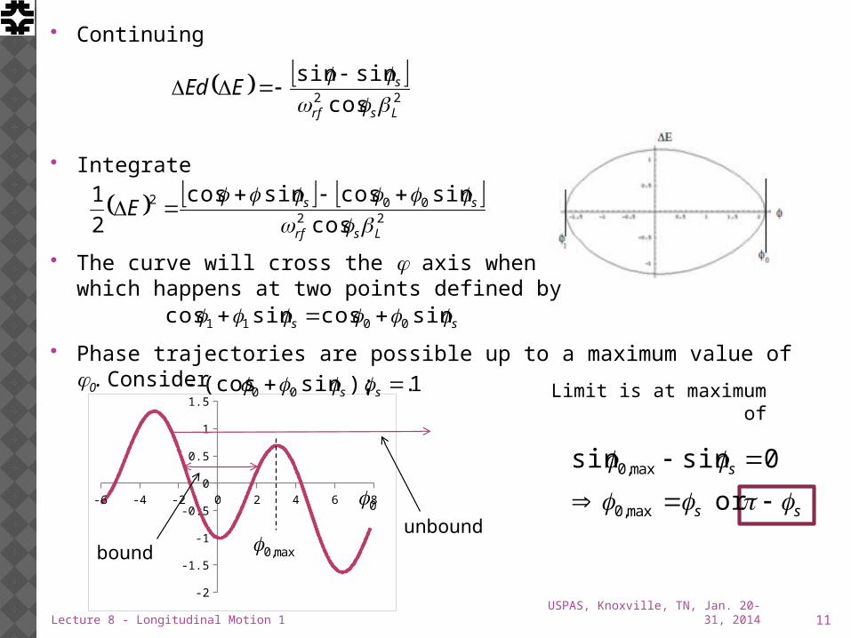
Continuing

Integrate

The curve will cross the φ axis when E=0,which happens at two points defined by

Phase trajectories are possible up to a maximum value of φ0. Consider .


22 cos

sinsin

Lsrf

sEEd

22

002

cos

sincossincos

2

1

Lsrf

ssE

ss sincossincos 0011

-6 -4 -2 0 2 4 6 8

-2

-1.5

-1

-0.5

0

0.5

1

1.51. );sin(cos 00 ss

0

boundunbound

max,0

Limit is at maximum of

ss

s

or

0sinsin

max,0

max,0

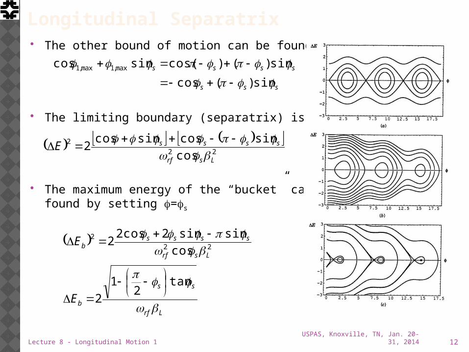
Longitudinal Separatrix The other bound of motion can be found by

The limiting boundary (separatrix) is defined by

The maximum energy of the “bucket” can be found by setting f=fs


sss

ssss

sin)(cos

sin)()cos(sincos max,1max,1

22

2

cos

sincossincos2

Lsrf

ssssE

Lrf

ss

b

Lsrf

ssssb

E

E

tan2

1

2

cos

sinsin2cos22

22

2

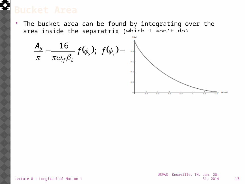
Bucket Area The bucket area can be found by integrating over the area inside

the separatrix (which I won’t do)


ssLrf

b ffA

;

16

Transition Crossing We learned that for a simple FODO lattice

so electron machines are always above transition. Proton machines are often designed to accelerate through

transition. As we go through transition Recall

so these both go to zero at transition. To keep motion stable


T

000

max

max2

0

2

0

cos

cos2

1

E

t

EeV

E

eV

sSrfL

sS

rfs

ss

ss

2n; transitioabove 0cos

20n; transitiobelow 0cos

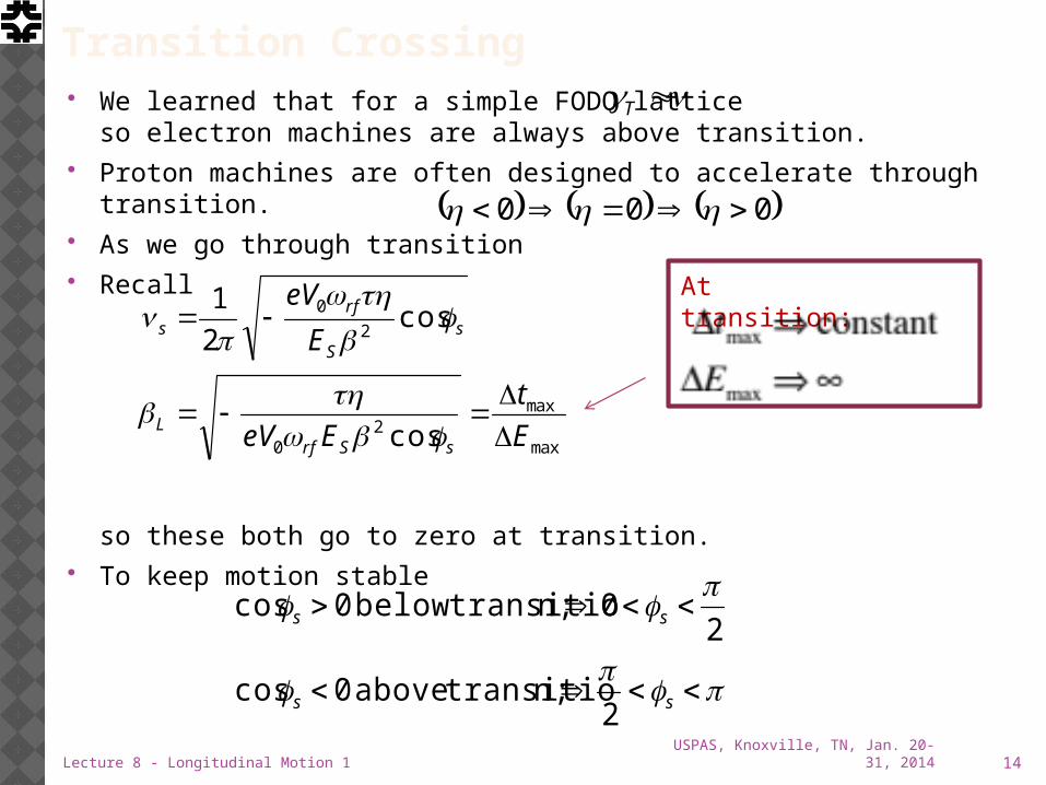
At transition:

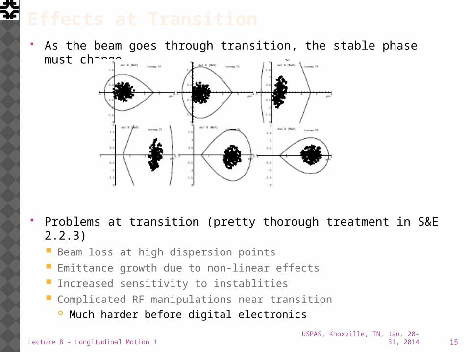
Effects at Transition As the beam goes through transition, the stable phase must

change

Problems at transition (pretty thorough treatment in S&E 2.2.3) Beam loss at high dispersion points Emittance growth due to non-linear effects Increased sensitivity to instablities Complicated RF manipulations near transition

Much harder before digital electronics


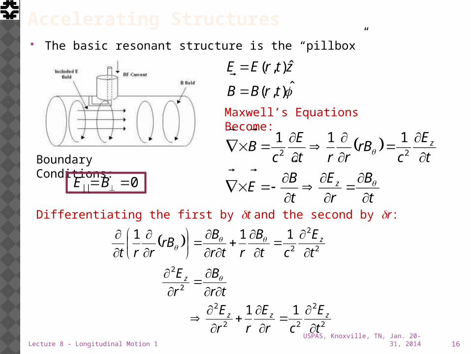
Accelerating Structures The basic resonant structure is the “pillbox”


),(

ˆ),(

trBB

ztrEE

t

B

r

E

t

BE

t

E

crB

rrt

E

cB

z

z

22

111

Maxwell’s Equations Become:

Differentiating the first by dt and the second by dr:

2

2

22

2

2

2

2

2

2

11

111

t

E

cr

E

rr

E

tr

B

r

E

t

E

ct

B

rtr

BrB

rrt

zzz

z

z

Boundary Conditions:

0|| BE

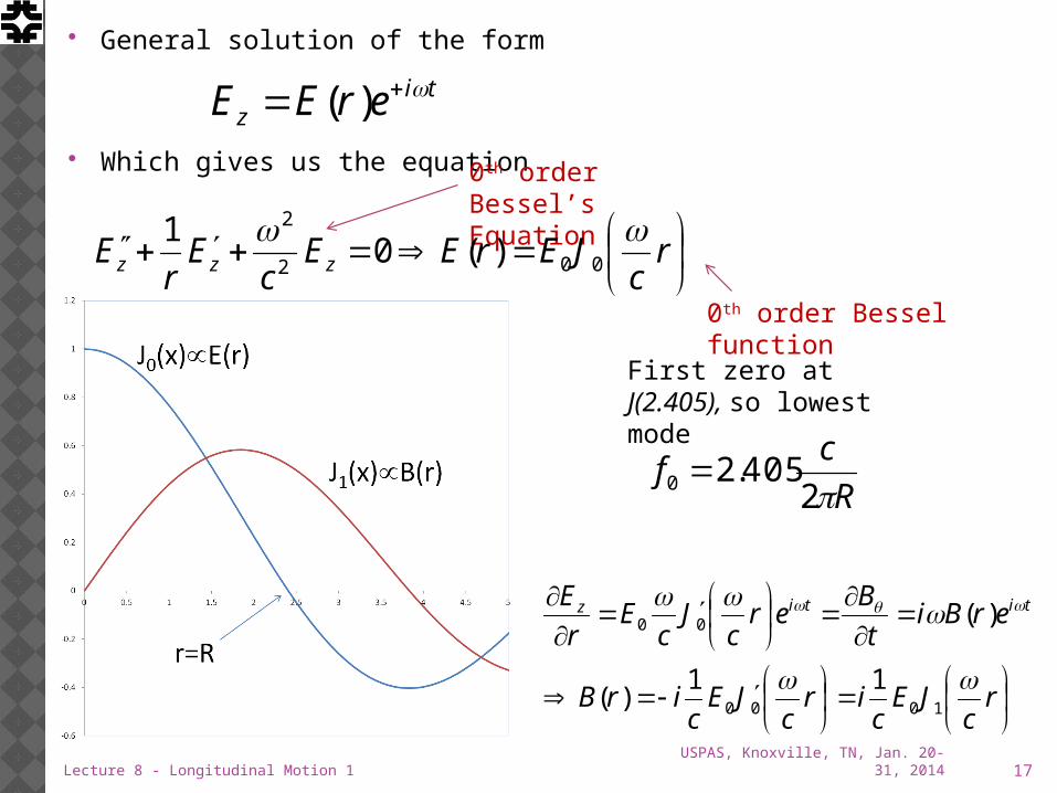
General solution of the form

Which gives us the equation


tiz erEE )(

r

cJErEE

cE

rE zzz

002

2

)(01

0th order Bessel’s Equation

0th order Bessel function

First zero at J(2.405), so lowest mode

R

cf

2405.20

rc

JEc

irc

JEc

irB

erBit

Ber

cJ

cE

r

E titiz

1000

00

11)(

)(

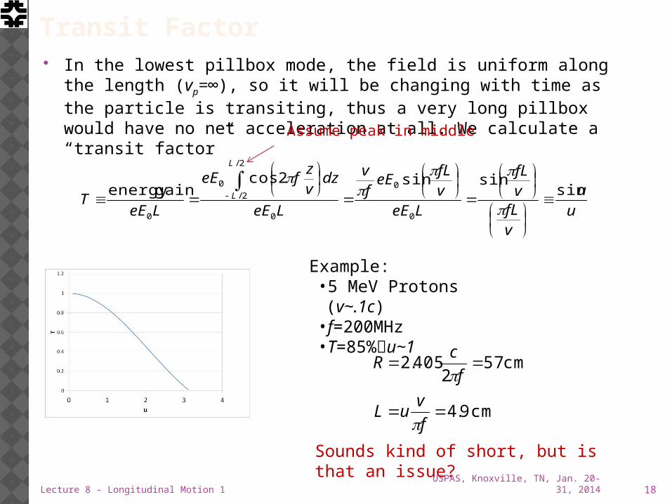
Transit Factor In the lowest pillbox mode, the field is uniform along the length

(vp=∞), so it will be changing with time as the particle is transiting, thus a very long pillbox would have no net acceleration at all. We calculate a “transit factor”


u

u

vfL

vfL

LeEvfL

eEfv

LeE

dzvz

feE

LeET

L

L sinsinsin2cos

gainenergy

0

0

0

2/

2/

0

0

Assume peak in middle

Example:• 5 MeV Protons (v~.1c)• f=200MHz• T=85%u~1

cm 9.4

cm 57 2

405.2

f

vuL

f

cR

Sounds kind of short, but is that an issue?

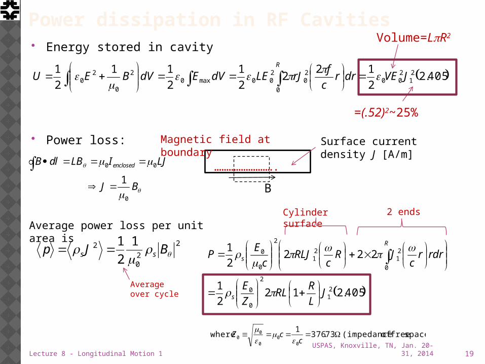
Power dissipation in RF Cavities Energy stored in cavity

Power loss:


405.22

122

2

1

2

11

2

1 21

200

0

20

200max0

2

0

20 JVEdrr

c

frJLEdVEdVBEU

R

εεε

ε

=(.52)2~25%

Volume=LpR2

B

…………………….

Magnetic field at boundary

Surface current density J [A/m]

BJ

LJILBldB enclosed

0

00

1

Average power loss per unit area is

2

20

2 1

2

1

BJp ss

Average over cycle 405.212

2

1

2222

1

21

2

0

0

0

21

21

2

0

0

JL

RRL

Z

E

rdrrc

JRc

RLJc

EP

s

R

s

Cylinder surface

2 ends

space) free of (impedance 73.3761

where0

00

00

ccZε

ε

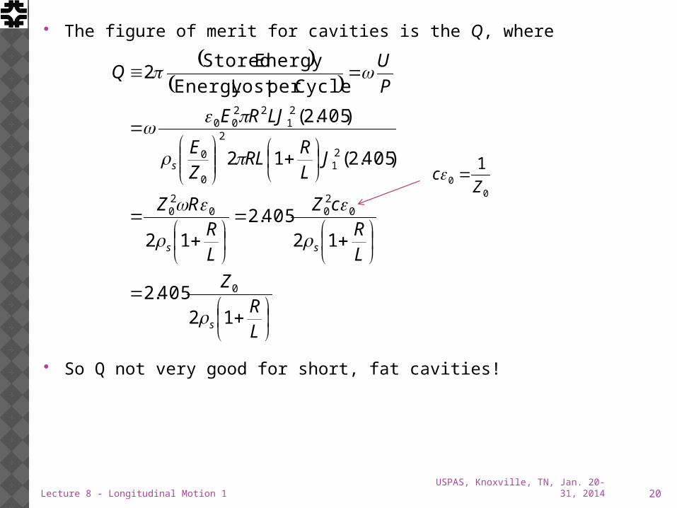
The figure of merit for cavities is the Q, where

So Q not very good for short, fat cavities!


LR

Z

LR

cZ

LR

RZ

JLR

RLZE

LJRE

P

UQ

s

ss

s

12405.2

12405.2

12

)405.2(12

)405.2(

Cycleper Lost Energy

Energy Stored2

0

0200

20

21

2

0

0

21

2200

ε

ε

ε

00

1

Zc ε

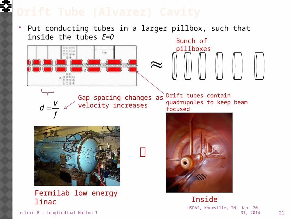
Drift Tube (Alvarez) Cavity Put conducting tubes in a larger pillbox, such that inside the tubes

E=0


Bunch of pillboxes

f

vd

Gap spacing changes as velocity increases

Drift tubes contain quadrupoles to keep beam focused

Fermilab low energy linac Inside

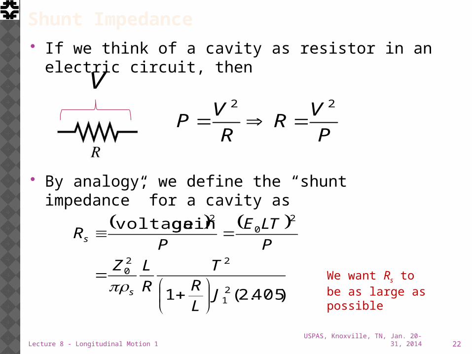
Shunt Impedance If we think of a cavity as resistor in an electric

circuit, then

By analogy, we define the “shunt impedance” for a cavity as


V

P

VR

R

VP

22

)405.2(1

gain voltage

21

220

20

2

JLR

T

R

LZ

P

LTE

PR

s

s

We want Rs to be as large as possible

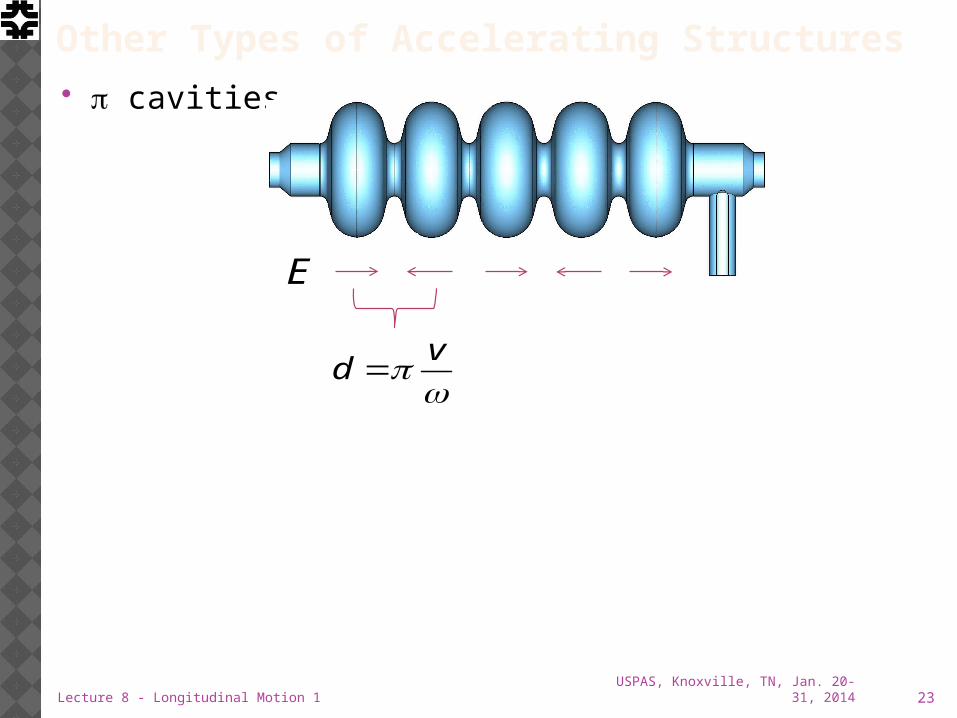
Other Types of Accelerating Structures p cavities


E

v

d

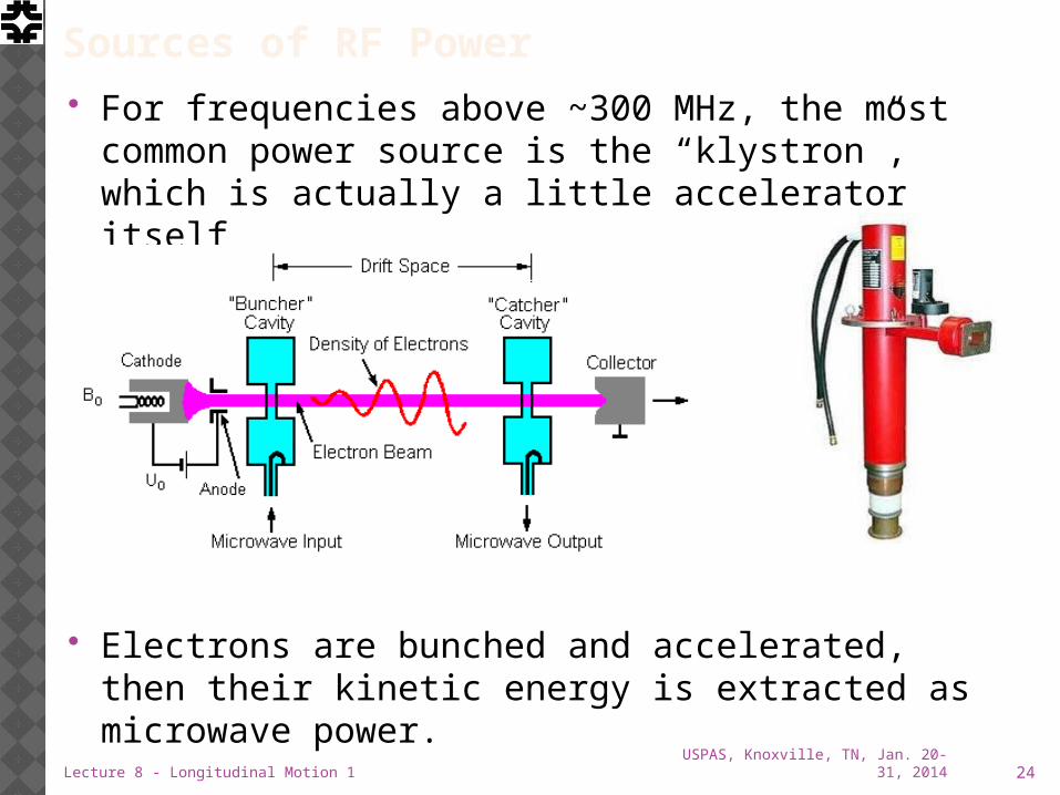
Sources of RF Power For frequencies above ~300 MHz, the most

common power source is the “klystron”, which is actually a little accelerator itself

Electrons are bunched and accelerated, then their kinetic energy is extracted as microwave power.


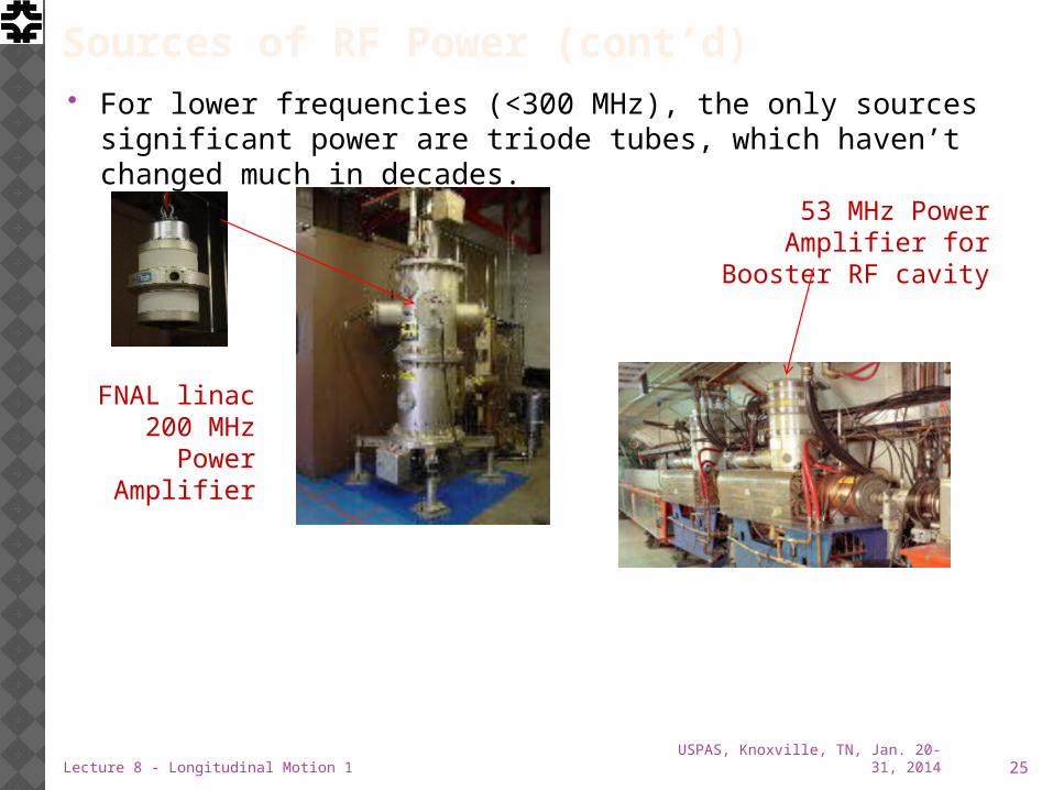
Sources of RF Power (cont’d) For lower frequencies (<300 MHz), the only sources

significant power are triode tubes, which haven’t changed much in decades.


FNAL linac 200 MHz

Power Amplifier

53 MHz Power Amplifier for Booster

RF cavity

Eric Prebys, FNAL. We consider motion of particles either through a linear structure or in a...

Documents

Transcript of Eric Prebys, FNAL. We consider motion of particles either through a linear structure or in a...