EEN320 - Power Systems I (µ ) - Part 5: The transmission line
63
EEN320 - Power Systems I (Συστήmατα Ισχύος Ι) Part 5: The transmission line Dr Petros Aristidou Department of Electrical Engineering, Computer Engineering & Informatics Last updated: March 21, 2020
Transcript of EEN320 - Power Systems I (µ ) - Part 5: The transmission line
EEN320 - Power Systems I (Συστήματα Ισχύος Ι)Part 5: The transmission line
Dr Petros AristidouDepartment of Electrical Engineering, Computer Engineering & InformaticsLast updated: March 21, 2020
Today’s learning objectives
After this part of the lecture and additional reading, you should be able to . . .1 . . . name the main components of an overhead line and describe their
functionality;
2 . . . understand how to derive the Π-equivalent circuit of a transmissionline;
3 . . . determine the parameters of the Π-equivalent circuit of a transmissionline from its concentrated parameters;
4 . . . explain how and under which conditions or assumptions theΠ-equivalent circuit can be further simplified.
,ΕΕΝ320 — Dr Petros Aristidou — Last updated: March 21, 2020 2/ 68
Outline
1 Physical relevance of power lines
2 Structure of overhead linesConductorsSupport structuresInsulatorsShield wires
3 Derivation of lumped inductor and capacitor valuesInductanceCapacitance
4 Overhead line parametersConcentrated parametersSome brief remarks on cables
5 Equivalent circuits for power linesDifferential equation of a power lineSolution of differential equation of a power lineΠ-equivalent circuitModel simplifications and their validity
,ΕΕΝ320 — Dr Petros Aristidou — Last updated: March 21, 2020 3/ 68
1 Power lines - Overview
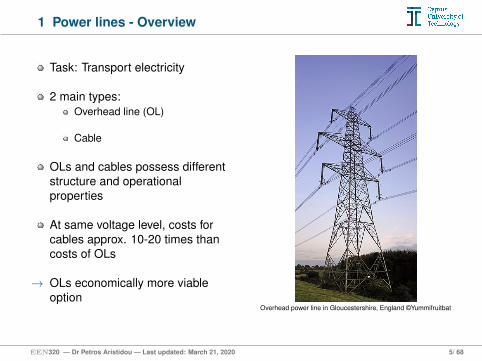
Task: Transport electricity
2 main types:Overhead line (OL)
Cable
OLs and cables possess differentstructure and operationalproperties
At same voltage level, costs forcables approx. 10-20 times thancosts of OLs
→ OLs economically more viableoption
Overhead power line in Gloucestershire, England ©Yummifruitbat
,ΕΕΝ320 — Dr Petros Aristidou — Last updated: March 21, 2020 5/ 68
1 Recap: Motivation for high voltage transmission (1)
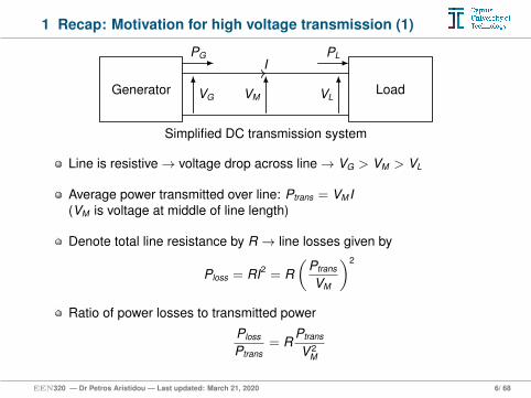
Generator Load
I
VG VM VL
PG PL
Simplified DC transmission system
Line is resistive→ voltage drop across line→ VG > VM > VL
Average power transmitted over line: Ptrans = VM I(VM is voltage at middle of line length)
Denote total line resistance by R → line losses given by
Ploss = RI2 = R(
Ptrans
VM
)2
Ratio of power losses to transmitted power
Ploss
Ptrans= R
Ptrans
V 2M
,ΕΕΝ320 — Dr Petros Aristidou — Last updated: March 21, 2020 6/ 68
1 Recap: Motivation for high voltage transmission (2)
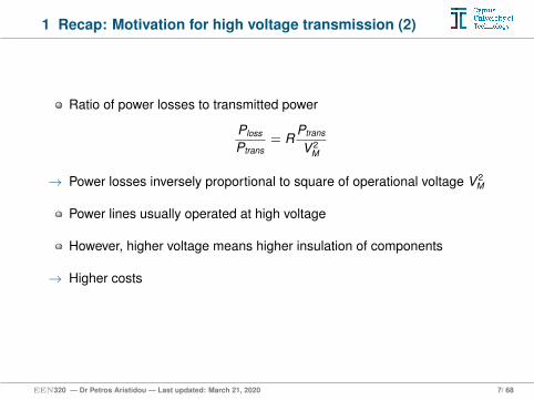
Ratio of power losses to transmitted power
Ploss
Ptrans= R
Ptrans
V 2M
→ Power losses inversely proportional to square of operational voltage V 2M
Power lines usually operated at high voltage
However, higher voltage means higher insulation of components
→ Higher costs
,ΕΕΝ320 — Dr Petros Aristidou — Last updated: March 21, 2020 7/ 68
1 Costs vs. transmission voltage
Cost
—V—
Ctot
Cmin
Vopt
ClossCinv
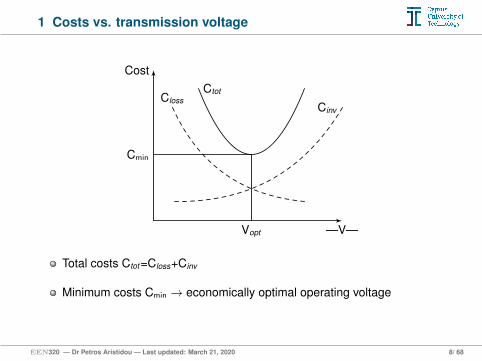
Total costs Ctot=Closs+Cinv
Minimum costs Cmin → economically optimal operating voltage
,ΕΕΝ320 — Dr Petros Aristidou — Last updated: March 21, 2020 8/ 68
2 Structure of overhead lines - Main components
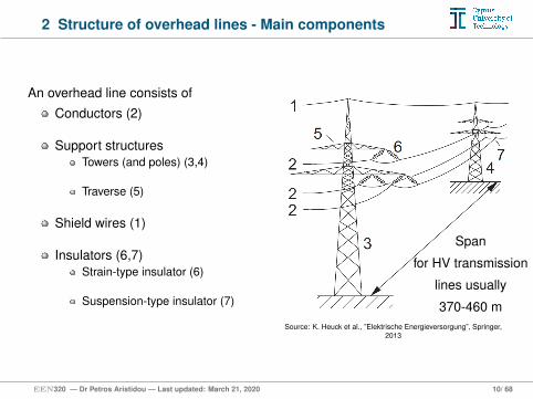
An overhead line consists of
Conductors (2)
Support structuresTowers (and poles) (3,4)
Traverse (5)
Shield wires (1)
Insulators (6,7)Strain-type insulator (6)
Suspension-type insulator (7)
Span
for HV transmission
lines usually
370-460 mSource: K. Heuck et al., ”Elektrische Energieversorgung”, Springer,
2013
,ΕΕΝ320 — Dr Petros Aristidou — Last updated: March 21, 2020 10/ 68
2.1 Conductors - Overview
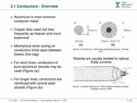
Aluminium is most commonconductor metal
Copper also used, but lessfrequently as heavier and moreexpensive
Mechanical strain acting onconductors limits span betweentowers (line sag)
For short lines, conductors ofpure aluminium strands may beused (Figure (a))
For longer lines, conductors arereinforced with central steelstrands (Figure (b))
(a) (b)Source: K. Heuck et al., ”Elektrische Energieversorgung”, Springer,
2013
Strands are usually twisted to reduceEddy currents
Source: J. Duncan Glover et al., ”Power System Analysis & Design”,Cengage Learning, 2008
,ΕΕΝ320 — Dr Petros Aristidou — Last updated: March 21, 2020 11/ 68
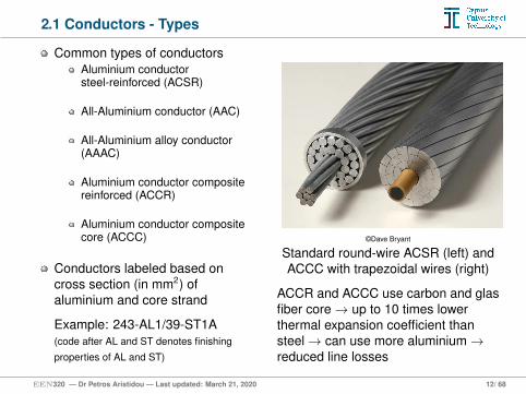
2.1 Conductors - Types
Common types of conductorsAluminium conductorsteel-reinforced (ACSR)
All-Aluminium conductor (AAC)
All-Aluminium alloy conductor(AAAC)
Aluminium conductor compositereinforced (ACCR)
Aluminium conductor compositecore (ACCC)
Conductors labeled based oncross section (in mm2) ofaluminium and core strand
Example: 243-AL1/39-ST1A(code after AL and ST denotes finishing
properties of AL and ST)
©Dave Bryant
Standard round-wire ACSR (left) andACCC with trapezoidal wires (right)
ACCR and ACCC use carbon and glasfiber core→ up to 10 times lowerthermal expansion coefficient thansteel→ can use more aluminium→reduced line losses
,ΕΕΝ320 — Dr Petros Aristidou — Last updated: March 21, 2020 12/ 68
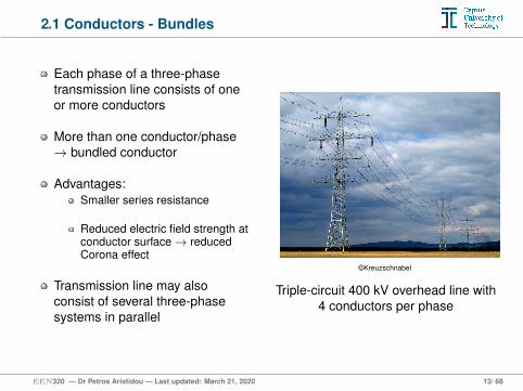
2.1 Conductors - Bundles
Each phase of a three-phasetransmission line consists of oneor more conductors
More than one conductor/phase→ bundled conductor
Advantages:Smaller series resistance
Reduced electric field strength atconductor surface→ reducedCorona effect
Transmission line may alsoconsist of several three-phasesystems in parallel
©Kreuzschnabel
Triple-circuit 400 kV overhead line with4 conductors per phase
,ΕΕΝ320 — Dr Petros Aristidou — Last updated: March 21, 2020 13/ 68
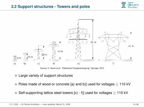
2.2 Support structures - Towers and poles
Source: K. Heuck et al., ”Elektrische Energieversorgung”, Springer, 2013
Large variety of support structures
Poles made of wood or concrete [a) and b)] used for voltages ≤ 110 kV
Self-supporting lattice steel towers [c) - f)] used for voltages ≥ 110 kV
,ΕΕΝ320 — Dr Petros Aristidou — Last updated: March 21, 2020 14/ 68
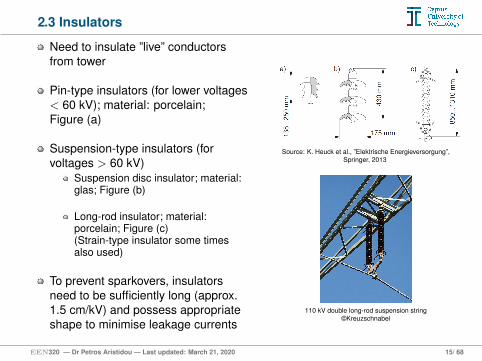
2.3 Insulators
Need to insulate ”live” conductorsfrom tower
Pin-type insulators (for lower voltages< 60 kV); material: porcelain;Figure (a)
Suspension-type insulators (forvoltages > 60 kV)
Suspension disc insulator; material:glas; Figure (b)
Long-rod insulator; material:porcelain; Figure (c)(Strain-type insulator some timesalso used)
To prevent sparkovers, insulatorsneed to be sufficiently long (approx.1.5 cm/kV) and possess appropriateshape to minimise leakage currents
Source: K. Heuck et al., ”Elektrische Energieversorgung”,Springer, 2013
110 kV double long-rod suspension string©Kreuzschnabel
,ΕΕΝ320 — Dr Petros Aristidou — Last updated: March 21, 2020 15/ 68
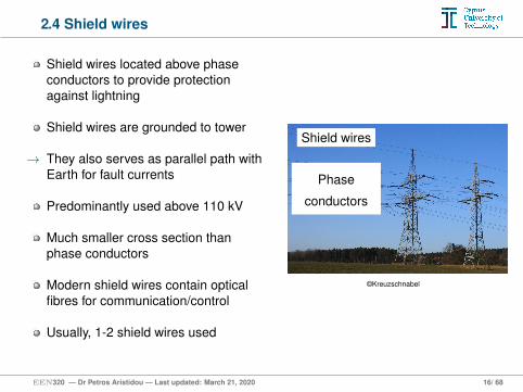
2.4 Shield wires
Shield wires located above phaseconductors to provide protectionagainst lightning
Shield wires are grounded to tower
→ They also serves as parallel path withEarth for fault currents
Predominantly used above 110 kV
Much smaller cross section thanphase conductors
Modern shield wires contain opticalfibres for communication/control
Usually, 1-2 shield wires used
Shield wires
Phase
conductors
©Kreuzschnabel
,ΕΕΝ320 — Dr Petros Aristidou — Last updated: March 21, 2020 16/ 68
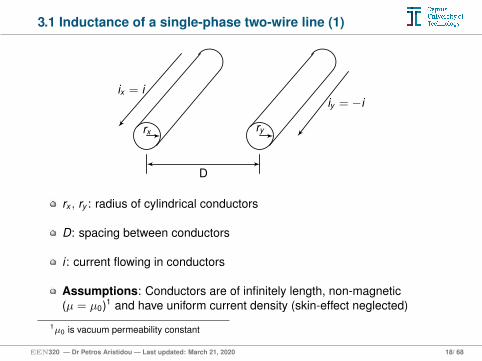
3.1 Inductance of a single-phase two-wire line (1)
rx
ix = i
ry
iy = −i
D
rx , ry : radius of cylindrical conductors
D: spacing between conductors
i : current flowing in conductors
Assumptions: Conductors are of infinitely length, non-magnetic(µ = µ0)1 and have uniform current density (skin-effect neglected)
1µ0 is vacuum permeability constant,
ΕΕΝ320 — Dr Petros Aristidou — Last updated: March 21, 2020 18/ 68
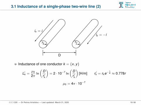
3.1 Inductance of a single-phase two-wire line (2)
rx
ix = i
ry
iy = −i
D
Inductance of one conductor k = x , y
L′k =µ0
2πln
(Dr ′k
)= 2 · 10−7 ln
(Dr ′k
)[H/m] r ′k = rk e−
14 ≈ 0.778r
µ0 = 4π · 10−7
,ΕΕΝ320 — Dr Petros Aristidou — Last updated: March 21, 2020 19/ 68
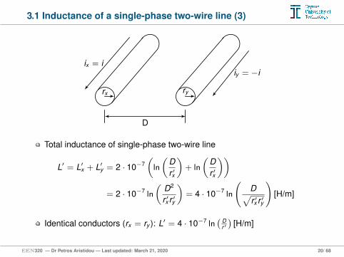
3.1 Inductance of a single-phase two-wire line (3)
rx
ix = i
ry
iy = −i
D
Total inductance of single-phase two-wire line
L′ = L′x + L′y = 2 · 10−7(
ln
(Dr ′x
)+ ln
(Dr ′x
))= 2 · 10−7 ln
(D2
r ′x r ′y
)= 4 · 10−7 ln
(D√r ′x r ′y
)[H/m]
Identical conductors (rx = ry ): L′ = 4 · 10−7 ln( D
r ′)
[H/m]
,ΕΕΝ320 — Dr Petros Aristidou — Last updated: March 21, 2020 20/ 68
3.1 Inductance of a three-phase three-wire line
a
c
b
ND D
Dr
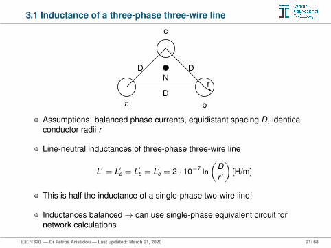
Assumptions: balanced phase currents, equidistant spacing D, identicalconductor radii r
Line-neutral inductances of three-phase three-wire line
L′ = L′a = L′b = L′c = 2 · 10−7 ln
(Dr ′
)[H/m]
This is half the inductance of a single-phase two-wire line!
Inductances balanced→ can use single-phase equivalent circuit fornetwork calculations
,ΕΕΝ320 — Dr Petros Aristidou — Last updated: March 21, 2020 21/ 68
3.1 Inductance of a three-phase three-wire line -Transposition of conductors
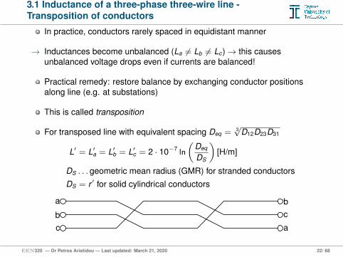
In practice, conductors rarely spaced in equidistant manner
→ Inductances become unbalanced (La 6= Lb 6= Lc)→ this causesunbalanced voltage drops even if currents are balanced!
Practical remedy: restore balance by exchanging conductor positionsalong line (e.g. at substations)
This is called transposition
For transposed line with equivalent spacing Deq = 3√
D12D23D31
L′ = L′a = L′b = L′c = 2 · 10−7 ln
(Deq
DS
)[H/m]
DS . . . geometric mean radius (GMR) for stranded conductors
DS = r ′ for solid cylindrical conductors
a
ab
b
c
c
,ΕΕΝ320 — Dr Petros Aristidou — Last updated: March 21, 2020 22/ 68
3.1 Example: Determine inductance of a three-phasethree-wire line
Task. A completely transposed 50-Hz three-phase line has flat horizontalphase spacing with 10m between adjacent conductors. The geometric meanradius (GMS) of the conductors is 0.0159m. The line length is ` = 200km.Determine the inductance in H and the inductive reactance in Ω.
Solution. (On board)
We have that
Deq =3√
10 · 10 · 20 = 12.6 m
Hence,
L′ = 2 · 10−7 ln
(Deq
DS
)= 2 · 10−7 ln
(12.6
0.0159
)= 1.335µ H/km
andL = L′ · ` = 1.335 · 10−6 · 200 = 0.267 H,
as well asX = Lω = 0.267 · 2 · π · 50 = 83.88 Ω
,ΕΕΝ320 — Dr Petros Aristidou — Last updated: March 21, 2020 23/ 68
3.2 Capacitance - Coupling and earth capacitances
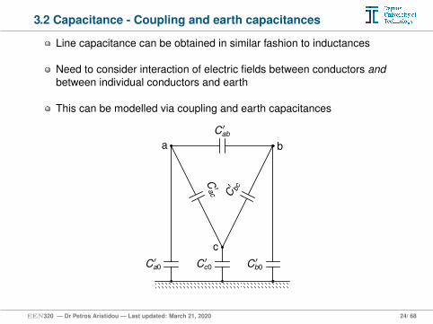
Line capacitance can be obtained in similar fashion to inductances
Need to consider interaction of electric fields between conductors andbetween individual conductors and earth
This can be modelled via coupling and earth capacitances
C′a0
a
C′c0
c
C′b0
b
C′ac
C′ab
C′ bc
,ΕΕΝ320 — Dr Petros Aristidou — Last updated: March 21, 2020 24/ 68
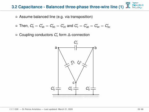
3.2 Capacitance - Balanced three-phase three-wire line (1)
Assume balanced line (e.g. via transposition)
Then, C′0 = C′a0 = C′b0 = C′c0 and C′c = C′ab = C′ac = C′bc
Coupling conductors C′c form ∆-connection
C′0
a
C′0
c
C′0
b
C′c
C′c
C′ c
,ΕΕΝ320 — Dr Petros Aristidou — Last updated: March 21, 2020 25/ 68
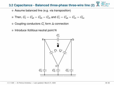
3.2 Capacitance - Balanced three-phase three-wire line (2)
Assume balanced line (e.g. via transposition)
Then, C′0 = C′a0 = C′b0 = C′c0 and C′c = C′ab = C′ac = C′bc
Coupling conductors C′c form ∆-connection
Introduce fictitious neutral point N
C′0
a
C′0
c
C′0
b
C′c
C′c
C′ c
N
,ΕΕΝ320 — Dr Petros Aristidou — Last updated: March 21, 2020 26/ 68
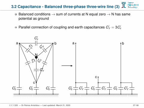
3.2 Capacitance - Balanced three-phase three-wire line (3)
Balanced conditions→ sum of currents at N equal zero→ N has samepotential as ground
Parallel connection of coupling and earth capacitances C′Y = 3C′c
C′0
a
C′0
c
C′0
b
C′c
C′cC′ c
N
C′Y
C ′Y C
′Y
C′0
a
C′0
c
C′0
b
C′Y C′Y C′Y
,ΕΕΝ320 — Dr Petros Aristidou — Last updated: March 21, 2020 27/ 68
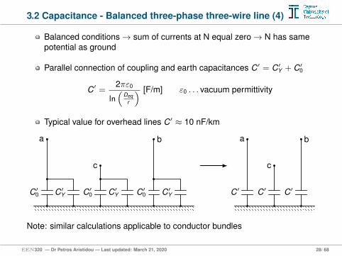
3.2 Capacitance - Balanced three-phase three-wire line (4)
Balanced conditions→ sum of currents at N equal zero→ N has samepotential as ground
Parallel connection of coupling and earth capacitances C′ = C′Y + C′0
C′ =2πε0
ln(
Deqr
) [F/m] ε0 . . . vacuum permittivity
Typical value for overhead lines C′ ≈ 10 nF/km
C′0
a
C′0
c
C′0
b
C′Y C′Y C′Y C′
a
C′
c
C′
b
Note: similar calculations applicable to conductor bundles
,ΕΕΝ320 — Dr Petros Aristidou — Last updated: March 21, 2020 28/ 68
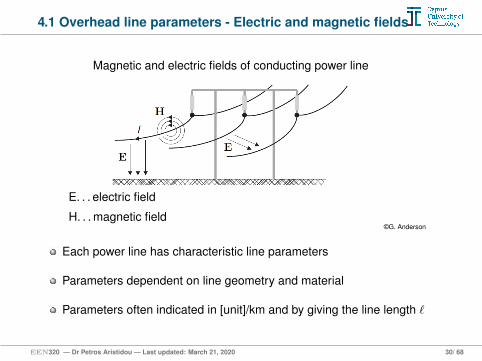
4.1 Overhead line parameters - Electric and magnetic fields
Magnetic and electric fields of conducting power line
E. . . electric field
H. . . magnetic field©G. Anderson
Each power line has characteristic line parameters
Parameters dependent on line geometry and material
Parameters often indicated in [unit]/km and by giving the line length `
,ΕΕΝ320 — Dr Petros Aristidou — Last updated: March 21, 2020 30/ 68
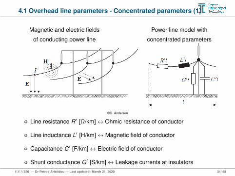
4.1 Overhead line parameters - Concentrated parameters (1)
Magnetic and electric fields
of conducting power line
Power line model with
concentrated parameters
©G. Anderson
Line resistance R′ [Ω/km]↔ Ohmic resistance of conductor
Line inductance L′ [H/km]↔ Magnetic field of conductor
Capacitance C′ [F/km]↔ Electric field of conductor
Shunt conductance G′ [S/km]↔ Leakage currents at insulators,
ΕΕΝ320 — Dr Petros Aristidou — Last updated: March 21, 2020 31/ 68
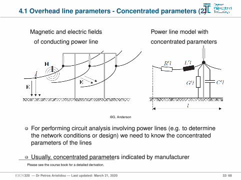
4.1 Overhead line parameters - Concentrated parameters (2)
Magnetic and electric fields
of conducting power line
Power line model with
concentrated parameters
©G. Anderson
For performing circuit analysis involving power lines (e.g. to determinethe network conditions or design) we need to know the concentratedparameters of the lines
Usually, concentrated parameters indicated by manufacturerPlease see the course book for a detailed derivation.
,ΕΕΝ320 — Dr Petros Aristidou — Last updated: March 21, 2020 32/ 68
4.1 Resistance - AC vs. DC resistance
Real conductors are not lossless!
→ This can be accounted for by including a series resistance in theconductor model
For DC current, resistance of conductor can easily be determined fromits diameter, length and specific conductivity
For AC current, in addition the skin effect needs to be considered whendetermining the resistance of a conductor
Skin-effect: current not distributed homogeneously over conductordiameter, but concentrated towards conductor boundaries
→ Current density increases towards conductor boundaries
→ Effective diameter of conductor is reduced and, hence, ohmic resistanceis increased compared to DC resistance (typically by a few percent)
,ΕΕΝ320 — Dr Petros Aristidou — Last updated: March 21, 2020 33/ 68
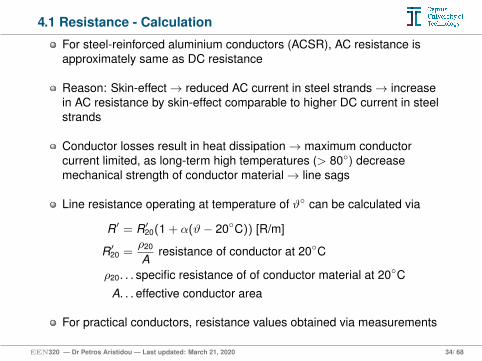
4.1 Resistance - Calculation
For steel-reinforced aluminium conductors (ACSR), AC resistance isapproximately same as DC resistance
Reason: Skin-effect→ reduced AC current in steel strands→ increasein AC resistance by skin-effect comparable to higher DC current in steelstrands
Conductor losses result in heat dissipation→ maximum conductorcurrent limited, as long-term high temperatures (> 80) decreasemechanical strength of conductor material→ line sags
Line resistance operating at temperature of ϑ can be calculated via
R′ = R′20(1 + α(ϑ− 20C)) [R/m]
R′20 =ρ20
Aresistance of conductor at 20C
ρ20. . . specific resistance of of conductor material at 20C
A. . . effective conductor area
For practical conductors, resistance values obtained via measurements
,ΕΕΝ320 — Dr Petros Aristidou — Last updated: March 21, 2020 34/ 68
4.1 Conductance
Also, losses due to insulator leakage currents and corona
Corona: high value of electric field strength at conductor surface causesair to become electrically ionised and to conduct
Corona losses dependent on meteorological conditions (rain; humidity)and conductor surface irregularities
For overhead lines, conductance G′ can only be estimated frommeasurements, while it can be determined experimentally for cables
Usually, conductance is very small and therefore most often neglected inpower system studies
,ΕΕΝ320 — Dr Petros Aristidou — Last updated: March 21, 2020 35/ 68
4.2 Cables vs. overhead lines
Cables mostly used at low voltage levels (<110 kV)
Often installed underground
Physical characteristics of cables fundamentally different from overheadtransmission lines (OHLs)!
Main reasons:Distance between conductors as well as between conductors and earthmuch smaller in cables than in OHLs
Conductors in cables typically surrounded by other metallic materials, e.g.skin
Insulation material of OHLs is air, while in cables materials such as paper, oilor SF6 are used
Consequences:Inductance of OHLs usually higher as that of cables
Capacitance of cables usually much higher as that of OHLs
,ΕΕΝ320 — Dr Petros Aristidou — Last updated: March 21, 2020 36/ 68
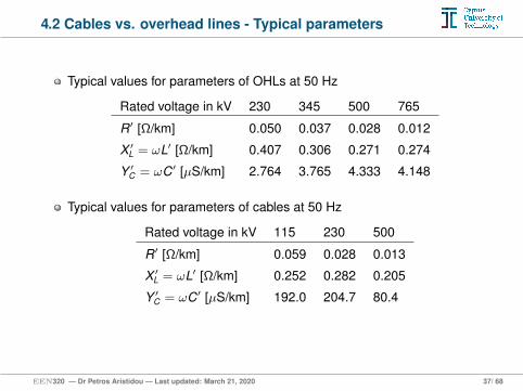
4.2 Cables vs. overhead lines - Typical parameters
Typical values for parameters of OHLs at 50 Hz
Rated voltage in kV 230 345 500 765
R′ [Ω/km] 0.050 0.037 0.028 0.012
X ′L = ωL′ [Ω/km] 0.407 0.306 0.271 0.274
Y ′C = ωC′ [µS/km] 2.764 3.765 4.333 4.148
Typical values for parameters of cables at 50 Hz
Rated voltage in kV 115 230 500
R′ [Ω/km] 0.059 0.028 0.013
X ′L = ωL′ [Ω/km] 0.252 0.282 0.205
Y ′C = ωC′ [µS/km] 192.0 204.7 80.4
,ΕΕΝ320 — Dr Petros Aristidou — Last updated: March 21, 2020 37/ 68
5 Why do we need power line models?
Being able to describe the behaviour of a power systems by amathematical model is a fundamental prerequisite for network planningand operation
We will derive a model of a power line that is valid under stationary (orsteady-state) conditions
Note: A real power system is never exactly in steady-state due tocontinuous variations of load and generation
However, under normal conditions this variations are of small magnitudecompared to overall power flows in network
Also, normal load patterns change over fairly long period (several tens ofminutes)
→ Steady-state model suitable for describing nominal network operatingconditions
,ΕΕΝ320 — Dr Petros Aristidou — Last updated: March 21, 2020 39/ 68
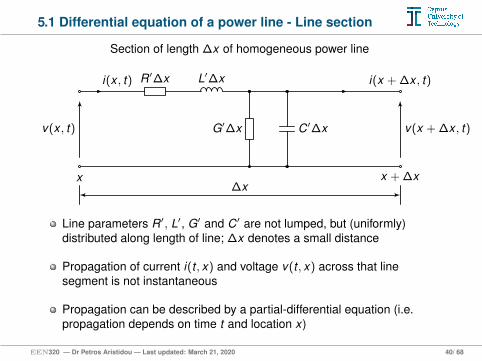
5.1 Differential equation of a power line - Line section
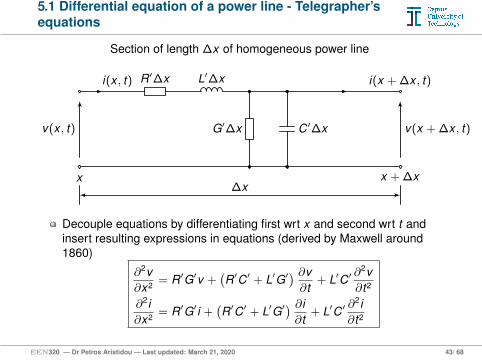
Section of length ∆x of homogeneous power line
i(x , t) R′∆x L′∆x
G′∆x
i(x + ∆x , t)
C′∆xv(x , t) v(x + ∆x , t)
∆xx x + ∆x
Line parameters R′, L′, G′ and C′ are not lumped, but (uniformly)distributed along length of line; ∆x denotes a small distance
Propagation of current i(t , x) and voltage v(t , x) across that linesegment is not instantaneous
Propagation can be described by a partial-differential equation (i.e.propagation depends on time t and location x)
,ΕΕΝ320 — Dr Petros Aristidou — Last updated: March 21, 2020 40/ 68
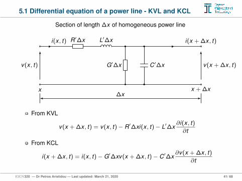
5.1 Differential equation of a power line - KVL and KCL
Section of length ∆x of homogeneous power line
i(x , t) R′∆x L′∆x
G′∆x
i(x + ∆x , t)
C′∆xv(x , t) v(x + ∆x , t)
∆xx x + ∆x
From KVL
v(x + ∆x , t) = v(x , t)− R′∆xi(x , t)− L′∆x∂i(x , t)∂t
From KCL
i(x + ∆x , t) = i(x , t)−G′∆xv(x + ∆x , t)− C′∆x∂v(x + ∆x , t)
∂t
,ΕΕΝ320 — Dr Petros Aristidou — Last updated: March 21, 2020 41/ 68
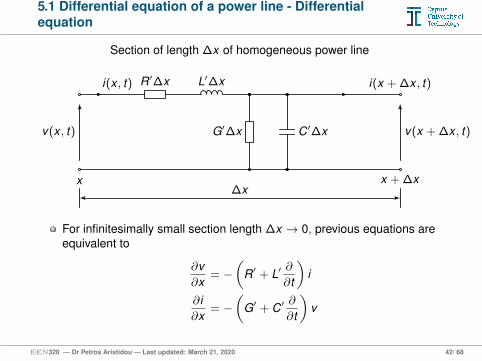
5.1 Differential equation of a power line - Differentialequation
Section of length ∆x of homogeneous power line
i(x , t) R′∆x L′∆x
G′∆x
i(x + ∆x , t)
C′∆xv(x , t) v(x + ∆x , t)
∆xx x + ∆x
For infinitesimally small section length ∆x → 0, previous equations areequivalent to
∂v∂x
= −(
R′ + L′∂
∂t
)i
∂i∂x
= −(
G′ + C′∂
∂t
)v
,ΕΕΝ320 — Dr Petros Aristidou — Last updated: March 21, 2020 42/ 68
5.1 Differential equation of a power line - Telegrapher’sequations
Section of length ∆x of homogeneous power line
i(x , t) R′∆x L′∆x
G′∆x
i(x + ∆x , t)
C′∆xv(x , t) v(x + ∆x , t)
∆xx x + ∆x
Decouple equations by differentiating first wrt x and second wrt t andinsert resulting expressions in equations (derived by Maxwell around1860)
∂2v∂x2 = R′G′v +
(R′C′ + L′G′
) ∂v∂t
+ L′C′∂2v∂t2
∂2i∂x2 = R′G′i +
(R′C′ + L′G′
) ∂i∂t
+ L′C′∂2i∂t2
,ΕΕΝ320 — Dr Petros Aristidou — Last updated: March 21, 2020 43/ 68
5.2 Introducing phasors to solve telegrapher’s equations
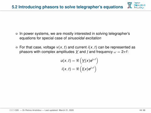
In power systems, we are mostly interested in solving telegrapher’sequations for special case of sinusoidal excitation
For that case, voltage v(x , t) and current i(x , t) can be represented asphasors with complex amplitudes V and I and frequency ω = 2πf :
u(x , t) = <(
V (x)ejωt)
i(x , t) = <(
I(x)ejωt)
,ΕΕΝ320 — Dr Petros Aristidou — Last updated: March 21, 2020 44/ 68
5.2 The wave equation
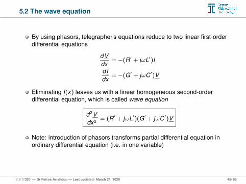
By using phasors, telegrapher’s equations reduce to two linear first-orderdifferential equations
dVdx
= −(R′ + jωL′)I
dIdx
= −(G′ + jωC′)V
Eliminating I(x) leaves us with a linear homogeneous second-orderdifferential equation, which is called wave equation
d2Vdx2 = (R′ + jωL′)(G′ + jωC′)V
Note: introduction of phasors transforms partial differential equation inordinary differential equation (i.e. in one variable)
,ΕΕΝ320 — Dr Petros Aristidou — Last updated: March 21, 2020 45/ 68
5.2 Solution of the wave equation - Voltage
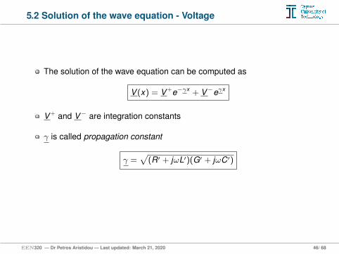
The solution of the wave equation can be computed as
V (x) = V +e−γx + V−eγx
V + and V− are integration constants
γ is called propagation constant
γ =√
(R′ + jωL′)(G′ + jωC′)
,ΕΕΝ320 — Dr Petros Aristidou — Last updated: March 21, 2020 46/ 68
5.2 Solution of the wave equation - Interpretation
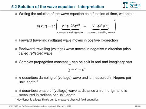
Writing the solution of the wave equation as a function of time, we obtain
v(x , t) = <
V +e−γx ejωt︸ ︷︷ ︸forward travelling wave
+ V−eγx ejωt︸ ︷︷ ︸backward travelling wave
Forward travelling (voltage) wave moves in positive x-direction
Backward travelling (voltage) wave moves in negative x-direction (alsocalled reflected wave)
Complex propagation constant γ can be split in real and imaginary part
γ = α + jβ
α describes damping of (voltage) wave and is measured in Nepers perunit length 2
β describes phase of (voltage) wave at distance x from origin and ismeasured in radians per unit length
2Np=Neper is a logarithmic unit to measure physical field quantities.,
ΕΕΝ320 — Dr Petros Aristidou — Last updated: March 21, 2020 47/ 68
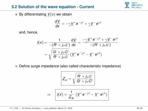
5.2 Solution of the wave equation - Current
By differentiating V (x) we obtain
dVdx
= −γV +e−γx + γV−eγx
and, hence,
I(x) =1
−(R′ + jωL′)dVdx
=−γV +e−γx + γV−eγx
−(R′ + jωL′)
=
√G′ + jωC′
R′ + jωL′(V +e−γx − V−eγx)
Define surge impedance (also called characteristic impedance)
Z w =
√R′ + jωL′
G′ + jωC′
⇒ I(x) =1
Z W
(V +e−γx − V−eγx)
,ΕΕΝ320 — Dr Petros Aristidou — Last updated: March 21, 2020 48/ 68
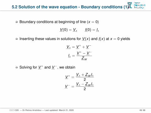
5.2 Solution of the wave equation - Boundary conditions (1)
Boundary conditions at beginning of line (x = 0)
V (0) = V 1 I(0) = I1
Inserting these values in solutions for V (x) and I(x) at x = 0 yields
V 1 = V + + V−
I1 =V + − V−
Z W
Solving for V + and V−, we obtain
V + =V 1 + Z W I1
2
V− =V 1 − Z W I1
2
,ΕΕΝ320 — Dr Petros Aristidou — Last updated: March 21, 2020 49/ 68
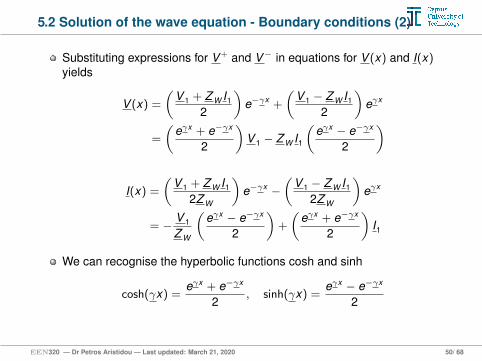
5.2 Solution of the wave equation - Boundary conditions (2)
Substituting expressions for V + and V− in equations for V (x) and I(x)yields
V (x) =
(V 1 + Z W I1
2
)e−γx +
(V 1 − Z W I1
2
)eγx
=
(eγx + e−γx
2
)V 1 − Z W I1
(eγx − e−γx
2
)
I(x) =
(V 1 + Z W I1
2Z W
)e−γx −
(V 1 − Z W I1
2Z W
)eγx
= − V 1
Z W
(eγx − e−γx
2
)+
(eγx + e−γx
2
)I1
We can recognise the hyperbolic functions cosh and sinh
cosh(γx) =eγx + e−γx
2, sinh(γx) =
eγx − e−γx
2
,ΕΕΝ320 — Dr Petros Aristidou — Last updated: March 21, 2020 50/ 68
5.2 Solution of the wave equation - Boundary conditions (3)
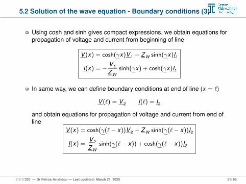
Using cosh and sinh gives compact expressions, we obtain equations forpropagation of voltage and current from beginning of line
V (x) = cosh(γx)V 1 − Z W sinh(γx)I1
I(x) = − V 1
Z Wsinh(γx) + cosh(γx)I1
In same way, we can define boundary conditions at end of line (x = `)
V (`) = V 2 I(`) = I2
and obtain equations for propagation of voltage and current from end ofline
V (x) = cosh(γ(`− x))V 2 + Z W sinh(γ(`− x))I2
I(x) =V 2
Z Wsinh(γ(`− x)) + cosh(γ(`− x))I2
,ΕΕΝ320 — Dr Petros Aristidou — Last updated: March 21, 2020 51/ 68
5.3 Simplified models of a power line
In practice, we often don’t need to use the (rather complicated) waveequation to describe phenomena in power systems
Reason: Usually, we are interested in the voltage drop across a line orthe reactive power flow, but not in the exact trajectory of the voltages andcurrents along the line
→ Then, we may use simplified models for a power line withoutcompromising the accuracy of our calculations too much
We will discuss such models in the following
In particular, we will derive the Π-equivalent circuit of a transmission line
,ΕΕΝ320 — Dr Petros Aristidou — Last updated: March 21, 2020 52/ 68
5.3 Π-equivalent circuit of homogeneous power line (1)
I1
Y q2
Z `
Y q2
I2
V 1 V 2
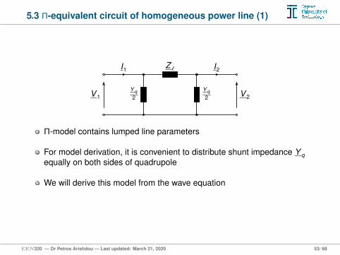
Π-model contains lumped line parameters
For model derivation, it is convenient to distribute shunt impedance Y qequally on both sides of quadrupole
We will derive this model from the wave equation
,ΕΕΝ320 — Dr Petros Aristidou — Last updated: March 21, 2020 53/ 68
5.3 Π-equivalent circuit of homogeneous power line (2)
I1
Y q2
Z `
Y q2
I2
V 1 V 2
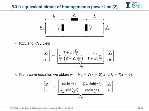
KCL and KVL yield[V 1
I1
]=
1 + Z `Y q2 Z `
Y q2
(2 + Z `
Y q2
)1 + Z `
Y q2
︸ ︷︷ ︸
=A1
[V 2
I2
]
From wave equation we obtain with V 1 = V (x = 0) and I1 = I(x = 0)[V 1
I1
]=
cosh(γ`) Z W sinh(γ`)
1Z W
sinh(γ`) cosh(γ`)
︸ ︷︷ ︸
=A2
[V 2
I2
]
,ΕΕΝ320 — Dr Petros Aristidou — Last updated: March 21, 2020 54/ 68
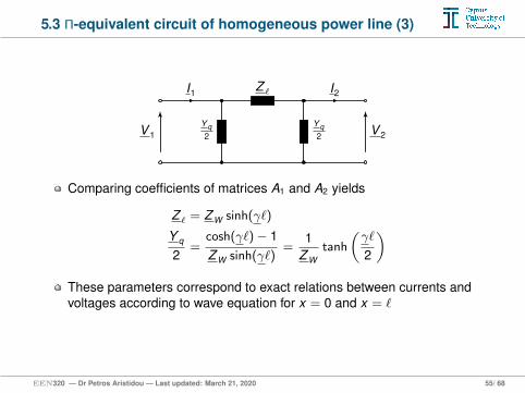
5.3 Π-equivalent circuit of homogeneous power line (3)
I1
Y q2
Z `
Y q2
I2
V 1 V 2
Comparing coefficients of matrices A1 and A2 yields
Z ` = Z W sinh(γ`)
Y q
2=
cosh(γ`)− 1Z W sinh(γ`)
=1
Z Wtanh
(γ`
2
)These parameters correspond to exact relations between currents andvoltages according to wave equation for x = 0 and x = `
,ΕΕΝ320 — Dr Petros Aristidou — Last updated: March 21, 2020 55/ 68
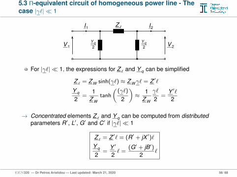
5.3 Π-equivalent circuit of homogeneous power line - Thecase |γ`| 1
I1
Y q2
Z `
Y q2
I2
V 1 V 2
For |γ`| 1, the expressions for Z ` and Y q can be simplified
Z ` = Z W sinh(γ`) ≈ Z Wγ` = Z ′`
Y q
2=
1Z W
tanh
((γ`)
2
)≈ 1
Z W
γ`
2=
Y ′`2
→ Concentrated elements Z ` and Y q can be computed from distributedparameters R′, L′, G′ and C′ if |γ`| 1
Z ` = Z ′` = (R′ + jX ′)`Y q
2=
Y ′
2` =
(G′ + jB′)2
`
,ΕΕΝ320 — Dr Petros Aristidou — Last updated: March 21, 2020 56/ 68
5.3 Π-equivalent circuit of homogeneous power line -Validity of model
Accuracy of assumption |γ`| 1 is crucial for validity of simplifiedequivalent Π-model
The larger |γ`|, the worse the model with concentrated parameters Z `and Y q represents evolution of current and voltage along the line
→ Whenever you use a simplified Π-model to represent a power line, beaware that the model accuracy reduces with increasing line length!
Rule of thumb:Max. length for overhead line ≈ 300 km
Max. length for cable ≈ 100 km
Therefore, long power lines are often split into several shorter sections inpower flow calculations and each section is represented by individual(simplified) Π-model
,ΕΕΝ320 — Dr Petros Aristidou — Last updated: March 21, 2020 57/ 68
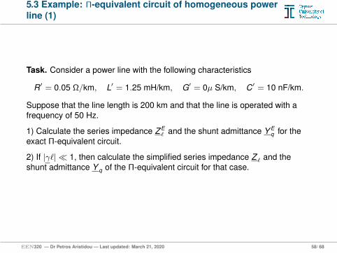
5.3 Example: Π-equivalent circuit of homogeneous powerline (1)
Task. Consider a power line with the following characteristics
R′ = 0.05 Ω/km, L′ = 1.25 mH/km, G′ = 0µ S/km, C′ = 10 nF/km.
Suppose that the line length is 200 km and that the line is operated with afrequency of 50 Hz.
1) Calculate the series impedance Z E` and the shunt admittance Y E
q for theexact Π-equivalent circuit.
2) If |γ`| 1, then calculate the simplified series impedance Z ` and theshunt admittance Y q of the Π-equivalent circuit for that case.
,ΕΕΝ320 — Dr Petros Aristidou — Last updated: March 21, 2020 58/ 68
5.3 Example: Π-equivalent circuit of homogeneous powerline (2)
Solution. (On board)
1) Surge impedance of line with G′ = 0 andω = 2πf = 314.16 rad/s
Z W =
√R′ + jωL′
jωC′
=
√0.05 + j314.16 · 1.25 · 10−3
j314.16 · 10 · 10−9 = 354.27− j22.463 = 354.98 −3.63 Ω
Propagation constant of line with G′ = 0 and ω = 2πf = 314.16rad/s
γ =√
(R′ + jωL′)(jωC′)
=√
(0.05 + j314.16 · 1.25 · 10−3)(j314.16 · 10 · 10−9)
= 0.0001 Np/km + j0.0011 [rad/km]
Np=Neper (logarithmic unit to measure physical field quantities)
,ΕΕΝ320 — Dr Petros Aristidou — Last updated: March 21, 2020 59/ 68
5.3 Example: Π-equivalent circuit of homogeneous powerline (3)
(On board)
Series impedance of Π-equivalent circuit
Z E` = Z W sinh(γ`)
= 354.98 −3.63 · sinh(0.0011 84.81 · 200)
= 11.818 + j76.889 = 77.79 81.27 Ω
Shunt admittance of Π-equivalent circuit
Y Eq =
2Z W
tanh
(γ`
2
)=
2354.98 −3.63
· tanh
(0.0011 84.81 · 200
2
)= 1.754 · 10−5 + j6.246 · 10−4 = 6.248 · 10−4 88.40 S
→ Exact Π-equivalent circuit can have shunt conductance even if3 G′ = 0!
3Physical explanation: We could model the considered line equivalently by two Π-equivalentcircuits in series. Then, we would see that there are active power losses in the circuit. Thus, thesingle Π-equivalent circuit has to have an ohmic component.
,ΕΕΝ320 — Dr Petros Aristidou — Last updated: March 21, 2020 60/ 68
5.3 Example: Π-equivalent circuit of homogeneous powerline (4)
(On board)
2) We have that
|γ`| = 0.0011 · 200 = 0.22
This value is reasonably smaller than 1
Thus, using the simplified equations valid for |γ`| 1, we obtain
Z ` = (R′ + jωL′)`
= (0.05 + j314.16 · 1.25 · 10−3) · 200
= 10 + j78.54 = 79.17 82.75 Ω
and
Y q = jB′` = jωC′`
= j314.16 · 10 · 10−9 · 200 = j6.283 · 10−4 S
→ Simplified Π-equivalent circuit has NO shunt conductance wheneverG′ = 0!
Remaining parameters are very similar to exact values:Z ` ≈ Z E
` , =(Y q) ≈ =(Y Eq )
,ΕΕΝ320 — Dr Petros Aristidou — Last updated: March 21, 2020 61/ 68
5.4 Model simplifications - (1) Lossless lines
I1
Y q2
Z `
Y q2
I2
V 1 V 2
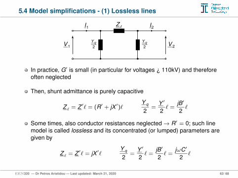
In practice, G′ is small (in particular for voltages ¿ 110kV) and thereforeoften neglected
Then, shunt admittance is purely capacitive
Z ` = Z ′` = (R′ + jX ′)`Y q
2=
Y ′
2` =
jB′
2`
Some times, also conductor resistances neglected→ R′ = 0; such linemodel is called lossless and its concentrated (or lumped) parameters aregiven by
Z ` = Z ′` = jX ′`Y q
2=
Y ′
2` =
jB′
2` =
jωC′
2`
,ΕΕΝ320 — Dr Petros Aristidou — Last updated: March 21, 2020 62/ 68
5.4 Model simplifications - (2) Medium- and short-lengthlines
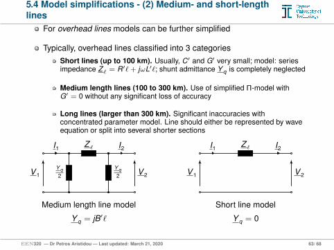
For overhead lines models can be further simplified
Typically, overhead lines classified into 3 categoriesShort lines (up to 100 km). Usually, C′ and G′ very small; model: seriesimpedance Z ` = R′` + jωL′`; shunt admittance Y q is completely neglected
Medium length lines (100 to 300 km). Use of simplified Π-model withG′ = 0 without any significant loss of accuracy
Long lines (larger than 300 km). Significant inaccuracies withconcentrated parameter model. Line should either be represented by waveequation or split into several shorter sections
I1
Y q2
Z `
Y q2
I2
Medium length line model
Y q = jB′`
V 1 V 2
I1 Z ` I2
Short line model
Y q = 0
V 1 V 2
,ΕΕΝ320 — Dr Petros Aristidou — Last updated: March 21, 2020 63/ 68
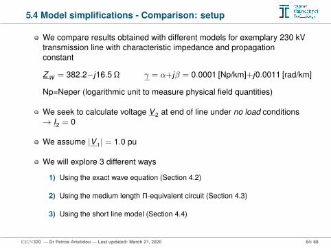
5.4 Model simplifications - Comparison: setup
We compare results obtained with different models for exemplary 230 kVtransmission line with characteristic impedance and propagationconstant
Z W = 382.2−j16.5 Ω γ = α+jβ = 0.0001 [Np/km]+j0.0011 [rad/km]
Np=Neper (logarithmic unit to measure physical field quantities)
We seek to calculate voltage V 2 at end of line under no load conditions→ I2 = 0
We assume |V 1| = 1.0 pu
We will explore 3 different ways
1) Using the exact wave equation (Section 4.2)
2) Using the medium length Π-equivalent circuit (Section 4.3)
3) Using the short line model (Section 4.4)
,ΕΕΝ320 — Dr Petros Aristidou — Last updated: March 21, 2020 64/ 68
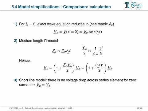
5.4 Model simplifications - Comparison: calculation
1) For I2 = 0, exact wave equation reduces to (see matrix A2)
V 1 = V (x = 0) = V 2 cosh(γ`)
2) Medium length Π-model
Z ` ≈ Z Wγ`Y q
2≈ 1
Z W
γ`
2
Hence,
V 1 =
(1 +
Z `Y q
2
)V 2 =
(1 +
(γ`)2
2
)V 2
3) Short line model: there is no voltage drop across series element for zerocurrent→ V 2 = V 1
,ΕΕΝ320 — Dr Petros Aristidou — Last updated: March 21, 2020 65/ 68
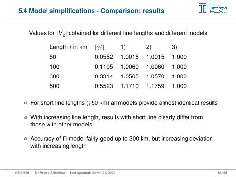
5.4 Model simplifications - Comparison: results
Values for |V 2| obtained for different line lengths and different models
Length ` in km |γ`| 1) 2) 3)
50 0.0552 1.0015 1.0015 1.000
100 0.1105 1.0060 1.0060 1.000
300 0.3314 1.0565 1.0570 1.000
500 0.5523 1.1710 1.1759 1.000
For short line lengths (¡ 50 km) all models provide almost identical results
With increasing line length, results with short line clearly differ fromthose with other models
Accuracy of Π-model fairly good up to 300 km, but increasing deviationwith increasing length
,ΕΕΝ320 — Dr Petros Aristidou — Last updated: March 21, 2020 66/ 68
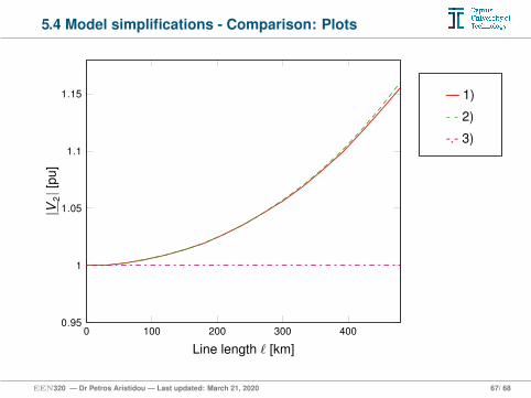
5.4 Model simplifications - Comparison: Plots
0 100 200 300 4000.95
1
1.05
1.1
1.15
Line length ` [km]
|V2|[
pu]
— 1)
- - 2)
-.- 3)
,ΕΕΝ320 — Dr Petros Aristidou — Last updated: March 21, 2020 67/ 68
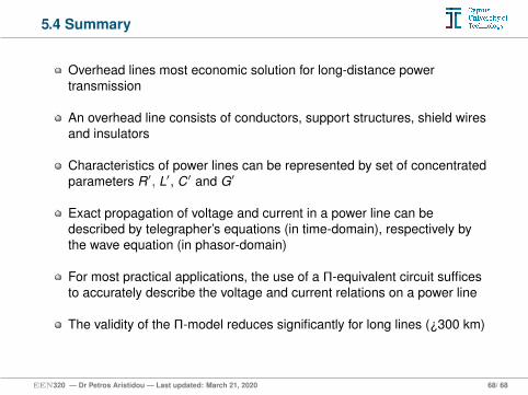
5.4 Summary
Overhead lines most economic solution for long-distance powertransmission
An overhead line consists of conductors, support structures, shield wiresand insulators
Characteristics of power lines can be represented by set of concentratedparameters R′, L′, C′ and G′
Exact propagation of voltage and current in a power line can bedescribed by telegrapher’s equations (in time-domain), respectively bythe wave equation (in phasor-domain)
For most practical applications, the use of a Π-equivalent circuit sufficesto accurately describe the voltage and current relations on a power line
The validity of the Π-model reduces significantly for long lines (¿300 km)
,ΕΕΝ320 — Dr Petros Aristidou — Last updated: March 21, 2020 68/ 68

![π °“√·ª√º‘§°“√‡√ ’¬π§≥ ‘µ»“ µ√ å —πPs].pdf · 38 ‡∑§π‘§°“√‡√ ’¬π§≥ ‘µ»“ µ√ å : °“√·ª√º —π](https://static.fdocument.org/doc/165x107/5e26221fca2e3d7e282c4145/-aoeaaaaoeaaa-aa-aaoe-a-a-pspdf.jpg)