Econometric and time series modeling using R - UFPE

Econometric and time series modeling using R

Francisco Cribari–Neto

Departamento de Estat́ısticaUniversidade Federal de Pernambuco

[email protected]

http://www.de.ufpe.br/~cribari

These slides are available at http://www.de.ufpe.br/~cribari/r_slides.pdf.

Econometric and time series analysis with R 1

“Do I use bootstrap in my own applied work? Yes, but not as much as I use the t-test, linear

regression or the standard intervals θ̂ ± 1.645σ̂. However, my bootstrapping has increasedconsiderably with the switch to S, a modern interactive computing language.

My guess is that the bootstrap (and other computer-intensive methods) will really come intoits own only as more statisticians are freed from the constraints of batch-mentality processingsystems like SAS.”

Bradley Efron, 1994


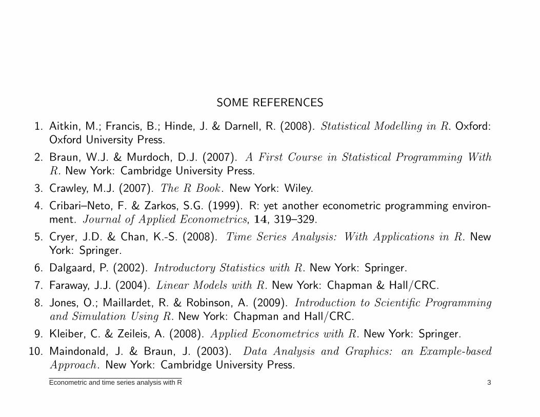
SOME REFERENCES

1. Aitkin, M.; Francis, B.; Hinde, J. & Darnell, R. (2008). Statistical Modelling in R. Oxford:Oxford University Press.

2. Braun, W.J. & Murdoch, D.J. (2007). A First Course in Statistical Programming With

R. New York: Cambridge University Press.

3. Crawley, M.J. (2007). The R Book . New York: Wiley.

4. Cribari–Neto, F. & Zarkos, S.G. (1999). R: yet another econometric programming environ-ment. Journal of Applied Econometrics, 14, 319–329.

5. Cryer, J.D. & Chan, K.-S. (2008). Time Series Analysis: With Applications in R. NewYork: Springer.

6. Dalgaard, P. (2002). Introductory Statistics with R. New York: Springer.

7. Faraway, J.J. (2004). Linear Models with R. New York: Chapman & Hall/CRC.

8. Jones, O.; Maillardet, R. & Robinson, A. (2009). Introduction to Scientific Programming

and Simulation Using R. New York: Chapman and Hall/CRC.

9. Kleiber, C. & Zeileis, A. (2008). Applied Econometrics with R. New York: Springer.

10. Maindonald, J. & Braun, J. (2003). Data Analysis and Graphics: an Example-based

Approach. New York: Cambridge University Press.


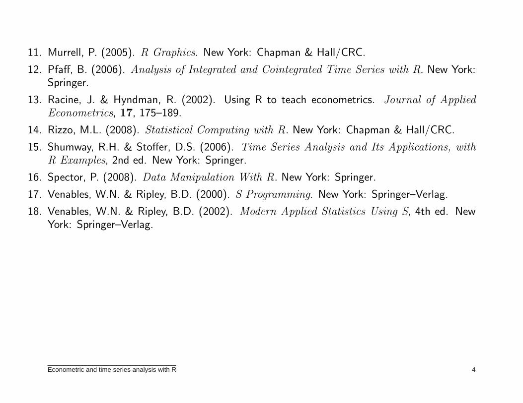
11. Murrell, P. (2005). R Graphics. New York: Chapman & Hall/CRC.

12. Pfaff, B. (2006). Analysis of Integrated and Cointegrated Time Series with R. New York:Springer.

13. Racine, J. & Hyndman, R. (2002). Using R to teach econometrics. Journal of Applied

Econometrics, 17, 175–189.

14. Rizzo, M.L. (2008). Statistical Computing with R. New York: Chapman & Hall/CRC.

15. Shumway, R.H. & Stoffer, D.S. (2006). Time Series Analysis and Its Applications, with

R Examples, 2nd ed. New York: Springer.

16. Spector, P. (2008). Data Manipulation With R. New York: Springer.

17. Venables, W.N. & Ripley, B.D. (2000). S Programming. New York: Springer–Verlag.

18. Venables, W.N. & Ripley, B.D. (2002). Modern Applied Statistics Using S, 4th ed. NewYork: Springer–Verlag.


WHAT IS R?

⊲ “S is a high-level language for manipulating and displaying data. It forms the basis of twohighly acclaimed and widely used data analysis software systems, the commercial S-PLUSand the Open Source R.” (Venables and Ripley, 2000, p.v).

⊲ “R is ‘GNU S’ - A language and environment for statistical computing and graphics. R issimilar to the award-winning S system, which was developed at Bell Laboratories by JohnChambers et al. It provides a wide variety of statistical and graphical techniques.” (The Rweb page.)

⊲ In short: (i) R is based on the S high-level programming language; (ii) R is free and opensource; (iii) R is similar in many aspected to the commercial software S-PLUS.

⊲ The R main page on the web is http://www.R-project.org, from which the binariesfor different operating systems and the documentation can be downloaded. One can alsodownload the source code of R.

⊲ There are also many additional packages available from the R web page; they can be installedin order to expand the capabilities of R in some desired directions.


⊲ R is developed by a ‘core team’ which currently consists of: Douglas Bates, John Chambers,Peter Dalgaard, Set Falcon, Robert Gentleman, Kurt Hornik, Stefano Iacus, Ross Ihaka,Friedrich Leisch, Thomas Lumley, Martin Maechler, Duncan Murdoch, Paul Murrell, Mar-tyn Plummer, Brian Ripley, Deepayan Sarkar, Duncan Temple Lang, Luke Tierney, SimonUrbanek.


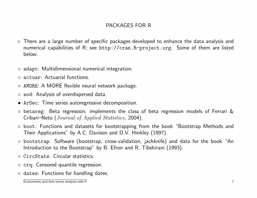
PACKAGES FOR R

⊲ There are a large number of specific packages developed to enhance the data analysis andnumerical capabilities of R; see http://cran.R-project.org. Some of them are listedbelow.

◦ adapt: Multidimensional numerical integration.

◦ actuar: Actuarial functions.

◦ AMORE: A MORE flexible neural network package.

◦ aod: Analysis of overdispersed data.

• ArDec: Time series autoregressive decomposition.

◦ betareg: Beta regression; implements the class of beta regression models of Ferrari &Cribari–Neto (Journal of Applied Statistics , 2004).

◦ boot: Functions and datasets for bootstrapping from the book “Bootstrap Methods andTheir Applications” by A.C. Davison and D.V. Hinkley (1997).

◦ bootstrap: Software (bootstrap, cross-validation, jackknife) and data for the book “AnIntroduction to the Bootstrap” by B. Efron and R. Tibshirani (1993).

◦ CircStats: Circular statistics.

◦ crq: Censored quantile regression.

◦ dates: Functions for handling dates.


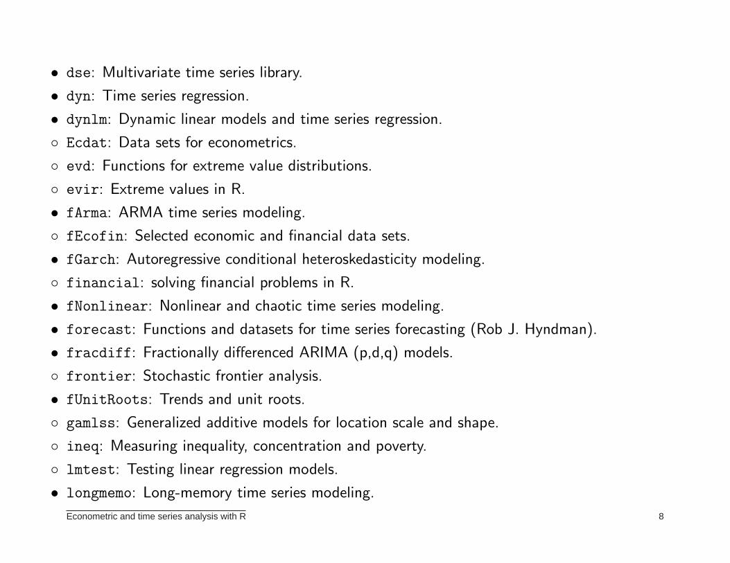
• dse: Multivariate time series library.

• dyn: Time series regression.

• dynlm: Dynamic linear models and time series regression.

◦ Ecdat: Data sets for econometrics.

◦ evd: Functions for extreme value distributions.

◦ evir: Extreme values in R.

• fArma: ARMA time series modeling.

◦ fEcofin: Selected economic and financial data sets.

• fGarch: Autoregressive conditional heteroskedasticity modeling.

◦ financial: solving financial problems in R.

• fNonlinear: Nonlinear and chaotic time series modeling.

• forecast: Functions and datasets for time series forecasting (Rob J. Hyndman).

• fracdiff: Fractionally differenced ARIMA (p,d,q) models.

◦ frontier: Stochastic frontier analysis.

• fUnitRoots: Trends and unit roots.

◦ gamlss: Generalized additive models for location scale and shape.

◦ ineq: Measuring inequality, concentration and poverty.

◦ lmtest: Testing linear regression models.

• longmemo: Long-memory time series modeling.


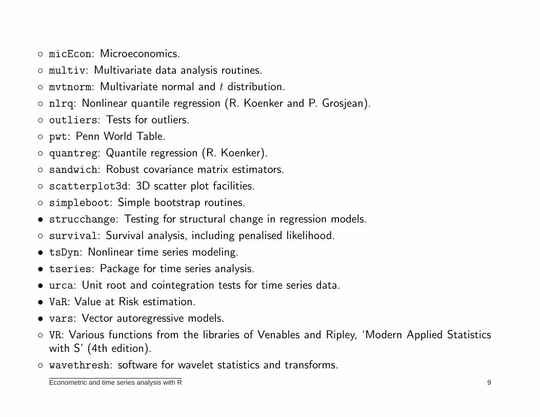
◦ micEcon: Microeconomics.

◦ multiv: Multivariate data analysis routines.

◦ mvtnorm: Multivariate normal and t distribution.

◦ nlrq: Nonlinear quantile regression (R. Koenker and P. Grosjean).

◦ outliers: Tests for outliers.

◦ pwt: Penn World Table.

◦ quantreg: Quantile regression (R. Koenker).

◦ sandwich: Robust covariance matrix estimators.

◦ scatterplot3d: 3D scatter plot facilities.

◦ simpleboot: Simple bootstrap routines.

• strucchange: Testing for structural change in regression models.

◦ survival: Survival analysis, including penalised likelihood.

• tsDyn: Nonlinear time series modeling.

• tseries: Package for time series analysis.

• urca: Unit root and cointegration tests for time series data.

• VaR: Value at Risk estimation.

• vars: Vector autoregressive models.

◦ VR: Various functions from the libraries of Venables and Ripley, ‘Modern Applied Statisticswith S’ (4th edition).

◦ wavethresh: software for wavelet statistics and transforms.


INSTALLING R PACKAGES

⊲ Example: To install the urca package:

> install.packages("urca")

⊲ To update all installed packages:

> update.packages()

Note: the computer must be connected to the Internet.

⊲ To see the list of installed packages:

> installed.packages()


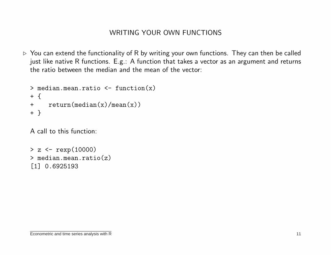
WRITING YOUR OWN FUNCTIONS

⊲ You can extend the functionality of R by writing your own functions. They can then be calledjust like native R functions. E.g.: A function that takes a vector as an argument and returnsthe ratio between the median and the mean of the vector:

> median.mean.ratio <- function(x)

+ {

+ return(median(x)/mean(x))

+ }

A call to this function:

> z <- rexp(10000)

> median.mean.ratio(z)

[1] 0.6925193


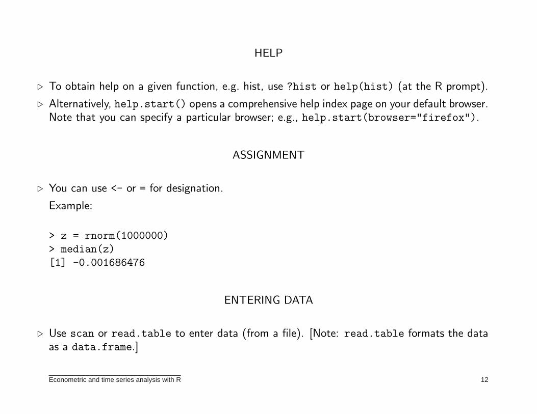
HELP

⊲ To obtain help on a given function, e.g. hist, use ?hist or help(hist) (at the R prompt).

⊲ Alternatively, help.start() opens a comprehensive help index page on your default browser.Note that you can specify a particular browser; e.g., help.start(browser="firefox").

ASSIGNMENT

⊲ You can use <- or = for designation.

Example:

> z = rnorm(1000000)

> median(z)

[1] -0.001686476

ENTERING DATA

⊲ Use scan or read.table to enter data (from a file). [Note: read.table formats the dataas a data.frame.]


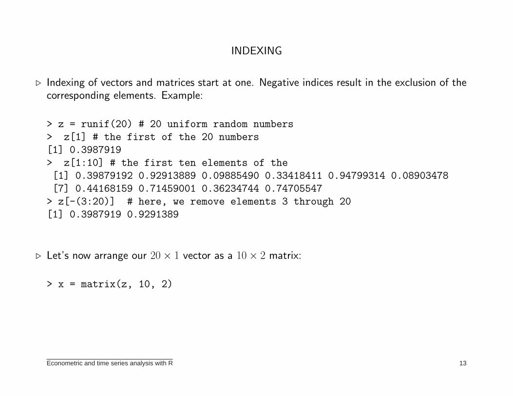
INDEXING

⊲ Indexing of vectors and matrices start at one. Negative indices result in the exclusion of thecorresponding elements. Example:

> z = runif(20) # 20 uniform random numbers

> z[1] # the first of the 20 numbers

[1] 0.3987919

> z[1:10] # the first ten elements of the

[1] 0.39879192 0.92913889 0.09885490 0.33418411 0.94799314 0.08903478

[7] 0.44168159 0.71459001 0.36234744 0.74705547

> z[-(3:20)] # here, we remove elements 3 through 20

[1] 0.3987919 0.9291389

⊲ Let’s now arrange our 20 × 1 vector as a 10 × 2 matrix:

> x = matrix(z, 10, 2)


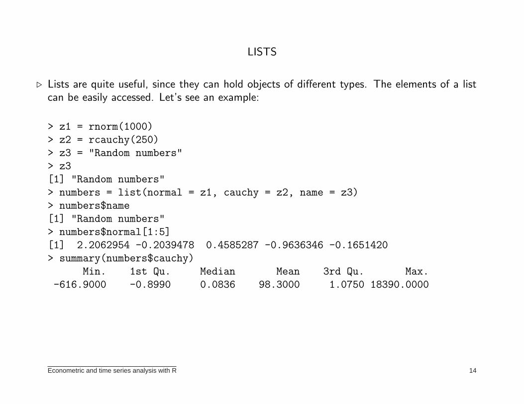
LISTS

⊲ Lists are quite useful, since they can hold objects of different types. The elements of a listcan be easily accessed. Let’s see an example:

> z1 = rnorm(1000)

> z2 = rcauchy(250)

> z3 = "Random numbers"

> z3

[1] "Random numbers"

> numbers = list(normal = z1, cauchy = z2, name = z3)

> numbers$name

[1] "Random numbers"

> numbers$normal[1:5]

[1] 2.2062954 -0.2039478 0.4585287 -0.9636346 -0.1651420

> summary(numbers$cauchy)

Min. 1st Qu. Median Mean 3rd Qu. Max.

-616.9000 -0.8990 0.0836 98.3000 1.0750 18390.0000


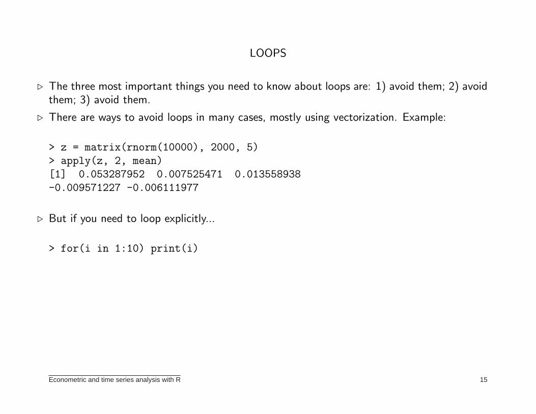
LOOPS

⊲ The three most important things you need to know about loops are: 1) avoid them; 2) avoidthem; 3) avoid them.

⊲ There are ways to avoid loops in many cases, mostly using vectorization. Example:

> z = matrix(rnorm(10000), 2000, 5)

> apply(z, 2, mean)

[1] 0.053287952 0.007525471 0.013558938

-0.009571227 -0.006111977

⊲ But if you need to loop explicitly...

> for(i in 1:10) print(i)


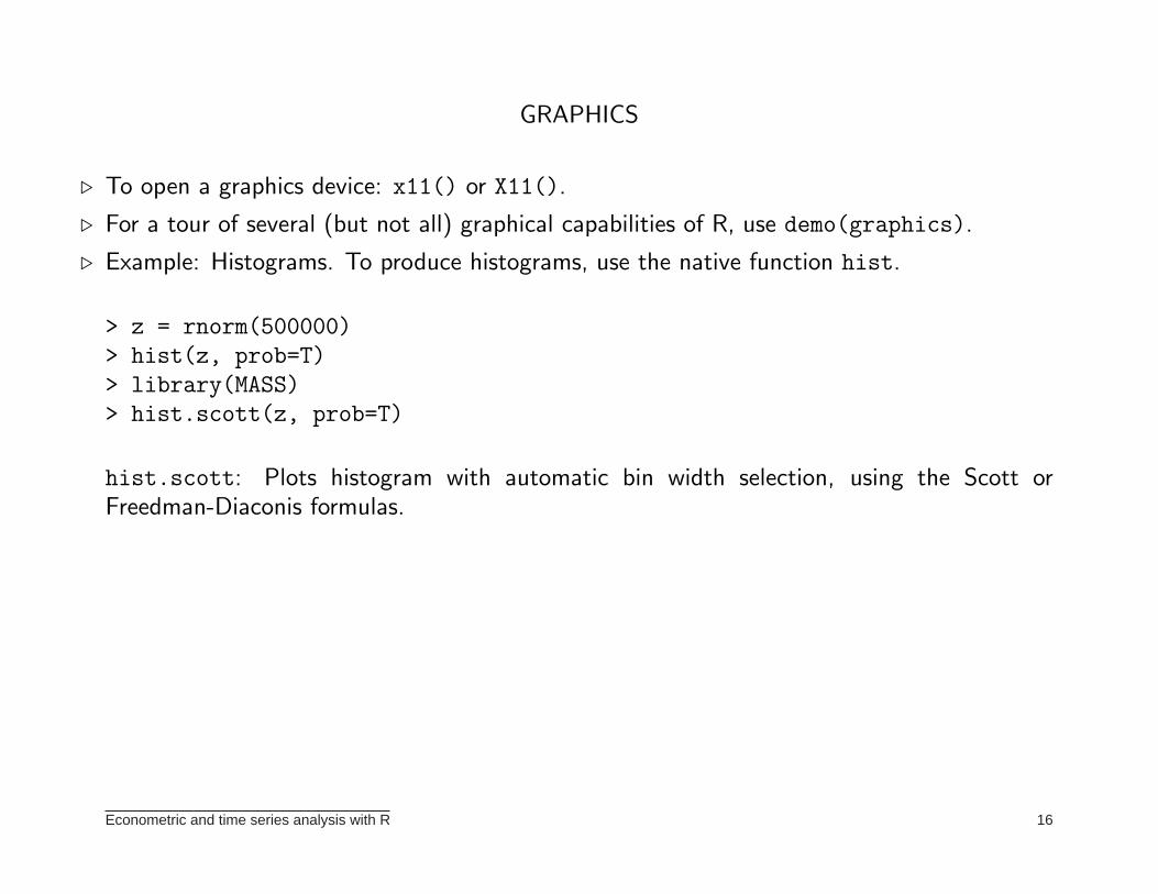
GRAPHICS

⊲ To open a graphics device: x11() or X11().

⊲ For a tour of several (but not all) graphical capabilities of R, use demo(graphics).

⊲ Example: Histograms. To produce histograms, use the native function hist.

> z = rnorm(500000)

> hist(z, prob=T)

> library(MASS)

> hist.scott(z, prob=T)

hist.scott: Plots histogram with automatic bin width selection, using the Scott orFreedman-Diaconis formulas.


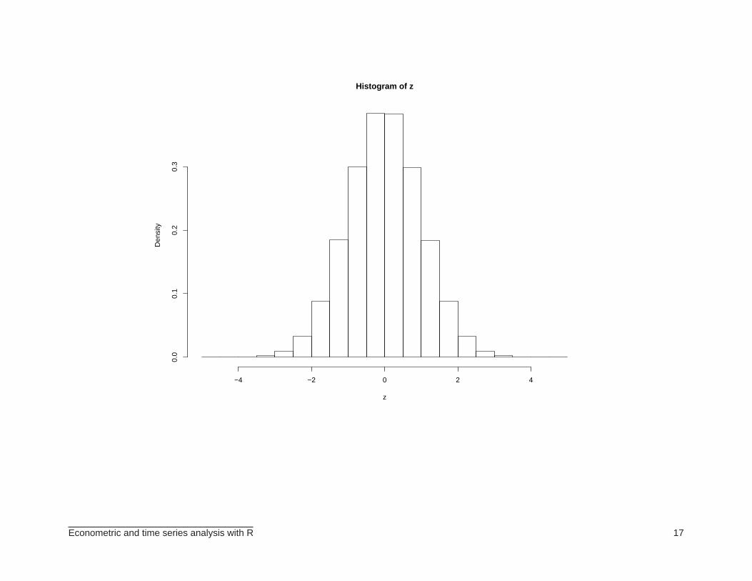
Histogram of z

z

Den

sity

−4 −2 0 2 4

0.0

0.1

0.2

0.3


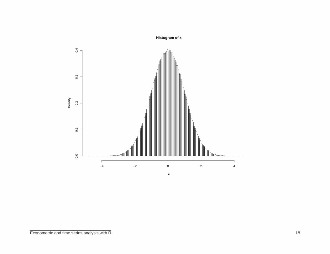
Histogram of x

z

Den

sity

−4 −2 0 2 4

0.0

0.1

0.2

0.3

0.4


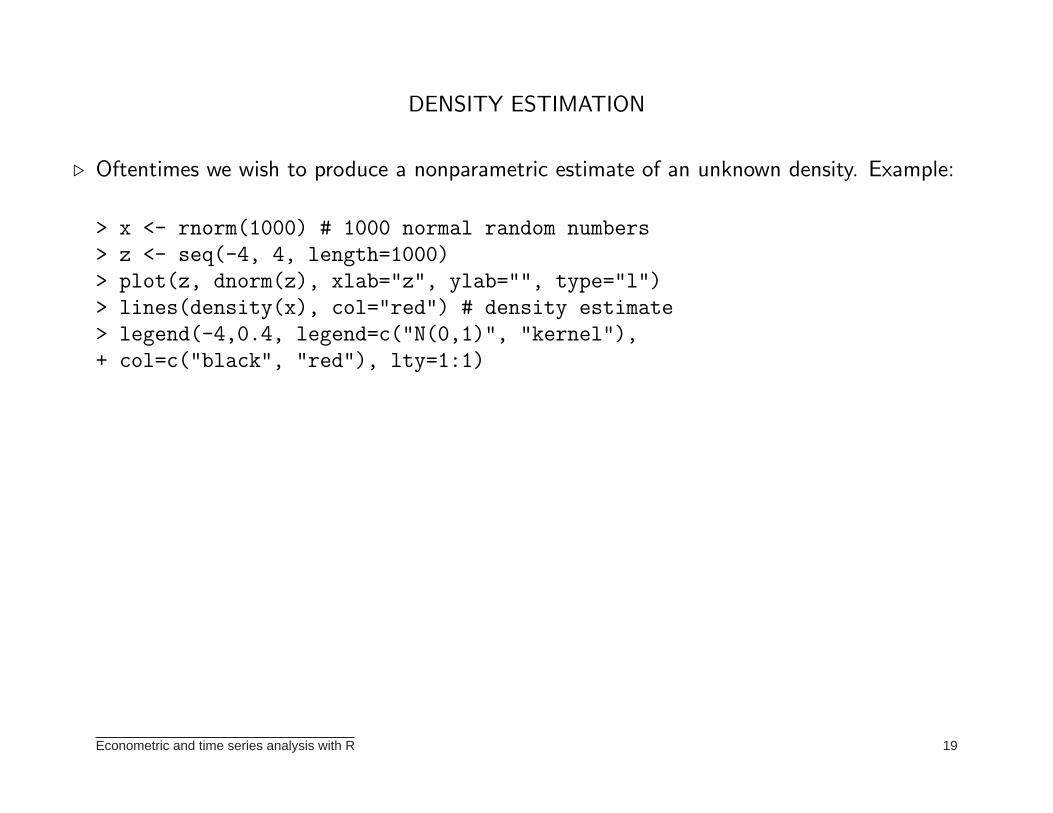
DENSITY ESTIMATION

⊲ Oftentimes we wish to produce a nonparametric estimate of an unknown density. Example:

> x <- rnorm(1000) # 1000 normal random numbers

> z <- seq(-4, 4, length=1000)

> plot(z, dnorm(z), xlab="z", ylab="", type="l")

> lines(density(x), col="red") # density estimate

> legend(-4,0.4, legend=c("N(0,1)", "kernel"),

+ col=c("black", "red"), lty=1:1)


−4 −2 0 2 4

0.0

0.1

0.2

0.3

0.4

z

N(0,1)kernel


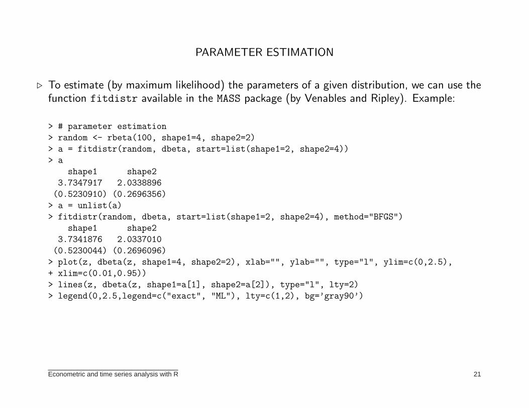
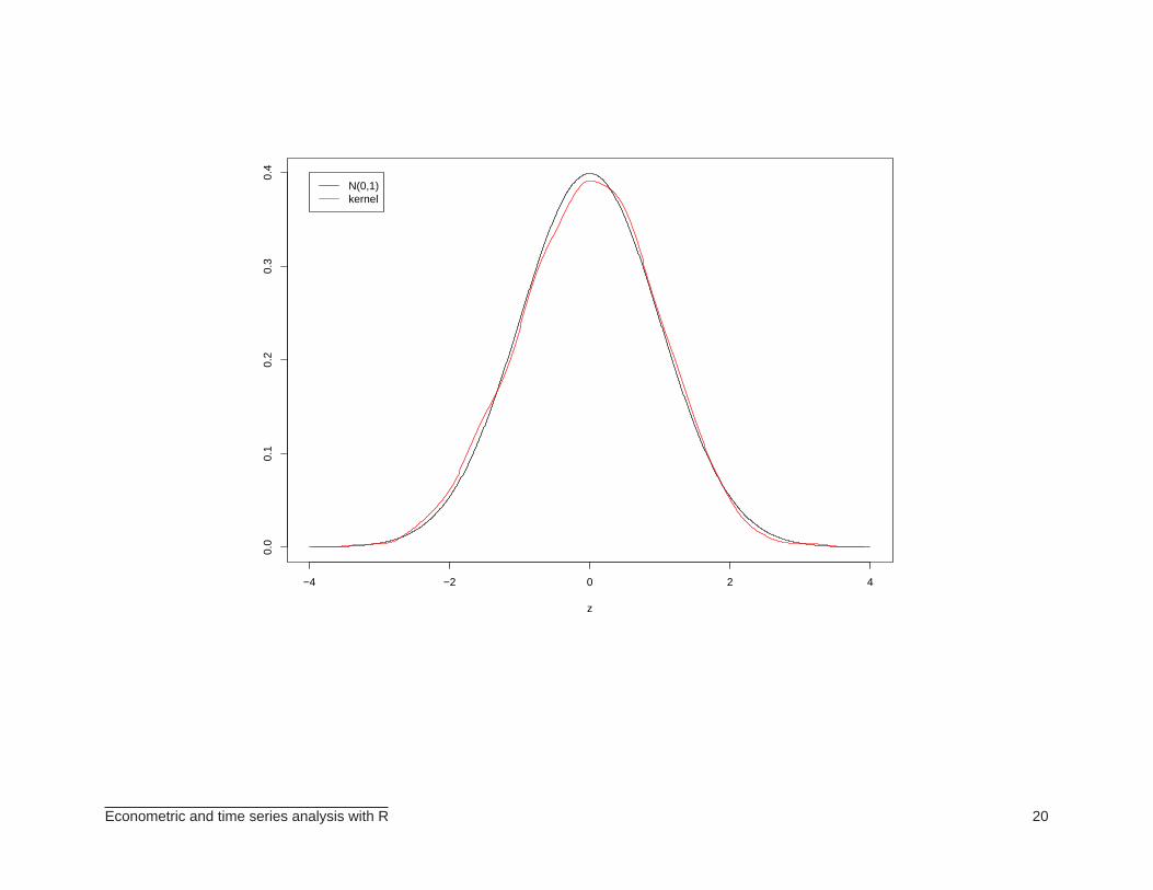
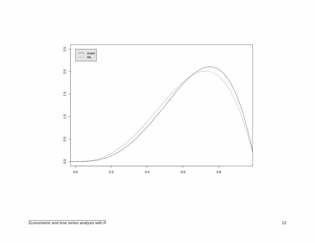
PARAMETER ESTIMATION

⊲ To estimate (by maximum likelihood) the parameters of a given distribution, we can use thefunction fitdistr available in the MASS package (by Venables and Ripley). Example:

> # parameter estimation

> random <- rbeta(100, shape1=4, shape2=2)

> a = fitdistr(random, dbeta, start=list(shape1=2, shape2=4))

> a

shape1 shape2

3.7347917 2.0338896

(0.5230910) (0.2696356)

> a = unlist(a)

> fitdistr(random, dbeta, start=list(shape1=2, shape2=4), method="BFGS")

shape1 shape2

3.7341876 2.0337010

(0.5230044) (0.2696096)

> plot(z, dbeta(z, shape1=4, shape2=2), xlab="", ylab="", type="l", ylim=c(0,2.5),

+ xlim=c(0.01,0.95))

> lines(z, dbeta(z, shape1=a[1], shape2=a[2]), type="l", lty=2)

> legend(0,2.5,legend=c("exact", "ML"), lty=c(1,2), bg=’gray90’)


0.0 0.2 0.4 0.6 0.8

0.0

0.5

1.0

1.5

2.0

2.5

exactML


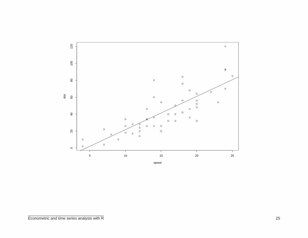
PARAMETRIC REGRESSION

⊲ Our next goal is to run a parametric regression. For linear regression, use the built-in functionlm (for linear models).

> # regression

> data(cars)

> attach(cars)

> ajuste1 <- lm(dist~speed, data=cars)

> summary(ajuste1)

Call:

lm(formula = dist ~ speed, data = cars)

Residuals:

Min 1Q Median 3Q Max

-29.069 -9.525 -2.272 9.215 43.201

Coefficients:

Estimate Std. Error t value Pr(>|t|)

(Intercept) -17.5791 6.7584 -2.601 0.0123 *

speed 3.9324 0.4155 9.464 1.49e-12 ***

---

Signif. codes: 0 ‘***’ 0.001 ‘**’ 0.01 ‘*’ 0.05

‘.’ 0.1 ‘ ’ 1


Residual standard error: 15.38 on 48 degrees of freedom

Multiple R-Squared: 0.6511, Adjusted R-squared: 0.6438

F-statistic: 89.57 on 1 and 48 DF, p-value: 1.490e-12

> plot(speed, dist)

> abline(ajuste1$coef)

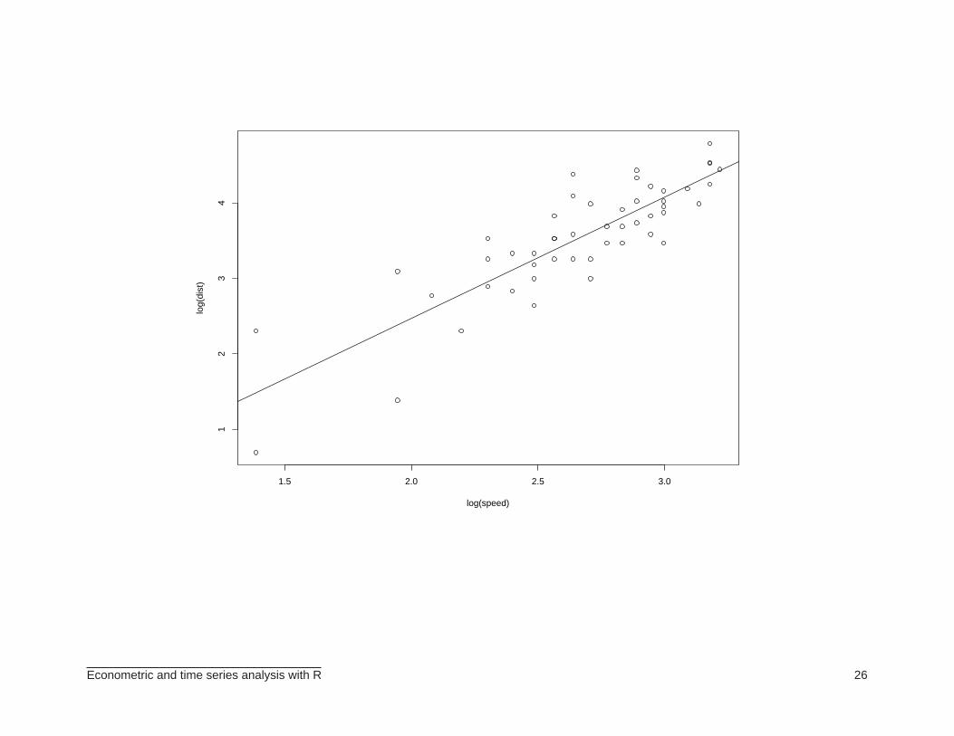
> ajuste2 <- lm(log(dist)~log(speed), data=cars)

> plot(log(speed), log(dist))

> abline(ajuste2$coef)


5 10 15 20 25

020

4060

8010

012

0

speed

dist


1.5 2.0 2.5 3.0

12

34

log(speed)

log(

dist

)


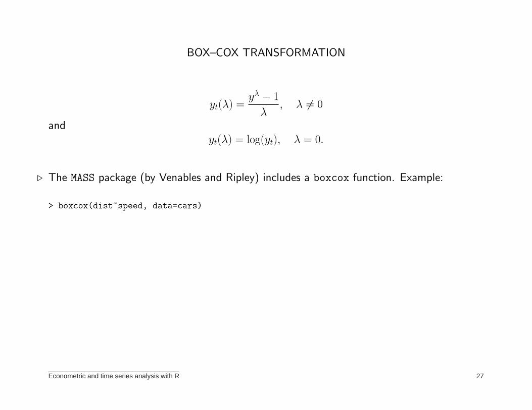
BOX–COX TRANSFORMATION

yt(λ) =yλ − 1

λ, λ 6= 0

andyt(λ) = log(yt), λ = 0.

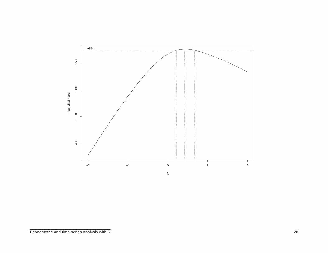
⊲ The MASS package (by Venables and Ripley) includes a boxcox function. Example:

> boxcox(dist~speed, data=cars)


−2 −1 0 1 2

−40

0−

350

−30

0−

250

λ

log−

Like

lihoo

d

95%


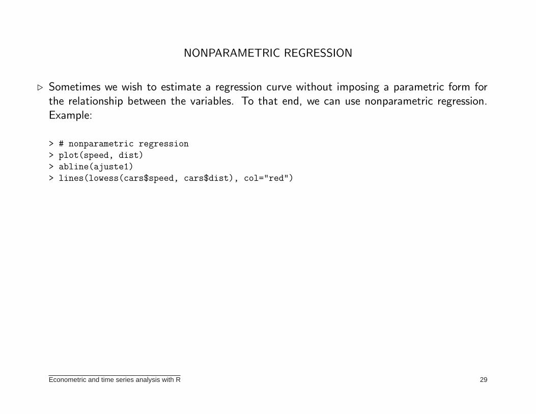
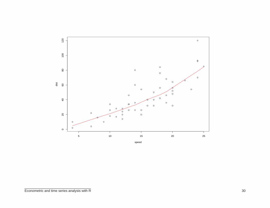
NONPARAMETRIC REGRESSION

⊲ Sometimes we wish to estimate a regression curve without imposing a parametric form forthe relationship between the variables. To that end, we can use nonparametric regression.Example:

> # nonparametric regression

> plot(speed, dist)

> abline(ajuste1)

> lines(lowess(cars$speed, cars$dist), col="red")


5 10 15 20 25

020

4060

8010

012

0

speed

dist


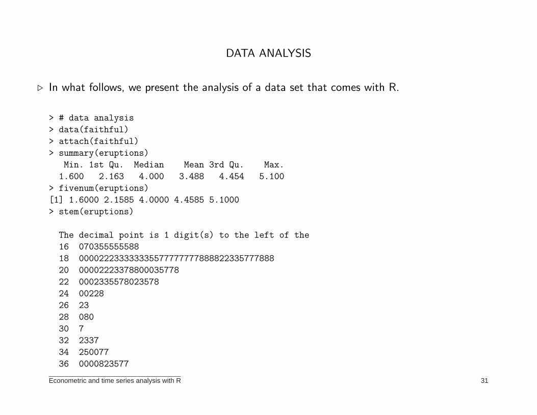
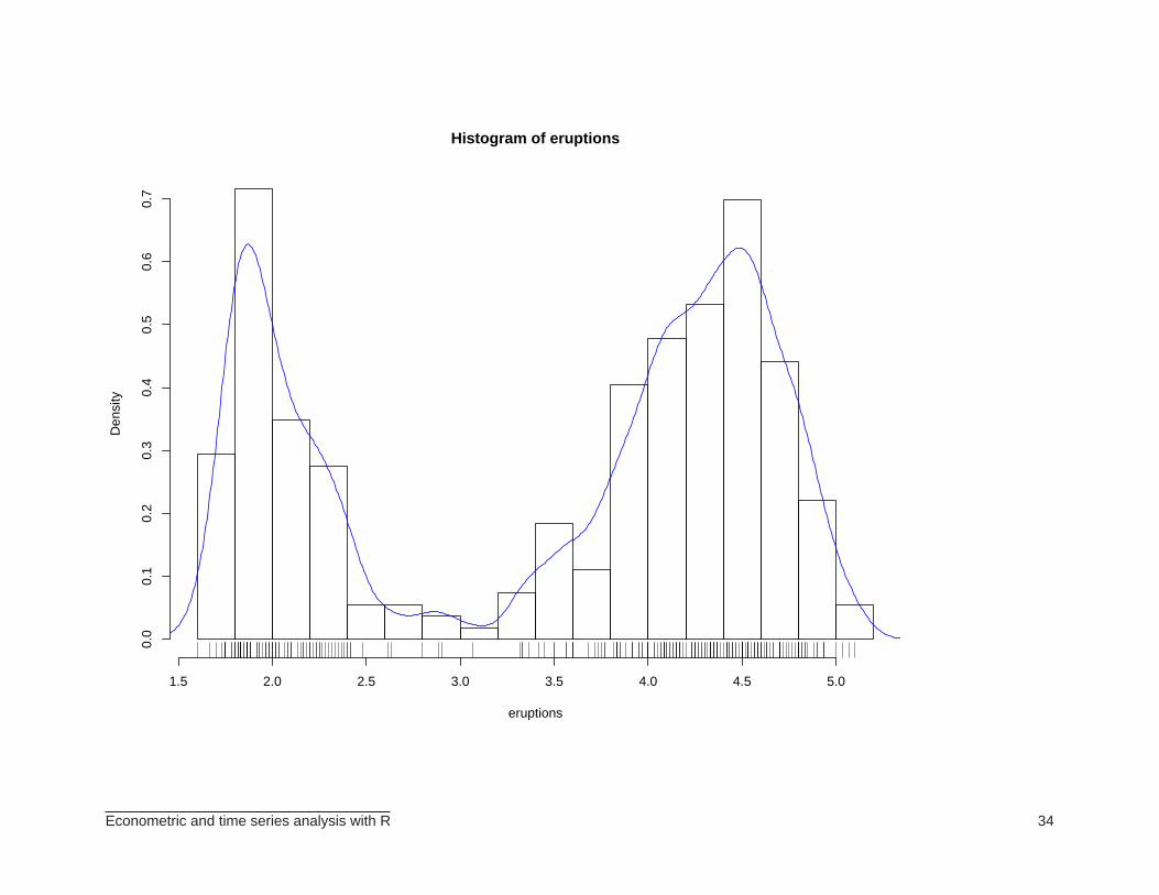
DATA ANALYSIS

⊲ In what follows, we present the analysis of a data set that comes with R.

> # data analysis

> data(faithful)

> attach(faithful)

> summary(eruptions)

Min. 1st Qu. Median Mean 3rd Qu. Max.

1.600 2.163 4.000 3.488 4.454 5.100

> fivenum(eruptions)

[1] 1.6000 2.1585 4.0000 4.4585 5.1000

> stem(eruptions)

The decimal point is 1 digit(s) to the left of the

16 070355555588

18 000022233333335577777777888822335777888

20 00002223378800035778

22 0002335578023578

24 00228

26 23

28 080

30 7

32 2337

34 250077

36 0000823577


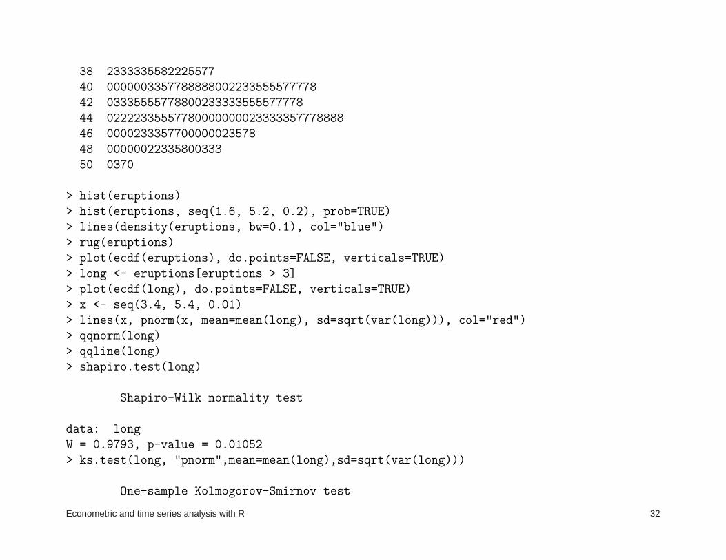
38 2333335582225577

40 0000003357788888002233555577778

42 03335555778800233333555577778

44 02222335557780000000023333357778888

46 0000233357700000023578

48 00000022335800333

50 0370

> hist(eruptions)

> hist(eruptions, seq(1.6, 5.2, 0.2), prob=TRUE)

> lines(density(eruptions, bw=0.1), col="blue")

> rug(eruptions)

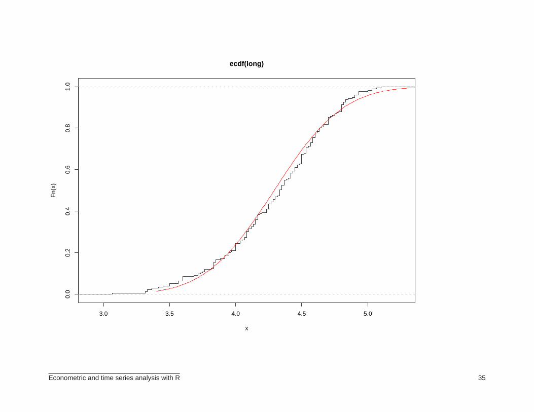
> plot(ecdf(eruptions), do.points=FALSE, verticals=TRUE)

> long <- eruptions[eruptions > 3]

> plot(ecdf(long), do.points=FALSE, verticals=TRUE)

> x <- seq(3.4, 5.4, 0.01)

> lines(x, pnorm(x, mean=mean(long), sd=sqrt(var(long))), col="red")

> qqnorm(long)

> qqline(long)

> shapiro.test(long)

Shapiro-Wilk normality test

data: long

W = 0.9793, p-value = 0.01052

> ks.test(long, "pnorm",mean=mean(long),sd=sqrt(var(long)))

One-sample Kolmogorov-Smirnov test


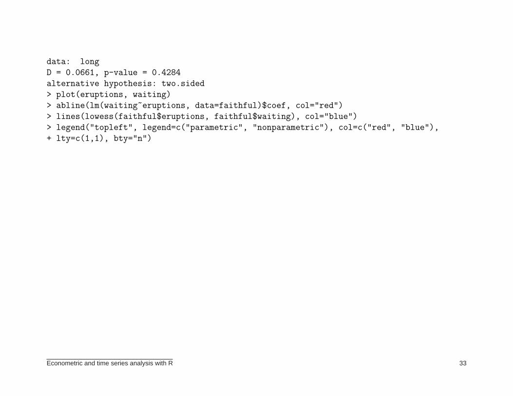
data: long

D = 0.0661, p-value = 0.4284

alternative hypothesis: two.sided

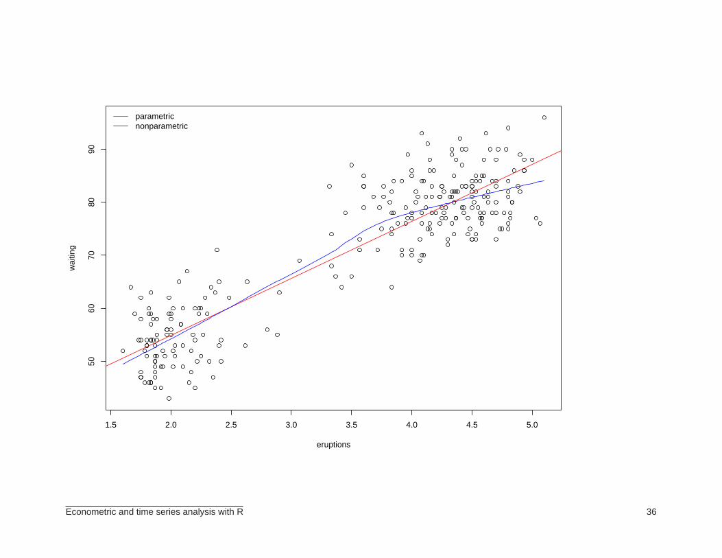
> plot(eruptions, waiting)

> abline(lm(waiting~eruptions, data=faithful)$coef, col="red")

> lines(lowess(faithful$eruptions, faithful$waiting), col="blue")

> legend("topleft", legend=c("parametric", "nonparametric"), col=c("red", "blue"),

+ lty=c(1,1), bty="n")


Histogram of eruptions

eruptions

Den

sity

1.5 2.0 2.5 3.0 3.5 4.0 4.5 5.0

0.0

0.1

0.2

0.3

0.4

0.5

0.6

0.7


3.0 3.5 4.0 4.5 5.0

0.0

0.2

0.4

0.6

0.8

1.0

ecdf(long)

x

Fn(

x)


1.5 2.0 2.5 3.0 3.5 4.0 4.5 5.0

5060

7080

90

eruptions

wai

ting

parametricnonparametric


NONLINEAR OPTIMIZATION

⊲ Statisticians and econometricians are often faced with the need to maximize or minimizefunctions (e.g., maximum likelihood estimation, least squares estimation, etc.). The nativeR function optim can be used to that end.

⊲ Methods supported by optim: BFGS, BFGS w/ box constraints, conjugate gradient, Nelder-Mead (default), simulated annealing.

⊲ Example: the Rosenbrock function:

f(x1, x2) = 100(x2 − x2

1)2 + (1 − x1)

2.

Suppose we wish to minimize this function with respect to x1 and x2.

⊲ We start by defining the function to be minimized and its gradient (if required):

fRosenbrock <- function(x)

{

100*(x[2]-x[1]*x[1])^2+(1-x[1])^2

}

gRosenbrock <- function(x)

{

c(-400*x[1]*(x[2]-x[1]*x[1])-2*(1-x[1]),

200*(x[2]-x[1]*x[1]))

}


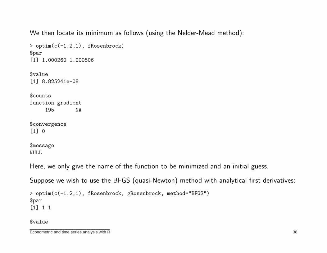
We then locate its minimum as follows (using the Nelder-Mead method):

> optim(c(-1.2,1), fRosenbrock)

$par

[1] 1.000260 1.000506

$value

[1] 8.825241e-08

$counts

function gradient

195 NA

$convergence

[1] 0

$message

NULL

Here, we only give the name of the function to be minimized and an initial guess.

Suppose we wish to use the BFGS (quasi-Newton) method with analytical first derivatives:

> optim(c(-1.2,1), fRosenbrock, gRosenbrock, method="BFGS")

$par

[1] 1 1

$value


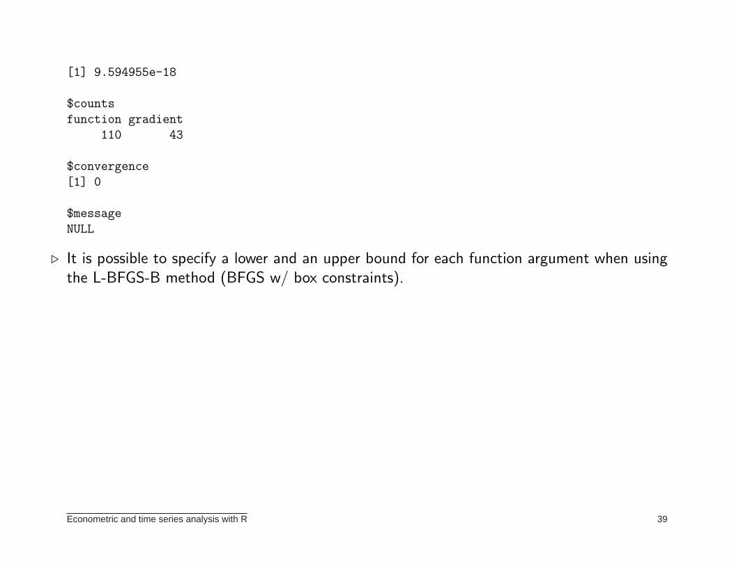
[1] 9.594955e-18

$counts

function gradient

110 43

$convergence

[1] 0

$message

NULL

⊲ It is possible to specify a lower and an upper bound for each function argument when usingthe L-BFGS-B method (BFGS w/ box constraints).


⊲ Suppose we now wish to locate the global minimum of a function that has several localminima. For the illustration, we shall consider:

f(x, y) = x2 + 2y2 −3

10cos(3πx) −

2

5cos(4πy) +

7

10.

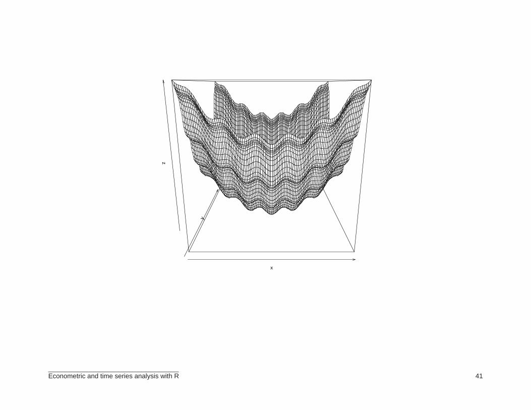
⊲ At the outset, plot the function:

> myfunction<-function(x,y)

+ {

+ x^2+2*y^2-(3/10)*cos(3*pi*x)-(2/5)*cos(4*pi*y)+(7/10)

+ }

>

> x <- y <-seq(-2,2,length=100)

> z <- outer(x,y,myfunction)

> persp(x,y,z)

> contour(x,y,z)

> image(x,y,z)


x

y

z


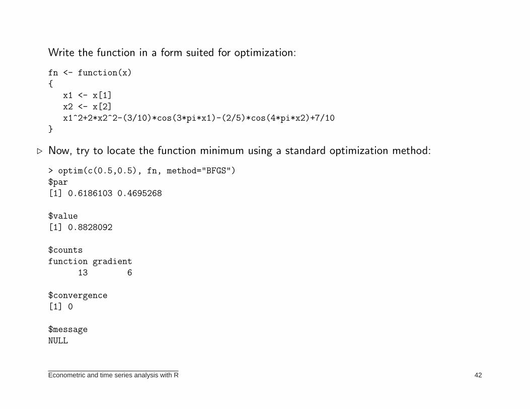
Write the function in a form suited for optimization:

fn <- function(x)

{

x1 <- x[1]

x2 <- x[2]

x1^2+2*x2^2-(3/10)*cos(3*pi*x1)-(2/5)*cos(4*pi*x2)+7/10

}

⊲ Now, try to locate the function minimum using a standard optimization method:

> optim(c(0.5,0.5), fn, method="BFGS")

$par

[1] 0.6186103 0.4695268

$value

[1] 0.8828092

$counts

function gradient

13 6

$convergence

[1] 0

$message

NULL


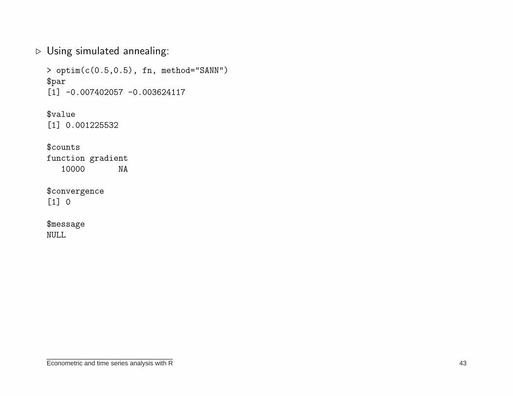
⊲ Using simulated annealing:

> optim(c(0.5,0.5), fn, method="SANN")

$par

[1] -0.007402057 -0.003624117

$value

[1] 0.001225532

$counts

function gradient

10000 NA

$convergence

[1] 0

$message

NULL


TIME SERIES

⊲ R contains several functions that are useful for time series analysis, such as:

◦ acf: sample autocorrelation and partial autocorrelation functions.◦ arima: estimation of ARMA, ARMAX, ARIMA, SARIMA models.◦ HoltWinters: prediction using seasonal (additive and multiplicative) and nonseasonal ex-

ponential smoothing methods (with optimal choice of the smoothing constants).◦ tsdiag: diagnostic tools for fitted ARIMA models.◦ etc. (Kalman filtering, theoretical autocorrelation functions, structural decomposition (stl),

spectral density estimation, unit root tests, and so on).

⊲ Additional functionality can be obtained by installing other packages, such as the dse andtseries packages (the former is for multivariate time series modeling; the latter containsfunctions for unit root test, BDS test, GARCH estimation, etc.). See also the urca anduroot packages for unit root and cointegration analysis, fracdiff for ARFIMA modeling,and dse for multivariate time series modeling.

⊲ A particularly useful package: forecast.

⊲ Use the function ts to format raw data as a time series; inform the begining period and thefrequency.


⊲ Example: simulation of time series (T = 200) from a stationary Gaussian AR(1) process.

> y = arima.sim(n=200, list(ar=0.5), innov=rnorm(200))

> plot.ts(y)


> plot.ts(y)


> plot.ts(y)


> plot.ts(y)

> acf(y) ## note the slow decay; we are close to nonstationary

> acf(diff(y))

⊲ Example: Wold decomposition.

> ARMAtoMA(ar=0.5, lag.max=30)

> ARMAtoMA(ar=0.95, lag.max=30) # note the slower decay


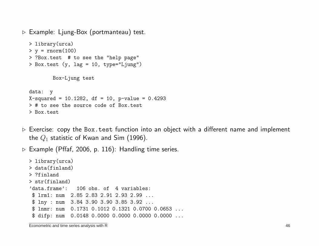
⊲ Example: Ljung-Box (portmanteau) test.

> library(urca)

> y = rnorm(100)

> ?Box.test # to see the "help page"

> Box.test (y, lag = 10, type="Ljung")

Box-Ljung test

data: y

X-squared = 10.1282, df = 10, p-value = 0.4293

> # to see the source code of Box.test

> Box.test

⊲ Exercise: copy the Box.test function into an object with a different name and implementthe Q1 statistic of Kwan and Sim (1996).

⊲ Example (Pffaf, 2006, p. 116): Handling time series.

> library(urca)

> data(finland)

> ?finland

> str(finland)

’data.frame’: 106 obs. of 4 variables:

$ lrm1: num 2.85 2.83 2.91 2.93 2.99 ...

$ lny : num 3.84 3.90 3.90 3.85 3.92 ...

$ lnmr: num 0.1731 0.1012 0.1321 0.0700 0.0653 ...

$ difp: num 0.0148 0.0000 0.0000 0.0000 0.0000 ...


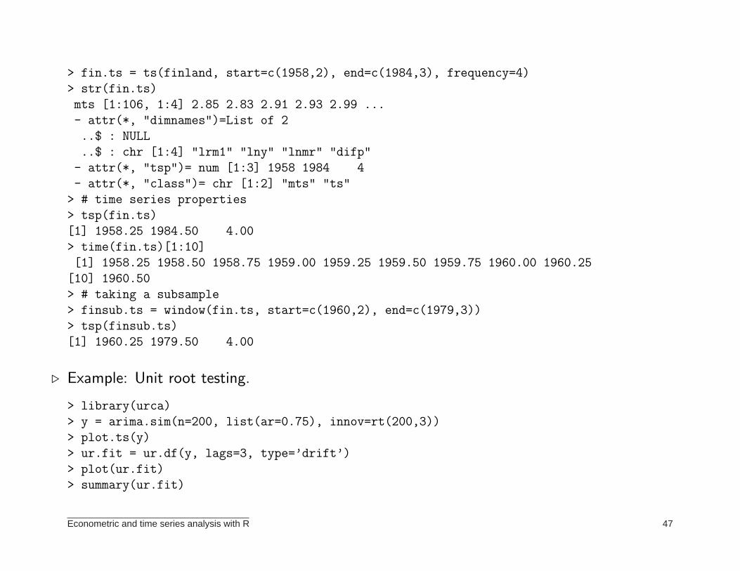
> fin.ts = ts(finland, start=c(1958,2), end=c(1984,3), frequency=4)

> str(fin.ts)

mts [1:106, 1:4] 2.85 2.83 2.91 2.93 2.99 ...

- attr(*, "dimnames")=List of 2

..$ : NULL

..$ : chr [1:4] "lrm1" "lny" "lnmr" "difp"

- attr(*, "tsp")= num [1:3] 1958 1984 4

- attr(*, "class")= chr [1:2] "mts" "ts"

> # time series properties

> tsp(fin.ts)

[1] 1958.25 1984.50 4.00

> time(fin.ts)[1:10]

[1] 1958.25 1958.50 1958.75 1959.00 1959.25 1959.50 1959.75 1960.00 1960.25

[10] 1960.50

> # taking a subsample

> finsub.ts = window(fin.ts, start=c(1960,2), end=c(1979,3))

> tsp(finsub.ts)

[1] 1960.25 1979.50 4.00

⊲ Example: Unit root testing.

> library(urca)

> y = arima.sim(n=200, list(ar=0.75), innov=rt(200,3))

> plot.ts(y)

> ur.fit = ur.df(y, lags=3, type=’drift’)

> plot(ur.fit)

> summary(ur.fit)


###############################################

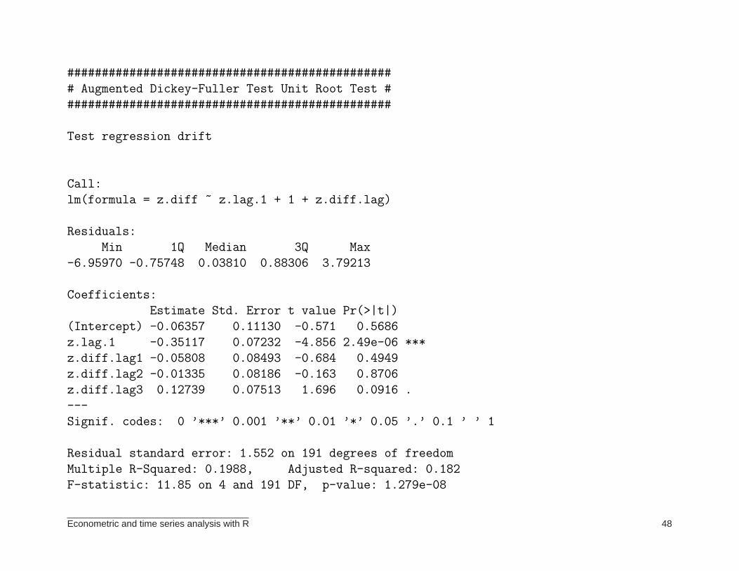
# Augmented Dickey-Fuller Test Unit Root Test #

###############################################

Test regression drift

Call:

lm(formula = z.diff ~ z.lag.1 + 1 + z.diff.lag)

Residuals:

Min 1Q Median 3Q Max

-6.95970 -0.75748 0.03810 0.88306 3.79213

Coefficients:

Estimate Std. Error t value Pr(>|t|)

(Intercept) -0.06357 0.11130 -0.571 0.5686

z.lag.1 -0.35117 0.07232 -4.856 2.49e-06 ***

z.diff.lag1 -0.05808 0.08493 -0.684 0.4949

z.diff.lag2 -0.01335 0.08186 -0.163 0.8706

z.diff.lag3 0.12739 0.07513 1.696 0.0916 .

---

Signif. codes: 0 ’***’ 0.001 ’**’ 0.01 ’*’ 0.05 ’.’ 0.1 ’ ’ 1

Residual standard error: 1.552 on 191 degrees of freedom

Multiple R-Squared: 0.1988, Adjusted R-squared: 0.182

F-statistic: 11.85 on 4 and 191 DF, p-value: 1.279e-08


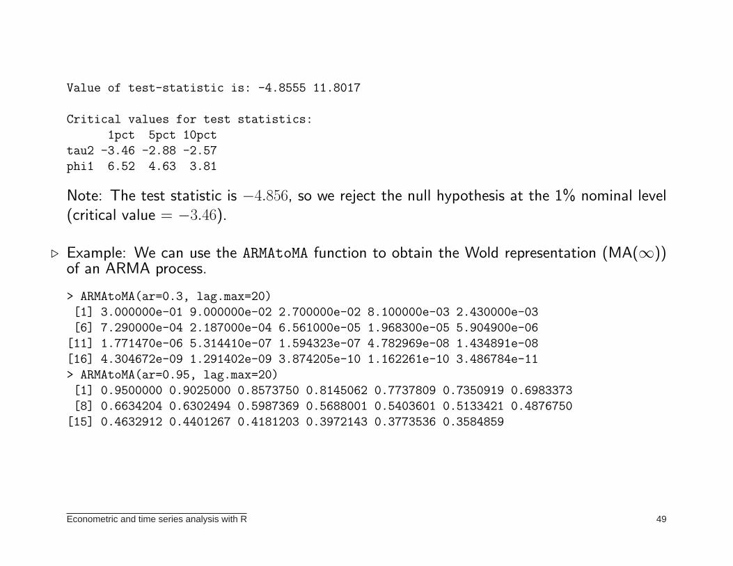
Value of test-statistic is: -4.8555 11.8017

Critical values for test statistics:

1pct 5pct 10pct

tau2 -3.46 -2.88 -2.57

phi1 6.52 4.63 3.81

Note: The test statistic is −4.856, so we reject the null hypothesis at the 1% nominal level(critical value = −3.46).

⊲ Example: We can use the ARMAtoMA function to obtain the Wold representation (MA(∞))of an ARMA process.


[1] 3.000000e-01 9.000000e-02 2.700000e-02 8.100000e-03 2.430000e-03

[6] 7.290000e-04 2.187000e-04 6.561000e-05 1.968300e-05 5.904900e-06

[11] 1.771470e-06 5.314410e-07 1.594323e-07 4.782969e-08 1.434891e-08

[16] 4.304672e-09 1.291402e-09 3.874205e-10 1.162261e-10 3.486784e-11


[1] 0.9500000 0.9025000 0.8573750 0.8145062 0.7737809 0.7350919 0.6983373

[8] 0.6634204 0.6302494 0.5987369 0.5688001 0.5403601 0.5133421 0.4876750

[15] 0.4632912 0.4401267 0.4181203 0.3972143 0.3773536 0.3584859


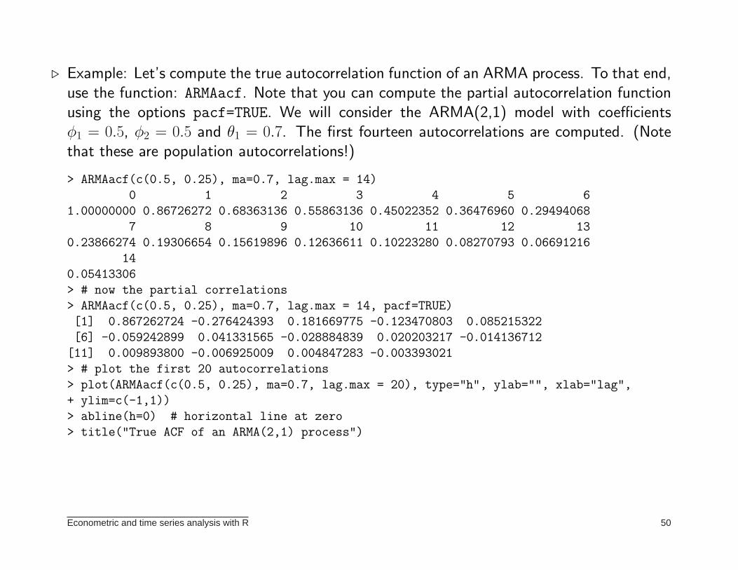
⊲ Example: Let’s compute the true autocorrelation function of an ARMA process. To that end,use the function: ARMAacf. Note that you can compute the partial autocorrelation functionusing the options pacf=TRUE. We will consider the ARMA(2,1) model with coefficientsφ1 = 0.5, φ2 = 0.5 and θ1 = 0.7. The first fourteen autocorrelations are computed. (Notethat these are population autocorrelations!)

> ARMAacf(c(0.5, 0.25), ma=0.7, lag.max = 14)

0 1 2 3 4 5 6

1.00000000 0.86726272 0.68363136 0.55863136 0.45022352 0.36476960 0.29494068

7 8 9 10 11 12 13

0.23866274 0.19306654 0.15619896 0.12636611 0.10223280 0.08270793 0.06691216

14

0.05413306

> # now the partial correlations

> ARMAacf(c(0.5, 0.25), ma=0.7, lag.max = 14, pacf=TRUE)

[1] 0.867262724 -0.276424393 0.181669775 -0.123470803 0.085215322

[6] -0.059242899 0.041331565 -0.028884839 0.020203217 -0.014136712

[11] 0.009893800 -0.006925009 0.004847283 -0.003393021

> # plot the first 20 autocorrelations

> plot(ARMAacf(c(0.5, 0.25), ma=0.7, lag.max = 20), type="h", ylab="", xlab="lag",

+ ylim=c(-1,1))

> abline(h=0) # horizontal line at zero

> title("True ACF of an ARMA(2,1) process")


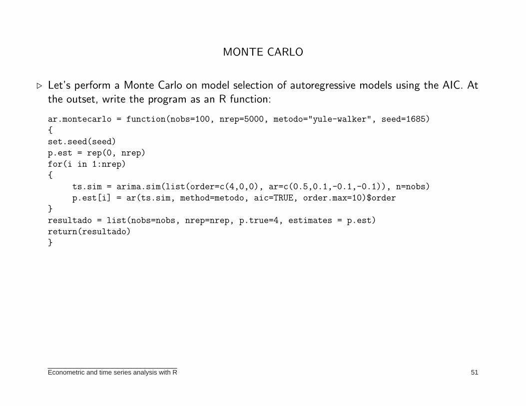
MONTE CARLO

⊲ Let’s perform a Monte Carlo on model selection of autoregressive models using the AIC. Atthe outset, write the program as an R function:

ar.montecarlo = function(nobs=100, nrep=5000, metodo="yule-walker", seed=1685)

{

set.seed(seed)

p.est = rep(0, nrep)

for(i in 1:nrep)

{

ts.sim = arima.sim(list(order=c(4,0,0), ar=c(0.5,0.1,-0.1,-0.1)), n=nobs)

p.est[i] = ar(ts.sim, method=metodo, aic=TRUE, order.max=10)$order

}

resultado = list(nobs=nobs, nrep=nrep, p.true=4, estimates = p.est)

return(resultado)

}


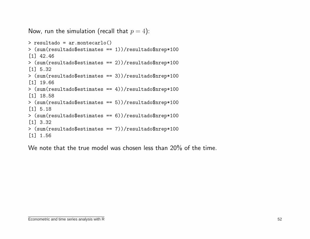
Now, run the simulation (recall that p = 4):

> resultado = ar.montecarlo()

> (sum(resultado$estimates == 1))/resultado$nrep*100

[1] 42.46


[1] 5.32


[1] 19.66


[1] 18.58


[1] 5.18


[1] 3.32


[1] 1.56

We note that the true model was chosen less than 20% of the time.


Econometric and time series modeling using R - UFPE

Documents

Transcript of Econometric and time series modeling using R - UFPE