ECON 4551 Econometrics II Memorial University of...
74
Panel Data Models Adapted from Vera Tabakova’s notes ECON 4551 Econometrics II Memorial University of Newfoundland
Transcript of ECON 4551 Econometrics II Memorial University of...
Panel Data Models
Adapted from Vera Tabakova’s notes
ECON 4551 Econometrics II Memorial University of Newfoundland
15.1 Grunfeld’s Investment Data
15.2 Sets of Regression Equations
15.3 Seemingly Unrelated Regressions
15.4 The Fixed Effects Model
15.4 The Random Effects Model
Extensions RCM, dealing with endogeneity when we have
static variables
Slide 15-2 Principles of Econometrics, 3rd Edition
The different types of panel data sets can be described as:
“long and narrow,” with “long” time dimension and “narrow”, few
cross sectional units;
“short and wide,” many units observed over a short period of time;
“long and wide,” indicating that both N and T are relatively large.
Slide 15-3 Principles of Econometrics, 3rd Edition
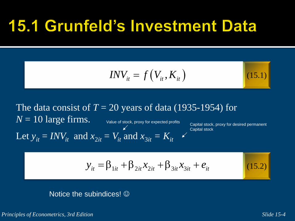
The data consist of T = 20 years of data (1935-1954) for N = 10 large firms.
Let yit = INVit and x2it = Vit and x3it = Kit
Slide 15-4 Principles of Econometrics, 3rd Edition
(15.1)
(15.2)
( ),it it itINV f V K=
1 2 2 3 3it it it it it it ity x x e= β +β +β +
Notice the subindices!
Value of stock, proxy for expected profits Capital stock, proxy for desired permanent Capital stock
Slide 15-5 Principles of Econometrics, 3rd Edition
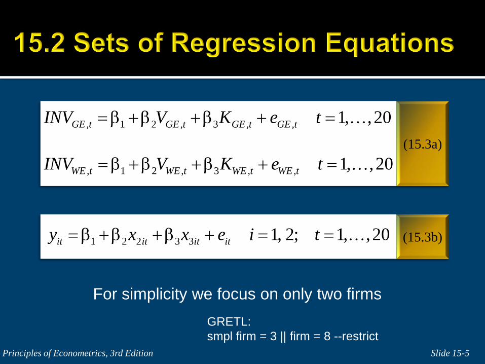
(15.3a)
(15.3b)
, 1 2 , 3 , ,
, 1 2 , 3 , ,
1, ,20
1, ,20
GE t GE t GE t GE t
WE t WE t WE t WE t
INV V K e t
INV V K e t
= β +β +β + =
= β +β +β + =
1 2 2 3 3 1, 2; 1, ,20it it it ity x x e i t= β +β +β + = =
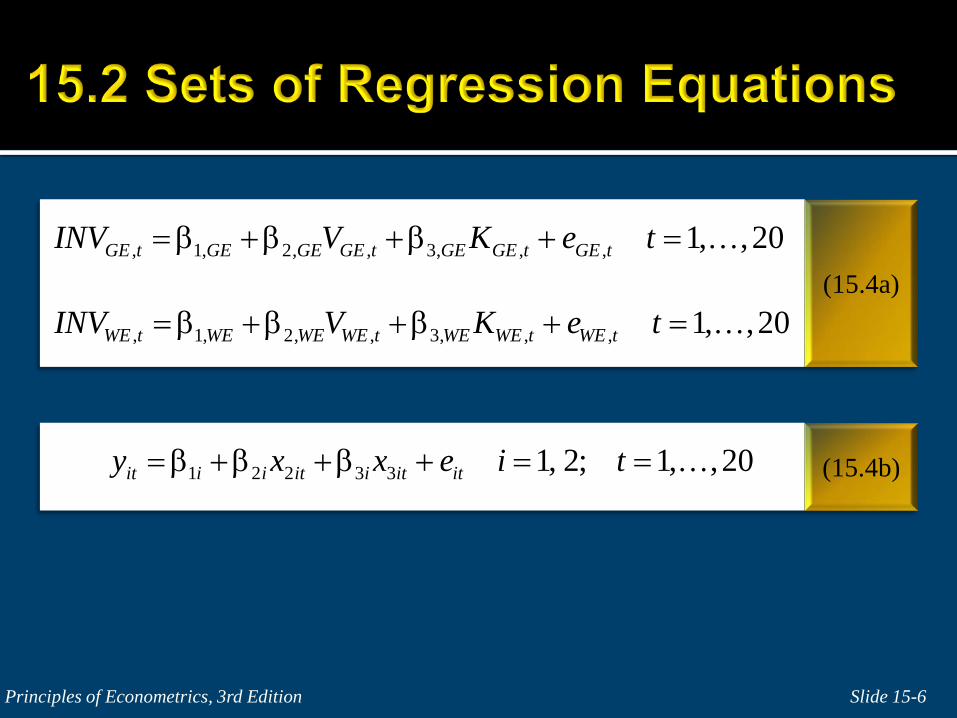
For simplicity we focus on only two firms
GRETL: smpl firm = 3 || firm = 8 --restrict
Slide 15-6 Principles of Econometrics, 3rd Edition
(15.4a)
(15.4b)
, 1, 2, , 3, , ,
, 1, 2, , 3, , ,
1, ,20
1, ,20
GE t GE GE GE t GE GE t GE t
WE t WE WE WE t WE WE t WE t
INV V K e t
INV V K e t
= β +β +β + =
= β +β +β + =
1 2 2 3 3 1, 2; 1, ,20it i i it i it ity x x e i t= β +β +β + = =
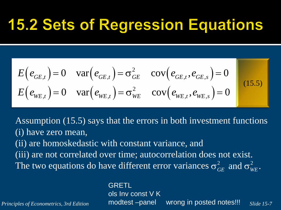
Assumption (15.5) says that the errors in both investment functions
(i) have zero mean, (ii) are homoskedastic with constant variance, and (iii) are not correlated over time; autocorrelation does not exist. The two equations do have different error variances
Slide 15-7 Principles of Econometrics, 3rd Edition
(15.5) ( ) ( ) ( )( ) ( ) ( )
2, , , ,
2, , , ,
0 var cov , 0
0 var cov , 0GE t GE t GE GE t GE s
WE t WE t WE WE t WE s
E e e e e
E e e e e
= = σ =
= = σ =
2 2 and .GE WEσ σ
GRETL ols Inv const V K modtest –panel wrong in posted notes!!!

Slide 15-8 Principles of Econometrics, 3rd Edition
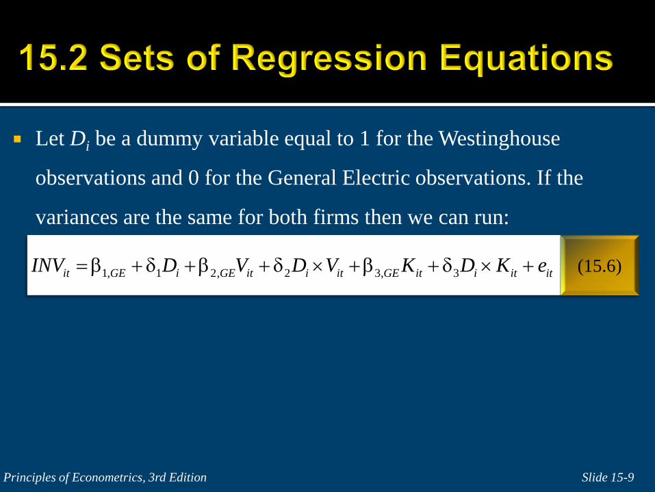
Let Di be a dummy variable equal to 1 for the Westinghouse
observations and 0 for the General Electric observations. If the
variances are the same for both firms then we can run:
Slide 15-9 Principles of Econometrics, 3rd Edition
(15.6) 1, 1 2, 2 3, 3it GE i GE it i it GE it i it itINV D V D V K D K e= β + δ +β + δ × +β + δ × +
Slide 15-10 Principles of Econometrics, 3rd Edition
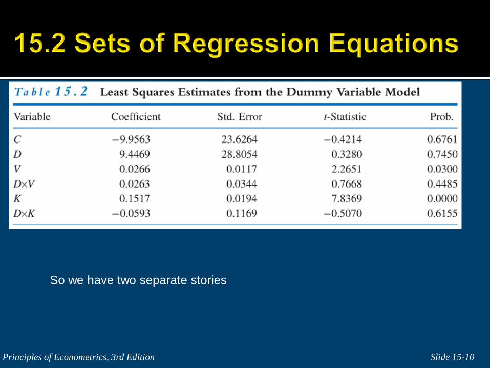
So we have two separate stories
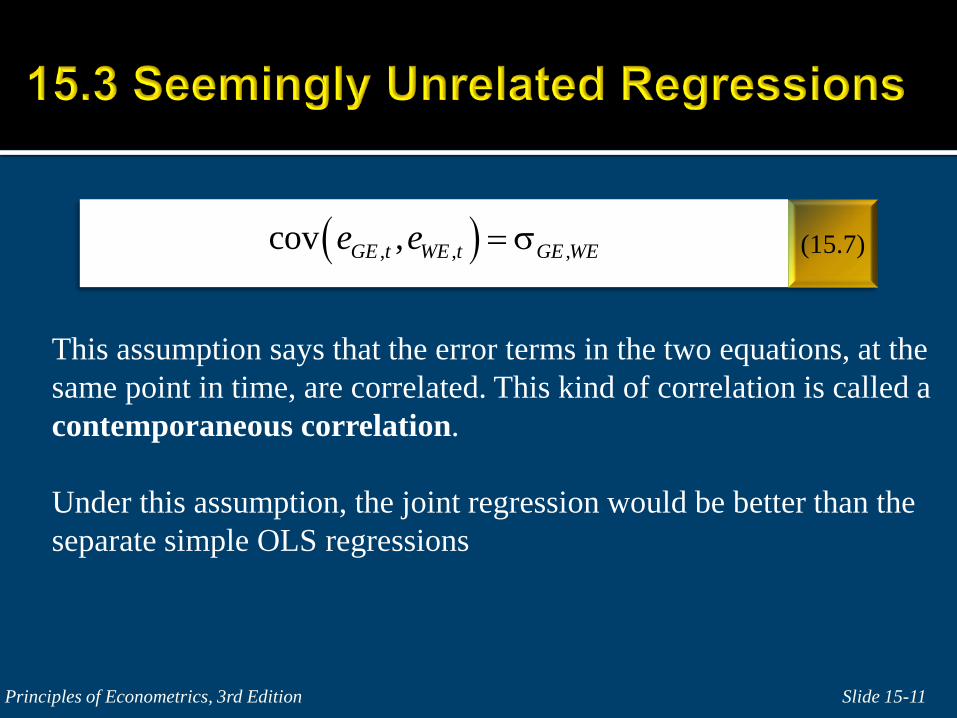
This assumption says that the error terms in the two equations, at the same point in time, are correlated. This kind of correlation is called a contemporaneous correlation.
Under this assumption, the joint regression would be better than the
separate simple OLS regressions
Slide 15-11 Principles of Econometrics, 3rd Edition
(15.7) ( ), , ,cov ,GE t WE t GE WEe e = σ
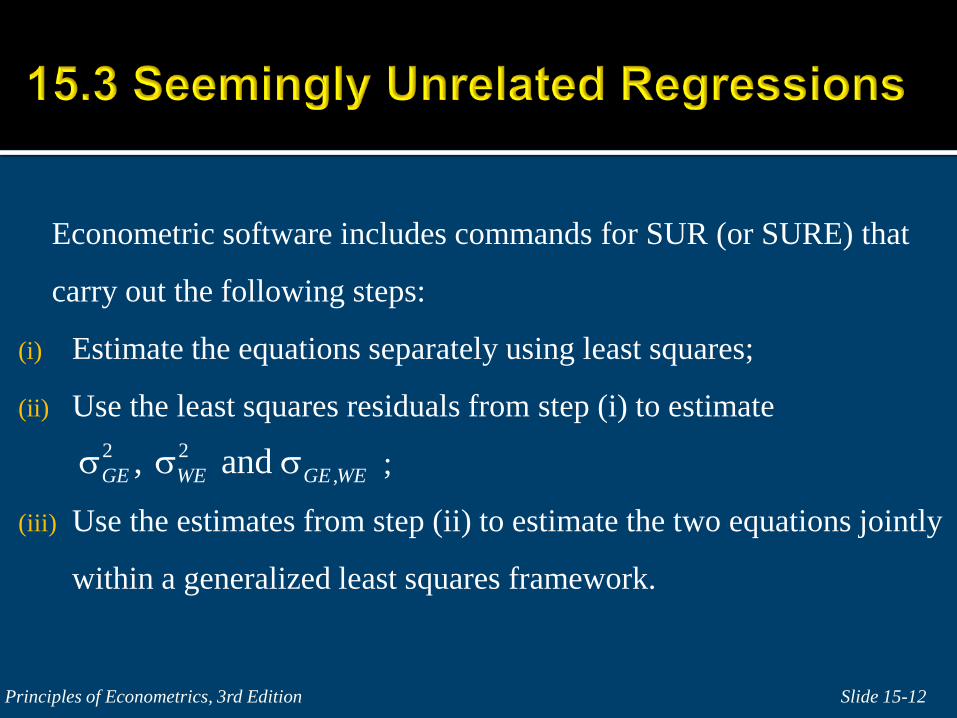
Econometric software includes commands for SUR (or SURE) that
carry out the following steps:
(i) Estimate the equations separately using least squares;
(ii) Use the least squares residuals from step (i) to estimate
;
(iii) Use the estimates from step (ii) to estimate the two equations jointly
within a generalized least squares framework.
Slide 15-12 Principles of Econometrics, 3rd Edition
2 2,, and GE WE GE WEσ σ σ
Slide 15-13 Principles of Econometrics, 3rd Edition
Slide 15-14 Principles of Econometrics, 3rd Edition
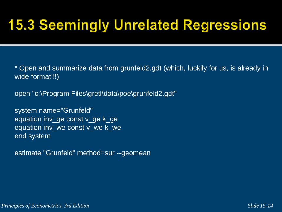
* Open and summarize data from grunfeld2.gdt (which, luckily for us, is already in wide format!!!) open "c:\Program Files\gretl\data\poe\grunfeld2.gdt" system name="Grunfeld" equation inv_ge const v_ge k_ge equation inv_we const v_we k_we end system estimate "Grunfeld" method=sur --geomean
Slide 15-15 Principles of Econometrics, 3rd Edition
In GRETL the restrict command can be used to impose the cross-equation restrictions on a system of equations that has been previously defined and named. The set of restrictions is started by restrict and terminated with end restrict. Each restriction in the set is expressed as an equation. Put the linear combination of parameters to be tested on the left-hand-side of the equality and a numeric value on the right. Parameters are referenced using b[i,j] where i refers to the equation number in the system, and j the parameter number.
Slide 15-16 Principles of Econometrics, 3rd Edition
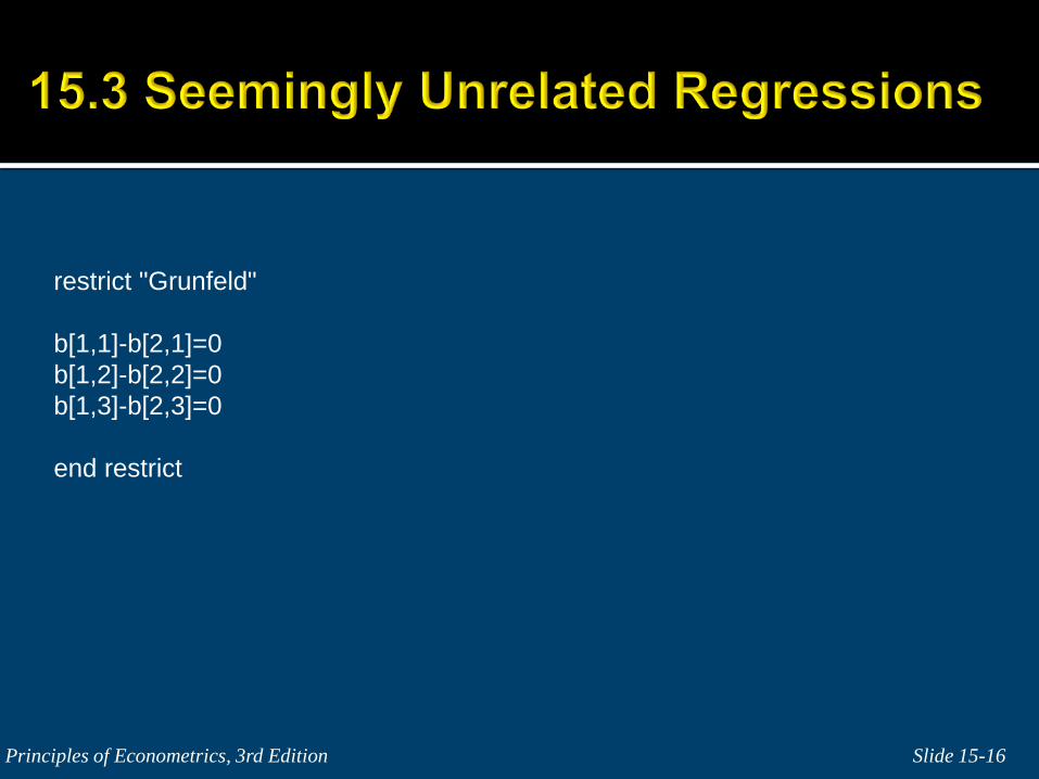
restrict "Grunfeld" b[1,1]-b[2,1]=0 b[1,2]-b[2,2]=0 b[1,3]-b[2,3]=0 end restrict
There are two situations where separate least squares estimation is
just as good as the SUR technique :
(i) when the equation errors are not contemporaneously correlated;
(ii) when the same (the “very same”) explanatory variables appear in
each equation.
If the explanatory variables in each equation are different, then a test
to see if the correlation between the errors is significantly different
from zero is of interest. Slide 15-17 Principles of Econometrics, 3rd Edition
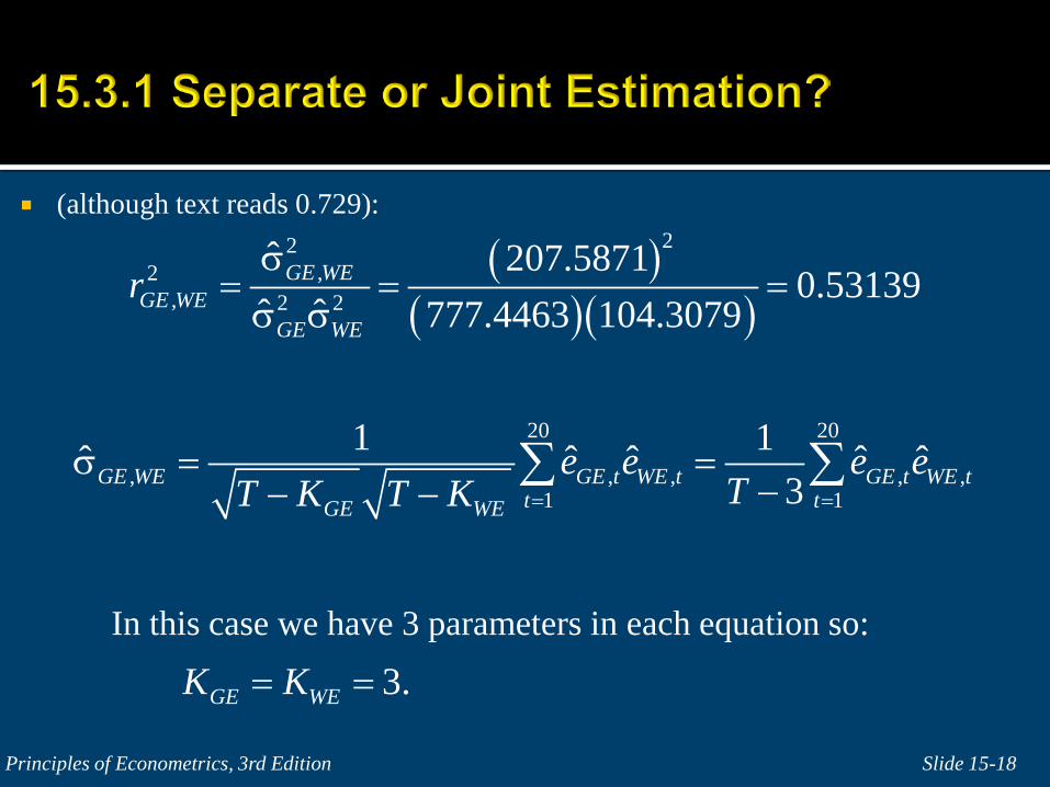
(although text reads 0.729):
In this case we have 3 parameters in each equation so:
Slide 15-18 Principles of Econometrics, 3rd Edition
( )( )( )
22,2
, 2 2
ˆ 207.58710.53139
ˆ ˆ 777.4463 104.3079GE WE
GE WEGE WE
rσ
= = =σ σ
20 20
, , , , ,1 1
1 1ˆ ˆ ˆ ˆ ˆ3GE WE GE t WE t GE t WE t
t tGE WE
e e e eTT K T K = =
σ = =−− −
∑ ∑
3.GE WEK K= =
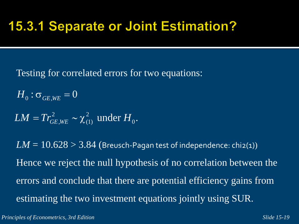
Testing for correlated errors for two equations:
LM = 10.628 > 3.84 (Breusch-Pagan test of independence: chi2(1))
Hence we reject the null hypothesis of no correlation between the
errors and conclude that there are potential efficiency gains from
estimating the two investment equations jointly using SUR.
Slide 15-19 Principles of Econometrics, 3rd Edition
0 ,: 0GE WEH σ =
2 2, (1) 0 under .GE WELM Tr H= ∼ χ
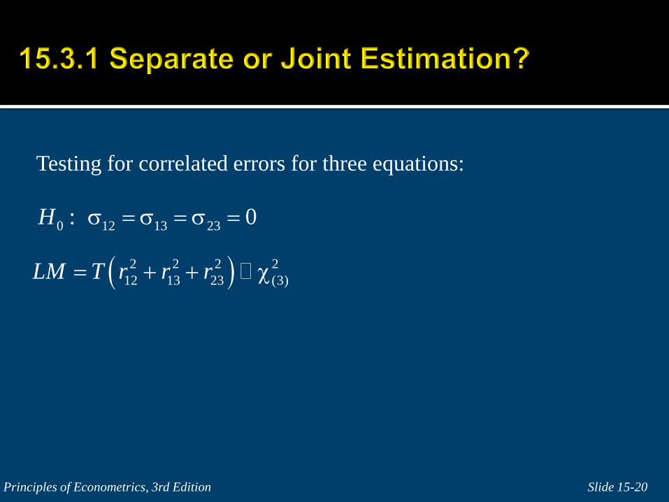
Testing for correlated errors for three equations:
Slide 15-20 Principles of Econometrics, 3rd Edition
0 12 13 23: 0H σ = σ = σ =
( )2 2 2 212 13 23 (3)LM T r r r= + + χ
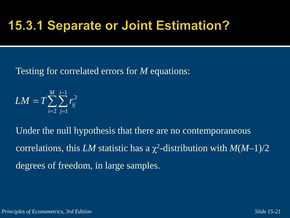
Testing for correlated errors for M equations:
Under the null hypothesis that there are no contemporaneous
correlations, this LM statistic has a χ2-distribution with M(M–1)/2
degrees of freedom, in large samples.
Slide 15-21 Principles of Econometrics, 3rd Edition
12
2 1
M i
iji j
LM T r−
= == ∑∑
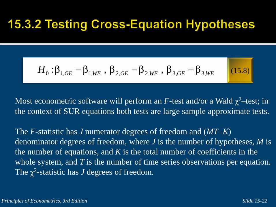
Most econometric software will perform an F-test and/or a Wald χ2–test; in the context of SUR equations both tests are large sample approximate tests.
The F-statistic has J numerator degrees of freedom and (MT−K)
denominator degrees of freedom, where J is the number of hypotheses, M is the number of equations, and K is the total number of coefficients in the whole system, and T is the number of time series observations per equation. The χ2-statistic has J degrees of freedom.
Slide 15-22 Principles of Econometrics, 3rd Edition
(15.8) 0 1, 1, 2, 2, 3, 3,: , ,GE WE GE WE GE WEH β = β β = β β = β
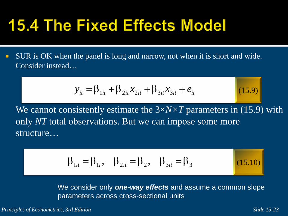
SUR is OK when the panel is long and narrow, not when it is short and wide. Consider instead…
We cannot consistently estimate the 3×N×T parameters in (15.9) with only NT total observations. But we can impose some more structure…
Slide 15-23 Principles of Econometrics, 3rd Edition
(15.9)
(15.10)
1 2 2 3 3it it it it it it ity x x e= β +β +β +
1 1 2 2 3 3, ,it i it itβ = β β = β β = β
We consider only one-way effects and assume a common slope parameters across cross-sectional units
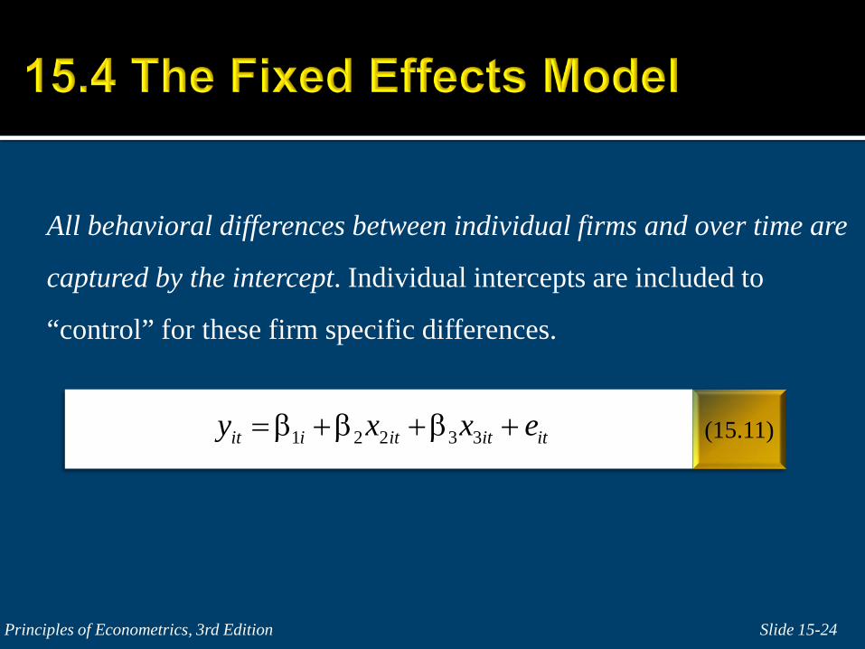
All behavioral differences between individual firms and over time are
captured by the intercept. Individual intercepts are included to
“control” for these firm specific differences.
Slide 15-24 Principles of Econometrics, 3rd Edition
(15.11) 1 2 2 3 3it i it it ity x x e= β +β +β +
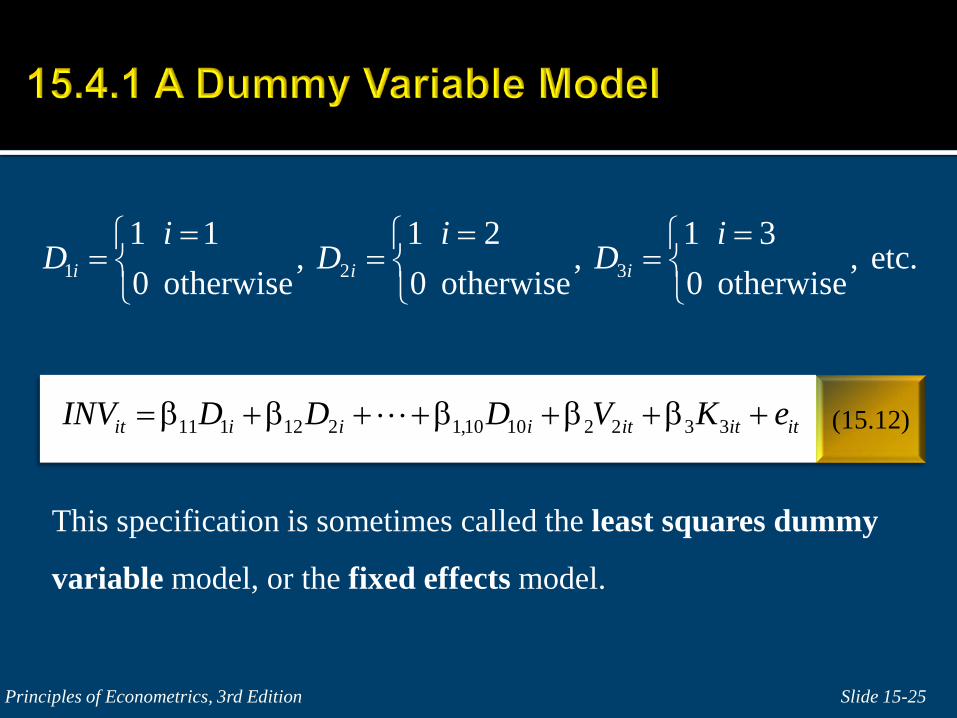
This specification is sometimes called the least squares dummy
variable model, or the fixed effects model.
Slide 15-25 Principles of Econometrics, 3rd Edition
(15.12)
1 2 3
1 1 1 2 1 3, , , etc.
0 otherwise 0 otherwise 0 otherwisei i i
i i iD D D
= = = = = =
11 1 12 2 1,10 10 2 2 3 3it i i i it it itINV D D D V K e= β +β + +β +β +β +
Slide 15-26 Principles of Econometrics, 3rd Edition
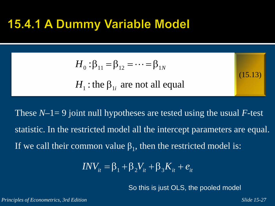
These N–1= 9 joint null hypotheses are tested using the usual F-test
statistic. In the restricted model all the intercept parameters are equal.
If we call their common value β1, then the restricted model is:
Slide 15-27 Principles of Econometrics, 3rd Edition
(15.13) 0 11 12 1
1 1
:
: the are not all equal
N
i
H
H
β = β = = β
β
1 2 3it it it itINV V K e= β +β +β +
So this is just OLS, the pooled model
Slide 15-28 Principles of Econometrics, 3rd Edition
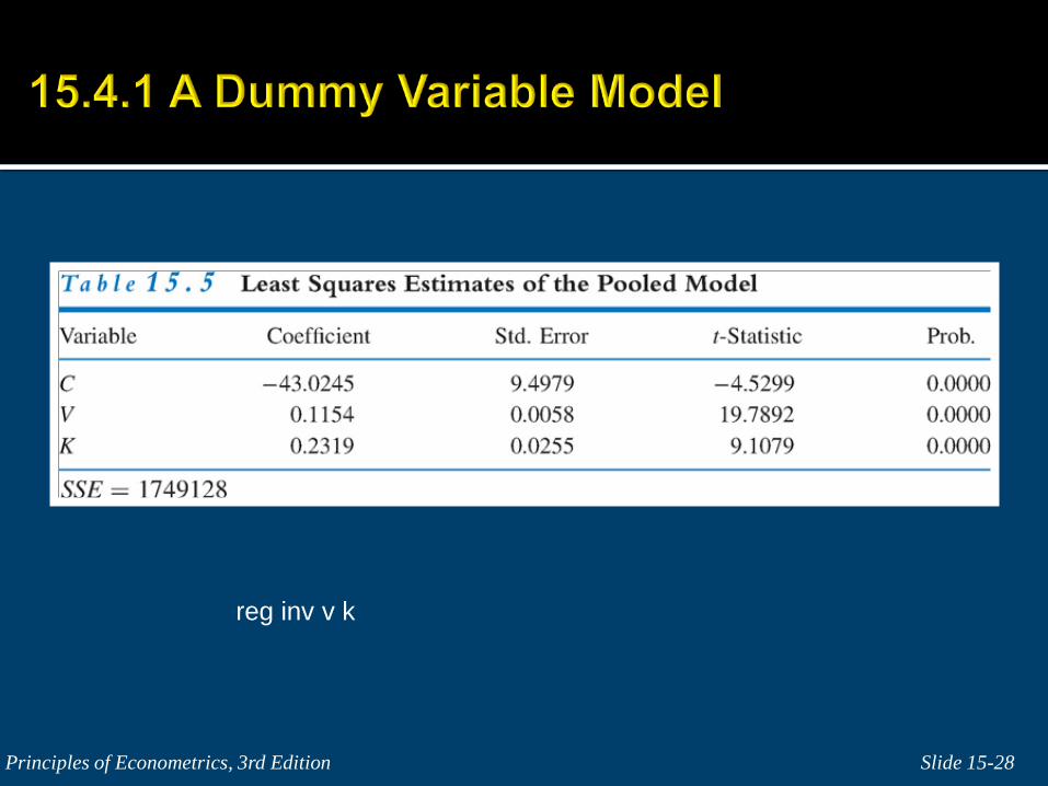
reg inv v k
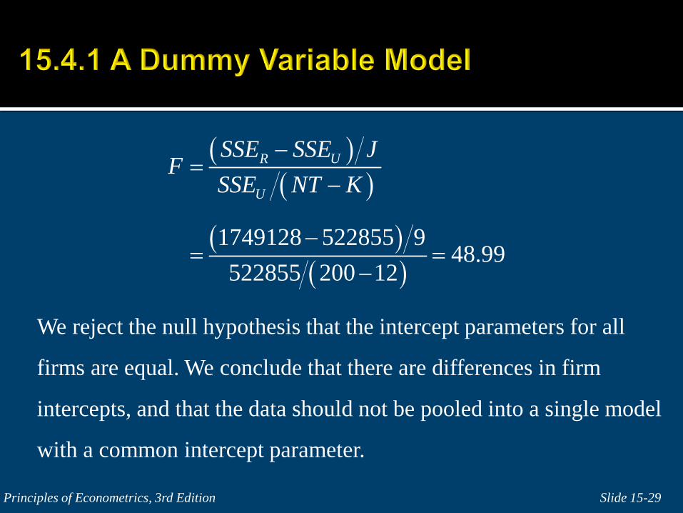
We reject the null hypothesis that the intercept parameters for all
firms are equal. We conclude that there are differences in firm
intercepts, and that the data should not be pooled into a single model
with a common intercept parameter.
Slide 15-29 Principles of Econometrics, 3rd Edition
( )( )
( )( )
1749128 522855 948.99
522855 200 12
R U
U
SSE SSE JF
SSE NT K−
=−
−= =
−
Slide 15-30 Principles of Econometrics, 3rd Edition
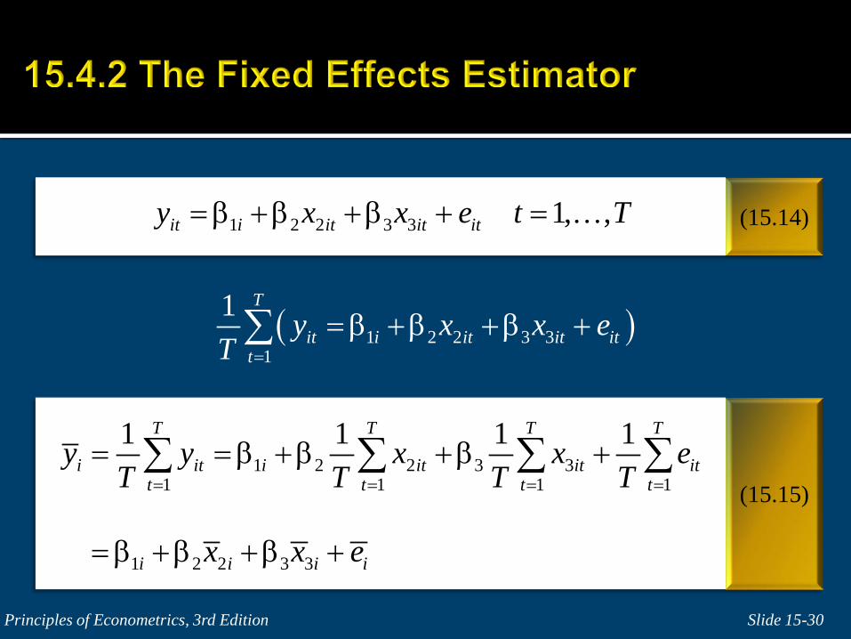
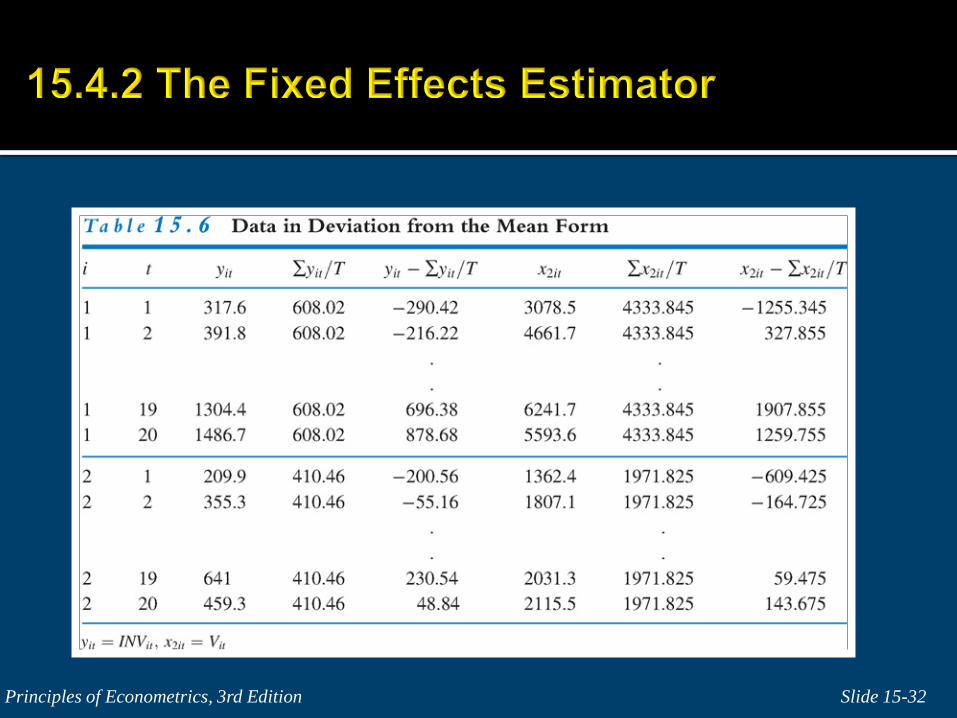
(15.14) 1 2 2 3 3 1, ,it i it it ity x x e t T= β +β +β + =
(15.15)
( )1 2 2 3 31
1 T
it i it it itt
y x x eT =
= β +β +β +∑
1 2 2 3 31 1 1 1
1 2 2 3 3
1 1 1 1T T T T
i it i it it itt t t t
i i i i
y y x x eT T T T
x x e
= = = == = β +β +β +
= β +β +β +
∑ ∑ ∑ ∑
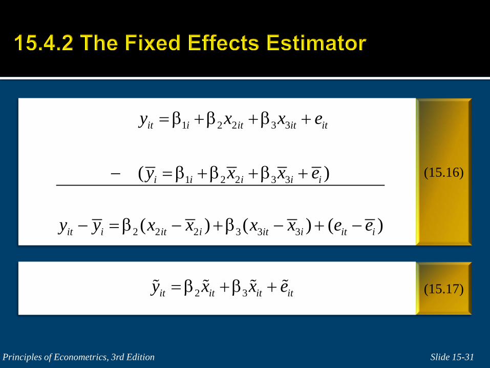
Slide 15-31 Principles of Econometrics, 3rd Edition
(15.16)
1 2 2 3 3
1 2 2 3 3
2 2 2 3 3 3
( )
( ) ( ) ( )
it i it it it
i i i i i
it i it i it i it i
y x x e
y x x e
y y x x x x e e
= β +β +β +
− = β +β +β +
− = β − +β − + −
(15.17) 2 3it it it ity x x e= β +β +
Slide 15-32 Principles of Econometrics, 3rd Edition
Slide 15-33 Principles of Econometrics, 3rd Edition
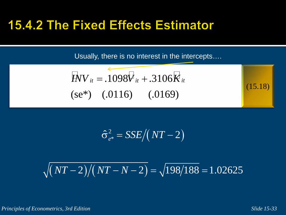
(15.18) .1098 .3106(se*) (.0116) (.0169)
itit itINV V K= +
( )2*ˆ 2e SSE NTσ = −
( ) ( )2 2 198 188 1.02625NT NT N− − − = =
Usually, there is no interest in the intercepts….
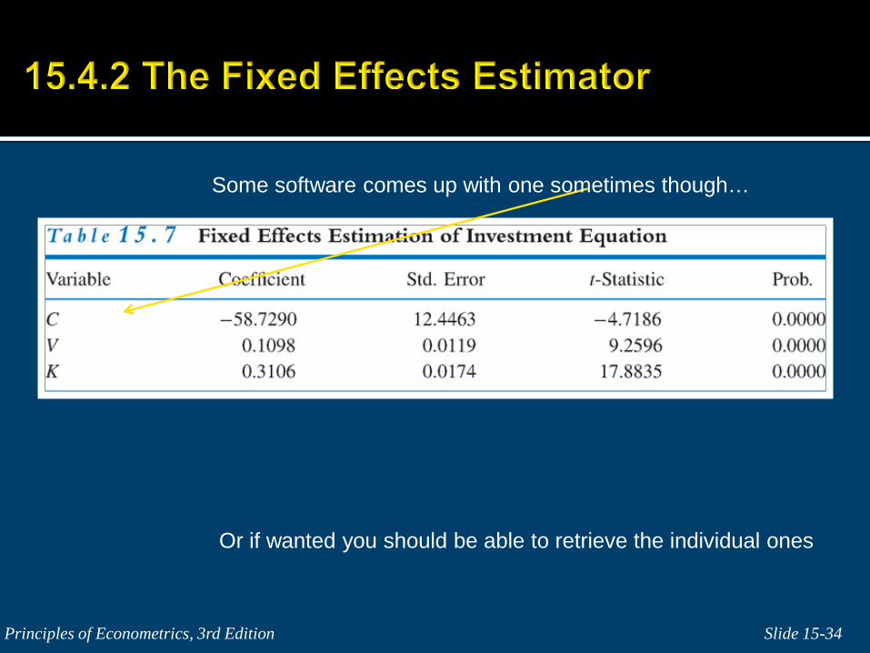
Slide 15-34 Principles of Econometrics, 3rd Edition
Some software comes up with one sometimes though…
Or if wanted you should be able to retrieve the individual ones
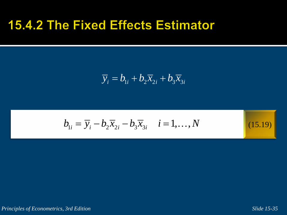
Slide 15-35 Principles of Econometrics, 3rd Edition
(15.19)
1 2 2 3 3i i i iy b b x b x= + +
1 2 2 3 3 1, ,i i i ib y b x b x i N= − − =
Slide 15-36 Principles of Econometrics, 3rd Edition
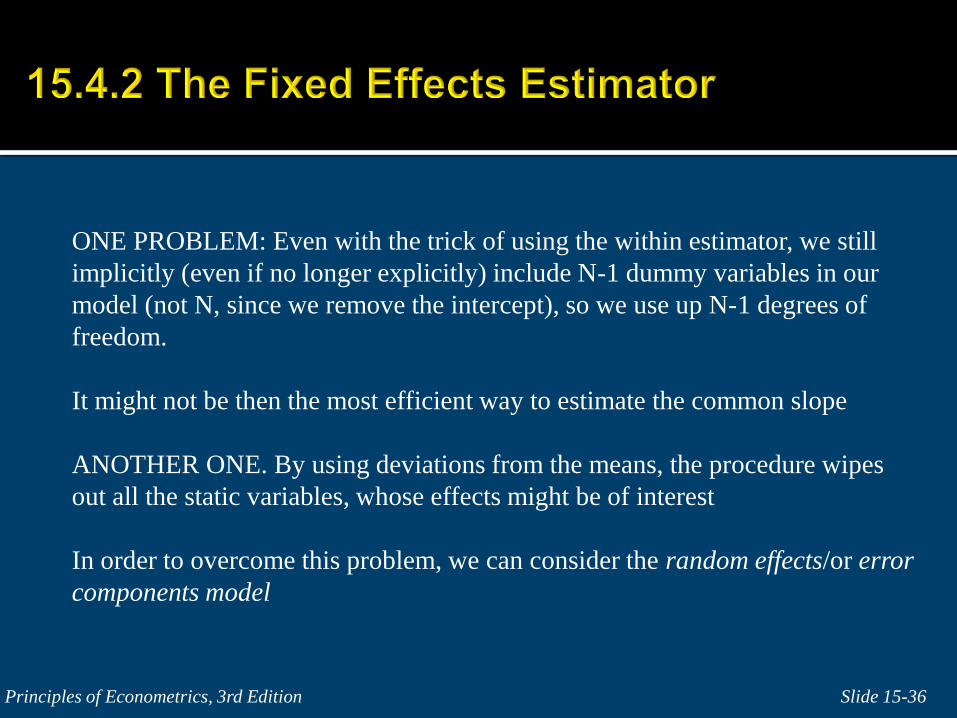
ONE PROBLEM: Even with the trick of using the within estimator, we still implicitly (even if no longer explicitly) include N-1 dummy variables in our model (not N, since we remove the intercept), so we use up N-1 degrees of freedom. It might not be then the most efficient way to estimate the common slope ANOTHER ONE. By using deviations from the means, the procedure wipes out all the static variables, whose effects might be of interest In order to overcome this problem, we can consider the random effects/or error components model
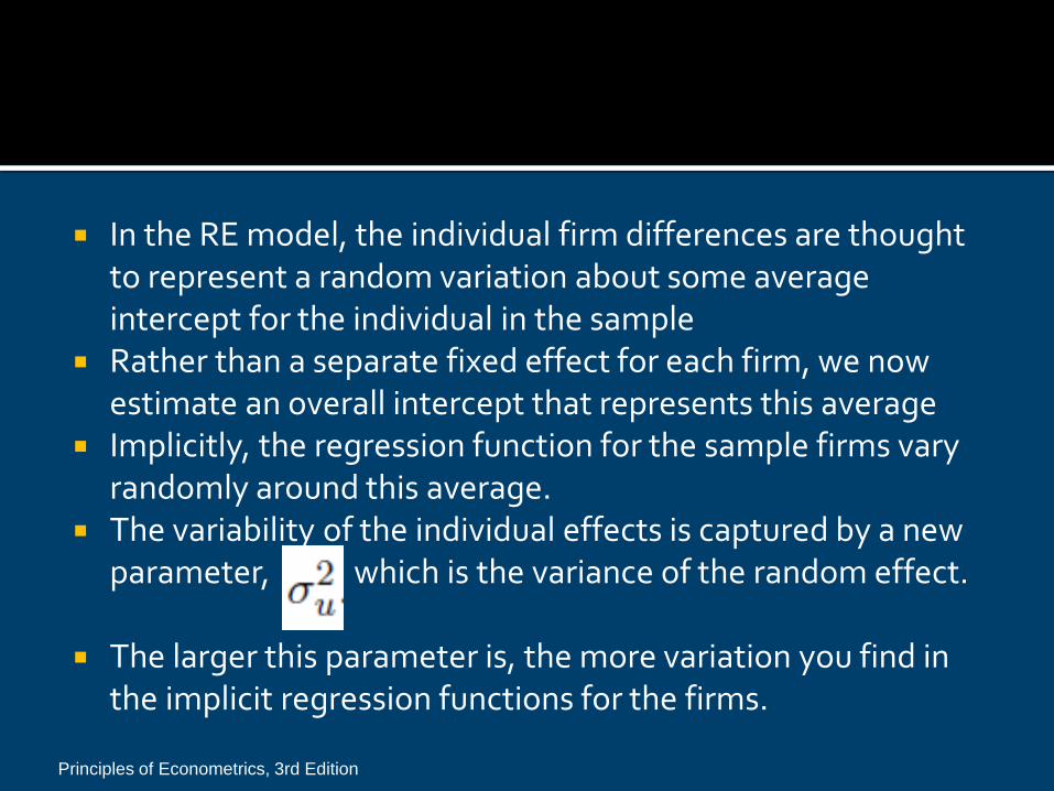
In the RE model, the individual firm differences are thought to represent a random variation about some average intercept for the individual in the sample
Rather than a separate fixed effect for each firm, we now estimate an overall intercept that represents this average
Implicitly, the regression function for the sample firms vary randomly around this average.
The variability of the individual effects is captured by a new parameter, which is the variance of the random effect.
The larger this parameter is, the more variation you find in the implicit regression functions for the firms.
Principles of Econometrics, 3rd Edition
Slide 15-38 Principles of Econometrics, 3rd Edition
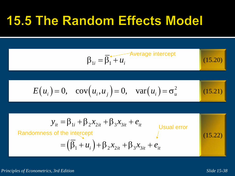
(15.20)
(15.22)
1 1i iuβ = β +
(15.21) ( ) ( ) ( ) 20, cov , 0, vari i j i uE u u u u= = = σ
( )
1 2 2 3 3
1 2 2 3 3
it i it it it
i it it it
y x x e
u x x e
= β +β +β +
= β + +β +β +Randomness of the intercept
Usual error
Average intercept
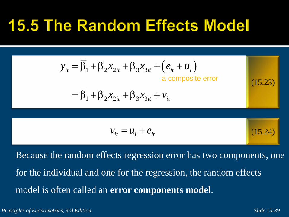
Because the random effects regression error has two components, one
for the individual and one for the regression, the random effects
model is often called an error components model.
Slide 15-39 Principles of Econometrics, 3rd Edition
(15.23)
(15.24)
( )1 2 2 3 3
1 2 2 3 3
it it it it i
it it it
y x x e u
x x v
= β +β +β + +
= β +β +β +
it i itv u e= +
a composite error
Slide 15-40 Principles of Econometrics, 3rd Edition
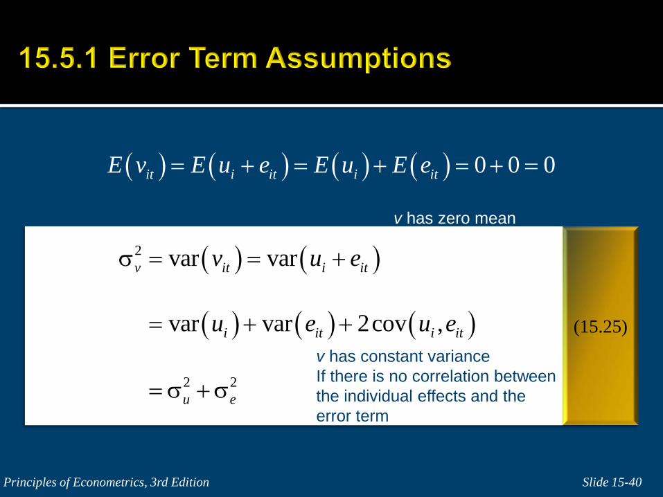
(15.25)
( ) ( ) ( ) ( ) 0 0 0it i it i itE v E u e E u E e= + = + = + =
( ) ( )
( ) ( ) ( )
2
2 2
var var
var var 2cov ,
v it i it
i it i it
u e
v u e
u e u e
σ = = +
= + +
= σ +σ
v has zero mean
v has constant variance If there is no correlation between the individual effects and the error term
Slide 15-41 Principles of Econometrics, 3rd Edition
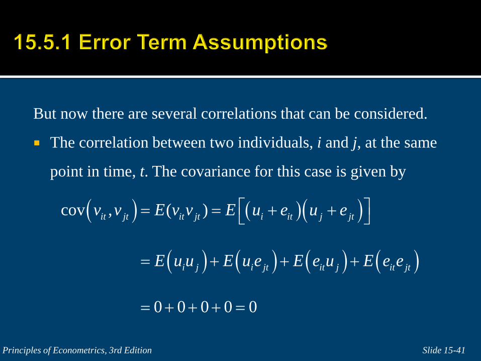
But now there are several correlations that can be considered.
The correlation between two individuals, i and j, at the same
point in time, t. The covariance for this case is given by
( ) ( )( )
( ) ( ) ( ) ( )
cov , ( )
0 0 0 0 0
it jt it jt i it j jt
i j i jt it j it jt
v v E v v E u e u e
E u u E u e E e u E e e
= = + +
= + + +
= + + + =
Slide 15-42 Principles of Econometrics, 3rd Edition
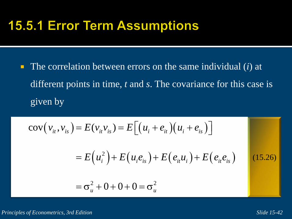
The correlation between errors on the same individual (i) at
different points in time, t and s. The covariance for this case is
given by
(15.26)
( ) ( )( )
( ) ( ) ( ) ( )2
2 2
cov , ( )
0 0 0
it is it is i it i is
i i is it i it is
u u
v v E v v E u e u e
E u E u e E e u E e e
= = + +
= + + +
= σ + + + = σ
Slide 15-43 Principles of Econometrics, 3rd Edition
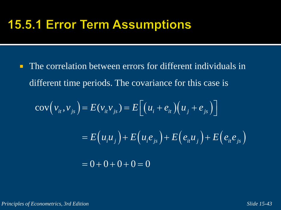
The correlation between errors for different individuals in
different time periods. The covariance for this case is
( ) ( )( )
( ) ( ) ( ) ( )
cov , ( )
0 0 0 0 0
it js it js i it j js
i j i js it j it js
v v E v v E u e u e
E u u E u e E e u E e e
= = + +
= + + +
= + + + =
Slide 15-44 Principles of Econometrics, 3rd Edition
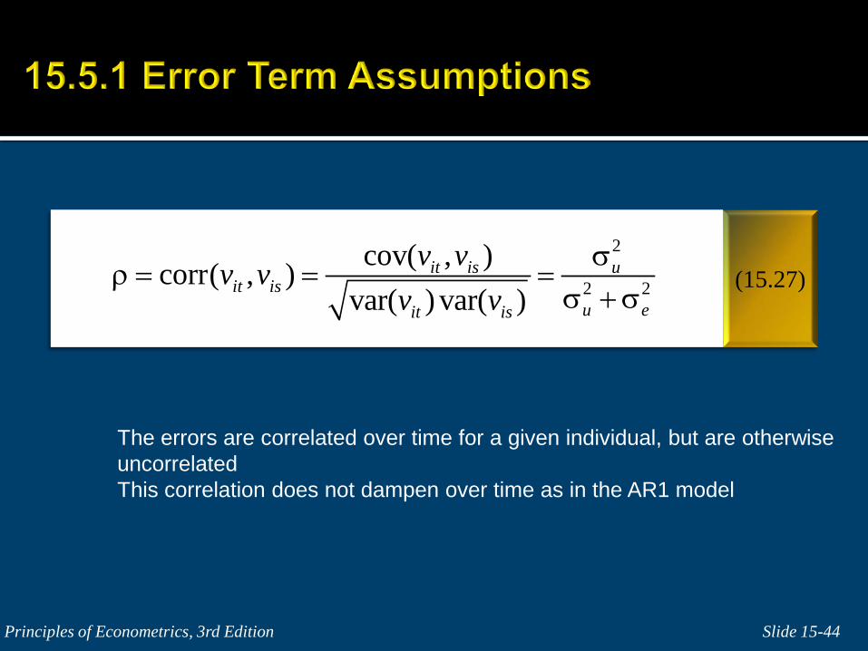
(15.27) 2
2 2cov( , )corr( , )
var( ) var( )it is u
it isu eit is
v vv vv v
σρ = = =
σ +σ
The errors are correlated over time for a given individual, but are otherwise uncorrelated This correlation does not dampen over time as in the AR1 model
Slide 15-45 Principles of Econometrics, 3rd Edition
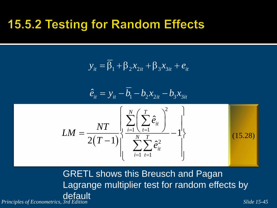
(15.28)
1 2 2 3 3it it it ity x x e= β +β +β +
1 2 2 3 3it it it ite y b b x b x= − − −
( )
2
1 1
2
1 1
ˆ1
2 1 ˆ
N T
iti t
N T
iti t
eNTLMT e
= =
= =
= − −
∑ ∑
∑∑
GRETL shows this Breusch and Pagan Lagrange multiplier test for random effects by default
Principles of Econometrics, 3rd Edition
GRETL shows by default this Breusch and Pagan Lagrangian multiplier test for RE with the null of no variation about a mean (effects are fixed) in the individual effects.
This is xttest0 in Stata…
If H0 is not rejected you can use pooled OLS if the effects are common and the FE if they differ by group

Principles of Econometrics, 3rd Edition
GRETL shows by default this Breusch and Pagan Lagrangian multiplier test for RE with the null of no variation about a mean (effects are fixed) in the individual effects.
Principles of Econometrics, 3rd Edition
GRETL also shows the Hausman test of the null hypothesis that the random effects are indeed random.
If they are random, then they should not be correlated with any of your other regressors.
If they are correlated with other regressors, then you should use the FE estimator to obtain consistent parameter estimates of your slopes
Slide 15-49 Principles of Econometrics, 3rd Edition
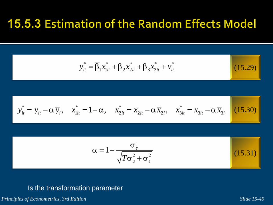
(15.29)
(15.30)
* * * * *1 1 2 2 3 3it it it it ity x x x v= β +β +β +
* * * *1 2 2 2 3 3 3, 1 , ,it it i it it it i it it iy y y x x x x x x x= −α = −α = −α = −α
(15.31) 2 21 e
u eTσ
α = −σ +σ
Is the transformation parameter
Slide 15-50 Principles of Econometrics, 3rd Edition
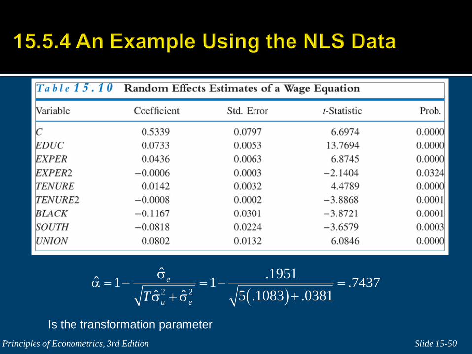
( )2 2
ˆ .1951ˆ 1 1 .74375 .1083 .0381ˆ ˆ
e
u eTσ
α = − = − =+σ +σ
Is the transformation parameter
There are different ways to calculate FE (some packages will calculate an intercept, some won’t)
There are different ways to calculate sigma-sq (STATA in textbook and GRETL will give you slightly different results!)
Principles of Econometrics, 3rd Edition
Pooled OLS vs different intercepts: test (use a Chow type, after FE or run RE and test if the variance of the intercept component of the error is zero (Breusch-Pagan test (xttest0 in STATA))
You cannot pool onto OLS? Then…
Choose between FE vs RE: (Hausman test)
GRETL summary tests: panel Inv const V K --pooled
Different slopes too perhaps? => use SURE or RCM and test for equality of slopes across units
Note that there is within variation versus between variation
The OLS is an unweighted average of the between estimator and the within estimator
The RE is a weighted average of the between estimator and the within estimator
The FE is also a weighted average of the between estimator and the within estimator with zero as the weight for the between part
The RE is a weighted average of the between
estimator and the within estimator The FE is also a weighted average of the
between estimator and the within estimator with zero as the weight for the between part
So now you see where the extra efficiency of RE comes from!...
The RE uses information from both the cross-
sectional variation in the panel and the time series variation, so it mixes LR and SR effects
The FE uses only information from the time series variation, so it estimates SR* effects
With a panel, we can learn about dynamic
effects from a short panel, while we need a long time series on a single cross-sectional unit, to learn about dynamics from a time series data set
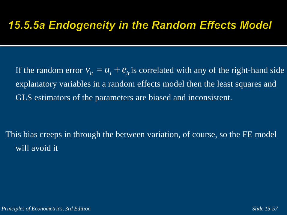
If the random error is correlated with any of the right-hand side explanatory variables in a random effects model then the least squares and GLS estimators of the parameters are biased and inconsistent.
This bias creeps in through the between variation, of course, so the FE model will avoid it
Slide 15-57 Principles of Econometrics, 3rd Edition
it i itv u e= +
Slide 15-58 Principles of Econometrics, 3rd Edition
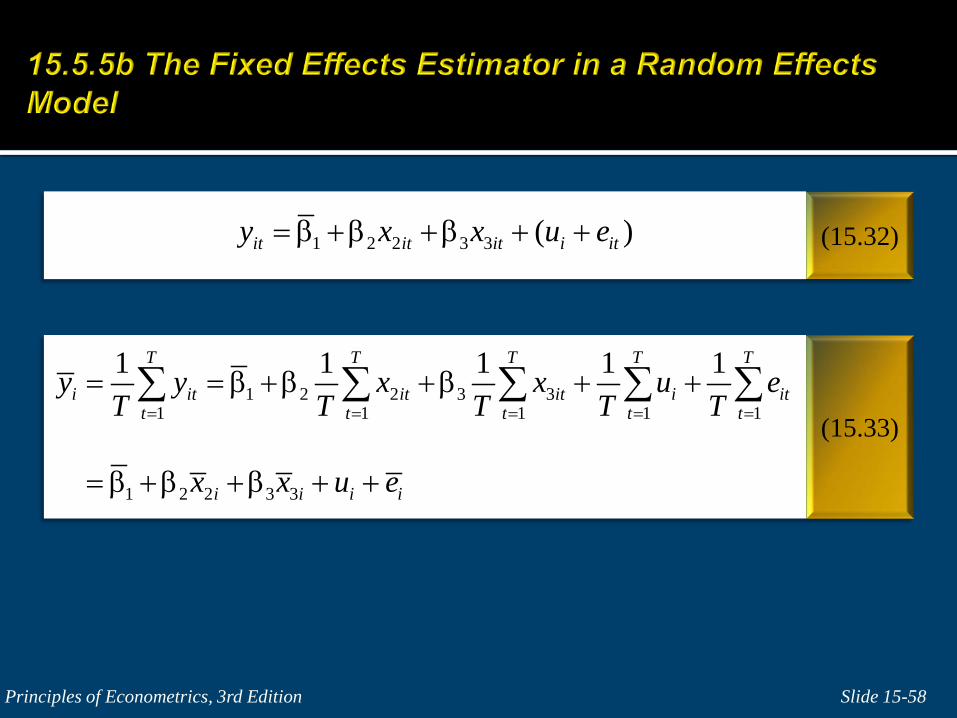
(15.32)
(15.33) 1 2 2 3 3
1 1 1 1 1
1 2 2 3 3
1 1 1 1 1T T T T T
i it it it i itt t t t t
i i i i
y y x x u eT T T T T
x x u e
= = = = == = β +β +β + +
= β +β +β + +
∑ ∑ ∑ ∑ ∑
1 2 2 3 3 ( )it it it i ity x x u e= β +β +β + +
Slide 15-59 Principles of Econometrics, 3rd Edition
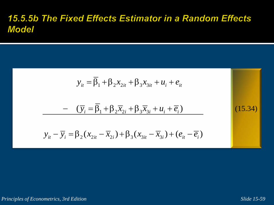
(15.34)
1 2 2 3 3
1 2 2 3 3
2 2 2 3 3 3
( )
( ) ( ) ( )
it it it i it
i i i i i
it i it i it i it i
y x x u e
y x x u e
y y x x x x e e
= β +β +β + +
− = β +β +β + +
− = β − +β − + −
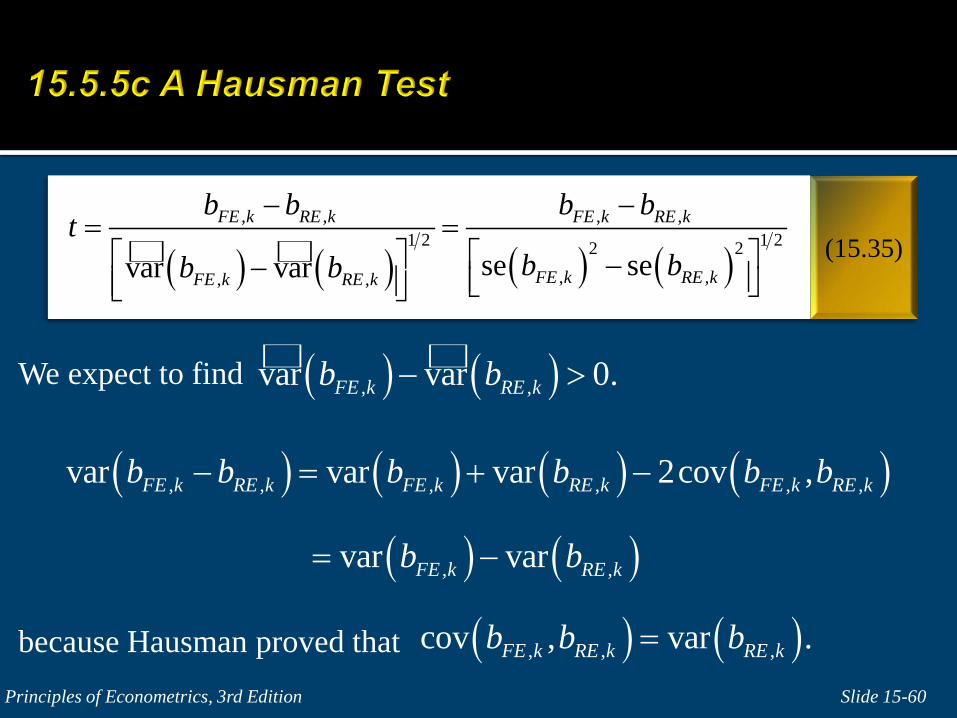
We expect to find because Hausman proved that
Slide 15-60 Principles of Econometrics, 3rd Edition
(15.35) ( ) ( ) ( ) ( ), , , ,
1 2 1 22 2, ,, , se sevar var
FE k RE k FE k RE k
FE k RE kFE k RE k
b b b bt
b bb b
− −= = −−
( ) ( ), ,var var 0.FE k RE kb b− >
( ) ( ) ( ) ( )
( ) ( )
, , , , , ,
, ,
var var var 2cov ,
var var
FE k RE k FE k RE k FE k RE k
FE k RE k
b b b b b b
b b
− = + −
= −
( ) ( ), , ,cov , var .FE k RE k RE kb b b=
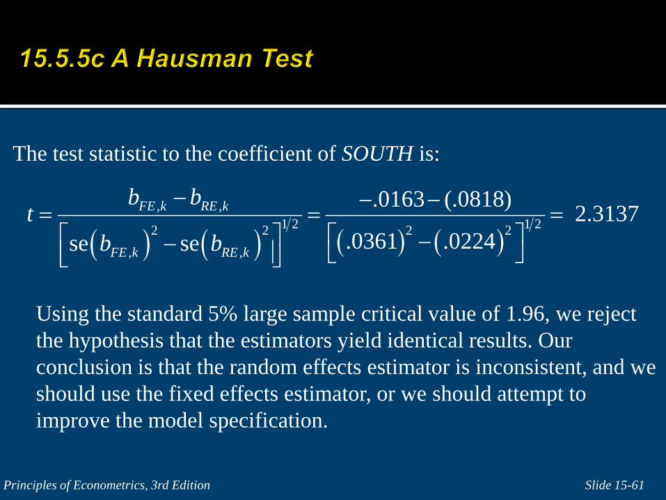
The test statistic to the coefficient of SOUTH is: Using the standard 5% large sample critical value of 1.96, we reject
the hypothesis that the estimators yield identical results. Our conclusion is that the random effects estimator is inconsistent, and we should use the fixed effects estimator, or we should attempt to improve the model specification.
Slide 15-61 Principles of Econometrics, 3rd Edition
( ) ( ) ( ) ( ), ,
1 2 1 22 2 2 2, ,
.0163 (.0818) 2.3137.0361 .0224se se
FE k RE k
FE k RE k
b bt
b b
− − −= = = −−
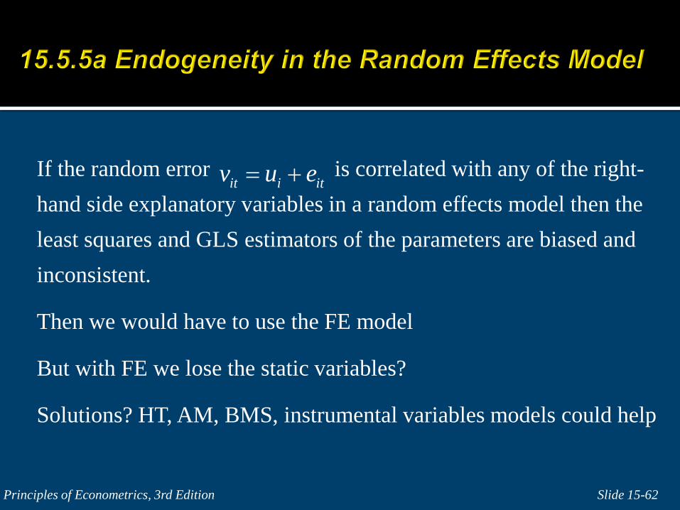
If the random error is correlated with any of the right-hand side explanatory variables in a random effects model then the least squares and GLS estimators of the parameters are biased and inconsistent.
Then we would have to use the FE model
But with FE we lose the static variables?
Solutions? HT, AM, BMS, instrumental variables models could help
Slide 15-62 Principles of Econometrics, 3rd Edition
it i itv u e= +
We can generalise the random effects idea and allow for different
slopes too: Random Coefficients Model
Again, the now it is the slope parameters that differ, but as in RE
model, they are drawn from a common distribution
The RCM in a way is to the RE model what the SURE model is to the
FE model
Slide 15-63 Principles of Econometrics, 3rd Edition
Further issues
Unit root tests and Cointegration in panels
Dynamics in panels
Slide 15-64 Principles of Econometrics, 3rd Edition
Further issues
Of course it is not necessary that one of the dimensions of the panel is time
as such Example: i are students and t is for each quiz they take
Of course we could have a one-way effect model on the time dimension
instead
Or a two-way model
Or a three way model! But things get a bit more complicated there…
Slide 15-65 Principles of Econometrics, 3rd Edition
Further issues
Another way to have more fun with panel data is to consider dependent variables that are not continuous
Logit, probit, count data can be considered
STATA has commands for these
Based on maximum likelihood and other estimation techniques we have not yet considered
Slide 15-66 Principles of Econometrics, 3rd Edition
Further issues
You can understand the use of the FE model as a solution to omitted variable bias
If the unmeasured variables left in the error model are not correlated
with the ones in the model, we would not have a bias in OLS, so we
can safely use RE
If the unmeasured variables left in the error model are correlated with
the ones in the model, we would have a bias in OLS, so we cannot
use RE, we should not leave them out and we should use FE, which
bundles them together in each cross-sectional dummy
Slide 15-67 Principles of Econometrics, 3rd Edition
Further issues
Another criterion to choose between FE and RE
If the panel include all the relevant cross-sectional units, use FE, if only a random sample from a population, RE is more appropriate (as long as it is valid)
Slide 15-68 Principles of Econometrics, 3rd Edition
Further issues
Wooldridge’s book on panel data
Baltagi’s book on panel data
Greene’s coverage is also good
Slide 15-69 Principles of Econometrics, 3rd Edition
Readings
Slide 15-70 Principles of Econometrics, 3rd Edition
Balanced panel Breusch-Pagan test Cluster corrected standard errors Contemporaneous correlation Endogeneity Error components model Fixed effects estimator Fixed effects model Hausman test Heterogeneity Least squares dummy variable
model LM test Panel corrected standard errors Pooled panel data regression
Pooled regression Random effects estimator Random effects model Seemingly unrelated regressions Unbalanced panel
Slide 15-71 Principles of Econometrics, 3rd Edition
Principles of Econometrics, 3rd Edition Slide 15-72
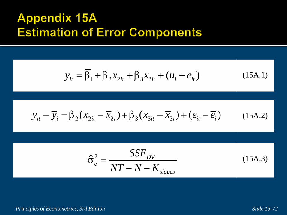
(15A.1)
(15A.2)
(15A.3)
1 2 2 3 3 ( )it it it i ity x x u e= β +β +β + +
2 2 2 3 3 3( ) ( ) ( )it i it i it i it iy y x x x x e e− = β − +β − + −
2ˆ DVe
slopes
SSENT N K
σ =− −
Principles of Econometrics, 3rd Edition Slide 15-73
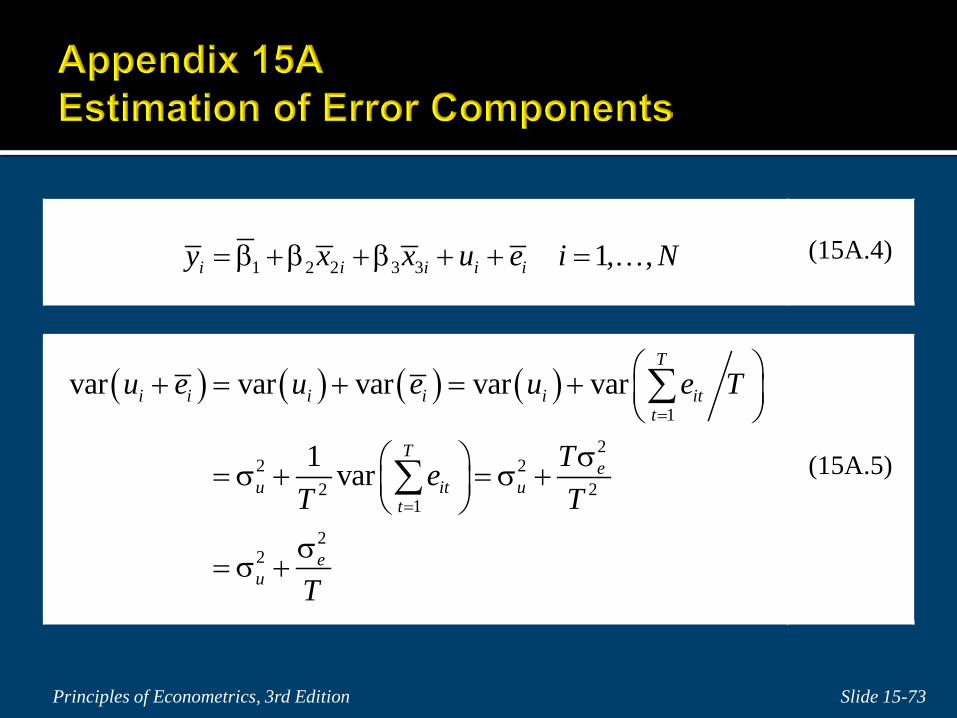
(15A.4)
(15A.5)
1 2 2 3 3 1, ,i i i i iy x x u e i N= β +β +β + + =
( ) ( ) ( ) ( )1
22 2
2 21
22
var var var var var
1 var
T
i i i i i itt
Te
u it ut
eu
u e u e u e T
TeT T
T
=
=
+ = + = +
σ = σ + = σ +
σ= σ +
∑
∑
Principles of Econometrics, 3rd Edition Slide 15-74
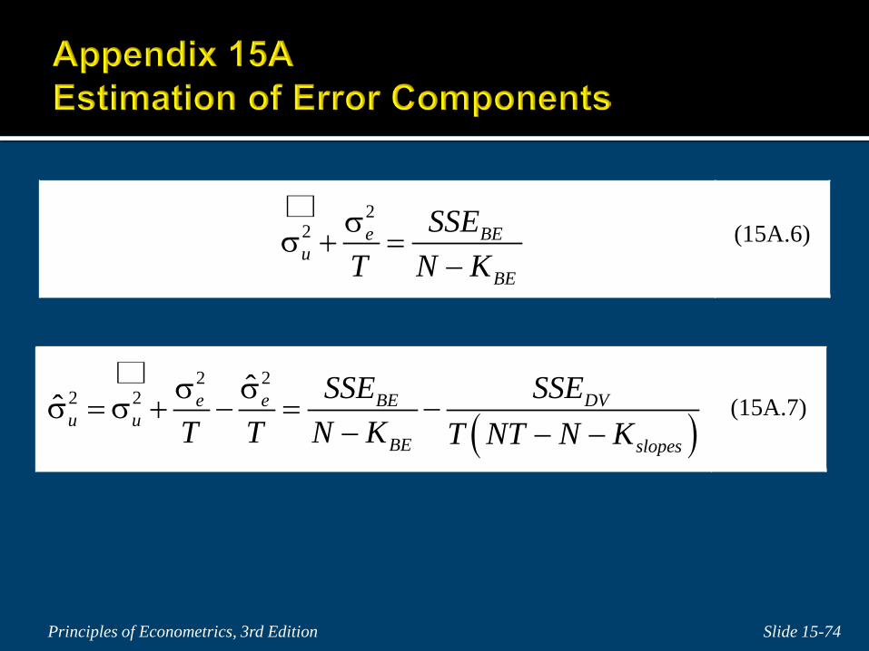
(15A.6)
(15A.7)
22 e BEu
BE
SSET N Kσ
σ + =−
( )2 2
2 2 ˆˆ e e BE DVu u
BE slopes
SSE SSET T N K T NT N Kσ σ
σ = σ + − = −− − −