Econometrics: Models with Endogenous Explanatory Variables
73
Econometrics: Models with Endogenous Explanatory Variables Burcu Eke UC3M
Transcript of Econometrics: Models with Endogenous Explanatory Variables
Econometrics:Models with Endogenous Explanatory Variables
Burcu Eke
UC3M
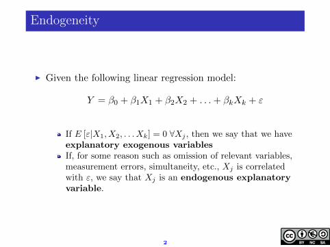
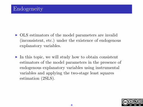
Endogeneity
I Given the following linear regression model:
Y = β0 + β1X1 + β2X2 + . . .+ βkXk + ε
If E [ε|X1, X2, . . . Xk] = 0 ∀Xj , then we say that we haveexplanatory exogenous variablesIf, for some reason such as omission of relevant variables,measurement errors, simultaneity, etc., Xj is correlatedwith ε, we say that Xj is an endogenous explanatoryvariable.
2
Endogeneity
I OLS estimators of the model parameters are invalid(inconsistent, etc.) under the existence of endogenousexplanatory variables.
I In this topic, we will study how to obtain consistentestimators of the model parameters in the presence ofendogenous explanatory variables using instrumentalvariables and applying the two-stage least squaresestimation (2SLS).
3
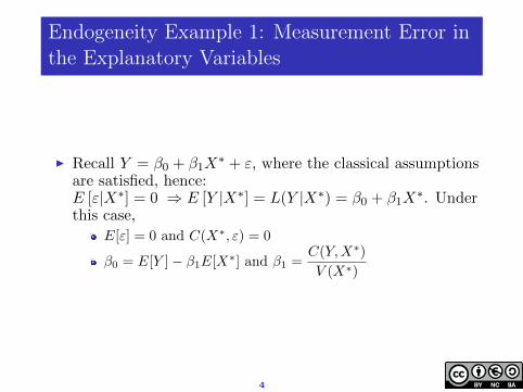
Endogeneity Example 1: Measurement Error inthe Explanatory Variables
I Recall Y = β0 + β1X∗ + ε, where the classical assumptions
are satisfied, hence:E [ε|X∗] = 0 ⇒ E [Y |X∗] = L(Y |X∗) = β0 + β1X
∗. Underthis case,
E[ε] = 0 and C(X∗, ε) = 0
β0 = E[Y ]− β1E[X∗] and β1 =C(Y,X∗)
V (X∗)
4
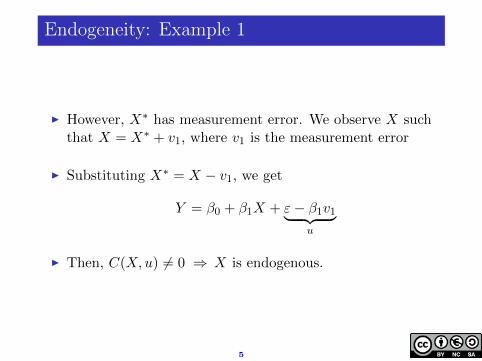
Endogeneity: Example 1
I However, X∗ has measurement error. We observe X suchthat X = X∗ + v1, where v1 is the measurement error
I Substituting X∗ = X − v1, we get
Y = β0 + β1X + ε− β1v1︸ ︷︷ ︸u
I Then, C(X,u) 6= 0 ⇒ X is endogenous.
5
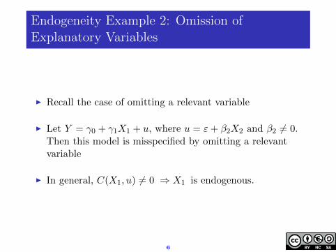
Endogeneity Example 2: Omission ofExplanatory Variables
I Recall the case of omitting a relevant variable
I Let Y = γ0 + γ1X1 + u, where u = ε+ β2X2 and β2 6= 0.Then this model is misspecified by omitting a relevantvariable
I In general, C(X1, u) 6= 0 ⇒ X1 is endogenous.
6
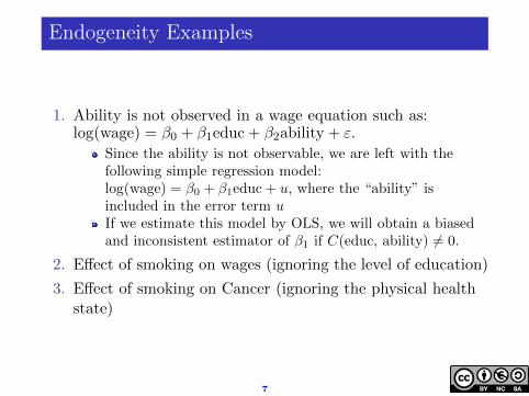
Endogeneity Examples
1. Ability is not observed in a wage equation such as:log(wage) = β0 + β1educ + β2ability + ε.
Since the ability is not observable, we are left with thefollowing simple regression model:log(wage) = β0 + β1educ + u, where the “ability” isincluded in the error term uIf we estimate this model by OLS, we will obtain a biasedand inconsistent estimator of β1 if C(educ, ability) 6= 0.
2. Effect of smoking on wages (ignoring the level of education)
3. Effect of smoking on Cancer (ignoring the physical healthstate)
7
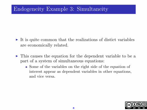
Endogeneity Example 3: Simultaneity
I It is quite common that the realizations of distict variablesare economically related.
I This causes the equation for the dependent variable to be apart of a system of simultaneous equations:
Some of the variables on the right side of the equation ofinterest appear as dependent variables in other equations,and vice versa.
8
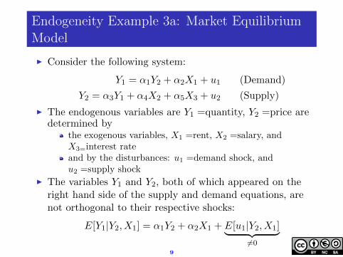
Endogeneity Example 3a: Market EquilibriumModel
I Consider the following system:
Y1 = α1Y2 + α2X1 + u1 (Demand)
Y2 = α3Y1 + α4X2 + α5X3 + u2 (Supply)
I The endogenous variables are Y1 =quantity, Y2 =price aredetermined by
the exogenous variables, X1 =rent, X2 =salary, andX3=interest rateand by the disturbances: u1 =demand shock, andu2 =supply shock
I The variables Y1 and Y2, both of which appeared on theright hand side of the supply and demand equations, arenot orthogonal to their respective shocks:
E[Y1|Y2, X1] = α1Y2 + α2X1 + E[u1|Y2, X1]︸ ︷︷ ︸6=0
9
Endogeneity Example 3b: Production Function
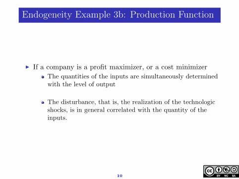
I If a company is a profit maximizer, or a cost minimizer
The quantities of the inputs are simultaneously determinedwith the level of output
The disturbance, that is, the realization of the technologicshocks, is in general correlated with the quantity of theinputs.
10

Instrumental Variables
I Instrumental variables (IV) approach allows us to getconsistent estimators of the population parameters whenthe OLS estimators are inconsistent (in situations such asomitting a relevant variable, measurement errors, andsimultaneity)
11
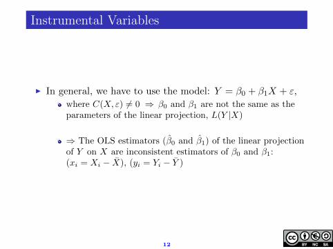
Instrumental Variables
I In general, we have to use the model: Y = β0 + β1X + ε,
where C(X, ε) 6= 0 ⇒ β0 and β1 are not the same as theparameters of the linear projection, L(Y |X)
⇒ The OLS estimators (β0 and β1) of the linear projectionof Y on X are inconsistent estimators of β0 and β1:(xi = Xi − X), (yi = Yi − Y )
12
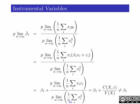
Instrumental Variables
p limn→∞
β1 =
p limn→∞
(1
n
∑i
xiyi
)
p limn→∞
(1
n
∑i
x2i
)
=
p limn→∞
(1
n
∑i
xi(β1xi + εi)
)
p limn→∞
(1
n
∑i
x2i
)
= β1 +
p limn→∞
(1
n
∑i
xiεi
)
p limn→∞
(1
n
∑i
x2i
) = β1 +C(X, ε)
V (X)6= β1
13
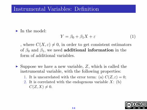
Instrumental Variables: Definition
I In the model:Y = β0 + β1X + ε (1)
, where C(X, ε) 6= 0, in order to get consistent estimatorsof β0 and β1, we need additional information in theform of additional variables.
I Suppose we have a new variable, Z, which is called theinstrumental variable, with the following properties:
1. It is uncorrelated with the error term: (a) C(Z, ε) = 0;2. It is correlated with the endogenous variable X: (b)
C(Z,X) 6= 0.
14
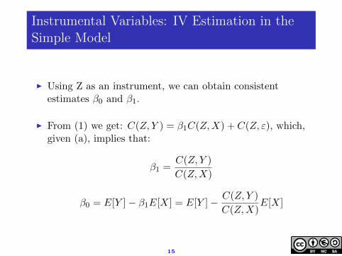
Instrumental Variables: IV Estimation in theSimple Model
I Using Z as an instrument, we can obtain consistentestimates β0 and β1.
I From (1) we get: C(Z, Y ) = β1C(Z,X) + C(Z, ε), which,given (a), implies that:
β1 =C(Z, Y )
C(Z,X)
β0 = E[Y ]− β1E[X] = E[Y ]− C(Z, Y )
C(Z,X)E[X]
15
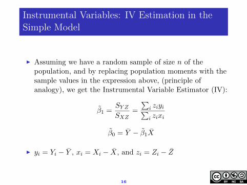
Instrumental Variables: IV Estimation in theSimple Model
I Assuming we have a random sample of size n of thepopulation, and by replacing population moments with thesample values in the expression above, (principle ofanalogy), we get the Instrumental Variable Estimator (IV):
β1 =SY ZSXZ
=
∑i ziyi∑i zixi
β0 = Y − β1X
I yi = Yi − Y , xi = Xi − X, and zi = Zi − Z
16
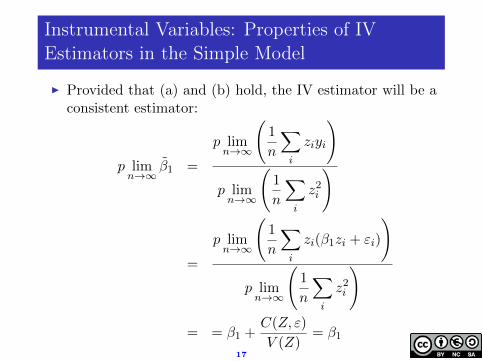
Instrumental Variables: Properties of IVEstimators in the Simple Model
I Provided that (a) and (b) hold, the IV estimator will be aconsistent estimator:
p limn→∞
β1 =
p limn→∞
(1
n
∑i
ziyi
)
p limn→∞
(1
n
∑i
z2i
)
=
p limn→∞
(1
n
∑i
zi(β1zi + εi)
)
p limn→∞
(1
n
∑i
z2i
)
= = β1 +C(Z, ε)
V (Z)= β1
17
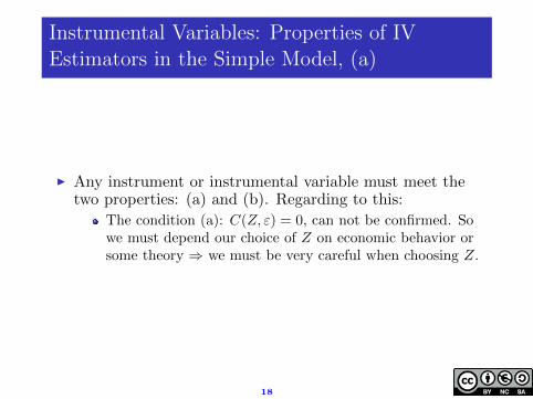
Instrumental Variables: Properties of IVEstimators in the Simple Model, (a)
I Any instrument or instrumental variable must meet thetwo properties: (a) and (b). Regarding to this:
The condition (a): C(Z, ε) = 0, can not be confirmed. Sowe must depend our choice of Z on economic behavior orsome theory ⇒ we must be very careful when choosing Z.
18
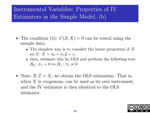
Instrumental Variables: Properties of IVEstimators in the Simple Model, (b)
I The condition (b): C(Z,X) = 0 can be tested using thesample data.
The simplest way is to consider the linear projection of Xon Z: X = π0 + π1Z + v,then, estimate this by OLS and perform the following test:H0 : π1 = 0 vs H1 : π1 6= 0
I Note: If Z = X, we obtain the OLS estimation. That is,when X is exogenous, can be used as its own instrument,and the IV estimator is then identical to the OLSestimator.
19

Instrumental Variables: The Variance of the IVEstimator
I In general, the IV estimator will have a larger variancethan the OLS estimator.
I To see this, let’s drive the estimated variance of the IVestimator β1, S
2β1
:
S2β1≡ V
(β1
)=σ2S2
Z
nS2ZX
=σ2
nr2ZXS2X
where rZX =SZXSZSX
, is the sample correlation coefficient
between X and Z, which measures the degree of linearrelationship between X and Z in the sample.
20
Instrumental Variables: The Variance of the IVEstimator
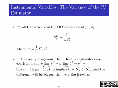
I Recall the variance of the OLS estimator of β1, β1:
S2β1
=σ2
nS2X
where σ2 =1
n
∑i ε
2i
I If X is really exogenous, then, the OLS estimators areconsistent, and p lim
n→∞σ2 = p lim
n→∞σ2 = σ2 =
Since 0 < |rZX | < 1, this implies that S2β1> S2
β1, and the
difference will be bigger, the lower the |rZX | is.
21
Instrumental Variables: The Variance of the IVEstimator
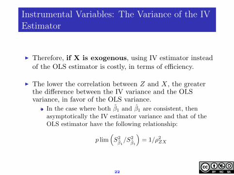
I Therefore, if X is exogenous, using IV estimator insteadof the OLS estimator is costly, in terms of efficiency.
I The lower the correlation between Z and X, the greaterthe difference between the IV variance and the OLSvariance, in favor of the OLS variance.
In the case where both β1 and β1 are consistent, thenasymptotically the IV estimator variance and that of theOLS estimator have the following relationship:
p lim(S2β1/S2
β1
)= 1/ρ2ZX
22
Instrumental Variables: The Variance of the IVEstimator
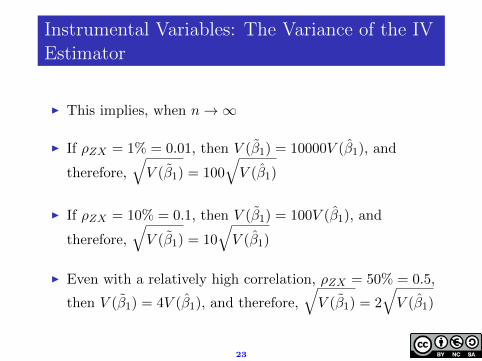
I This implies, when n→∞
I If ρZX = 1% = 0.01, then V (β1) = 10000V (β1), and
therefore,√V (β1) = 100
√V (β1)
I If ρZX = 10% = 0.1, then V (β1) = 100V (β1), and
therefore,√V (β1) = 10
√V (β1)
I Even with a relatively high correlation, ρZX = 50% = 0.5,
then V (β1) = 4V (β1), and therefore,√V (β1) = 2
√V (β1)
23
Instrumental Variables: The Variance of the IVEstimator
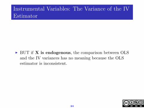
I BUT if X is endogenous, the comparison between OLSand the IV variances has no meaning because the OLSestimator is inconsistent.
24
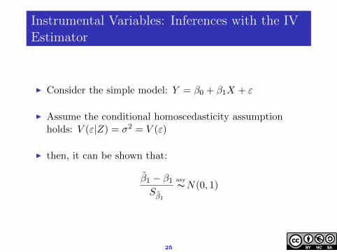
Instrumental Variables: Inferences with the IVEstimator
I Consider the simple model: Y = β0 + β1X + ε
I Assume the conditional homoscedasticity assumptionholds: V (ε|Z) = σ2 = V (ε)
I then, it can be shown that:
β1 − β1Sβ1
∼asyN(0, 1)
25

Instrumental Variables: Inferences with the IVEstimator
I Sβ1 is the standard error of the IV estimators:
S2β1≡ V
(β1
)=σ2S2
Z
nS2ZX
⇒ Sβ1 =σ√nSZX
I where σ2 =1
n
∑i ε
2i , and εi = Yi −
(β0 + β1X
)= yi − β1xi
I This result allows us to construct confidence intervals, andperform hypothesis tests.
26
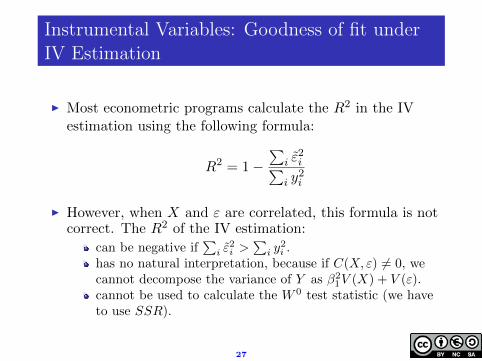
Instrumental Variables: Goodness of fit underIV Estimation
I Most econometric programs calculate the R2 in the IVestimation using the following formula:
R2 = 1−∑
i ε2i∑
i y2i
I However, when X and ε are correlated, this formula is notcorrect. The R2 of the IV estimation:
can be negative if∑i ε
2i >
∑i y
2i .
has no natural interpretation, because if C(X, ε) 6= 0, wecannot decompose the variance of Y as β2
1V (X) + V (ε).cannot be used to calculate the W 0 test statistic (we haveto use SSR).
27
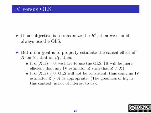
IV versus OLS
I If our objective is to maximize the R2, then we shouldalways use the OLS.
I But if our goal is to properly estimate the causal effect ofX on Y , that is, β1, then:
If C(X, ε) = 0, we have to use the OLS. (It will be moreefficient than any IV estimator Z such that Z 6= X).If C(X, ε) 6= 0, OLS will not be consistent, thus using an IVestimator Z 6= X is appropriate. (The goodness of fit, inthis context, is not of interest to us).
28
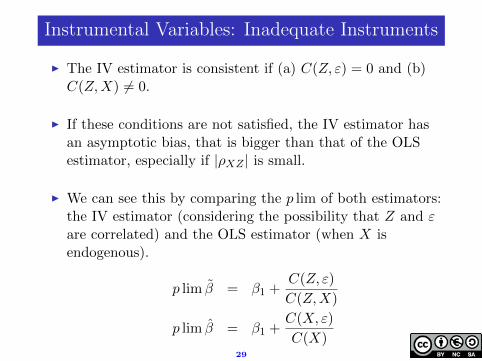
Instrumental Variables: Inadequate Instruments
I The IV estimator is consistent if (a) C(Z, ε) = 0 and (b)C(Z,X) 6= 0.
I If these conditions are not satisfied, the IV estimator hasan asymptotic bias, that is bigger than that of the OLSestimator, especially if |ρXZ | is small.
I We can see this by comparing the p lim of both estimators:the IV estimator (considering the possibility that Z and εare correlated) and the OLS estimator (when X isendogenous).
p lim β = β1 +C(Z, ε)
C(Z,X)
p lim β = β1 +C(X, ε)
C(X)29
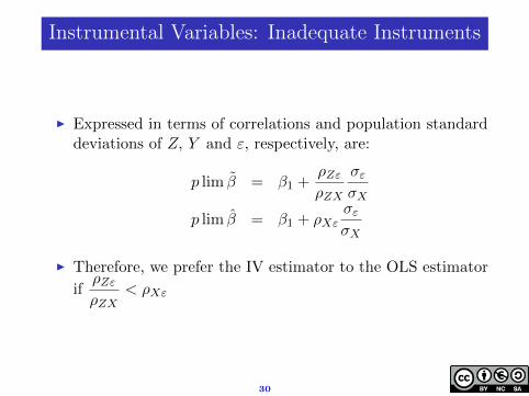
Instrumental Variables: Inadequate Instruments
I Expressed in terms of correlations and population standarddeviations of Z, Y and ε, respectively, are:
p lim β = β1 +ρZερZX
σεσX
p lim β = β1 + ρXεσεσX
I Therefore, we prefer the IV estimator to the OLS estimator
ifρZερZX
< ρXε
30
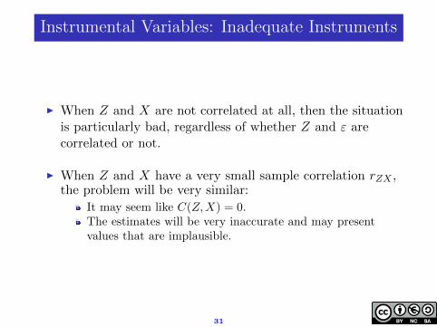
Instrumental Variables: Inadequate Instruments
I When Z and X are not correlated at all, then the situationis particularly bad, regardless of whether Z and ε arecorrelated or not.
I When Z and X have a very small sample correlation rZX ,the problem will be very similar:
It may seem like C(Z,X) = 0.The estimates will be very inaccurate and may presentvalues that are implausible.
31
Instrumental Variables: Example of InadequateInstruments
I Example: Effect of the Mother’s cigarette consumption onthe birth weight of the baby:
Following example illustrates why we should always checkwhether the endogenous explanatory variable is correlatedwith the potential instrument.Our estimation results for the effect of several variables onthe birth weight, including cigarette consumption of themother are presented below:
32
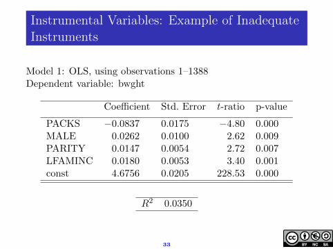
Instrumental Variables: Example of InadequateInstruments
Model 1: OLS, using observations 1–1388Dependent variable: bwght
Coefficient Std. Error t-ratio p-value
PACKS −0.0837 0.0175 −4.80 0.000MALE 0.0262 0.0100 2.62 0.009PARITY 0.0147 0.0054 2.72 0.007LFAMINC 0.0180 0.0053 3.40 0.001const 4.6756 0.0205 228.53 0.000
R2 0.0350
33
Instrumental Variables: Example of InadequateInstruments
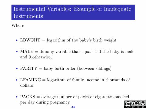
Where
I LBWGHT = logarithm of the baby’s birth weight
I MALE = dummy variable that equals 1 if the baby is maleand 0 otherwise,
I PARITY = baby birth order (between siblings)
I LFAMINC = logarithm of family income in thousands ofdollars
I PACKS = average number of packs of cigarettes smokedper day during pregnancy.
34
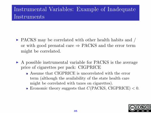
Instrumental Variables: Example of InadequateInstruments
I PACKS may be correlated with other health habits and /or with good prenatal care ⇒ PACKS and the error termmight be correlated.
I A possible instrumental variable for PACKS is the averageprice of cigarettes per pack: CIGPRICE
Assume that CIGPRICE is uncorrelated with the errorterm (although the availability of the state health caremight be correlated with taxes on cigarettes).Economic theory suggests that C(PACKS, CIGPRICE) < 0.
35
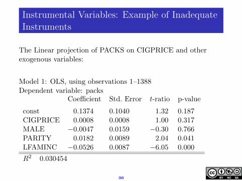
Instrumental Variables: Example of InadequateInstruments
The Linear projection of PACKS on CIGPRICE and otherexogenous variables:
Model 1: OLS, using observations 1–1388Dependent variable: packs
Coefficient Std. Error t-ratio p-value
const 0.1374 0.1040 1.32 0.187CIGPRICE 0.0008 0.0008 1.00 0.317MALE −0.0047 0.0159 −0.30 0.766PARITY 0.0182 0.0089 2.04 0.041LFAMINC −0.0526 0.0087 −6.05 0.000
R2 0.030454
36
Instrumental Variables: Example of InadequateInstruments
I The reduced form results indicate that there is norelationship between smoking during pregnancy and theprice of cigarettes (that is, the price elasticity of cigaretteconsumption, which is an addictive good, is notstatistically different from zero).
I Since CIGPRICE and PACKS and are not correlated,CIGPRICE does not satisfy the condition (b) ⇒CIGPRICE should not be used as an IV.
I But what happens if we use CIGPRICE as an instrument?The IV estimation results are:
37
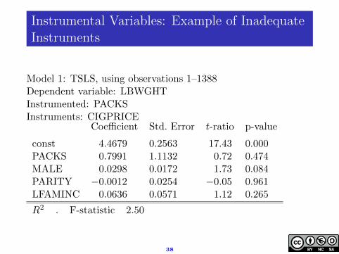
Instrumental Variables: Example of InadequateInstruments
Model 1: TSLS, using observations 1–1388Dependent variable: LBWGHTInstrumented: PACKSInstruments: CIGPRICE
Coefficient Std. Error t-ratio p-value
const 4.4679 0.2563 17.43 0.000PACKS 0.7991 1.1132 0.72 0.474MALE 0.0298 0.0172 1.73 0.084PARITY −0.0012 0.0254 −0.05 0.961LFAMINC 0.0636 0.0571 1.12 0.265
R2 . F-statistic 2.50
38
Instrumental Variables: Example of InadequateInstruments
I The coefficient of the variable PACKS is very large and ithas an opposite sign compared to what is expected. Itsstandard error is also very large.
I But these estimates are meaningless since CIGPRICE doesnot satisfy one of the requirements for a valid instrumentalvariable.
39
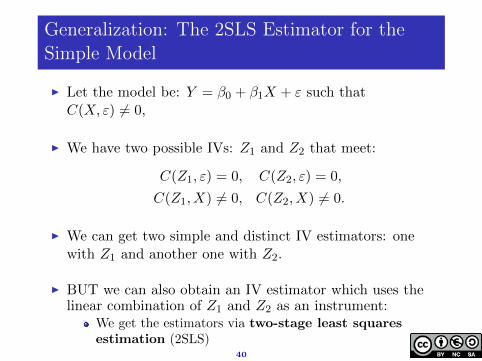
Generalization: The 2SLS Estimator for theSimple Model
I Let the model be: Y = β0 + β1X + ε such thatC(X, ε) 6= 0,
I We have two possible IVs: Z1 and Z2 that meet:
C(Z1, ε) = 0, C(Z2, ε) = 0,
C(Z1, X) 6= 0, C(Z2, X) 6= 0.
I We can get two simple and distinct IV estimators: onewith Z1 and another one with Z2.
I BUT we can also obtain an IV estimator which uses thelinear combination of Z1 and Z2 as an instrument:
We get the estimators via two-stage least squaresestimation (2SLS)
40
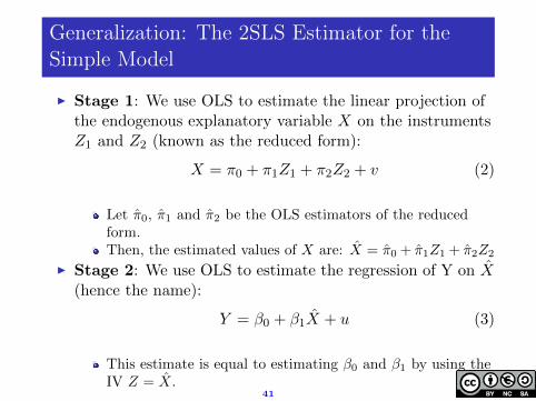
Generalization: The 2SLS Estimator for theSimple Model
I Stage 1: We use OLS to estimate the linear projection ofthe endogenous explanatory variable X on the instrumentsZ1 and Z2 (known as the reduced form):
X = π0 + π1Z1 + π2Z2 + v (2)
Let π0, π1 and π2 be the OLS estimators of the reducedform.Then, the estimated values of X are: X = π0 + π1Z1 + π2Z2
I Stage 2: We use OLS to estimate the regression of Y on X(hence the name):
Y = β0 + β1X + u (3)
This estimate is equal to estimating β0 and β1 by using theIV Z = X.
41
Generalization: The 2SLS Estimator for theSimple Model
I Although in both cases the coefficients are the same, thestandard errors obtained by 2SLS are incorrect.
The reason is that the error term of the second stage, u,includes v, but the standard error should only include thevariance of ε.
I The majority of the economic packages have special optionsfor IV estimation, which will conduct the 2SLS, so we don’tneed to perform the two stages sequentially.
42
Generalization: The 2SLS Estimator for theSimple Model
I The reduced form (2) decomposes the endogenousexplanatory variable into two additive parts:
The exogenous part, explained linearly by the instruments,π0 + π1Z1 + π2Z2
The endogenous part, the part that could not be explainedby the instruments, that is, the error term v
43
Generalization: The 2SLS Estimator,Interpretation of the Reduced Form
I If the instruments are valid and V (ε|Z1, Z2) ishomoscedastic, it can be shown that the 2SLS estimatorsare consistent and asymptomatically normal.
I Thus, we can make inferences using an estimator of thepopulation variance
σ2 =1
n
∑i
u2i
where u2i are the residuals from the 2SLS estimation.
I Similar to the simple IV estimator, when instruments arenot appropriate (because they’re correlated with the errorterm or weak correlations with the endogenous variable)the 2SLS estimators can be worse than OLS estimators.
44
Generalization: The 2SLS Estimator for theMultiple Model
I For simplicity, consider the following linear regressionmodel:
Y = β0 + β1X1 + β2X2 + ε
where E[ε] = 0, C(X1, ε) = 0, C(X2, ε) 6= 0
I That is:
X1 is an exogenous variableBut X2 is endogenous
45
Generalization: The 2SLS Estimator for theMultiple Model
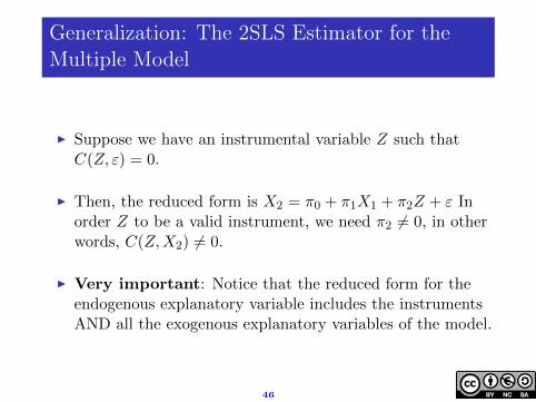
I Suppose we have an instrumental variable Z such thatC(Z, ε) = 0.
I Then, the reduced form is X2 = π0 + π1X1 + π2Z + ε Inorder Z to be a valid instrument, we need π2 6= 0, in otherwords, C(Z,X2) 6= 0.
I Very important: Notice that the reduced form for theendogenous explanatory variable includes the instrumentsAND all the exogenous explanatory variables of the model.
46

Generalization: The 2SLS Estimator for theMultiple Model
I What if we have one more endogenous variable?
I Suppose Y = β0 + β1X1 + β2X2 + β3X3 + ε, where X1 andX2 are endogenous, and X3 is exogenous.E[ε] = 0, C(X1, ε) 6= 0, C(X2, ε) 6= 0, C(X3, ε) = 0
I In that case, we will need at least as many additionalexogenous variables as endogenous explanatory variables touse as instruments.
47
Generalization: The 2SLS Estimator for theMultiple Model
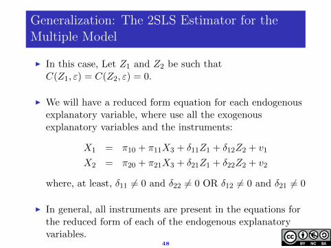
I In this case, Let Z1 and Z2 be such thatC(Z1, ε) = C(Z2, ε) = 0.
I We will have a reduced form equation for each endogenousexplanatory variable, where use all the exogenousexplanatory variables and the instruments:
X1 = π10 + π11X3 + δ11Z1 + δ12Z2 + v1
X2 = π20 + π21X3 + δ21Z1 + δ22Z2 + v2
where, at least, δ11 6= 0 and δ22 6= 0 OR δ12 6= 0 and δ21 6= 0
I In general, all instruments are present in the equations forthe reduced form of each of the endogenous explanatoryvariables.
48
Test of Endogeneity: Hausman Test
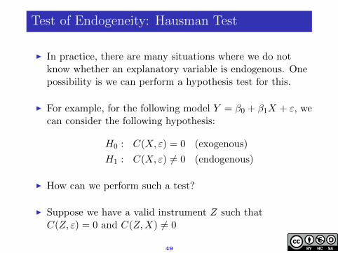
I In practice, there are many situations where we do notknow whether an explanatory variable is endogenous. Onepossibility is we can perform a hypothesis test for this.
I For example, for the following model Y = β0 + β1X + ε, wecan consider the following hypothesis:
H0 : C(X, ε) = 0 (exogenous)
H1 : C(X, ε) 6= 0 (endogenous)
I How can we perform such a test?
I Suppose we have a valid instrument Z such thatC(Z, ε) = 0 and C(Z,X) 6= 0
49
Test of Endogeneity: Hausman Test
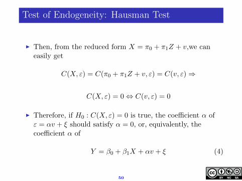
I Then, from the reduced form X = π0 + π1Z + v,we caneasily get
C(X, ε) = C(π0 + π1Z + v, ε) = C(v, ε)⇒
C(X, ε) = 0⇔ C(v, ε) = 0
I Therefore, if H0 : C(X, ε) = 0 is true, the coefficient α ofε = αv + ξ should satisfy α = 0, or, equivalently, thecoefficient α of
Y = β0 + β1X + αv + ξ (4)
50
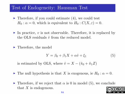
Test of Endogeneity: Hausman Test
I Therefore, if you could estimate (4), we could testH0 : α = 0, which is equivalent to H0 : C(X, ε) = 0.
I In practice, v is not observable. Therefore, it is replaced bythe OLS residuals v from the reduced model.
I Therefore, the model
Y = β0 + β1X + αv + ξ1 (5)
is estimated by OLS, where v = X − (π0 + π1Z)
I The null hypothesis is that X is exogenous, ie H0 : α = 0.
I Therefore, if we reject that α is 0 in model (5), we concludethat X is endogenous.
51
Test of Endogeneity: Hausman Test
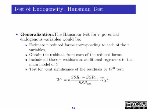
I Generalization:The Hausman test for r potentialendogenous variables would be:
Estimate r reduced forms corresponding to each of the rvariables,Obtain the residuals from each of the reduced formsInclude all these r residuals as additional regressors to themain model of YTest for joint significance of the residuals by W 0 test:
W 0 = nSSRr − SSRun
SSRun∼asy
χ2r
52
Test of Endogeneity: Hausman Test
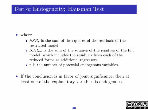
I where
SSRr is the sum of the squares of the residuals of therestricted modelSSRun is the sum of the squares of the residues of the fullmodel, which includes the residuals from each of thereduced forms as additional regressorsr is the number of potential endogenous variables.
I If the conclusion is in favor of joint significance, then atleast one of the explanatory variables is endogenous.
53
Hausman Test Example
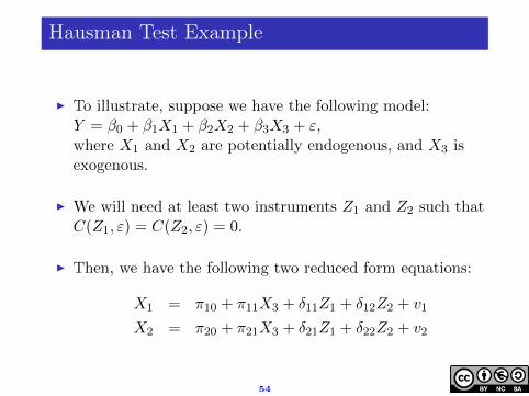
I To illustrate, suppose we have the following model:Y = β0 + β1X1 + β2X2 + β3X3 + ε,where X1 and X2 are potentially endogenous, and X3 isexogenous.
I We will need at least two instruments Z1 and Z2 such thatC(Z1, ε) = C(Z2, ε) = 0.
I Then, we have the following two reduced form equations:
X1 = π10 + π11X3 + δ11Z1 + δ12Z2 + v1
X2 = π20 + π21X3 + δ21Z1 + δ22Z2 + v2
54
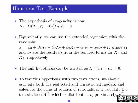
Hausman Test Example
I The hypothesis of exogeneity is nowH0 : C(X1, ε) = C(X2, ε) = 0
I Equivalently, we can use the extended regression with theresiduals:Y = β0 + β1X1 + β2X2 + β3X3 + α1v1 + α2v2 + ξ, where v1and v2 are the residuals from the reduced forms for X1 andX2, respectively
I The null hypothesis can be written as H0 : α1 = α2 = 0.
I To test this hypothesis with two restrictions, we shouldestimate both the restricted and unrestricted models, andcalculate the sums of squares of residuals, and calculate thetest statistic W 0, which is distributed, approximately, χ2
2
55
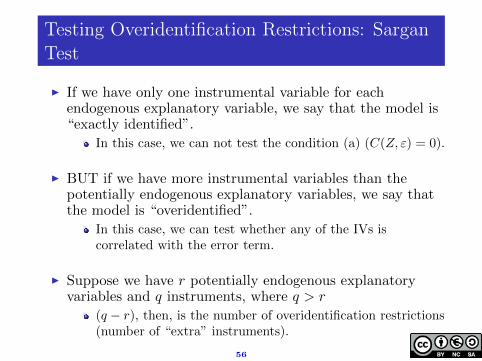
Testing Overidentification Restrictions: SarganTest
I If we have only one instrumental variable for eachendogenous explanatory variable, we say that the model is“exactly identified”.
In this case, we can not test the condition (a) (C(Z, ε) = 0).
I BUT if we have more instrumental variables than thepotentially endogenous explanatory variables, we say thatthe model is “overidentified”.
In this case, we can test whether any of the IVs iscorrelated with the error term.
I Suppose we have r potentially endogenous explanatoryvariables and q instruments, where q > r
(q − r), then, is the number of overidentification restrictions(number of “extra” instruments).
56
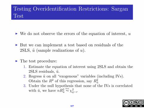
Testing Overidentification Restrictions: SarganTest
I We do not observe the errors of the equation of interest, u
I But we can implement a test based on residuals of the2SLS, u (sample realizations of u).
I The test procedure:
1. Estimate the equation of interest using 2SLS and obtain the2SLS residuals, u.
2. Regress u on all “exogenous” variables (including IVs).Obtain the R2 of this regression, say R2
u
3. Under the null hypothesis that none of the IVs is correlatedwith u, we have nR2
u ∼asyχ2q−r
57
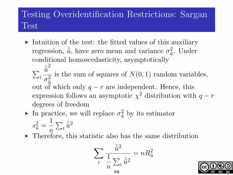
Testing Overidentification Restrictions: SarganTest
I Intuition of the test: the fitted values of this auxiliaryregression, ˆu, have zero mean and variance σ2u. Underconditional homoscedasticity, asymptotically∑
i
ˆu2
σ2uis the sum of squares of N(0, 1) random variables,
out of which only q − r are independent. Hence, thisexpression follows an asymptotic χ2 distribution with q − rdegrees of freedom
I In practice, we will replace σ2u by its estimator
s2u =1
n
∑iˆu2
I Therefore, this statistic also has the same distribution∑i
ˆu2
1
n
∑iˆu2
= nR2u
58
Testing Overidentification Restrictions: SarganTest
I If nR2u exceeds the critical value of χ2
q−r at the significancelevel, we reject H0 and conclude that there is no evidencefor exogeneity.
I Another thing is that this test does not distinguish whichvariable is the reason for rejecting the null of no correlation.
I This test is also known as Hansen-Sargan test.
59
Example: The Wage Equation
I Let the model be: ln(wage) = β0 + β1 educ + β2 cap + εwhere β2 6= 0 (ie, the variable capacity, which isunobserved, is a relevant variable).
I If we estimate the model using OLS:ln(wage) = β0 + β1educ + u, with u = β2cap + ε, we willhave inconsistent estimates.
I If we have an instrumental variable for educ, we canestimate the model by IV estimation.
60
Example: The Wage Equation
I What are the conditions for the IV in order our estimatorsto be consistent?
1. C(Z, u) = 0: IV should not be correlated with the capacityor other unobserved variables that affect wages.
2. C(Z, educ) 6= 0: IV should be correlated with education.
I Some examples of possible instruments (Z) for educationare, mother’s education, father’s education, number ofsiblings, distance between school and home, etc.
61
Example: The Wage Equation, OLS estimation
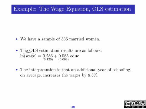
I We have a sample of 336 married women.
I The OLS estimation results are as follows:ln(wage) = 0.286
(0.120)+ 0.083
(0.009)educ
I The interpretation is that an additional year of schooling,on average, increases the wages by 8.3%.
62
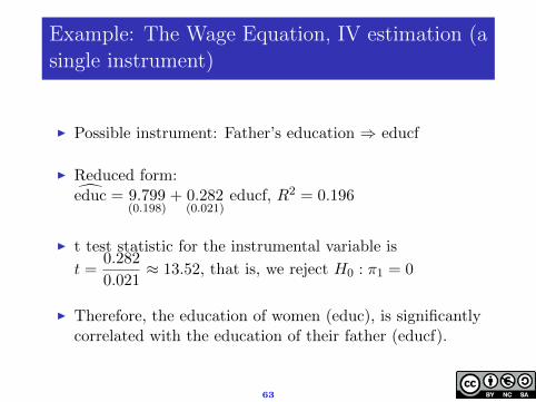
Example: The Wage Equation, IV estimation (asingle instrument)
I Possible instrument: Father’s education ⇒ educf
I Reduced form:educ = 9.799
(0.198)+ 0.282
(0.021)educf, R2 = 0.196
I t test statistic for the instrumental variable is
t =0.282
0.021≈ 13.52, that is, we reject H0 : π1 = 0
I Therefore, the education of women (educ), is significantlycorrelated with the education of their father (educf).
63

Example: The Wage Equation, IV estimation (asingle instrument)
I The IV Estimate: ln(wage) = 0.363(0.289)
+ 0.076(0.023)
educ
I By comparing the results of OLS with that of IV, we seethat the OLS estimate is higher, which is consistent with apositive bias due to omitting capacity.
I Notice that the standard error of the IV estimators aresubstantially higher than those of the OLS estimators asthe theory suggests (but education still remains significant)
64
Example: The Wage Equation, IV estimation (asingle instrument)
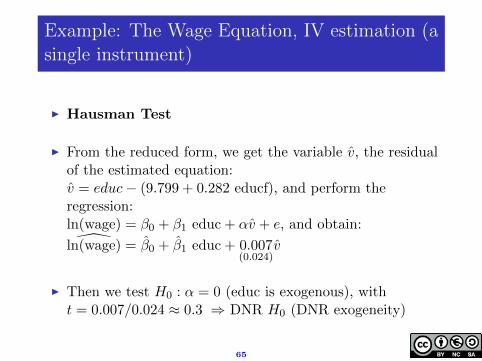
I Hausman Test
I From the reduced form, we get the variable v, the residualof the estimated equation:v = educ− (9.799 + 0.282 educf), and perform theregression:ln(wage) = β0 + β1 educ + αv + e, and obtain:ln(wage) = β0 + β1 educ + 0.007
(0.024)v
I Then we test H0 : α = 0 (educ is exogenous), witht = 0.007/0.024 ≈ 0.3 ⇒ DNR H0 (DNR exogeneity)
65
Example: The Wage Equation, IV estimation(multiple instruments)
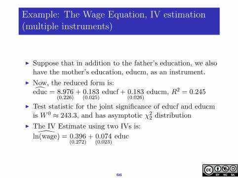
I Suppose that in addition to the father’s education, we alsohave the mother’s education, educm, as an instrument.
I Now, the reduced form is:educ = 8.976
(0.226)+ 0.183
(0.025)educf + 0.183
(0.026)educm, R2 = 0.245
I Test statistic for the joint significance of educf and educmis W 0 ≈ 243.3, and has asymptotic χ2
2 distribution
I The IV Estimate using two IVs is:ln(wage) = 0.396
(0.272)+ 0.074
(0.023)educ
66
Example: The Wage Equation, IV estimation(multiple instruments)
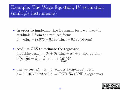
I In order to implement the Hausman test, we take theresiduals v from the reduced form:v = educ− (8.976 + 0.183 educf + 0.183 educm)
I And use OLS to estimate the regressionmodel:ln(wage) = β0 + β1 educ + αv + e, and obtain:ln(wage) = β0 + β1 educ + 0.0107
0.022v
I hen we test H0 : α = 0 (educ is exogenous), witht = 0.0107/0.022 ≈ 0.5 ⇒ DNR H0 (DNR exogeneity)
67
Example: The Wage Equation, IV estimation(multiple instruments)
I Sargan Test
I Following the latter case, we have two instruments (educfand educm) for a potentially endogenous variable (educ),with q − r = 1 overidentification restrictions.
I We can, therefore, partially assess the validity ofinstruments (that is, the null hypothesis of exogeneity) bytesting that the IVs have no correlation with the error termusing a Sargan test.
68
Example: The Wage Equation, IV estimation(multiple instruments)
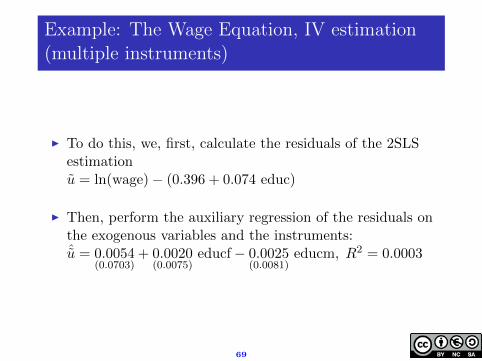
I To do this, we, first, calculate the residuals of the 2SLSestimationu = ln(wage)− (0.396 + 0.074 educ)
I Then, perform the auxiliary regression of the residuals onthe exogenous variables and the instruments:ˆu = 0.0054
(0.0703)+ 0.0020
(0.0075)educf− 0.0025
(0.0081)educm, R2 = 0.0003
69
Example: The Wage Equation, IV estimation(multiple instruments)
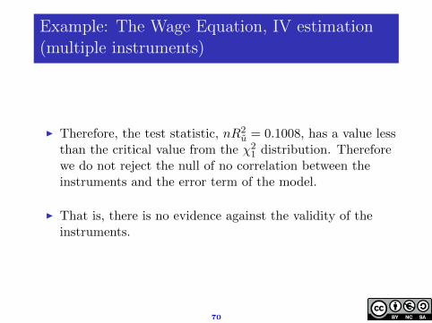
I Therefore, the test statistic, nR2u = 0.1008, has a value less
than the critical value from the χ21 distribution. Therefore
we do not reject the null of no correlation between theinstruments and the error term of the model.
I That is, there is no evidence against the validity of theinstruments.
70
Final Points
I In practice, in many situations, it is difficult to find validinstruments, that is, a variable which is not included in themodel, and is highly correlated with potentiallyendogenous explanatory variables, and is not correlatedwith the error term of the model.
I The problem is that for the economic variables, most of theavailable variables are results of agents’ decisions, andtherefore, their exogeneity is questionable.
71
Final Points
I Ideally, we would like to use, as instrumental variables,variables that are given to the agent (i.e., exogenous). Wehave seen an example the price of cigarettes as instrumentfor the number of packets of cigarettes consumed.
I The problem is that in many contexts (like the example wementioned above) the quality of the instrument is reducedby the weak correlation between the IV and theendogenous explanatory variable we use the IV for.
72
Final Points
I EXAMPLE: The availability of information about previousrealizations of the variables of interest opens interestingpossibilities for possible instruments. Thus, an endogenousexplanatory variable could be replaced by the previousrealizations of the same variable (since the previousrealizations are given before the current values are realized)
For example, for the consumption and permanent incomeequation, we use income since the forme is not available.But, we could also use the disposable income correspondingto the previous period as IV.If we analyze this relationship with aggregated time series,we could use the lagged disposable income as an instrument.If we analyze the relationship with longitudinal family data,lagged disposable income of each family could be used as aninstrument.
73