EC771: Econometrics, Spring 2011 Fractionally integrated ...fmEC771: Econometrics, Spring 2011...
27
EC771: Econometrics, Spring 2011 Fractionally integrated timeseries and ARFIMA modelling This presentation of ARFIMA modelling draws heavily from Baum and Wiggins (2000). The model of an autoregressive fractionally in- tegrated moving average process of a time- series of order (p, d, q ), denoted by ARFIMA (p, d, q ), with mean μ, may be written using operator notation as Φ(L)(1-L) d (y t - μ) = Θ(L) t , t ∼ i.i.d.(0,σ 2 ) (1) where L is the backward-shift operator, Φ(L) =1- φ 1 L - .. - φ p L p , Θ(L)=1+ ϑ 1 L + ... + ϑ q L q , and (1 - L) d is the fractional differencing operator defined by (1 - L) d = ∞ X k=0 Γ(k - d)L k Γ(-d)Γ(k + 1) (2)
Transcript of EC771: Econometrics, Spring 2011 Fractionally integrated ...fmEC771: Econometrics, Spring 2011...
EC771: Econometrics, Spring 2011
Fractionally integrated timeseries andARFIMA modelling
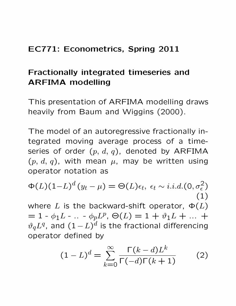
This presentation of ARFIMA modelling drawsheavily from Baum and Wiggins (2000).
The model of an autoregressive fractionally in-tegrated moving average process of a time-series of order (p, d, q), denoted by ARFIMA(p, d, q), with mean µ, may be written usingoperator notation as
Φ(L)(1−L)d (yt − µ) = Θ(L)εt, εt ∼ i.i.d.(0, σ2ε )
(1)where L is the backward-shift operator, Φ(L)= 1 - φ1L - .. - φpLp, Θ(L) = 1 + ϑ1L + ... +ϑqLq, and (1−L)d is the fractional differencingoperator defined by
(1− L)d =∞∑k=0
Γ(k − d)Lk
Γ(−d)Γ(k + 1)(2)
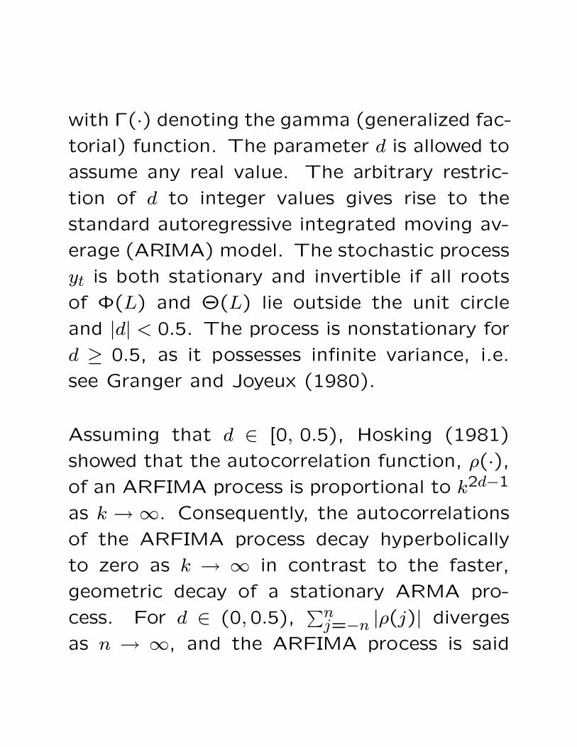
with Γ(·) denoting the gamma (generalized fac-
torial) function. The parameter d is allowed to
assume any real value. The arbitrary restric-
tion of d to integer values gives rise to the
standard autoregressive integrated moving av-
erage (ARIMA) model. The stochastic process
yt is both stationary and invertible if all roots
of Φ(L) and Θ(L) lie outside the unit circle
and |d| < 0.5. The process is nonstationary for
d ≥ 0.5, as it possesses infinite variance, i.e.
see Granger and Joyeux (1980).
Assuming that d ∈ [0, 0.5), Hosking (1981)
showed that the autocorrelation function, ρ(·),
of an ARFIMA process is proportional to k2d−1
as k → ∞. Consequently, the autocorrelations
of the ARFIMA process decay hyperbolically
to zero as k → ∞ in contrast to the faster,
geometric decay of a stationary ARMA pro-
cess. For d ∈ (0,0.5),∑nj=−n |ρ(j)| diverges
as n → ∞, and the ARFIMA process is said
to exhibit long memory, or long-range positive
dependence. The process is said to exhibit in-
termediate memory (anti-persistence), or long-
range negative dependence, for d ∈ (−0.5,0).
The process exhibits short memory for d =
0, corresponding to stationary and invertible
ARMA modeling. For d ∈ [0.5, 1) the process
is mean reverting, even though it is not covari-
ance stationary, as there is no long-run impact
of an innovation on future values of the pro-
cess.
If a series exhibits long memory, it is neither
stationary (I(0)) nor is it a unit root (I(1))
process; it is an I(d) process, with d a real
number. A series exhibiting long memory, or
persistence, has an autocorrelation function that
damps hyperbolically, more slowly than the ge-
ometric damping exhibited by “short memory”
(ARMA) processes. Thus, it may be predictable
at long horizons. An excellent survey of long
memory models–which originated in hydrology,
and have been widely applied in economics and
finance–is given in Baillie (1996). An up-to-
date survey of these models in finance is avail-
able as “Is there long memory in financial time
series?”, Lima, L. and Xiao, Z., Applied Fi-
nancial Economics, 20: 6, 487–500.
Approaches to estimation of the ARFIMA
model
There are two approaches to the estimation of
an ARFIMA (p, d, q) model: exact maximum
likelihood estimation, as proposed by Sowell
(1992), and semiparametric approaches. Sow-
ell’s approach requires specification of the p
and q values, and estimation of the full ARFIMA
model conditional on those choices. This in-
volves all the attendant difficulties of choosing
an appropriate ARMA specification, as well as
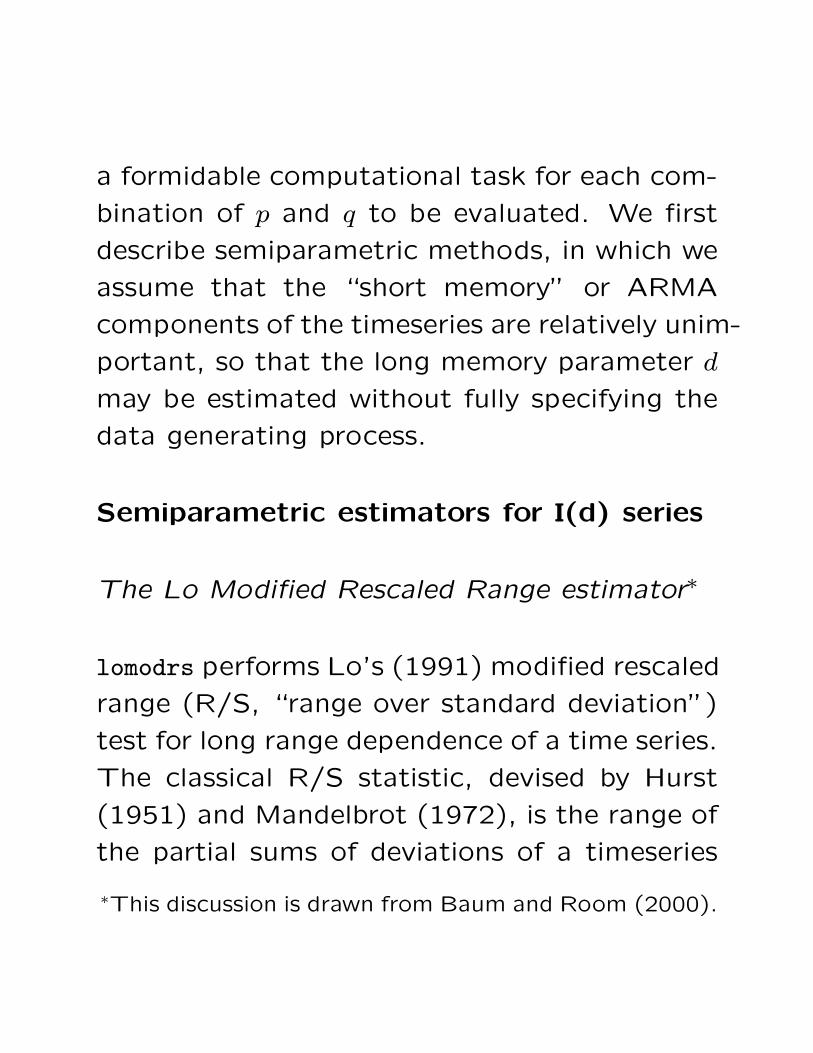
a formidable computational task for each com-
bination of p and q to be evaluated. We first
describe semiparametric methods, in which we
assume that the “short memory” or ARMA
components of the timeseries are relatively unim-
portant, so that the long memory parameter d
may be estimated without fully specifying the
data generating process.
Semiparametric estimators for I(d) series
The Lo Modified Rescaled Range estimator∗
lomodrs performs Lo’s (1991) modified rescaled
range (R/S, “range over standard deviation”)
test for long range dependence of a time series.
The classical R/S statistic, devised by Hurst
(1951) and Mandelbrot (1972), is the range of
the partial sums of deviations of a timeseries
∗This discussion is drawn from Baum and Room (2000).
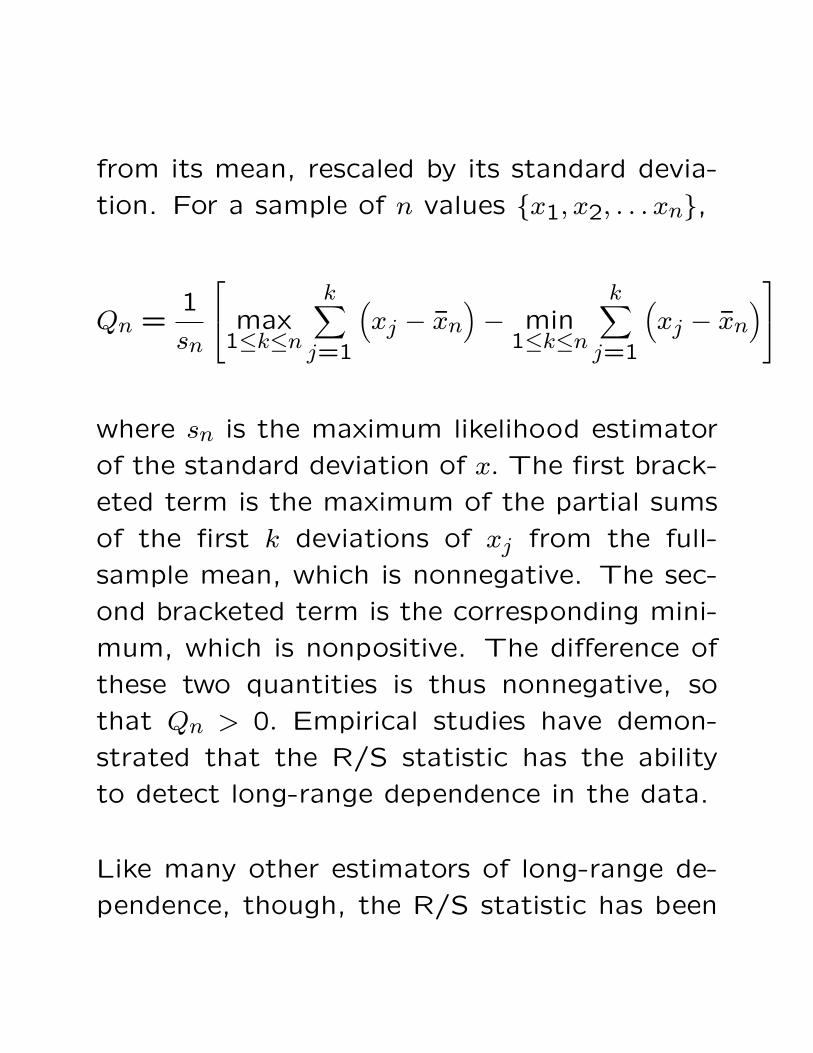
from its mean, rescaled by its standard devia-
tion. For a sample of n values {x1, x2, . . . xn},
Qn =1
sn
max1≤k≤n
k∑j=1
(xj − xn
)− min
1≤k≤n
k∑j=1
(xj − xn
)
where sn is the maximum likelihood estimator
of the standard deviation of x. The first brack-
eted term is the maximum of the partial sums
of the first k deviations of xj from the full-
sample mean, which is nonnegative. The sec-
ond bracketed term is the corresponding mini-
mum, which is nonpositive. The difference of
these two quantities is thus nonnegative, so
that Qn > 0. Empirical studies have demon-
strated that the R/S statistic has the ability
to detect long-range dependence in the data.
Like many other estimators of long-range de-
pendence, though, the R/S statistic has been
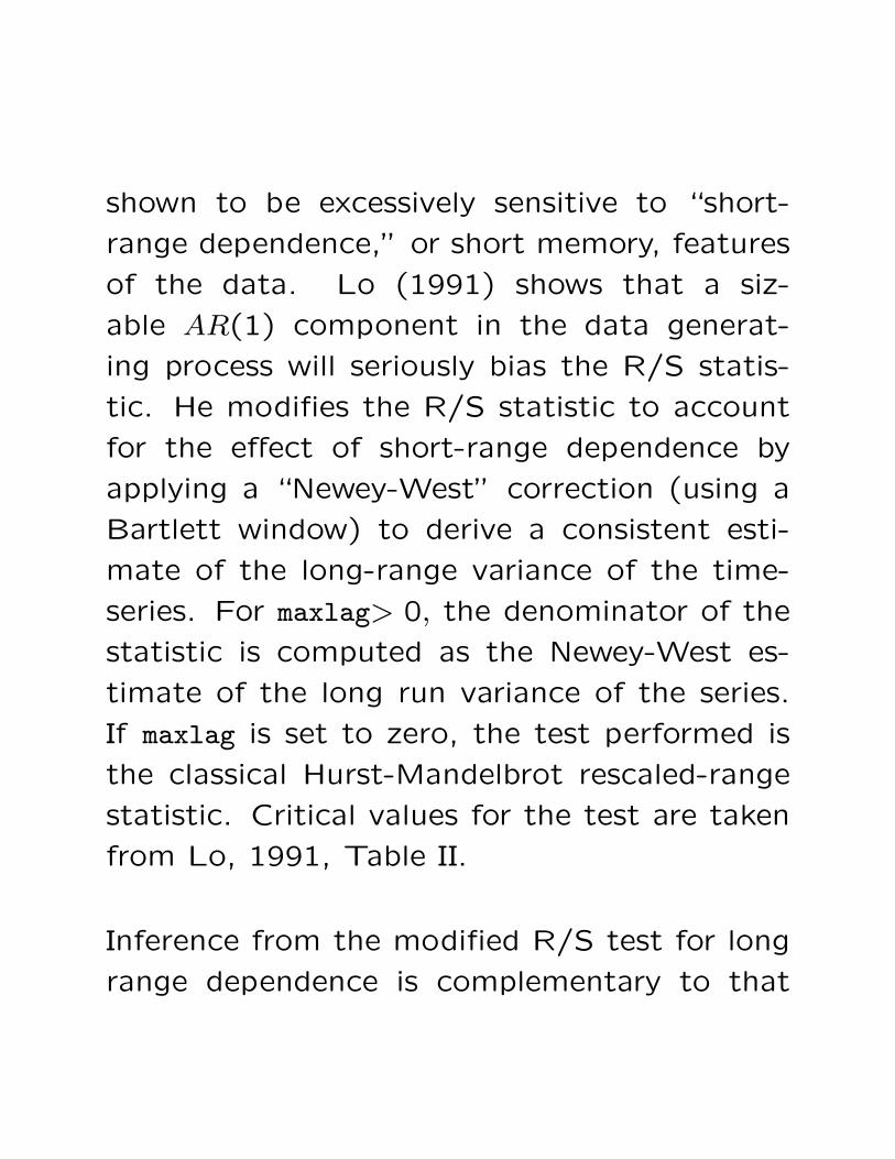
shown to be excessively sensitive to “short-
range dependence,” or short memory, features
of the data. Lo (1991) shows that a siz-
able AR(1) component in the data generat-
ing process will seriously bias the R/S statis-
tic. He modifies the R/S statistic to account
for the effect of short-range dependence by
applying a “Newey-West” correction (using a
Bartlett window) to derive a consistent esti-
mate of the long-range variance of the time-
series. For maxlag> 0, the denominator of the
statistic is computed as the Newey-West es-
timate of the long run variance of the series.
If maxlag is set to zero, the test performed is
the classical Hurst-Mandelbrot rescaled-range
statistic. Critical values for the test are taken
from Lo, 1991, Table II.
Inference from the modified R/S test for long
range dependence is complementary to that
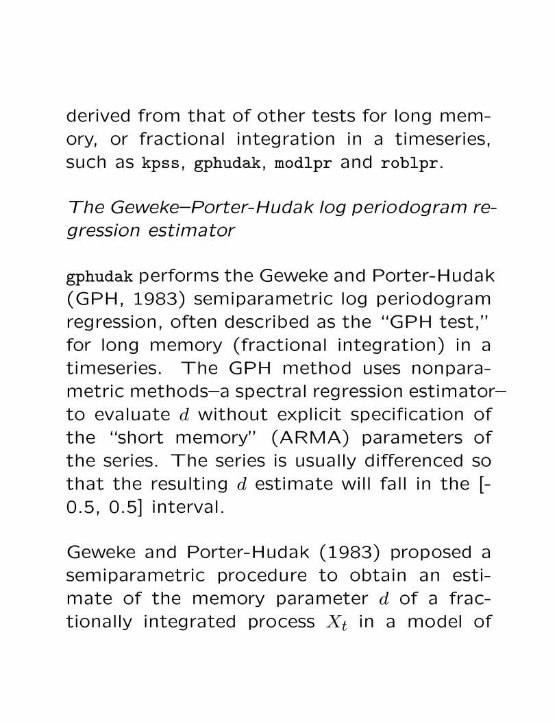
derived from that of other tests for long mem-ory, or fractional integration in a timeseries,such as kpss, gphudak, modlpr and roblpr.
The Geweke–Porter-Hudak log periodogram re-gression estimator
gphudak performs the Geweke and Porter-Hudak(GPH, 1983) semiparametric log periodogramregression, often described as the “GPH test,”for long memory (fractional integration) in atimeseries. The GPH method uses nonpara-metric methods–a spectral regression estimator–to evaluate d without explicit specification ofthe “short memory” (ARMA) parameters ofthe series. The series is usually differenced sothat the resulting d estimate will fall in the [-0.5, 0.5] interval.
Geweke and Porter-Hudak (1983) proposed asemiparametric procedure to obtain an esti-mate of the memory parameter d of a frac-tionally integrated process Xt in a model of
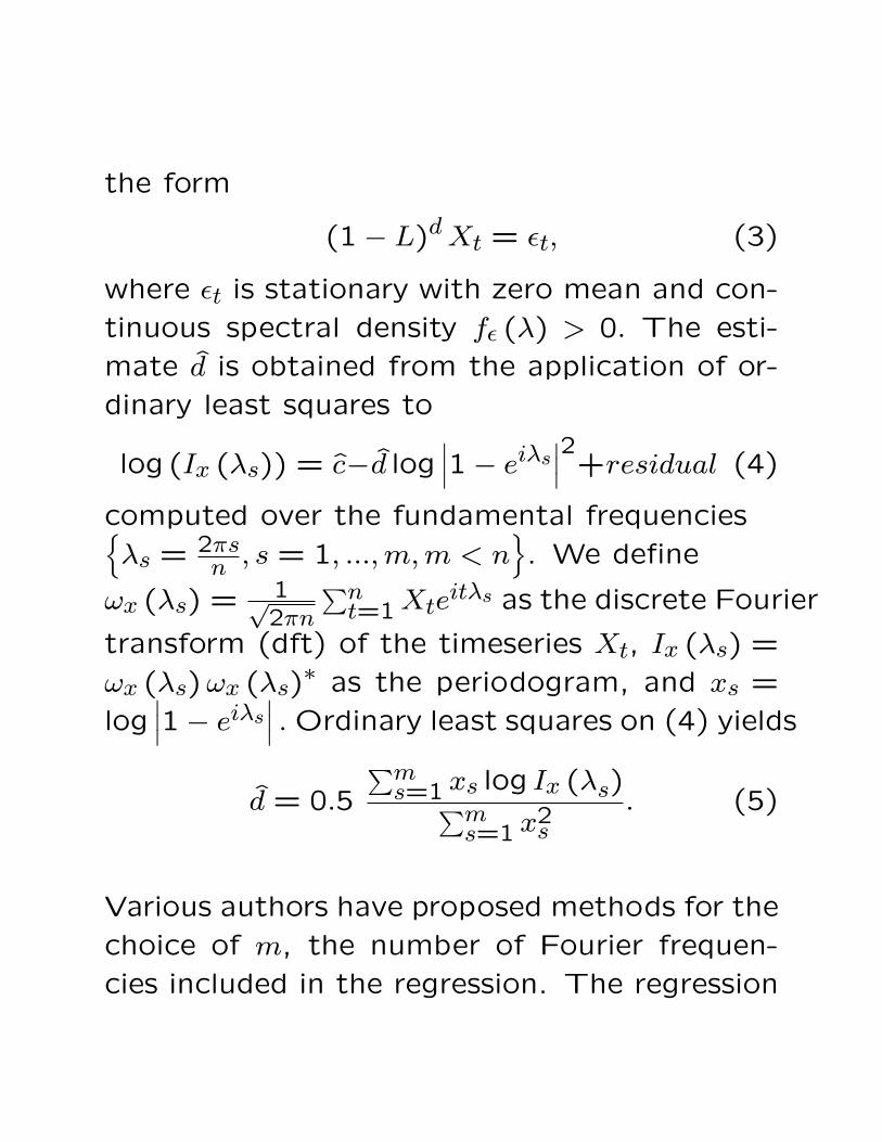
the form
(1− L)dXt = εt, (3)
where εt is stationary with zero mean and con-
tinuous spectral density fε (λ) > 0. The esti-
mate d is obtained from the application of or-
dinary least squares to
log (Ix (λs)) = c−d log∣∣∣1− eiλs∣∣∣2+residual (4)
computed over the fundamental frequencies{λs = 2πs
n , s = 1, ...,m,m < n}
. We define
ωx (λs) = 1√2πn
∑nt=1Xte
itλs as the discrete Fourier
transform (dft) of the timeseries Xt, Ix (λs) =
ωx (λs)ωx (λs)∗ as the periodogram, and xs =
log∣∣∣1− eiλs∣∣∣ . Ordinary least squares on (4) yields
d = 0.5
∑ms=1 xs log Ix (λs)∑m
s=1 x2s
. (5)
Various authors have proposed methods for the
choice of m, the number of Fourier frequen-
cies included in the regression. The regression
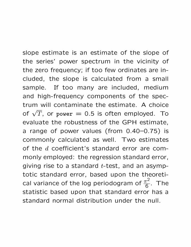
slope estimate is an estimate of the slope of
the series’ power spectrum in the vicinity of
the zero frequency; if too few ordinates are in-
cluded, the slope is calculated from a small
sample. If too many are included, medium
and high-frequency components of the spec-
trum will contaminate the estimate. A choice
of√T , or power = 0.5 is often employed. To
evaluate the robustness of the GPH estimate,
a range of power values (from 0.40–0.75) is
commonly calculated as well. Two estimates
of the d coefficient’s standard error are com-
monly employed: the regression standard error,
giving rise to a standard t-test, and an asymp-
totic standard error, based upon the theoreti-
cal variance of the log periodogram of π2
6 . The
statistic based upon that standard error has a
standard normal distribution under the null.
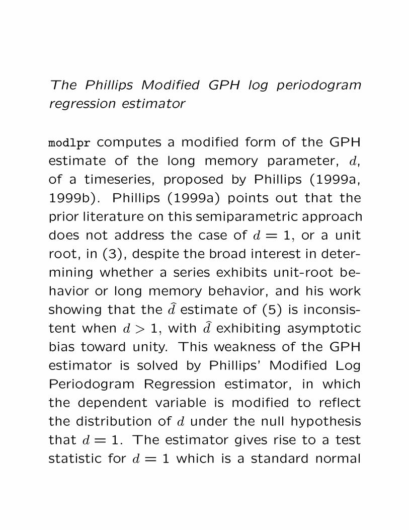
The Phillips Modified GPH log periodogram
regression estimator
modlpr computes a modified form of the GPH
estimate of the long memory parameter, d,
of a timeseries, proposed by Phillips (1999a,
1999b). Phillips (1999a) points out that the
prior literature on this semiparametric approach
does not address the case of d = 1, or a unit
root, in (3), despite the broad interest in deter-
mining whether a series exhibits unit-root be-
havior or long memory behavior, and his work
showing that the d estimate of (5) is inconsis-
tent when d > 1, with d exhibiting asymptotic
bias toward unity. This weakness of the GPH
estimator is solved by Phillips’ Modified Log
Periodogram Regression estimator, in which
the dependent variable is modified to reflect
the distribution of d under the null hypothesis
that d = 1. The estimator gives rise to a test
statistic for d = 1 which is a standard normal

variate under the null. Phillips suggests that
deterministic trends should be removed from
the series before application of the estimator.
Accordingly, the routine will automatically re-
move a linear trend from the series. This may
be suppressed with the notrend option. The
comments above regarding power apply equally
to modlpr.
Phillips’ (1999b) modification of the GPH es-
timator is based on an exact representation of
the dft in the unit root case. The modification
expresses
ωx (λs) =ωu (λs)
1− eiλs−
eiλs
1− eiλsXn√2πn
and the modified dft as
υx (λs) = ωx (λs) +eiλs
1− eiλsXn√2πn
with associated periodogram ordinates
Iv (λs) = υx (λs) υx (λs)∗ (1999b, p.9). He notes
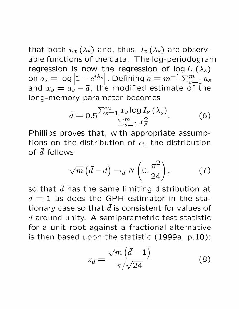
that both υx (λs) and, thus, Iv (λs) are observ-able functions of the data. The log-periodogramregression is now the regression of log Iv (λs)on as = log
∣∣∣1− eiλs∣∣∣ . Defining a = m−1∑ms=1 as
and xs = as − a, the modified estimate of thelong-memory parameter becomes
d = 0.5
∑ms=1 xs log Iν (λs)∑m
s=1 x2s
. (6)
Phillips proves that, with appropriate assump-tions on the distribution of εt, the distributionof d follows
√m(d− d
)→d N
(0,π2
24
), (7)
so that d has the same limiting distribution atd = 1 as does the GPH estimator in the sta-tionary case so that d is consistent for values ofd around unity. A semiparametric test statisticfor a unit root against a fractional alternativeis then based upon the statistic (1999a, p.10):
zd =
√m(d− 1
)π/√
24(8)
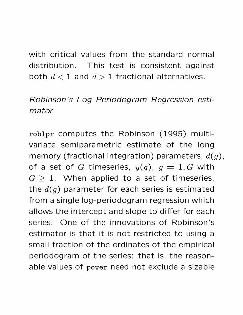
with critical values from the standard normal
distribution. This test is consistent against
both d < 1 and d > 1 fractional alternatives.
Robinson’s Log Periodogram Regression esti-
mator
roblpr computes the Robinson (1995) multi-
variate semiparametric estimate of the long
memory (fractional integration) parameters, d(g),
of a set of G timeseries, y(g), g = 1, G with
G ≥ 1. When applied to a set of timeseries,
the d(g) parameter for each series is estimated
from a single log-periodogram regression which
allows the intercept and slope to differ for each
series. One of the innovations of Robinson’s
estimator is that it is not restricted to using a
small fraction of the ordinates of the empirical
periodogram of the series: that is, the reason-
able values of power need not exclude a sizable
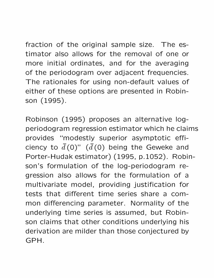
fraction of the original sample size. The es-
timator also allows for the removal of one or
more initial ordinates, and for the averaging
of the periodogram over adjacent frequencies.
The rationales for using non-default values of
either of these options are presented in Robin-
son (1995).
Robinson (1995) proposes an alternative log-
periodogram regression estimator which he claims
provides “modestly superior asymptotic effi-
ciency to d (0)” (d (0) being the Geweke and
Porter-Hudak estimator) (1995, p.1052). Robin-
son’s formulation of the log-periodogram re-
gression also allows for the formulation of a
multivariate model, providing justification for
tests that different time series share a com-
mon differencing parameter. Normality of the
underlying time series is assumed, but Robin-
son claims that other conditions underlying his
derivation are milder than those conjectured by
GPH.
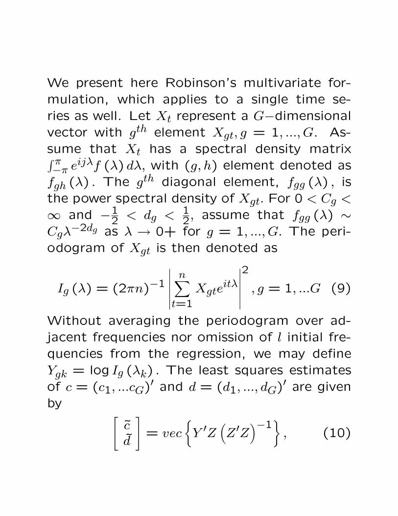
We present here Robinson’s multivariate for-mulation, which applies to a single time se-ries as well. Let Xt represent a G−dimensionalvector with gth element Xgt, g = 1, ..., G. As-sume that Xt has a spectral density matrix∫ π−π e
ijλf (λ) dλ, with (g, h) element denoted asfgh (λ) . The gth diagonal element, fgg (λ) , isthe power spectral density of Xgt. For 0 < Cg <
∞ and −12 < dg < 1
2, assume that fgg (λ) ∼Cgλ−2dg as λ → 0+ for g = 1, ..., G. The peri-odogram of Xgt is then denoted as
Ig (λ) = (2πn)−1
∣∣∣∣∣∣n∑t=1
Xgteitλ
∣∣∣∣∣∣2
, g = 1, ...G (9)
Without averaging the periodogram over ad-jacent frequencies nor omission of l initial fre-quencies from the regression, we may defineYgk = log Ig (λk) . The least squares estimatesof c = (c1, ...cG)′ and d = (d1, ..., dG)′ are givenby [
cd
]= vec
{Y ′Z
(Z′Z
)−1}, (10)
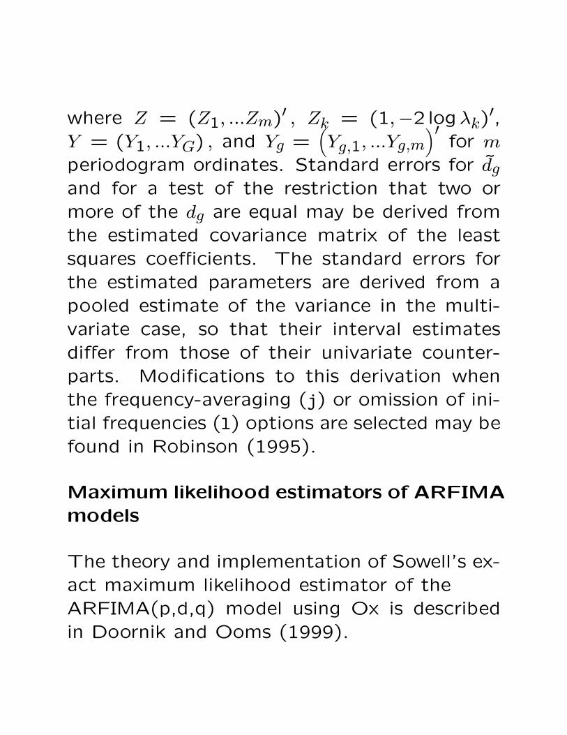
where Z = (Z1, ...Zm)′ , Zk = (1,−2 logλk)′,Y = (Y1, ...YG) , and Yg =
(Yg,1, ...Yg,m
)′for m
periodogram ordinates. Standard errors for dgand for a test of the restriction that two ormore of the dg are equal may be derived fromthe estimated covariance matrix of the leastsquares coefficients. The standard errors forthe estimated parameters are derived from apooled estimate of the variance in the multi-variate case, so that their interval estimatesdiffer from those of their univariate counter-parts. Modifications to this derivation whenthe frequency-averaging (j) or omission of ini-tial frequencies (l) options are selected may befound in Robinson (1995).
Maximum likelihood estimators of ARFIMAmodels
The theory and implementation of Sowell’s ex-act maximum likelihood estimator of theARFIMA(p,d,q) model using Ox is describedin Doornik and Ooms (1999).
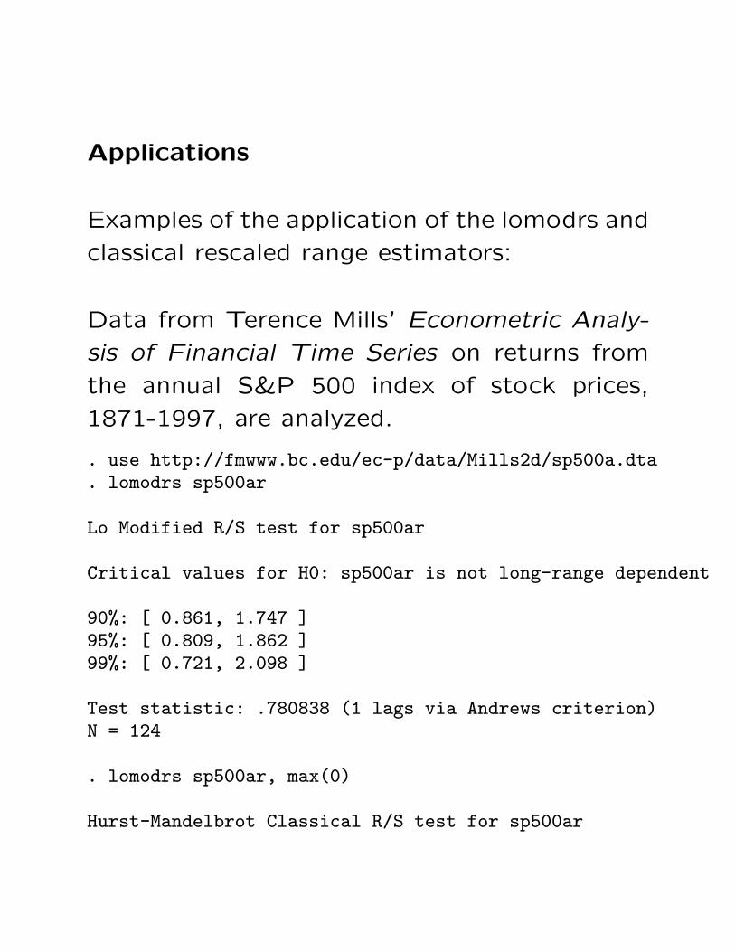
Applications
Examples of the application of the lomodrs and
classical rescaled range estimators:
Data from Terence Mills’ Econometric Analy-
sis of Financial Time Series on returns from
the annual S&P 500 index of stock prices,
1871-1997, are analyzed.
. use http://fmwww.bc.edu/ec-p/data/Mills2d/sp500a.dta
. lomodrs sp500ar
Lo Modified R/S test for sp500ar
Critical values for H0: sp500ar is not long-range dependent
90%: [ 0.861, 1.747 ]95%: [ 0.809, 1.862 ]99%: [ 0.721, 2.098 ]
Test statistic: .780838 (1 lags via Andrews criterion)N = 124
. lomodrs sp500ar, max(0)
Hurst-Mandelbrot Classical R/S test for sp500ar
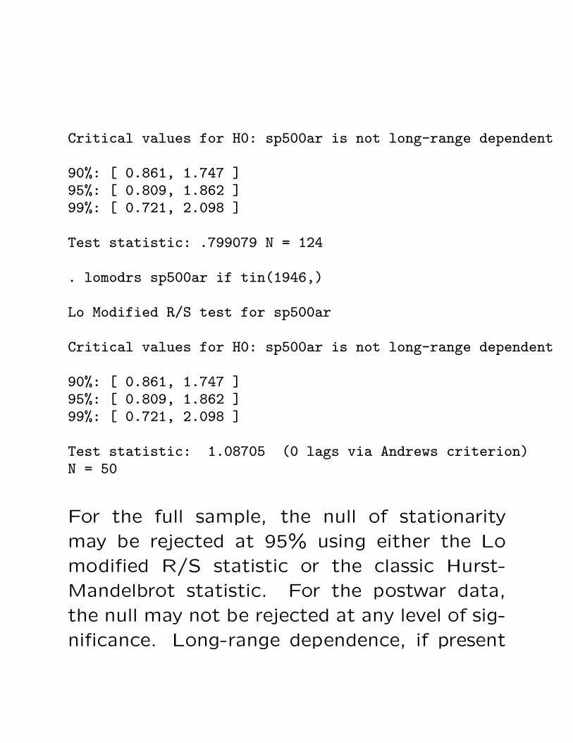
Critical values for H0: sp500ar is not long-range dependent
90%: [ 0.861, 1.747 ]95%: [ 0.809, 1.862 ]99%: [ 0.721, 2.098 ]
Test statistic: .799079 N = 124
. lomodrs sp500ar if tin(1946,)
Lo Modified R/S test for sp500ar
Critical values for H0: sp500ar is not long-range dependent
90%: [ 0.861, 1.747 ]95%: [ 0.809, 1.862 ]99%: [ 0.721, 2.098 ]
Test statistic: 1.08705 (0 lags via Andrews criterion)N = 50
For the full sample, the null of stationaritymay be rejected at 95% using either the Lomodified R/S statistic or the classic Hurst-Mandelbrot statistic. For the postwar data,the null may not be rejected at any level of sig-nificance. Long-range dependence, if present

in this series, seems to be contributed by pre-
World War II behavior of the stock price series.
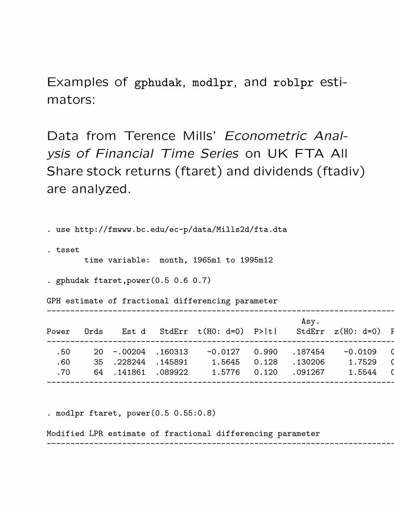
Examples of gphudak, modlpr, and roblpr esti-
mators:
Data from Terence Mills’ Econometric Anal-
ysis of Financial Time Series on UK FTA All
Share stock returns (ftaret) and dividends (ftadiv)
are analyzed.
. use http://fmwww.bc.edu/ec-p/data/Mills2d/fta.dta
. tssettime variable: month, 1965m1 to 1995m12
. gphudak ftaret,power(0.5 0.6 0.7)
GPH estimate of fractional differencing parameter------------------------------------------------------------------------------
Asy.Power Ords Est d StdErr t(H0: d=0) P>|t| StdErr z(H0: d=0) P>|z|------------------------------------------------------------------------------
.50 20 -.00204 .160313 -0.0127 0.990 .187454 -0.0109 0.991
.60 35 .228244 .145891 1.5645 0.128 .130206 1.7529 0.080
.70 64 .141861 .089922 1.5776 0.120 .091267 1.5544 0.120------------------------------------------------------------------------------
. modlpr ftaret, power(0.5 0.55:0.8)
Modified LPR estimate of fractional differencing parameter------------------------------------------------------------------------------
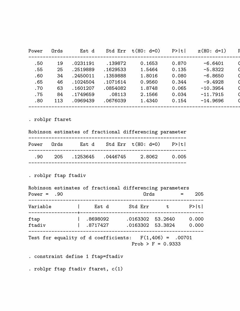
Power Ords Est d Std Err t(H0: d=0) P>|t| z(H0: d=1) P>|z|------------------------------------------------------------------------------
.50 19 .0231191 .139872 0.1653 0.870 -6.6401 0.000
.55 25 .2519889 .1629533 1.5464 0.135 -5.8322 0.000
.60 34 .2450011 .1359888 1.8016 0.080 -6.8650 0.000
.65 46 .1024504 .1071614 0.9560 0.344 -9.4928 0.000
.70 63 .1601207 .0854082 1.8748 0.065 -10.3954 0.000
.75 84 .1749659 .08113 2.1566 0.034 -11.7915 0.000
.80 113 .0969439 .0676039 1.4340 0.154 -14.9696 0.000------------------------------------------------------------------------------
. roblpr ftaret
Robinson estimates of fractional differencing parameter-------------------------------------------------------Power Ords Est d Std Err t(H0: d=0) P>|t|-------------------------------------------------------
.90 205 .1253645 .0446745 2.8062 0.005-------------------------------------------------------
. roblpr ftap ftadiv
Robinson estimates of fractional differencing parametersPower = .90 Ords = 205-------------------------------------------------------------Variable | Est d Std Err t P>|t|-----------------+-------------------------------------------ftap | .8698092 .0163302 53.2640 0.000ftadiv | .8717427 .0163302 53.3824 0.000-------------------------------------------------------------Test for equality of d coefficients: F(1,406) = .00701
Prob > F = 0.9333
. constraint define 1 ftap=ftadiv
. roblpr ftap ftadiv ftaret, c(1)
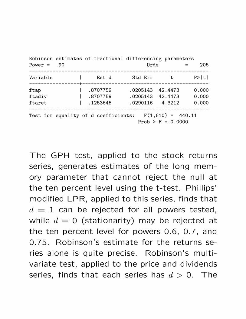
Robinson estimates of fractional differencing parametersPower = .90 Ords = 205-------------------------------------------------------------Variable | Est d Std Err t P>|t|-----------------+-------------------------------------------ftap | .8707759 .0205143 42.4473 0.000ftadiv | .8707759 .0205143 42.4473 0.000ftaret | .1253645 .0290116 4.3212 0.000-------------------------------------------------------------Test for equality of d coefficients: F(1,610) = 440.11
Prob > F = 0.0000
The GPH test, applied to the stock returns
series, generates estimates of the long mem-
ory parameter that cannot reject the null at
the ten percent level using the t-test. Phillips’
modified LPR, applied to this series, finds that
d = 1 can be rejected for all powers tested,
while d = 0 (stationarity) may be rejected at
the ten percent level for powers 0.6, 0.7, and
0.75. Robinson’s estimate for the returns se-
ries alone is quite precise. Robinson’s multi-
variate test, applied to the price and dividends
series, finds that each series has d > 0. The
test that they share the same d cannot be re-jected. Accordingly, the test is applied to allthree series subject to the constraint that priceand dividends series have a common d, yieldinga more precise estimate of the difference in d
parameters between those series and the stockreturns series.
References
Andrews, D., 1991. Heteroskedasticity andAutocorrelation Consistent Covariance MatrixEstimation. Econometrica, 59, 817-858.
Baillie, R. 1996. Long Memory Processes andFractional Integration in Econometrics, Jour-nal of Econometrics, 73, 5-59.
Baum, Christopher F and Tairi Room, 2000.The modified rescaled range test for long mem-ory. Help file for Stata module lomodrs, avail-able from SSC-IDEAS at http://ideas.repec.org.
Baum, Christopher F and Vince Wiggins, 2000.
Tests for long memory in a timeseries. Stata
Technical Bulletin 57, available from SSC-IDEAS
at http://ideas.repec.org.
Doornik, Jurgen A. and Marius Ooms. 1999.
A package for estimating, forecasting and sim-
ulating Arfima Models: Arfima package 1.0 for
Ox.
Geweke, J. and Porter-Hudak, S. 1983. The
Estimation and Application of Long Memory
Time Series Models, Journal of Time Series
Analysis, 221-238.
Granger, C. W. J. and R. Joyeux. 1980. An
introduction to long-memory time series mod-
els and fractional differencing, Journal of Time
Series Analysis, 1, 15-39.
Hosking, J. R. M. 1981. Fractional Differenc-
ing, Biometrika, 68, 165-176.
Hurst, H., 1951. Long Term Storage Capacity
of Reservoirs. Transactions of the American
Society of Civil Engineers, 116, 770-799.
Lima, L. and Xiao, Z., 2010. Is there long
memory in financial time series?, Applied Fi-
nancial Economics, 20:6, 487–500.
Lo, Andrew W., 1991. Long-Term Memory in
Stock Market Prices. Econometrica, 59, 1991,
1279-1313.
Mandelbrot, B., 1972. Statistical Methodol-
ogy for Non-Periodic Cycles: From the Co-
variance to R/S Analysis. Annals of Economic
and Social Measurement, 1, 259-290.
Phillips, Peter C.B. 1999a. Discrete Fourier
Transforms of Fractional Processes, Unpub-
lished working paper No. 1243, Cowles Foun-
dation for Research in Economics, Yale Uni-
versity.
Phillips, Peter C.B. 1999b. Unit Root Log
Periodogram Regression, Unpublished working
paper No. 1244, Cowles Foundation for Re-
search in Economics, Yale University.
Robinson, P.M. 1995. Log-Periodogram Re-
gression of Time Series with Long Range De-
pendence. Annals of Statistics, 23:3, 1048-
1072.
Sowell, F. 1992. Maximum likelihood estima-
tion of stationary univariate fractionally-integrated
time-series models, Journal of Econometrics,
53, 165-188.