E2LSH 0.1User Manual

Alexandr AndoniPiotr Indyk

June 21, 2005

Contents

1 What is E2LSH? 2

2 E2LSH Usage 42.1 Compilation . . . . . . . . . . . . . . . . . . . . . . . . . . . . . . . . . . . . .. . . . . . 42.2 Main Usage . . . . . . . . . . . . . . . . . . . . . . . . . . . . . . . . . . . . . . .. . . . 42.3 Manual setting of the parameters of theR-NN data structure . . . . . . . . . . . . . . . . . 42.4 Memory . . . . . . . . . . . . . . . . . . . . . . . . . . . . . . . . . . . . . . . . . .. . . 62.5 Additional utilities . . . . . . . . . . . . . . . . . . . . . . . . . . . . .. . . . . . . . . . 62.6 File formats . . . . . . . . . . . . . . . . . . . . . . . . . . . . . . . . . . . . .. . . . . . 6

2.6.1 Data set file and query set file . . . . . . . . . . . . . . . . . . . . . .. . . . . . . 62.6.2 Output file format . . . . . . . . . . . . . . . . . . . . . . . . . . . . . . .. . . . . 72.6.3 File with the parameters for theR-NN data structure . . . . . . . . . . . . . . . . . 72.6.4 The remainder of the parameter file . . . . . . . . . . . . . . . . .. . . . . . . . . 8

3 Algorithm description 93.1 Notations . . . . . . . . . . . . . . . . . . . . . . . . . . . . . . . . . . . . . . .. . . . . 93.2 Generic locality-sensitive hashing scheme . . . . . . . . . .. . . . . . . . . . . . . . . . . 93.3 LSH scheme forlp norm . . . . . . . . . . . . . . . . . . . . . . . . . . . . . . . . . . . . 10

3.3.1 p-stable distributions . . . . . . . . . . . . . . . . . . . . . . . . . . . . . . .. . . 103.3.2 Hash family . . . . . . . . . . . . . . . . . . . . . . . . . . . . . . . . . . . .. . . 10

3.4 Parameters for the LSH scheme . . . . . . . . . . . . . . . . . . . . . . .. . . . . . . . . 113.4.1 Faster computation of hash functions . . . . . . . . . . . . . .. . . . . . . . . . . 12

3.5 Implementation details . . . . . . . . . . . . . . . . . . . . . . . . . . .. . . . . . . . . . 123.5.1 R-NN data structure construction . . . . . . . . . . . . . . . . . . . . . . .. . . . 123.5.2 Bucket hashing . . . . . . . . . . . . . . . . . . . . . . . . . . . . . . . . .. . . . 133.5.3 Additional optimizations . . . . . . . . . . . . . . . . . . . . . . .. . . . . . . . . 14

3.6 Memory . . . . . . . . . . . . . . . . . . . . . . . . . . . . . . . . . . . . . . . . . .. . . 143.7 Future possible optimizations . . . . . . . . . . . . . . . . . . . . .. . . . . . . . . . . . . 15

4 The E2LSH Code 164.1 Code overview . . . . . . . . . . . . . . . . . . . . . . . . . . . . . . . . . . . .. . . . . 164.2 E2LSH Interface . . . . . . . . . . . . . . . . . . . . . . . . . . . . . . . . . . . . . . .. 17

5 Frequent Anticipated Questions 20

1

Chapter 1

What is E2LSH?

Short answer:E2LSH (Exact Euclidean LSH) is a package that provides a randomized solution for the high-dimensional

near neighbor problem in the Euclidean spacel2. After preprocessing the data set, E2LSH answers queries,typically in sublinear time, with each near neighbor being reported with a certain probability. E2LSH isbased on the Locality Sensitive Hashing (LSH) scheme described in [2].

Long answer:TheR-near neighbor problem is defined as follows. Given a set of pointsP ⊂ Rd and a radiusR > 0,

construct a data structure that answers the following queries: for a query pointq, find all pointsp ∈ Psuch that||q − p||2 ≤ R, where||q − p||2 is the Euclidean distance betweenq andp. E2LSH solves arandomized version of this problem, which we call a(R, 1 − δ)-near neighbor problem. In this case, eachpointp satisfying||q−p||2 ≤ R has to be reported with a probability at least1− δ (thus,δ is the probabilitythat a near neighborp is not reported).

E2LSH can be also used to solve thenearest neighbor problem, where, given the queryq, the datastructure is required the report the point inP that is closest toq. This can be done by creating severalR-nearneighbor data structures, forR = R1, R2, . . . Rt, whereRt should be greater than the maximum distancefrom any query point to its nearest neighbor. The nearest neighbor can be then recovered by querying thedata structures in the increasing order of the radiae, stopping whenever the first point is found.

E2LSH is based on locality-sensitive hashing (LSH) scheme, asdescribed in [2]. The original locality-sensitive hashing scheme solves theapproximate version of theR-near neighbor problem, called a(R, c)-near neighbor problem. In that formulation, it is sufficientto reportany point within the distance of at mostcR from the queryq, if there is a point inP at distance at mostR from q (with a constant probability). Forthe approximate formulation, the LSH scheme achieves a timeof O(nρ), whereρ < 1/c.

To solve the(R, 1 − δ) formulation, E2LSH uses the basic LSH scheme to get all near neighbors (in-cluding the approximate ones), and then drops the approximate near neighbors. Thus, the running time ofE2LSH depends on the data setP. In particular, E2LSH is slower for “bad” data sets, e.g., when for a queryq, there are many points fromP clustered right outside the ball of radiusR centered atq (i.e., when thereare many approximate near neighbors).

E2LSH is also different from the original LSH scheme in that E2LSH empirically estimates the optimalparameters for the data structure, as opposed to using theoretical formulas. This is because theoreticalformulas are geared towards the worst case point sets, and therefore they are less adequate for the real data

2

sets. E2LSH computes the parameters as a function of the data setP and optimizes them to minimize theactual running time of query on the host system.

The outline of the remaining part of the manual is as follows.Chapter 2 describes the package and howto use it to solve the near neighbor problem. In Chapter 3, we describe the LSH algorithm used to solve the(R, 1 − δ) problem formulation, as well as optimizations for decreasing running time and memory usage.Chapter 4 discusses the structure of the code of the E2LSH: the main data types and modules, as well as themain functions for constructing, parametrizing and querying the data structure. Finally, Chapter 5 containsFAQ.

3

Chapter 2

E2LSH Usage

In this chapter, we describe how to use our E2LSH package. First, we show how to compile and use themain script of the package; and then we describe two additional scripts to use when one wants to modify orset manually the parameters of theR-NN data structure. Next, we elaborate on memory usage of E2LSHand how to control it. Finally, we present some additional useful utilities, as well as the formats of the datafiles of the package.

All the scripts and programs should be located in thebin directory relative to the E2LSH package rootdirectory.

2.1 Compilation

To compile the E2LSH package, it is sufficient to runmake from E2LSH’s root directory. It is also possibleto compile by running the scriptbin/compile from E2LSH’s root directory.

2.2 Main Usage

The main script of E2LSH is bin/lsh . It is invoked as follows:

bin/lsh R data_set_file query_set_file [successProbabil ity]

The script takes, as its parameters, the namedata set file of the file with the data set points and thefile query set file with the query points (the format of the files is described in Section 2.6). Given thesefiles, E2LSH constructs the optimizedR-NN data structure, and then runs the queries on the constructed datastructure. The valuesRandsuccessProbability specify the parametersR and1−δ of the(R, 1−δ)-near neighbor problem that E2LSH solves. Note thatsuccessProbability is an optional parameter; ifnot supplied, E2LSH uses a default value of0.9 (90% success probability).

2.3 Manual setting of the parameters of theR-NN data structure

As described in Chapter 3, the LSH data structure needs threeparameters, denoted byk, L andm (wherem ≈

√L). However, the scriptbin/lsh computes those parameters automatically in the first stage of data

structure construction. The parameters are chosen so that to optimize the estimated query time. However,

4

since these parameters are only estimates, there are no guarantees that these parameters are optimal forparticular query points. Therefore, manual setting of these parameters may occasionally provide betterquery times.

There are two additional scripts that give the possibility of manual setting of the parameters:bin/lsh computeParams andbin/lsh fromParams . The first script,bin/lsh computeParams ,computes the optimal parameters for theR-NN data structure from the given data set points and outputstheparameters to the standard output. The usage ofbin/lsh computeParams is as follows:

bin/lsh_computeParams R data_set_file {query_set_file | .} [successProbability]

The script outputs an estimation of the optimal parameters of the R-NN data structure for the data setpoints indata set file . If one specifies the query set file as the third parameter, then we use several ofthe points from the query set for optimizing data structure parameters; if a dot (. ) is specified, then we useinstead several points from the data set for the same purpose. The output is written to standard output andmay be redirected to a file (for a later use) as follows:

bin/lsh_computeParams R data_set_file query_set_file > d ata_set_parameters_file

See section 2.6 for description of the format of the parameter file.The second script,bin/lsh fromParams , takes as an input a file containing the parameters for the

R-NN data structure (besides the files with the data set pointsand the query points). The script constructsthe data structure given these parameters and runs queries on the constructed data structure. The usage ofbin/lsh fromParams is the following:

bin/lsh_fromParams data_set_file query_set_file data_s et_params_file

The filedata set params file must be of the same format as the output ofbin/lsh computeParams . Note that one does not need to specify the success probability andR sincethese values are embedded in the filedata set params file .

Thus, running the following two lines

bin/lsh_computeParams R data_set_file query_set_file > d ata_set_parameters_filebin/lsh_fromParams data_set_file query_set_file data_s et_params_file

is equivalent to running

bin/lsh R data_set_file query_set_file

To modify manually the parameters for theR-NN data structure, one should modify the filedata set params file before running the scriptbin/lsh fromParams .

For ease of use, the scriptbin/lsh also outputs the parameters it used for the constructedR-near neigh-bor data structure. These parameters are written to the filedata set file.params , wheredata set fileis the name of the supplied data set file.

5

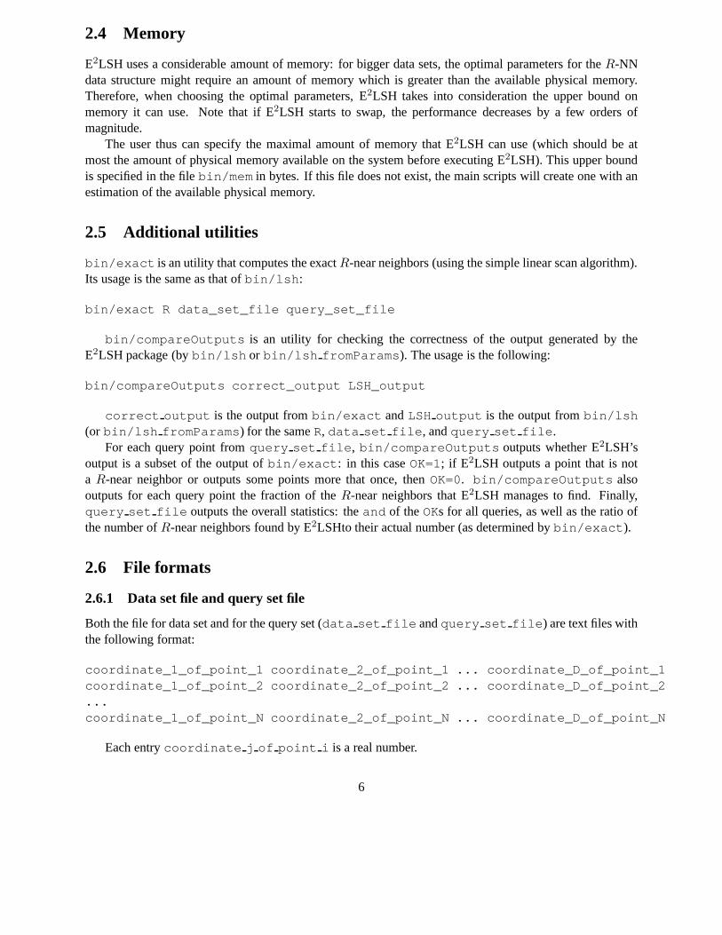
2.4 Memory

E2LSH uses a considerable amount of memory: for bigger data sets, the optimal parameters for theR-NNdata structure might require an amount of memory which is greater than the available physical memory.Therefore, when choosing the optimal parameters, E2LSH takes into consideration the upper bound onmemory it can use. Note that if E2LSH starts to swap, the performance decreases by a few ordersofmagnitude.

The user thus can specify the maximal amount of memory that E2LSH can use (which should be atmost the amount of physical memory available on the system before executing E2LSH). This upper boundis specified in the filebin/mem in bytes. If this file does not exist, the main scripts will create one with anestimation of the available physical memory.

2.5 Additional utilities

bin/exact is an utility that computes the exactR-near neighbors (using the simple linear scan algorithm).Its usage is the same as that ofbin/lsh :

bin/exact R data_set_file query_set_file

bin/compareOutputs is an utility for checking the correctness of the output generated by theE2LSH package (bybin/lsh or bin/lsh fromParams ). The usage is the following:

bin/compareOutputs correct_output LSH_output

correct output is the output frombin/exact andLSH output is the output frombin/lsh(or bin/lsh fromParams ) for the sameR, data set file , andquery set file .

For each query point fromquery set file , bin/compareOutputs outputs whether E2LSH’soutput is a subset of the output ofbin/exact : in this caseOK=1; if E2LSH outputs a point that is nota R-near neighbor or outputs some points more that once, thenOK=0. bin/compareOutputs alsooutputs for each query point the fraction of theR-near neighbors that E2LSH manages to find. Finally,query set file outputs the overall statistics: theand of theOKs for all queries, as well as the ratio ofthe number ofR-near neighbors found by E2LSHto their actual number (as determined bybin/exact ).

2.6 File formats

2.6.1 Data set file and query set file

Both the file for data set and for the query set (data set file andquery set file ) are text files withthe following format:

coordinate_1_of_point_1 coordinate_2_of_point_1 ... co ordinate_D_of_point_1coordinate_1_of_point_2 coordinate_2_of_point_2 ... co ordinate_D_of_point_2...coordinate_1_of_point_N coordinate_2_of_point_N ... co ordinate_D_of_point_N

Each entrycoordinate j of point i is a real number.

6

2.6.2 Output file format

The output of E2LSH is twofold. The main results are directed to standard output (cout ). The outputstream has the following format:

Query point i : found x NNs. They are:............Total time for R-NN query: y

Additional information is reported to standard error (cerr ).

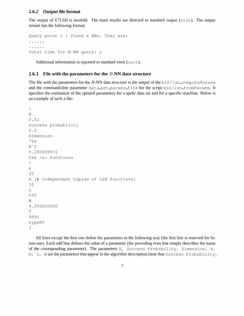
2.6.3 File with the parameters for theR-NN data structure

The file with the parameters for theR-NN data structure is the output of thebin/lsh computeParamsand the command-line parameterdata set params file for the scriptbin/lsh fromParams . Itspecifies the estimation of the optimal parameters for a spefic data set and for a specific machine. Below isan example of such a file:

1R0.53Success probability0.9Dimension784Rˆ20.280899972Use <u> functions1k20m [# independent tuples of LSH functions]35L595W4.000000000T9991typeHT3

All lines except the first one define the parameters in the following way (the first line is reserved for fu-ture use). Each odd line defines the value of a parameter (the preceding even line simply describes the nameof the corresponding parameter). The parametersR, Success Probability, Dimension, k,m, L, W are the parameters that appear in the algorithm description(note thatSuccess Probability,

7

k, m, L are interrelated values as described in 3.5.1). The parameter Rˆ2 is equal toR2. The parameterT is reserved for specifying how many points to look through before the query algorithm stops, but thisparameter is not implemented yet (and therefore is set ton).

2.6.4 The remainder of the parameter file

Note: understanding of the description below requires familarity with the algorithm of Chapter 3.The parameter “Use <u> functions ” signals whether to use the originalg functions (each of the

L functionsgi is ak-tuple of LSH functions; allkL LSH functions are independent) or whether to useg’sthat are not totally independent (as described in the section 3.4.1). If the value of the parameter is 0, originalg’s are used andL = m; if the value is 1, the modifiedg’s are used andL = m · (m − 1)/2.

The parametertypeHT defines the type of the hash table used for storing the bucketscontaining dataset points. Currently, values of 0 and 3 are supported, but wesuggest to use the value 3. (Refering to thehash table types described in the section 3.6, the value 0 corresponds to the linked-list version of the hashtables, and the value 3 – to the hash tables with hybrid storage arrayY .)

8

Chapter 3

Algorithm description

In this chapter, we describe first the general locality-sensitive hashing algorithm (as in [2] but with slightmodifications). Next, we gradually add more details of the algorithm as well as the optimizations in ourimplementation.

3.1 Notations

We useldp to denote thed-dimensional real spaceRd under thelp norm. For any pointv ∈ Rd, the notation||v||p represents thelp norm of the vectorv, that is

||v||p = (d∑

i=1

vpi )

1/p

In particular||v|| = ||v||2 is the Euclidean norm.Let the data setP be a finite subset ofRd, and letn = |P|. A point q will usually stand for the query

point; the query point is any point fromRd. Pointsv, u will usually stand for some points in the data setP.The ball of radiusr centered atv is denoted byB(v, r). For a query pointq, we call v an R-near

neighbor (or simply a near neighbor) ifv ∈ B(q,R).

3.2 Generic locality-sensitive hashing scheme

To solve theR-NN problem, we use the technique of Locality Sensitive Hashing or LSH [4, 3]. For a domainS of points, the LSH family is defined as:

Definition 1 A family H = {h : S → U} is called locality-sensitive, if for any q, the function p(t) =PrH[h(q) = h(v) : ||q − v|| = t] is strictly decreasing in t. That is, the probability of collision of points qand v is decreasing with the distance between them.

Thus, if we consider any pointsq, v, u, with v ∈ B(q,R) andu 6∈ B(q,R), then we have thatp(||q −v||) > p(||q − u||). Intuitively we could hash the points fromP into some domainU , and then at the querytime compute the hash ofq and consider only the points with whichq collides.

However, to achieve the desired running time, we need to amplify the gap between the collision probabil-ities for the range[0, R] (where theR-near neighbors lie) and the range(R,∞). For this purpose we concate-nate several functionsh ∈ H. In particular, fork specified later, define a function familyG = {g : S → Uk}

9

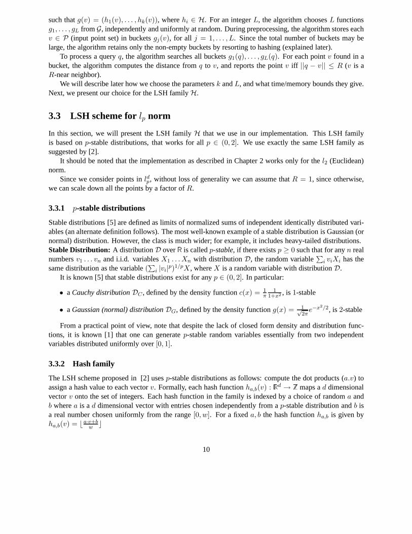
such thatg(v) = (h1(v), . . . , hk(v)), wherehi ∈ H. For an integerL, the algorithm choosesL functionsg1, . . . , gL fromG, independently and uniformly at random. During preprocessing, the algorithm stores eachv ∈ P (input point set) in bucketsgj(v), for all j = 1, . . . , L. Since the total number of buckets may belarge, the algorithm retains only the non-empty buckets by resorting to hashing (explained later).

To process a queryq, the algorithm searches all bucketsg1(q), . . . , gL(q). For each pointv found in abucket, the algorithm computes the distance fromq to v, and reports the pointv iff ||q − v|| ≤ R (v is aR-near neighbor).

We will describe later how we choose the parametersk andL, and what time/memory bounds they give.Next, we present our choice for the LSH familyH.

3.3 LSH scheme forlp norm

In this section, we will present the LSH familyH that we use in our implementation. This LSH familyis based onp-stable distributions, that works for allp ∈ (0, 2]. We use exactly the same LSH family assuggested by [2].

It should be noted that the implementation as described in Chapter 2 works only for thel2 (Euclidean)norm.

Since we consider points inldp, without loss of generality we can assume thatR = 1, since otherwise,we can scale down all the points by a factor ofR.

3.3.1 p-stable distributions

Stable distributions [5] are defined as limits of normalizedsums of independent identically distributed vari-ables (an alternate definition follows). The most well-known example of a stable distribution is Gaussian (ornormal) distribution. However, the class is much wider; forexample, it includes heavy-tailed distributions.Stable Distribution: A distributionD overR is calledp-stable, if there existsp ≥ 0 such that for anyn realnumbersv1 . . . vn and i.i.d. variablesX1 . . . Xn with distributionD, the random variable

∑

i viXi has thesame distribution as the variable(

∑

i |vi|p)1/pX, whereX is a random variable with distributionD.It is known [5] that stable distributions exist for anyp ∈ (0, 2]. In particular:

• a Cauchy distribution DC , defined by the density functionc(x) = 1π

11+x2 , is 1-stable

• a Gaussian (normal) distribution DG, defined by the density functiong(x) = 1√2π

e−x2/2, is 2-stable

From a practical point of view, note that despite the lack of closed form density and distribution func-tions, it is known [1] that one can generatep-stable random variables essentially from two independentvariables distributed uniformly over[0, 1].

3.3.2 Hash family

The LSH scheme proposed in [2] usesp-stable distributions as follows: compute the dot products(a.v) toassign a hash value to each vectorv. Formally, each hash functionha,b(v) : Rd → Z maps ad dimensionalvectorv onto the set of integers. Each hash function in the family is indexed by a choice of randoma andb wherea is ad dimensional vector with entries chosen independently froma p-stable distribution andb isa real number chosen uniformly from the range[0, w]. For a fixeda, b the hash functionha,b is given byha,b(v) = ⌊a·v+b

w ⌋

10

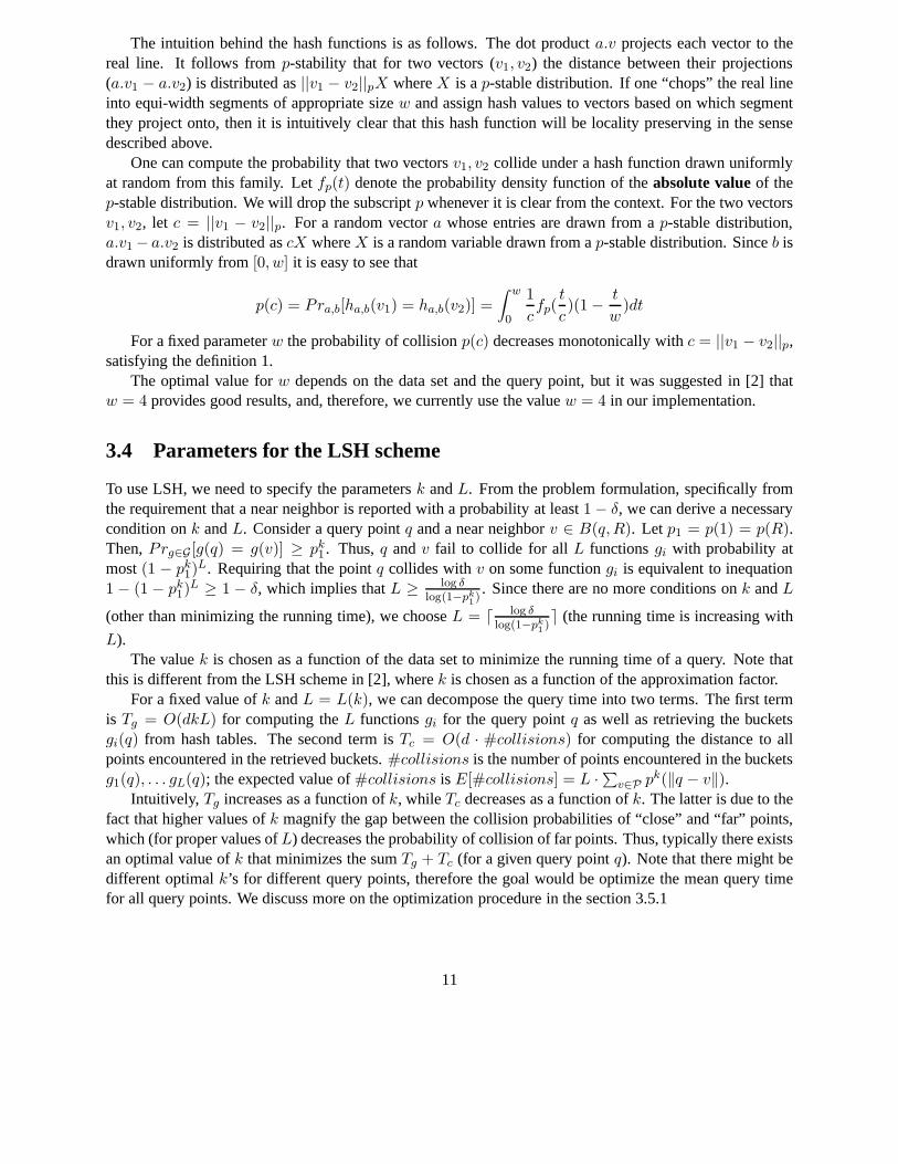
The intuition behind the hash functions is as follows. The dot producta.v projects each vector to thereal line. It follows fromp-stability that for two vectors (v1, v2) the distance between their projections(a.v1 − a.v2) is distributed as||v1 − v2||pX whereX is ap-stable distribution. If one “chops” the real lineinto equi-width segments of appropriate sizew and assign hash values to vectors based on which segmentthey project onto, then it is intuitively clear that this hash function will be locality preserving in the sensedescribed above.

One can compute the probability that two vectorsv1, v2 collide under a hash function drawn uniformlyat random from this family. Letfp(t) denote the probability density function of theabsolute valueof thep-stable distribution. We will drop the subscriptp whenever it is clear from the context. For the two vectorsv1, v2, let c = ||v1 − v2||p. For a random vectora whose entries are drawn from ap-stable distribution,a.v1 − a.v2 is distributed ascX whereX is a random variable drawn from ap-stable distribution. Sinceb isdrawn uniformly from[0, w] it is easy to see that

p(c) = Pra,b[ha,b(v1) = ha,b(v2)] =

∫ w

0

1

cfp(

t

c)(1 − t

w)dt

For a fixed parameterw the probability of collisionp(c) decreases monotonically withc = ||v1 − v2||p,satisfying the definition 1.

The optimal value forw depends on the data set and the query point, but it was suggested in [2] thatw = 4 provides good results, and, therefore, we currently use thevaluew = 4 in our implementation.

3.4 Parameters for the LSH scheme

To use LSH, we need to specify the parametersk andL. From the problem formulation, specifically fromthe requirement that a near neighbor is reported with a probability at least1 − δ, we can derive a necessarycondition onk andL. Consider a query pointq and a near neighborv ∈ B(q,R). Let p1 = p(1) = p(R).Then,Prg∈G [g(q) = g(v)] ≥ pk

1 . Thus,q andv fail to collide for all L functionsgi with probability atmost(1 − pk

1)L. Requiring that the pointq collides withv on some functiongi is equivalent to inequation

1 − (1 − pk1)

L ≥ 1 − δ, which implies thatL ≥ log δlog(1−pk

1). Since there are no more conditions onk andL

(other than minimizing the running time), we chooseL = ⌈ log δlog(1−pk

1)⌉ (the running time is increasing with

L).The valuek is chosen as a function of the data set to minimize the runningtime of a query. Note that

this is different from the LSH scheme in [2], wherek is chosen as a function of the approximation factor.For a fixed value ofk andL = L(k), we can decompose the query time into two terms. The first term

is Tg = O(dkL) for computing theL functionsgi for the query pointq as well as retrieving the bucketsgi(q) from hash tables. The second term isTc = O(d · #collisions) for computing the distance to allpoints encountered in the retrieved buckets.#collisions is the number of points encountered in the bucketsg1(q), . . . gL(q); the expected value of#collisions is E[#collisions] = L ·∑v∈P pk(‖q − v‖).

Intuitively, Tg increases as a function ofk, while Tc decreases as a function ofk. The latter is due to thefact that higher values ofk magnify the gap between the collision probabilities of “close” and “far” points,which (for proper values ofL) decreases the probability of collision of far points. Thus, typically there existsan optimal value ofk that minimizes the sumTg + Tc (for a given query pointq). Note that there might bedifferent optimalk’s for different query points, therefore the goal would be optimize the mean query timefor all query points. We discuss more on the optimization procedure in the section 3.5.1

11

3.4.1 Faster computation of hash functions

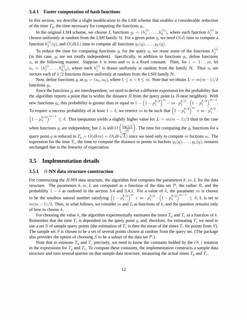
In this section, we describe a slight modification to the LSH scheme that enables a considerable reductionof the timeTg, the time necessary for computing the functionsgi.

In the original LSH scheme, we chooseL functionsgi = (h(i)1 , . . . , h

(i)k ), where each functionh(i)

j ischosen uniformly at random from the LSH familyH. For a given pointq, we needO(d) time to compute a

functionh(i)j (q), andO(dkL) time to compute all functionsg1(q), . . . , gL(q).

To reduce the time for computing functionsgi for the queryq, we reuse some of the functionsh(i)j

(in this case,gi are not totally independent). Specifically, in addition to functionsgi, define functionsui in the following manner. Supposek is even andm is a fixed constant. Then, fori = 1 . . . m, letui = (h

(i)1 , . . . , h

(i)k/2), where eachh(i)

j is drawn uniformly at random from the familyH. Thusui arevectors each ofk/2 functions drawn uniformly at random from the LSH familyH.

Now, define functionsgi asgi = (ua, ub), where1 ≤ a < b ≤ m. Note that we obtainL = m(m−1)/2functionsgi.

Since the functionsgi are interdependent, we need to derive a different expression for the probability thatthe algorithm reports a point that is within the distanceR from the query point (aR-near neighbor). With

new functionsgi, this probability is greater than or equal to1 −(

1 − pk/21

)m− m · pk/2

1 ·(

1 − pk/21

)m−1.

To require a success probability of at least1 − δ, we restrictm to be such that(

1 − pk/21

)m+ m · pk/2

1 ·(

1 − pk/21

)m−1≤ δ. This inequation yields a slightly higher value forL = m(m − 1)/2 than in the case

when functionsgi are independent, butL is still O(

log 1/δ

pk1

)

. The time for computing thegi functions for a

query pointq is reduced toTg = O(dkm) = O(dk√

L) since we need only to computem fuctionsui. Theexpression for the timeTc, the time to compute the distance to points in bucketsg1(q), . . . , gL(q), remainsunchanged due to the linearity of expectation.

3.5 Implementation details

3.5.1 R-NN data structure construction

For constructing theR-NN data structure, the algorithm first computes the parametersk,m,L for the datastructure. The parametersk,m,L are computed as a function of the data setP, the radiusR, and theprobability 1 − δ as outlined in the section 3.4 and 3.4.1. For a value ofk, the parameterm is chosen

to be the smallest natural number satisfying(

1 − pk/21

)m+ m · p

k/21 ·

(

1 − pk/21

)m−1≤ δ; L is set to

m(m − 1)/2. Thus, in what follows, we considerm andL as functions ofk, and the question remains onlyof how to choosek.

For choosing the valuek, the algorithm experimentally estimates the timesTg andTc as a function ofk.Remember that the timeTc is dependent on the query pointq, and, therefore, for estimatingTc we need touse a setS of sample query points (the estimation ofTc is then the mean of the timesTc for points fromS).The sample setS is chosen to be a set of several points chosen at random from the query set. (The packagealso provides the option of choosingS to be a subset of the data setP.)

Note that to estimateTg andTc precisely, we need to know the constants hidded by theO(·) notationin the expressions forTg andTc. To compute these constants, the implementation constructs a sample datastructure and runs several queries on that sample data structure, measuring the actual timesTg andTc.

12

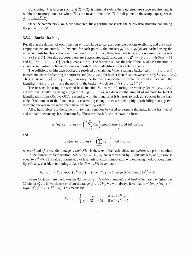
Concluding,k is chosen such thatTc + Tg is minimal (while the data structure space requirement iswithin the memory bounds), whereTc is the mean of the timesTc for all points in the sample query setS:

Tc =

∑

q∈STc(q)

|S| .Once the parametersk,m,L are computed, the algorithm constructs theR-NN data structure containing

the points fromP.

3.5.2 Bucket hashing

Recall that the domain of each functiongi is too large to store all possible buckets explicitly, and only non-empty buckets are stored. To this end, for each pointv, the bucketsg1(v), . . . gL(v) are hashed using theuniversal hash functions. For each functiongi, i = 1 . . . L, there is a hash tableHi containing the buckets{gi(v) | v ∈ P}. For this purpose, there are 2 associated hash functionsh1 : Zk → {0, . . . , tableSize − 1}andh2 : Zk → {0, . . . , C} (eachgi maps toZk). The functionh1 has the role of the usual hash function inan universal hashing scheme. The second hash function identifies the buckets in chains.

The collisions within each bucket are resolved by chaining.When storing a bucketgi(v) = (x1, . . . xk)in its chain, instead of storing the entire vector(x1, . . . xk) for bucket identification, we store onlyh2(x1, . . . xk).Thus, a bucketgi(v) = (x1, . . . xk) has only the following associated information stored in itschain: theidentifierh2(x1, . . . , xk), and the points in the bucket, which areg−1

i (x1, . . . xk) ∩ P.The reasons for using the second hash functionh2 instead of storing the valuegi(v) = (x1, . . . xk)

are twofold. Firstly, by using a fingerprinth2(x1, . . . xk), we decrease the amount of memory for bucketidentification fromO(k) to O(1). Secondly, with the fingerprint it is faster to look up a bucket in the hashtable. The domain of the functionh2 is chosen big enough to ensure with a high probability that any twodifferent buckets in the same chain have differenth2 values.

All L hash tables use the same primary hash functionh1 (used to dermine the index in the hash table)and the same secondary hash functionh2. These two hash functions have the form

h1(a1, a2, . . . , ak) =

((

k∑

i=1

r′iai

)

modprime

)

modtableSize,

and

h2(a1, a2, . . . , ak) =

(

k∑

i=1

r′′i ai

)

modprime,

wherer′i andr′′i are random integers,tableSize is the size of the hash tables, andprime is a prime number.In the current implementation,tableSize = |P|, ai are represented by 32-bit integers, andprime is

equal to232−5. This value of prime allows fast hash function computation without using modulo operations.Specifically, consider computingh2(a1) for k = 1. We have that:

h2(a1) =(

r′′1a1)

mod(

232 − 5)

=(

low[

r′′1a1]

+ 5 · high[

r′′1a1])

mod(232 − 5)

wherelow[r′′1a1] are the low-order 32 bits ofr′′1a1 (a 64-bit number), andhigh[r′′1a1] are the high-order32 bits ofr′′1a1. If we chooser′′i from the range[1, . . . 229], we will always have thatα = low [r′′1a1] + 5 ·high [r′′1a1] < 2 ·

(

232 − 5)

. This means that

h2(a1) =

{

α , if α < 232 − 5α −

(

232 − 5)

, if α ≥ 232 − 5

13

Fork > 1, we compute progressively the sum(

∑ki=1 r′′i ai

)

modprime keeping always the partial sum

modulo(

232 − 5)

using the same principle as the one above. Note that the rangeof the functionh2 thusbecomes{1, . . . 232 − 6}.

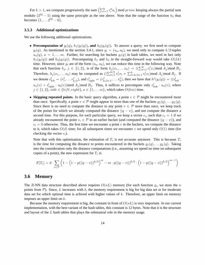
3.5.3 Additional optimizations

We use the following additional optimizations.

• Precomputation of gi(q), h1(gi(q)), and h2(gi(q)). To answer a query, we first need to computegi(q). As mentioned in the section 3.4.1, sincegi = (ua, ub), we need only to computek/2-tuplesua(q), a = 1, . . . m. Further, for searching for bucketsgi(q) in hash tables, we need in fact onlyh1(gi(q)) andh2(gi(q)). Precomputingh1 andh2 in the straight-forward way would takeO(Lk)time. However, sincegi are of the form(ua, ub), we can reduce this time in the following way. Notethat each functionhj , j ∈ {1, 2}, is of the formhj(x1, . . . xk) = ((

∑kt=1 rj

i xi)modAj)modBj.

Therefore,hj(x1, . . . xk) may be computed as((∑k/2

t=1 rjt xt +

∑kt=k/2+1 rj

t xt)modAj)modBj . If

we denoterjleft = (rj1, . . . r

jk/2), andrjright = (rj

k/2+1, . . . rjk), then we have thathj(gi(q)) = ((rjleft ·

ua(v) + rjright · ub(v))modAj)modBj . Thus, it suffices to precompute onlyrjside · ua(v), wherej ∈ {1, 2}, side ∈ {left, right}, a ∈ {1, . . . m}, which takesO(km) time.

• Skipping repeated points. In the basic query algorithm, a pointv ∈ P might be encountered morethan once. Specifically, a pointv ∈ P might appear in more than one of the bucketsg1(q), . . . gL(q).Since there is no need to compute the distance to any pointv ∈ P more than once, we keep trackof the points for which we already computed the distance||q − v||, and not compute the distance asecond time. For this purpose, for each particular query, wekeep a vectorei, such thatei = 1 if wealready encountered the pointvi ∈ P in an earlier bucket (and computed the distance||q − v||), andei = 0 otherwise. Thus, the first time we encounter a pointv in the buckets, we compute the distanceto it, which takesO(d) time; for all subsequent times we encounterv we spend onlyO(1) time (forchecking the vectorei).

Note that with this optimization, the estimation ofTc is not accurate anymore. This is becauseTc

is the time for computing the distance to points encounteredin the bucketsg1(q), . . . gL(q). Takinginto the consideration only the distance computations (i.e., assuming we spend no time on subsequentcopies of a point), the new expression forTc is

E[Tc] = d ·∑

v∈P

(

1 −(

1 − p(||q − v||)k/2)m

− m · p(||q − v||)k/2 ·(

1 − p(||q − v||)k/2)m−1

)

3.6 Memory

The R-NN data structure described above requiresO(nL) memory (for each functiongi, we store thenpoints fromP). Since,L increases withk, the memory requirement is big for big data set or for moderatedata set for which optimal time is achived with higher valuesof k. Therefore, an upper limit on memoryimposes an upper limit onk.

Because the memory requirement is big, the constant in frontof O(nL) is very important. In our currentimplementation, with the best variant of the hash tables, this constant is 12 bytes. Note that it is the structureand layout of theL hash tables that plays the substantial role in the memory usage.

14

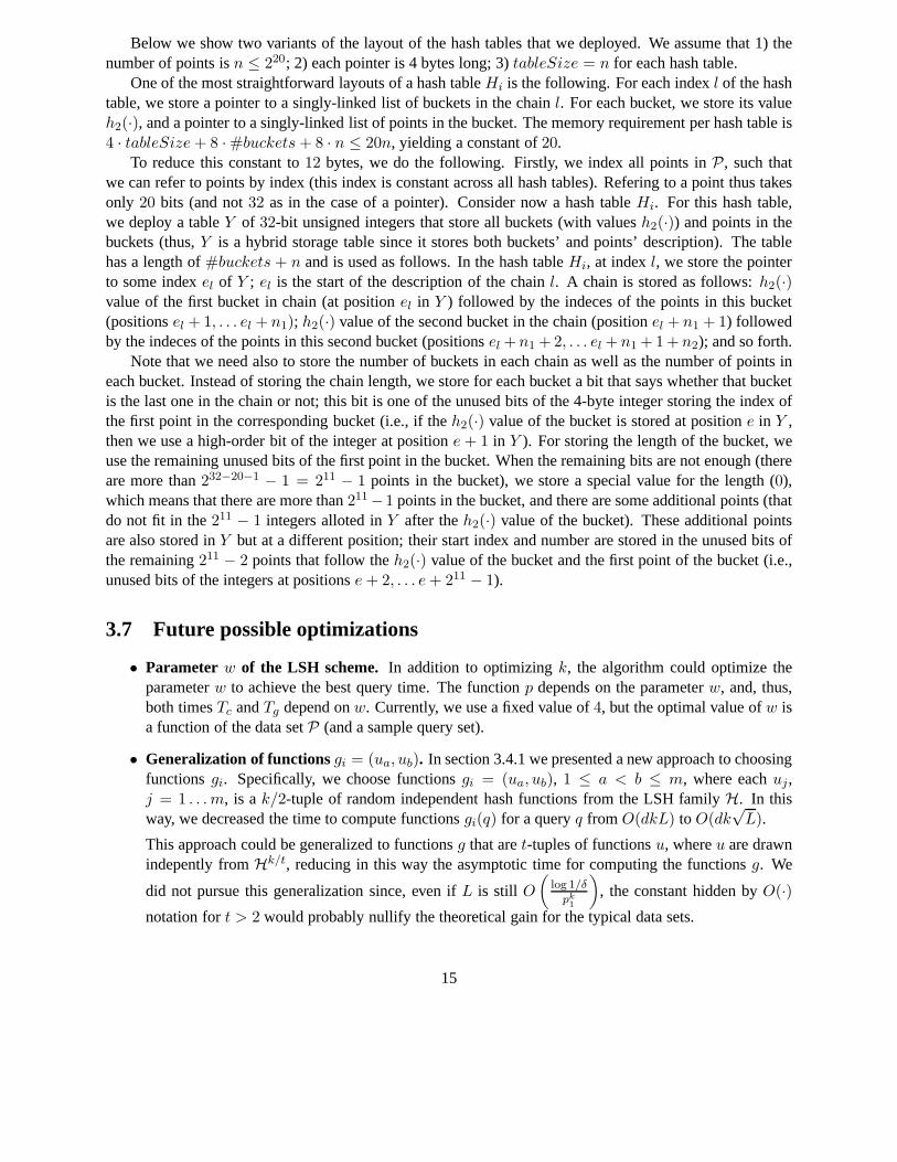
Below we show two variants of the layout of the hash tables that we deployed. We assume that 1) thenumber of points isn ≤ 220; 2) each pointer is 4 bytes long; 3)tableSize = n for each hash table.

One of the most straightforward layouts of a hash tableHi is the following. For each indexl of the hashtable, we store a pointer to a singly-linked list of buckets in the chainl. For each bucket, we store its valueh2(·), and a pointer to a singly-linked list of points in the bucket. The memory requirement per hash table is4 · tableSize + 8 · #buckets + 8 · n ≤ 20n, yielding a constant of20.

To reduce this constant to12 bytes, we do the following. Firstly, we index all points inP, such thatwe can refer to points by index (this index is constant acrossall hash tables). Refering to a point thus takesonly 20 bits (and not32 as in the case of a pointer). Consider now a hash tableHi. For this hash table,we deploy a tableY of 32-bit unsigned integers that store all buckets (with valuesh2(·)) and points in thebuckets (thus,Y is a hybrid storage table since it stores both buckets’ and points’ description). The tablehas a length of#buckets + n and is used as follows. In the hash tableHi, at indexl, we store the pointerto some indexel of Y ; el is the start of the description of the chainl. A chain is stored as follows:h2(·)value of the first bucket in chain (at positionel in Y ) followed by the indeces of the points in this bucket(positionsel + 1, . . . el + n1); h2(·) value of the second bucket in the chain (positionel + n1 + 1) followedby the indeces of the points in this second bucket (positionsel + n1 + 2, . . . el + n1 + 1 + n2); and so forth.

Note that we need also to store the number of buckets in each chain as well as the number of points ineach bucket. Instead of storing the chain length, we store for each bucket a bit that says whether that bucketis the last one in the chain or not; this bit is one of the unusedbits of the 4-byte integer storing the index ofthe first point in the corresponding bucket (i.e., if theh2(·) value of the bucket is stored at positione in Y ,then we use a high-order bit of the integer at positione + 1 in Y ). For storing the length of the bucket, weuse the remaining unused bits of the first point in the bucket.When the remaining bits are not enough (thereare more than232−20−1 − 1 = 211 − 1 points in the bucket), we store a special value for the length(0),which means that there are more than211 −1 points in the bucket, and there are some additional points (thatdo not fit in the211 − 1 integers alloted inY after theh2(·) value of the bucket). These additional pointsare also stored inY but at a different position; their start index and number arestored in the unused bits ofthe remaining211 − 2 points that follow theh2(·) value of the bucket and the first point of the bucket (i.e.,unused bits of the integers at positionse + 2, . . . e + 211 − 1).

3.7 Future possible optimizations

• Parameter w of the LSH scheme. In addition to optimizingk, the algorithm could optimize theparameterw to achieve the best query time. The functionp depends on the parameterw, and, thus,both timesTc andTg depend onw. Currently, we use a fixed value of4, but the optimal value ofw isa function of the data setP (and a sample query set).

• Generalization of functionsgi = (ua, ub). In section 3.4.1 we presented a new approach to choosingfunctionsgi. Specifically, we choose functionsgi = (ua, ub), 1 ≤ a < b ≤ m, where eachuj,j = 1 . . . m, is ak/2-tuple of random independent hash functions from the LSH family H. In thisway, we decreased the time to compute functionsgi(q) for a queryq from O(dkL) to O(dk

√L).

This approach could be generalized to functionsg that aret-tuples of functionsu, whereu are drawnindepently fromHk/t, reducing in this way the asymptotic time for computing the functionsg. We

did not pursue this generalization since, even ifL is still O

(

log 1/δ

pk1

)

, the constant hidden byO(·)notation fort > 2 would probably nullify the theoretical gain for the typicaldata sets.

15

Chapter 4

The E2LSH Code

4.1 Code overview

The core of the E2LSH code is divided into three main components:

• LocalitySensitiveHashing.cpp – contains the implementation of the main LSH-basedR-near neighbor data strucure (except the hashing of the buckets). The main functionality is for con-structing the data structure (given the parameters such ask,m,L), and for answering a query.

• BucketHashing.cpp – contains the implementation of the hash tables for the universal hashingof the buckets. The main functionality is for constructing hash tables, adding new buckets/points toit, and looking-up a bucket.

• SelfTuning.cpp – contains functions for computing the optimal parameters for theR-near neigh-bor data structure. Contains all the functions for estimating the timesTc, Tg (including the functionsfor estimating#collisions).

Additional code making part of the core is contained in the following files:

• Geometry.h – contains the definition for a point (PPointT data type);

• NearNeighbors.cpp ,NearNeighbors.h – contain the functions at the interface of the E2LSHcore (see a more detailed description below);

• Random.cpp , Random.h – contain the pseudo-random number generator;

• BasicDefinitions.h – contains the definitions of general-purpose types (such as, IntT , RealT )and macros (such as the macros for timing operations);

• Utils.cpp , Utils.h – contain some general purpose functions (e.g., copying vectors).

Another important part of the package is the fileLSHMain.cpp , which is a sample code for usingE2LSH. LSHMain.cpp only reads the input files, parses the command line parameters, and calls the cor-responding functions from the package.

The most important data structures are:

16

• RNearNeighborStructureT – the fundamentalR-near neighbor data structure. This structurecontains the parameters used to construct the structure, the description of the functionsgi, the index ofthe points in the structure, as well pointers to theL hash tables for storing the buckets. The structureis defined inLocalitySensitiveHashing.h .

• UHashStructureT – the structure defining a hash table used for hashing the buckets. Collisionsare resolved using chaining as explained in sections 3.5.2 and 3.6. There are 2 main types of hashtables: HT LINKED LIST and HT HYBRID CHAINS (the field typeHT contains the type of thehash table). The typeHT LINKED LIST corresponds to the linked-list version of the hash table, andHT HYBRID CHAINS– to the one with hybrid storage arrayY (see section 3.6 for more details).Each hash table also contains pointers to the descriptions of the functionsh1(·) andh2(·) used for theuniversal hashing. The structure is defined inBucketHashing.h .

• RNNParametersT – a struct containing the parameters necessary for constructing theRNearNeighborStructureT data structure. It is defined inLocalitySensitiveHashing.h .

• PPoint – a struct for storing a point fromP or a query point. This structure contains the coordinatesof the point, the square of the norm of the point, and an index,which can be used by the callee outsidethe E2LSH code (such asLSHMain.cpp ) for identifying the point (for example, it might by theindex of the point in the setP); this index is not used within the core of E2LSH.

4.2 E2LSH Interface

The following are the functions at the interface of E2LSH core code. The first two functions are suffi-cient for constructing theR-NN data structure, and querying it afterwards; they are declared in the fileNearNeighbors.h . The following two functions provide a separation of the estimation of the parameter(such ask,m,L) from the construction of theR-NN data structure itself.

1. To construct theR-NN data structure given as input1 − δ, R, d, and the data setP, one can use thefunction

PRNearNeighborStructTinitSelfTunedRNearNeighborWithDataSet(RealT threshol dR,

RealT successProbability,Int32T nPoints,IntT dimension,PPointT *dataSet,IntT nSampleQueries,PPointT *sampleQueries)

The function will estimate optimal parametersk,m,L, and will construct aR-NN data structure fromthis parameters.

The parameters of the function are the input data of the algorithm: R, 1− δ, n, d, and respectivelyP.The parametersampleQueries represents a set of sample query points – the function optimizesthe parameters of the constructed data structure for the points specified in the setsampleQueries .

17

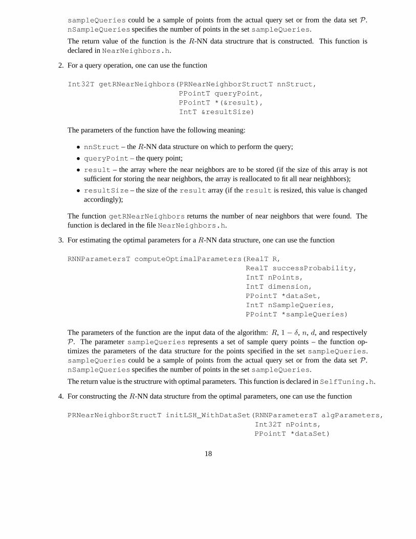
sampleQueries could be a sample of points from the actual query set or from the data setP.nSampleQueries specifies the number of points in the setsampleQueries .

The return value of the function is theR-NN data structrure that is constructed. This function isdeclared inNearNeighbors.h .

2. For a query operation, one can use the function

Int32T getRNearNeighbors(PRNearNeighborStructT nnStru ct,PPointT queryPoint,PPointT *(&result),IntT &resultSize)

The parameters of the function have the following meaning:

• nnStruct – theR-NN data structure on which to perform the query;

• queryPoint – the query point;

• result – the array where the near neighbors are to be stored (if the size of this array is notsufficient for storing the near neighbors, the array is reallocated to fit all near neighhbors);

• resultSize – the size of theresult array (if theresult is resized, this value is changedaccordingly);

The functiongetRNearNeighbors returns the number of near neighbors that were found. Thefunction is declared in the fileNearNeighbors.h .

3. For estimating the optimal parameters for aR-NN data structure, one can use the function

RNNParametersT computeOptimalParameters(RealT R,RealT successProbability,IntT nPoints,IntT dimension,PPointT *dataSet,IntT nSampleQueries,PPointT *sampleQueries)

The parameters of the function are the input data of the algorithm: R, 1 − δ, n, d, and respectivelyP. The parametersampleQueries represents a set of sample query points – the function op-timizes the parameters of the data structure for the points specified in the setsampleQueries .sampleQueries could be a sample of points from the actual query set or from the data setP.nSampleQueries specifies the number of points in the setsampleQueries .

The return value is the structrure with optimal parameters.This function is declared inSelfTuning.h .

4. For constructing theR-NN data structure from the optimal parameters, one can use the function

PRNearNeighborStructT initLSH_WithDataSet(RNNParamet ersT algParameters,Int32T nPoints,PPointT *dataSet)

18

algParameters specify the parameters with which theR-NN data structure will be constructed.

The function returns the constructed data structure. The function is declared inLocalitySensitiveHashing.h .

19

Chapter 5

Frequent Anticipated Questions

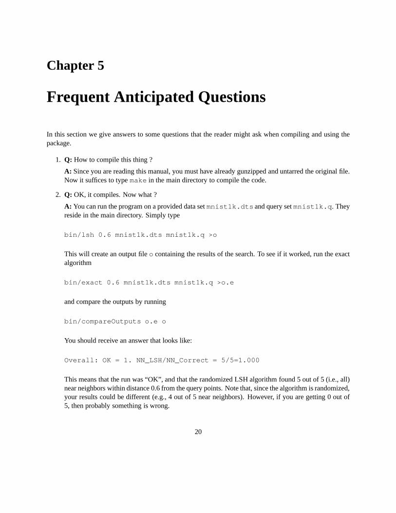
In this section we give answers to some questions that the reader might ask when compiling and using thepackage.

1. Q: How to compile this thing ?

A: Since you are reading this manual, you must have already gunzipped and untarred the original file.Now it suffices to typemake in the main directory to compile the code.

2. Q: OK, it compiles. Now what ?

A: You can run the program on a provided data setmnist1k.dts and query setmnist1k.q . Theyreside in the main directory. Simply type

bin/lsh 0.6 mnist1k.dts mnist1k.q >o

This will create an output fileo containing the results of the search. To see if it worked, runthe exactalgorithm

bin/exact 0.6 mnist1k.dts mnist1k.q >o.e

and compare the outputs by running

bin/compareOutputs o.e o

You should receive an answer that looks like:

Overall: OK = 1. NN_LSH/NN_Correct = 5/5=1.000

This means that the run was “OK”, and that the randomized LSH algorithm found 5 out of 5 (i.e., all)near neighbors within distance 0.6 from the query points. Note that, since the algorithm is randomized,your results could be different (e.g., 4 out of 5 near neighbors). However, if you are getting 0 out of5, then probably something is wrong.

20

3. Q: I ran the code, but it is so slow!

A: If the code is unusually slow, it might mean two things:

• The code uses so much memory that the system starts swapping.This typically degrades theperformance by 3 orders of magnitude, so should be definitelyavoided. To fix it, specify theamount of available (not total) memory in the filebin/mem .

• The search radius you specified is so large that many/most of the data points are reported as nearneighbors. If this is what you want, then the code will not runmuch faster. In fact, you might bebetter off using linear scan instead, since it is simpler andhas less overhead.

Otherwise, try to adjust the search radius so that, on average, there are few near neighbors perquery. You can usebin/exact for experiments, it is likely to be faster than LSH if youperform just a few queries.

21

Bibliography

[1] J. M. Chambers, C. L. Mallows, and B. W. Stuck. A method forsimulating stable random variables.J.Amer. Statist. Assoc., 71:340–344, 1976.

[2] M. Datar, N. Immorlica, P. Indyk, and V. Mirrokni. Locality-sensitive hashing scheme based on p-stabledistributions.DIMACS Workshop on Streaming Data Analysis and Mining, 2003.

[3] A. Gionis, P. Indyk, and R. Motwani. Similarity search inhigh dimensions via hashing.Proceedings ofthe 25th International Conference on Very Large Data Bases (VLDB), 1999.

[4] P. Indyk and R. Motwani. Approximate nearest neighbor: towards removing the curse of dimensionality.Proceedings of the Symposium on Theory of Computing, 1998.

[5] V.M. Zolotarev. One-Dimensional Stable Distributions. Vol. 65 of Translations of Mathematical Mono-graphs, American Mathematical Society, 1986.

22