Problem Set 8 - Solution - math.mit.edumath.mit.edu/classes/18.085/summer2016/pset2016... ·...

18.085: Summer 2016 Due: 3 August 2016 (in class)

Problem Set 8 - Solution

Jonasz Słomka

Unless otherwise specified, you may use MATLAB to assist with computations. Pleaseprovide a print-out of the code used and its output with your assignment.

1. More on relation between Fourier series and Discrete Fourier Transform (DFT).

Let f(x) be a periodic function of period 2π. We can express it as a Fourier series

f(x) =∞∑

k=−∞

ckeikx. (1)

Suppose we want to approximate f(x) by keeping only the first n lowest frequencyamplitudes

f(x) ≈n∑

k=−n

ckeikx. (2)

The number of terms on the rhs is N = 2n+ 1. Let’s sample f(x) at points

xj =2π

Nj j = −n, . . . , 0, . . . n, (3)

that are uniformly distributed over the interval (−π, π), and include the origin.

If we denote the corresponding vector of samples by fj = f(xj), then, at point xj, theapproximation (2) gives

fj =n∑

k=−n

ckωkj, (4)

where ω = e−i2πN . Similarly, we can approximate the exact expression for the Fourier

coefficient ck by the finite sum

ck =1

2π

∫ π

−πf(x)e−ikxdx ≈ 1

2π

n∑j=−n

fjωkj∆x, k = −n, . . . , 0, . . . n. (5)

Since ∆x = 2πN, this is

ck =1

N

n∑j=−n

fjωkj. (6)

We can see that Eq. (6) looks almost like the DFT and Eq. (4) is almost the inverseDFT. What is different is that the zero frequency mode is in the middle, rather thanon the left. We need two steps to exactly recover the usual DFT.

18.085 PSET8 - Solution of 12


First, note that fj and ck are labelled from −n to n while in the definition of DFT wehave labels from 0 to N . Let’s relabel: fk = fk−n and ck = ck−n. If we also change thesummation to run from 0 to N , we get

fj =N−1∑k=0

ckω(k−n)(j−n), ck =

1

N

N−1∑j=0

fjω(k−n)(j−n). (7)

We shift the above expressions by n

fj+n =N−1∑k=0

ckω(k−n)j, ck+n =

1

N

N−1∑j=0

fjωk(j−n). (8)

A small rearrangement gives

ωnj fj+n =N−1∑k=0

ckωkj, ωknck+n =

1

N

N−1∑j=0

fjωkj. (9)

If you remember that, for DFT and its inverse, factor like ωkn in front of ck+n comesfrom the shift of fj by n, fj → fj−n, then you realize that the above formulae are exactlyinverse DFT and DFT, respectively, just with input and output shifted. MATLABhas built in commands to perform these shifts for you. All you need is fftshift()and ifftshift() on top of the usual fft() (DFT) and ifft() (inverse DFT). Thetransforms are

f = fftshift(ifft(ifftshift(N ∗ c))), (10)c = fftshift(fft(ifftshift(f/N))).

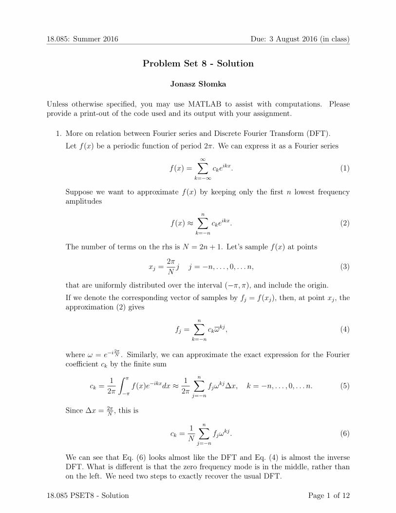
(a) In Problem set 6 you showed that the periodic function f(x) defined by f(x) = xon (−π, π) has Fourier series given by

f(x) = −2∑k=1

(−1)k

ksin(kt). (11)

Convert f(x) into the complex form f =∑∞

k=−∞ ckeikx (find ck).

Answer: Since sin(kt) = eikt−e−ikt2i

, we get

c0 = 0, (12)

ck = i(−1)k

k, k > 0,

ck = −c−k, k < 0.

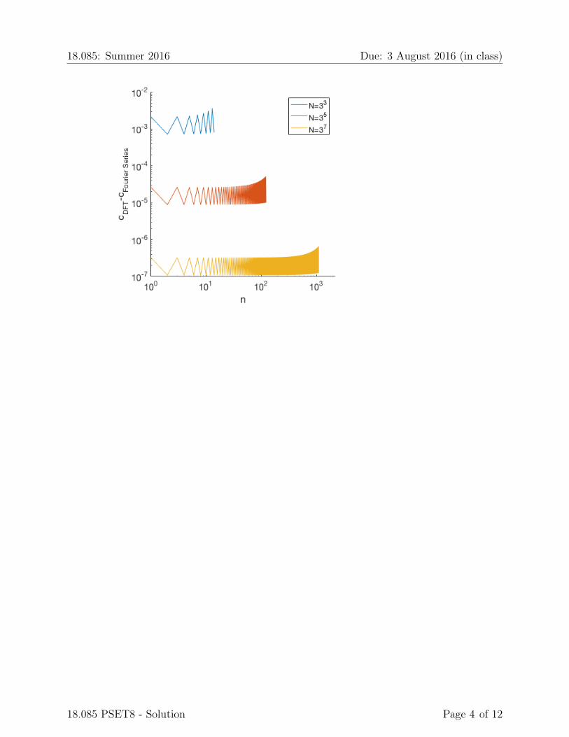
(b) Sample f(x) at the grid points defined by Eq. (3). Do so forN = 2n+1 equal to 33,35 and 37. Convert the samples to the coefficients using c = fftshift(fft(ifftshift(f/N))).Plot the difference between these coefficients and the coefficients of the Fourier



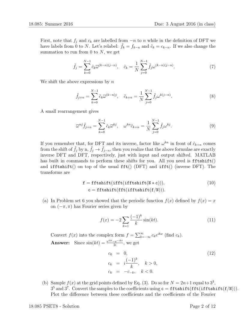
series from (a). Use log-log scale. Comment on the behaviour of the differencefor the three values of N .Answer

Evaluating c = fftshift(fft(ifftshift(f/N))) is like approximating the inte-grals ck = 1

2π

∫ π−π f(x)e−inxdx. The higher the discretization size, the better the

approximation.

(c) In Problem set 7 you showed that the periodic function g(x) defined by g(x) = |x|on (−π, π) has Fourier series given by

g(x) =π

2− 4

π

∞∑n=1,3,5,···

1

n2cos(nx). (13)

Repeat (a) and (b) for g(x).Answer: Since cos(kt) = eikt+e−ikt

2, we get

c0 =π

2, (14)

ck = − 2

π

1

k2, k > 0, k odd,

ck = c−k, k < 0, k odd.



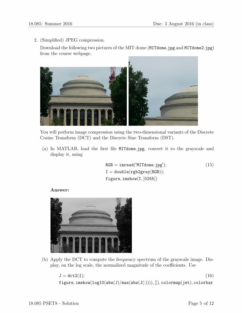
2. (Simplified) JPEG compression.

Download the following two pictures of the MIT dome (MITdome.jpg and MITdome2.jpg)from the course webpage.

You will perform image compression using the two-dimensional variants of the DiscreteCosine Transform (DCT) and the Discrete Sine Transform (DST).

(a) In MATLAB, load the first file MITdome.jpg, convert it to the grayscale anddisplay it, using

RGB = imread(′MITdome.jpg′); (15)I = double(rgb2gray(RGB));

figure, imshow(I, [0255])

Answer:

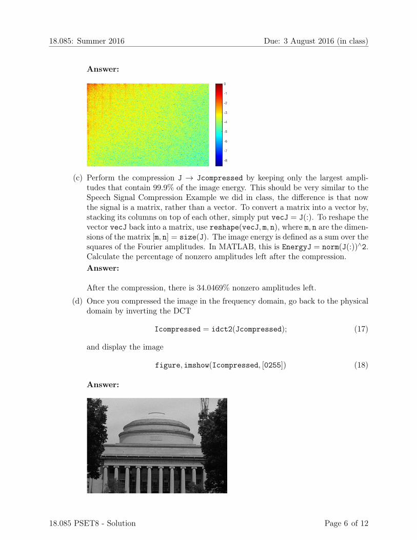
(b) Apply the DCT to compute the frequency spectrum of the grayscale image. Dis-play, on the log scale, the normalized magnitude of the coefficients. Use

J = dct2(I); (16)figure, imshow(log10(abs(J)/max(abs(J(:)))), []), colormap(jet), colorbar



Answer:

(c) Perform the compression J → Jcompressed by keeping only the largest ampli-tudes that contain 99.9% of the image energy. This should be very similar to theSpeech Signal Compression Example we did in class, the difference is that nowthe signal is a matrix, rather than a vector. To convert a matrix into a vector by,stacking its columns on top of each other, simply put vecJ = J(:). To reshape thevector vecJ back into a matrix, use reshape(vecJ, m, n), where m, n are the dimen-sions of the matrix [m, n] = size(J). The image energy is defined as a sum over thesquares of the Fourier amplitudes. In MATLAB, this is EnergyJ = norm(J(:))∧2.Calculate the percentage of nonzero amplitudes left after the compression.Answer:

After the compression, there is 34.0469% nonzero amplitudes left.

(d) Once you compressed the image in the frequency domain, go back to the physicaldomain by inverting the DCT

Icompressed = idct2(Jcompressed); (17)

and display the image

figure, imshow(Icompressed, [0255]) (18)

Answer:



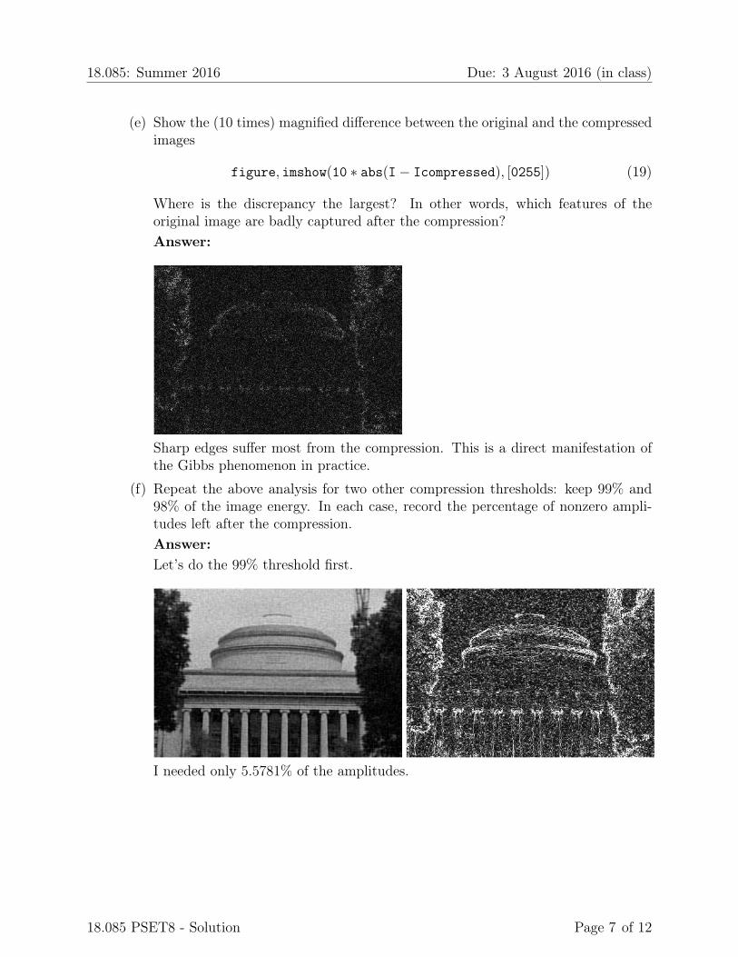
(e) Show the (10 times) magnified difference between the original and the compressedimages

figure, imshow(10 ∗ abs(I− Icompressed), [0255]) (19)

Where is the discrepancy the largest? In other words, which features of theoriginal image are badly captured after the compression?Answer:

Sharp edges suffer most from the compression. This is a direct manifestation ofthe Gibbs phenomenon in practice.

(f) Repeat the above analysis for two other compression thresholds: keep 99% and98% of the image energy. In each case, record the percentage of nonzero ampli-tudes left after the compression.Answer:Let’s do the 99% threshold first.

I needed only 5.5781% of the amplitudes.



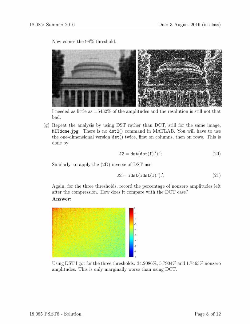
Now comes the 98% threshold.

I needed as little as 1.5432% of the amplitudes and the resolution is still not thatbad.

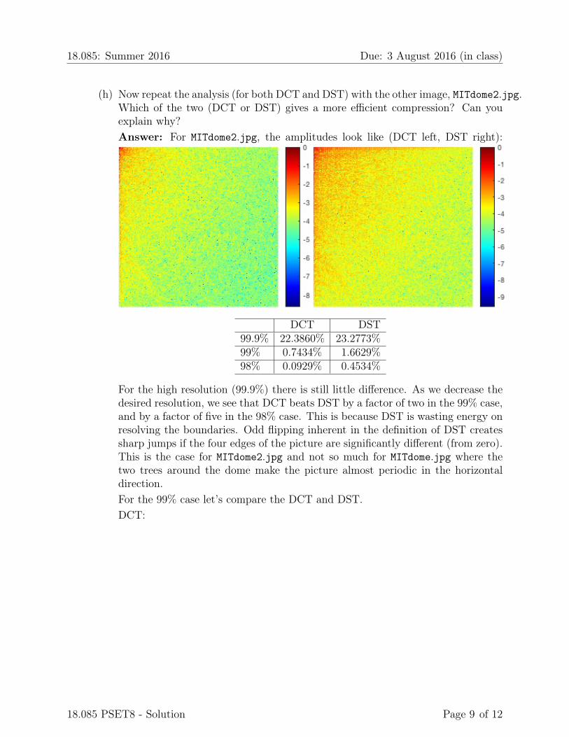
(g) Repeat the analysis by using DST rather than DCT, still for the same image,MITdome.jpg. There is no dst2() command in MATLAB. You will have to usethe one-dimensional version dst() twice, first on columns, then on rows. This isdone by

J2 = dst(dst(I).′).′; (20)

Similarly, to apply the (2D) inverse of DST use

J2 = idst(idst(I).′).′; (21)

Again, for the three thresholds, record the percentage of nonzero amplitudes leftafter the compression. How does it compare with the DCT case?Answer:

Using DST I got for the three thresholds: 34.2086%, 5.7904% and 1.7463% nonzeroamplitudes. This is only marginally worse than using DCT.



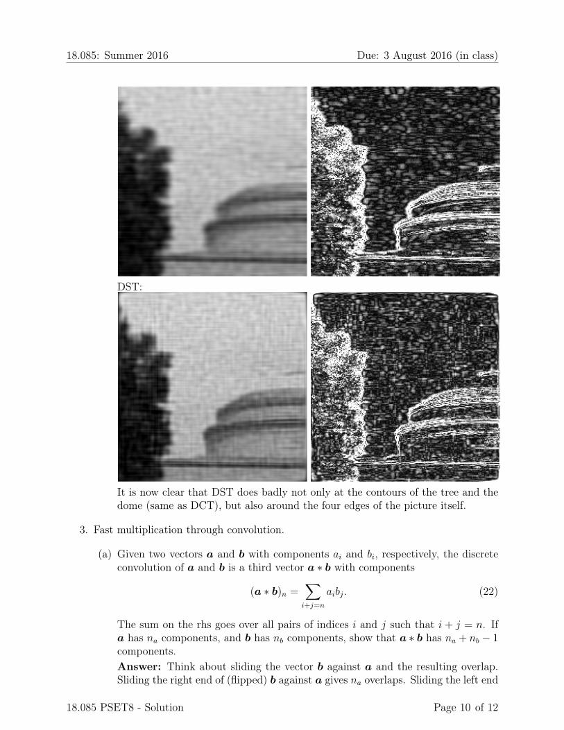
(h) Now repeat the analysis (for both DCT and DST) with the other image, MITdome2.jpg.Which of the two (DCT or DST) gives a more efficient compression? Can youexplain why?Answer: For MITdome2.jpg, the amplitudes look like (DCT left, DST right):

DCT DST99.9% 22.3860% 23.2773%99% 0.7434% 1.6629%98% 0.0929% 0.4534%

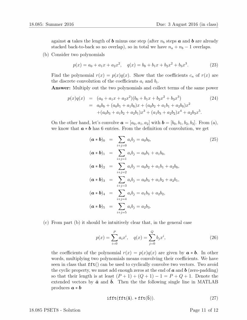
For the high resolution (99.9%) there is still little difference. As we decrease thedesired resolution, we see that DCT beats DST by a factor of two in the 99% case,and by a factor of five in the 98% case. This is because DST is wasting energy onresolving the boundaries. Odd flipping inherent in the definition of DST createssharp jumps if the four edges of the picture are significantly different (from zero).This is the case for MITdome2.jpg and not so much for MITdome.jpg where thetwo trees around the dome make the picture almost periodic in the horizontaldirection.For the 99% case let’s compare the DCT and DST.DCT:



DST:

It is now clear that DST does badly not only at the contours of the tree and thedome (same as DCT), but also around the four edges of the picture itself.

3. Fast multiplication through convolution.

(a) Given two vectors a and b with components ai and bi, respectively, the discreteconvolution of a and b is a third vector a ∗ b with components

(a ∗ b)n =∑i+j=n

aibj. (22)

The sum on the rhs goes over all pairs of indices i and j such that i + j = n. Ifa has na components, and b has nb components, show that a ∗ b has na + nb − 1components.Answer: Think about sliding the vector b against a and the resulting overlap.Sliding the right end of (flipped) b against a gives na overlaps. Sliding the left end



against a takes the length of b minus one step (after nb steps a and b are alreadystacked back-to-back so no overlap), so in total we have na + nb − 1 overlaps.

(b) Consider two polynomials

p(x) = a0 + a1x+ a2x2, q(x) = b0 + b1x+ b2x

2 + b3x3. (23)

Find the polynomial r(x) = p(x)q(x). Show that the coefficients cn of r(x) arethe discrete convolution of the coefficients ai and bi.Answer: Multiply out the two polynomials and collect terms of the same power

p(x)q(x) = (a0 + a1x+ a2x2)(b0 + b1x+ b2x

2 + b3x3) (24)

= a0b0 + (a0b1 + a1b0)x+ (a0b2 + a1b1 + a2b0)x2

+(a0b3 + a1b2 + a2b1)x3 + (a1b3 + a2b2)x

4 + a2b3x5.

On the other hand, let’s convolve a = [a0, a1, a2] with b = [b0, b1, b2, b3]. From (a),we know that a ∗ b has 6 entries. From the definition of convolution, we get

(a ∗ b)0 =∑i+j=0

aibj = a0b0, (25)

(a ∗ b)1 =∑i+j=1

aibj = a0b1 + a1b0,

(a ∗ b)2 =∑i+j=2

aibj = a0b2 + a1b1 + a2b0,

(a ∗ b)3 =∑i+j=3

aibj = a0b3 + a1b2 + a2b1,

(a ∗ b)4 =∑i+j=4

aibj = a1b3 + a2b2,

(a ∗ b)5 =∑i+j=5

aibj = a2b3.

(c) From part (b) it should be intuitively clear that, in the general case

p(x) =P∑i=0

aixi, q(x) =

Q∑j=0

bjxi, (26)

the coefficients of the polynomial r(x) = p(x)q(x) are given by a ∗ b. In otherwords, multiplying two polynomials means convolving their coefficients. We haveseen in class that fft() can be used to cyclically convolve two vectors. Two avoidthe cyclic property, we must add enough zeros at the end of a and b (zero-padding)so that their length is at least (P + 1) + (Q + 1) − 1 = P + Q + 1. Denote theextended vectors by a and b. Then the the following single line in MATLABproduces a ∗ b

ifft(fft(~a). ∗ fft(~b)). (27)



Now suppose you want to multiply two really big numbers, one with 100 and theother with 400 digits. If you want to use Long Multiplication (as in elementaryschool), you would need about 100 × 400 = 40000 operations. Explain how youcan use the above polynomial multiplication-convolution relation and fft() toreduce this number. With fft(), how many operations do you roughly need?Answer: Any number with a finite number of digits in the decimal representationcan be thought of as an evaluation of the polynomial p(x) = a0 +a1x+a2x

2 + . . . ,where ai are the digits of the representation at x = 10. For example, to thenumber 5031, we associate the polynomial

p(x) = 1 + 3x+ 5x3. (28)

Then, of course, 5031 = p(10). Thus, to multiply two large numbers, with thenumber of digits, say na and nb, we can form the two corresponding polynomials(of order na− 1 and nb− 1, respectively). Instead of multiplying the polynomialsdirectly, we can use the zero padding technique and the formula (27). In total,after zero padding, we have three FFTs (of size N = na + nb − 1) and one multi-plication (of size N). The number of operations is roughly (FFT has complexityn log n)

3N logN +N ≈ 3N logN. (29)

This is much slower growth than nanb required when doing the Long Multiplica-tion. For na = 400 and nb = 100, the number of operations is around 9000.


Problem Set 8 - Solution - math.mit.edumath.mit.edu/classes/18.085/summer2016/pset2016... ·...

Documents

Transcript of Problem Set 8 - Solution - math.mit.edumath.mit.edu/classes/18.085/summer2016/pset2016... ·...