DUAL KRIGING: AN EXPLORATORY USE IN … Kriging...Dual Kriging in Economic Metamodeling 249...

The Engineering Economist, 50: 247–271Copyright © 2005 Institute of Industrial EngineersISSN: 0013-791X print / 1547-2701 onlineDOI: 10.1080/00137910500227182

DUAL KRIGING: AN EXPLORATORY USE INECONOMIC METAMODELING

Ravipim Chaveesuk

Program of Agro-Industrial Technology Management, Kasetsart University,Bangkok, Thailand

Alice E. Smith

Department of Industrial and Systems Engineering, Auburn University,Auburn, Alabama, USA

Sensitivity analysis of capital investments can be effectively carried outby employing a metamodel approach and experimental designs. Althoughpolynomial regression metamodels are popular and straightforward, theydo not consider spatial relationships among the data. Dual kriging is anestimation technique that allows the incorporation of spatial correlationinto the interpolation or estimation process and has been used primarilyin geophysical statistical analysis. This article investigates the dual krig-ing approach as an alternative technique to polynomial regression andartificial neural networks for metamodel analysis of capital investments.It is observed that dual kriging shows potential in performing sensitivityanalysis as its accuracy is as good as, or better than, other techniques, and,while model building and interpretation is more complicated than that ofpolynomial regression, it is significantly more straightforward than thatof neural networks. Furthermore, this is the first known work of usingkriging in the field of engineering economics; there may be other usefulapplications such as in cost estimation.

INTRODUCTION

Sensitivity analysis is crucial in deterministic capital investment evaluationsince the estimates of input factors such as the interest rate and amount and

Address correspondence to Alice E. Smith, Department of Industrial and Systems Engi-neering, Auburn University, 207 Dunstan Hall, Auburn University, Auburn, AL 36849, USA.E-mail: [email protected]

248 R. Chaveesuk and A. E. Smith

timing of cash flows used in cash flow analysis are not known with certainty.Not only does sensitivity analysis allow the decision maker to determine therelative effect of changes in the input estimates on the indicated decision,but it can also be used to identify the input factors that are most influentialto the investment decision. The aptness of the final decision depends oncorrectness of the estimates of these significant input factors. In addition,monitoring these factors during implementation of the investment will as-sist the decision maker in taking the right action in a timely manner. Thedrawback of traditional sensitivity analysis, such as one factor at a time andscenario generation, is that interactions among factors are not consideredand it is difficult to derive useful information when three or more factorsare considered.

In order to overcome the problem in traditional sensitivity analysis,Sartori and Smith [18] proposed a polynomial regression metamodel ap-proach. A metamodel is an approximated model of a descriptive modeland is constructed from input-output data generally gathered by design ofexperiments. The concept of a metamodel as defined by Kleijenen [11] canbe explicitly described in terms of the capital investment problem as thefollowing. Let X j denote the value of a factor j influencing the economicmeasure, Y , of the investment under study where {X j | j = 1, 2, . . . , n}.The relationship between the input factors X j and the output or economicmeasure Y can be represented as

Y = f1(X1, X2, . . . , Xn)

This relationship can be generalized to multiple outputs by representingY as a response vector. A metamodel is usually developed separately foreach output Y and only a single output metamodel is considered in thisarticle. A metamodel is an approximation of the investment under studyand may include a subset of the input factors {X j | j = 1, 2, . . . , m}, wherem ≤ n:

Y ′ = f2(X1, X2, . . . , Xm) + εm

The error term, εm , is composed of the effects of any excluded or uniden-tified input factors and the error of fitting the metamodel to the real input-output relationship of the investment.

The regression metamodel is the most popular metamodeling techniqueused in practice. A polynomial regression metamodel for m input factors,(x1, x2, . . . , xm) = x, can be expressed as:

Y =p∑

k=1

βk Zk(x) + εp

Dual Kriging in Economic Metamodeling 249

where there are p power functions Zk(x); e.g., linear, quadratic, cross terms,etc. βk are the regression coefficients, which are calculated from the ob-served pairs of data points via least-squares estimation. ε p is a random errorterm composed of the error of any excluded or unidentified input factorsand the error of fitting the polynomial. This latter component is assumedto distributed according to N (0, σ ).

Sartori and Smith [18] constructed a second-order polynomial regres-sion metamodel from the input factor combinations and the correspondingmeasure of economic value (NPV) that were called for by an experimentaldesign. The validated metamodel was used to carry out sensitivity analysis.It has been shown that this approach was more insightful than traditionalsensitivity analysis. The combination of regression metamodeling and ex-perimental design theory was also used in performing sensitivity analysisof capital investment evaluation by Van Groenendaal [24, 25]. The de-veloped regression metamodels could be used to gain useful informationcontained in the experimental data while the use of experimental designtheory allowed the estimation of interactions between factors, which wasnot possible in traditional sensitivity analysis. Chaveesuk and Smith [3] ap-plied artificial neural networks (ANN) to economic metamodeling, whichshowed potential in certain situations.

Although a polynomial regression metamodel is straightforward to im-plement, it has restricting assumptions of uncorrelated error componentsand absence of multicollinearity. However, correlation might exist amongthe sample data observed from physical or social phenomena. Data close to-gether, in time or in space, are likely to be correlated and should be modeledas such [4]. Kriging is an estimation technique that allows the incorporationof spatial correlation into the interpolation or estimation process. Accord-ingly, it might be an appropriate alternative metamodeling technique torepresent the input-output relationship from cash flow analysis. Barton [1],in his review of metamodeling, includes spatial correlation models or krig-ing models among the most promising metamodeling techniques. Since itsintroduction into the simulation community by Sacks et al. [17], the use ofclassical kriging models for deterministic simulation metamodels has beenlimited [2, 19] due to the complexity of the method and intense computa-tional effort. However, the dual formulation of kriging (dual kriging) wasdeveloped to alleviate the computational problems. Dual kriging has beenadopted in diverse applications including stress analysis [15], a contouringprogram [21], shrinkage analysis [13], modeling of failure behavior forcomposite materials [6–8, 23], modeling and construction of material laws[20, 22], a surrogate for fitness landscape in evolutionary optimization [16],and modeling human radiographic images [5].

This article aims to examine the potential use of dual kriging in per-forming sensitivity analysis of a capital investment evaluation. The theory


of classical kriging and its dual formulation (dual kriging) is reviewed. Amethodology for incorporating a metamodel approach into the sensitiv-ity analysis of capital investment evaluation is then described. The perfor-mance of dual kriging is investigated and compared to that of polynomial re-gression and artificial neural network metamodels through two case studies.

The following notation is used throughout the article:

U (X ) A random function at a specified point XU (Xi ) A set of measurements or computed samples taken

at point Xiu∗(X ) The estimator of U (X )λi A set of weightsE[U (X )] The expected value of U (X )Var[U (X )] The variance of U (X )a(X ) The drift functionb(X ) A stationary fluctuationpl(X ) The basis function of the drift functionσ 2

R The variance of the estimation errorCov[U (X ), u∗(X )] The covariance between U (X ) and u∗(X )ul The Lagrange multipliersCi j The covariance between sample points Xi and X jCi The covariance between sample points Xi and XC(h) The covariance functional and b j The coefficients of the dual kriging model

CLASSICAL KRIGING AND DUAL KRIGING

Kriging is an estimation technique proposed in 1951 by D.G. Krige, a min-ing engineer, for gold deposit evaluations. Similar to polynomial regression,the kriging technique is a BLUE, “Best Linear Unbiased Estimator” of arandom function and is “best” in terms of aiming at minimizing the varianceof estimation error among all linear estimators [15]. Geologists and envi-ronmental engineers have long used kriging to estimate the measurementsor characteristics of hydraulic properties or contaminant concentrations inair, water, or soil in inaccessible or unobserved regions. More recently,its use was extended to the simulation community. Classical kriging (seeJournel & Huijbregts [10] for a thorough treatment) is usually implementedas a local estimation method. That is, its procedure requires the solution ofa new system of equations for each interpolated value. This is obviouslyuntenable for metamodeling.

A global estimation kriging technique called “dual kriging” was devel-oped in 1985 [21] where the kriging system is evaluated only once for thewhole domain by simultaneously using the information provided by all


data points. The development of classical kriging equations and derivationof dual kriging is presented in the following sections (based on Journel andHuijbregts [10], Porier and Tinawi [15], and Trochu [21]).

Theory of Classical Kriging

The purpose of kriging is to estimate the value of a random function U (X )at a specified point or location X , given a set of measurements or computedsamples U (Xi ) taken at location Xi for i = 1, 2, . . . , N . The original theoryof kriging was formulated for dealing with one-, two-, or three-dimensionalproblems, i.e., when X represents the position vector X = x or X = (x , y)or X = (x , y, z). However, it can be generalized to an L dimension problem;i.e., X = (x1, x2, . . . , x L ) as will be done later in this article.

The estimation of U (X ) can be obtained as a linear combination of theobserved data point Xi where i = 1, 2, . . . , N :

u∗(X ) =N∑

i=1

λiU (Xi ) (1)

As a BLUE, a set of weights λi must be determined in such as way that(1) the expected values of U (X ) and u ∗ (X ) are identical; i.e., E[U (X )] =E[u∗(X )], and (2) the variance of the estimation error Var[U (X ) − u∗(X )]is minimized.

In kriging, the random function U (X ) is comprised of the sum of twoterms:

U (X ) = a(X ) + b(X ) (2)

where a(X ) is a drift function representing the average behavior of U (X ) ora(X ) = E[U (X )], and b(X ) is a stationary fluctuation with E[b(X )] = 0.

The kriging system can be derived to minimize the variance of the es-timation error under the constraints of unbiased conditions as follows:From the unbiased condition, E[U (X )] = E[u∗(X )], Equation (1) can beexpressed as

E[U (X )] =N∑

i=1

λi E[U (Xi )] (3)

Since the drift function represents the expected value of U (X ),Equation (3) can be represented by

a(X ) =N∑

i=1

λi a(Xi ) (4)


Usually, the drift function is built up from M basis functions, pl(X ), l = 1,2, . . . , M and the conditions of unbiased become

pl(X ) =N∑

i=1

λi pl(Xi ), l = 1, 2, . . . , M (5)

The variance of the estimation error is calculated as follows

Var[U (X ) − u∗(X )] = σ 2R = Var[U (X )] − 2Cov[U (X ), u∗(X )]

+ Var[u∗(X )]

with Var[U (X )] = σ 2U (X )

Cov[U (X ), u∗(X )] = Cov

{[N∑

i=1

λiU (Xi )

], U (X )

}

=N∑

i=1

λi Cov[U (X ), U (Xi )]

Var[u∗(X )] = Var

[N∑

i=1

λiU (Xi )

]

=N∑

i=1

N∑j=1

λiλ j Cov[U (Xi ), U (X j )]

Combining these three terms, the variance of estimation error can beexpressed as

σ 2R = σ 2

U (X ) − 2N∑

i=1

λi Cov[U (X ), U (Xi )]

+N∑

i=1

N∑j=1

λiλ j Cov[U (Xi ), U (X j )] (6)

This error variance is minimized subject to M unbiased conditions in(5). The constrained minimization problem is converted to an unconstrainedone by introducing M Lagrange multipliers, µl , l = 1, 2, . . . , M , associatedwith the constraints. The solution is then characterized by a linear system


of N + M equations in N + M unknowns λ1, . . . , λN and µ1, . . . , µM :

N∑j=1

λ j Cov[U (Xi ), U (X j )] +M∑

l=1

µl pl(Xi ) = Cov[U (X ), U (X j )],

i=1, 2, . . . , NN∑

j=1

λ j pl(X j ) = pl(X ), l = 1, 2, . . . , M.

(7)

This system is called the “kriging system” and can be written in matrixform

C11 · · · C1N p1(X1) · · · pM (X1)...

. . ....

.... . .

...CN1 · · · CNN p1(X N ) · · · pM (X N )

p1(X1) · · · p1(X N ) 0 · · · 0...

. . ....

.... . .

...pM (X1) · · · pM (X N ) 0 · · · 0

·

λ1

...λN

µ1

...µM

=

C1

...CN

p1(X )...

pM (X )

(8)

where Ci j denotes the covariance between sample points Xi and X j ,or Cov[U (Xi ), U (X j )], and Ci is the covariance between sample pointsXi and a point X , or Cov[U (X ), U (Xi )], in which the value of U (X )is to be estimated. Solving this system yields the optimal values of theλi , i = 1, 2, . . . , N , at the point X .

Dual Formulation of Kriging

The kriging system of Equation (8) depends on the covariance betweenthe sample point Xi and the point X . That is, the solution of system λidepends on point X . Therefore, a new kriging system would be neededfor each estimated value. The dual formulation of kriging was developedto provide independent λi thereby eliminating this limitation. Dual krigingcan be formulated from Equation (8) as follows. When the matrix in system


(8) is inverted, the following expression is obtained:

λ1

...λN

−µ1

...µM

=

|Q | R

|− − − + − − −

|RT | S

|

·

C1

...CN

−p1(X )

...pM (X )

(9)

By substituting this solution into Equation (1), the estimated value u∗(X )can be expressed as:

u∗(X ) = [U (X1) · · · U (X N )] · Q ·

C1

...CN

+ [U (X1) · · · U (X N )] · R ·

p1(X )...

pM (X )

(10)

Using the symmetry of the kriging matrix, a new set of coefficients isdefined as:

b1

...bN

= Q ·

U (X1)...

U (X N )

,

a1

...aM

= RT ·

U (X1)...

U (X N )

(11)

and Equation (10) becomes

u∗(X ) =N∑

j=1

b j C j +M∑

l=1

al pl(X ) (12)


Equation (12) is called dual kriging. The coefficients al , l = 1, . . . , Mand b j , j = 1, . . . , N can be written in matrix form as:

b1

...bN

−a1

...aM

=

|Q | A

|− − − + − − −

|RT | B

|

·

U (X1)...

U (X N )−0...0

(13)

where the matrices A and B are arbitrary. By choosing A = R and B = S,the matrix of Equation (9), which is the inverse kriging matrix, appearsagain in Equation (13). Therefore, the coefficients als and b j s are solutionsof

|Ci j | pl(Xi )

|− − − + − − −

|pl(X j ) | 0

|

·

b1

...bN

−a1

...aM

=

U (X1)...

U (X N )

0...0

(14)

This system of linear equations along with the dual kriging model inEquation (12) comprise the dual formulation of kriging.

The Drift Function and the Covariance Functions

According to Journel and Huijbregts [10], a polynomial drift function isnormally used in geostatistics applications. This can be a complete polyno-mial of order k (k dimensions) composed of all possible subsets of variablesof size 1 to k. For example, an order three basis is expressed as:

a(x) = a0 +L∑

i=1

ai xi +L∑

i=1

L∑j=i

ai j xi x j +L∑

i=1

L∑j=i

L∑k= j

ai jk xi x j xk (15)


Dual kriging also requires the knowledge of the covariance betweentwo points or locations. The covariance between two points or locations isassumed to depend only on the Euclidean distance h between Xi and X j ,(and not on the particular positions Xi or X j ) and is represented by C(h).Usually, the covariance function decreases from a maximum at C(0) sincethe degree of correlation between two locations decreases as the distanceh between them increases [10]. Ratle [16] summarizes two approaches forobtaining the covariance. The first approach is to use an arbitrary theoreti-cal covariance function. These functions are called shape functions ratherthan covariance functions since they have no relationship to the actualcovariance. Kriging under these conditions is considered to be an exactinterpolator. The other approach is to use the estimation of an experimentalcovariance function from the observed data. Under this condition, krigingis employed as an estimator. However, it is difficult to estimate a covari-ance function from the experimental data because it requires the knowledgeof the unknown mean. Consequently, only theoretical covariance will beconsidered in this article.

Ratle [16] has described three common theoretical covariance functions.The first is the pure nugget effect which is the limiting case where thefluctuations around the samples are assumed to be insignificant. This modelis appropriate for noisy data as well as for problems where only a roughestimate of the solution is required. The pure nugget effect covariance iswritten as:

C(h) ={

1 if h = 0;0 otherwise.

(16)

Under the pure nugget effect, there is no correlation between two pointsregardless of distance h. The kriging model does not pass through all ofthe data points and it reduces to a simple polynomial regression on the driftfunction basis.

The other two functions use the notion of distance of influence as in-troduced by Trochu [21]. The models assume that the correlation or actualcovariance between two very distance points is negligible or zero; that is,C(h) = 0 if h > d, where d is a predefined threshold. The first function islinear. It assumes that the covariance decreases linearly from a maximalvalue at h = 0 to zero at h = d. The linear covariance is expressed as:

C(h) ={

1 − h/d if h < d;0 otherwise. (17)

The other function is cubic. This ensures continuity by imposing the nullityof the first derivative of C(h) at the points h = 0 and h = d. Two other


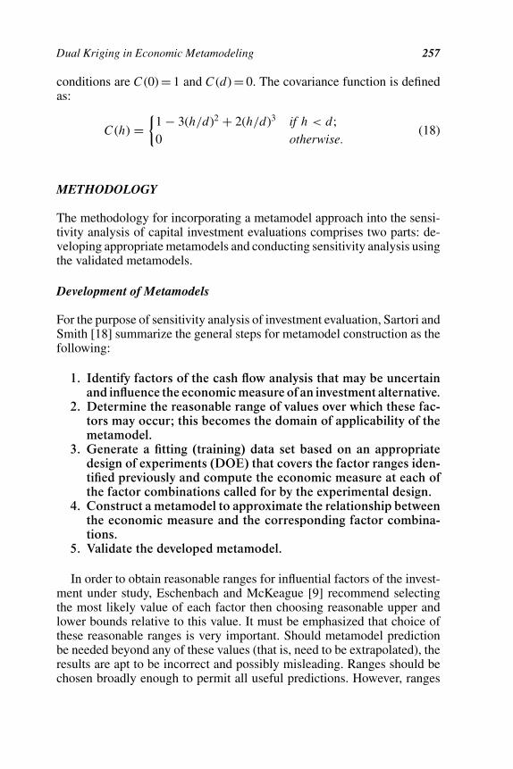
conditions are C(0) = 1 and C(d) = 0. The covariance function is definedas:

C(h) ={

1 − 3(h/d)2 + 2(h/d)3 if h < d;0 otherwise.

(18)

METHODOLOGY

The methodology for incorporating a metamodel approach into the sensi-tivity analysis of capital investment evaluations comprises two parts: de-veloping appropriate metamodels and conducting sensitivity analysis usingthe validated metamodels.

Development of Metamodels

For the purpose of sensitivity analysis of investment evaluation, Sartori andSmith [18] summarize the general steps for metamodel construction as thefollowing:

1. Identify factors of the cash flow analysis that may be uncertainand influence the economic measure of an investment alternative.

2. Determine the reasonable range of values over which these fac-tors may occur; this becomes the domain of applicability of themetamodel.

3. Generate a fitting (training) data set based on an appropriatedesign of experiments (DOE) that covers the factor ranges iden-tified previously and compute the economic measure at each ofthe factor combinations called for by the experimental design.

4. Construct a metamodel to approximate the relationship betweenthe economic measure and the corresponding factor combina-tions.

5. Validate the developed metamodel.

In order to obtain reasonable ranges for influential factors of the invest-ment under study, Eschenbach and McKeague [9] recommend selectingthe most likely value of each factor then choosing reasonable upper andlower bounds relative to this value. It must be emphasized that choice ofthese reasonable ranges is very important. Should metamodel predictionbe needed beyond any of these values (that is, need to be extrapolated), theresults are apt to be incorrect and possibly misleading. Ranges should bechosen broadly enough to permit all useful predictions. However, ranges


that are unnecessarily broad will result in the generation of additional datapoints or a decrease in prediction accuracy, or both.

Since a metamodel is constructed from the data, its performance alsodepends on the selection of an appropriate experimental design. A smalldesign may impair model accuracy while a large design will require moreeffort in gathering the data. In this article, data is easily calculated as theNPV from values of the input factors. However, in modeling other economicscenarios, it may be necessary to simulate the economic relationship orproduce physical prototypes, thus restricting the ability to generate data.

Dual kriging metamodels are built using the code developed by Ratle[16]. All variables are normalized between ±1. The order of the drift basisfunction, the covariance function, and the Euclidean distance of influenceare the key parameters. A second-order drift function is found to work bestfor all studies in this article. Linear or cubic covariance models and twovalues of distance of influence (d) are chosen, depending on the case studyand data set.

For comparison, second-order polynomial regression and backpropaga-tion artificial neural networks are selected to capture the nonlinearity thatexists in most economic models. In order to minimize multicollinearity,each input factor is expressed as a deviation around its mean (i.e., a zvalue). The output or response of the metamodel is chosen as the NPV ofeach alternative. Forward and backward stepwise regression is used with theprobability to enter and remove of 0.05. The aptness of the polynomial re-gression metamodel is investigated using residual normal probability plotsand the variance inflation factor is calculated to examine multicollinearity.For the neural network metamodels, training is done with an ordinary back-propagation algorithm, which minimizes the squared error, as detailed inChaveesuk and Smith [3]. One hidden layer is used in each ANN (numberof hidden neurons are specified in each case study) and training occurs untilthe best set of weights (using the validation set) are found (the number oftraining iterations—passes through the training data set—is specified ineach case study). Ten sets of initial random weights were trained for eachANN architecture and the best of these are chosen for the final metamodel.ANN can be sensitive to initial starting weights since the error minimizationis by gradient descent, which terminates at a local minimum. Therefore, forthe ANN models, number of hidden neurons, number of training iterations,and random initial weight set were experimental factors.

After metamodels are built from the fitting data sets, their accuracy mustbe assessed. This is accomplished by using a validation data set obtainedby uniformly randomly selecting points from the sample space covered bythe ranges identified prior to the experimental design. The predicted NPVs,together with the actual NPVs, are used to compute the average absoluteerror (AAE) and the relative average absolute error (RAAE). These error


measures are defined as follows:

AAE =∑n

i=1 |Yi − Yi |n

RAAE(%) =∑n

i=1|Yi −Yi |

|Yi |n

× 100

where

Yi denotes the actual response value of data point i ;Yi denotes the predicted response value of data point i ;n denotes the number of data points over which the error is calculated.

Once metamodel selection has been completed, a larger validation dataset, termed the generalization data set, is used to compare the metamodels.The extent of model deterioration and overfit are examined by compar-ing the error measurements from this generalization data set with the onescomputed from the fitting data set. In addition, the error measurementsfrom the two validation data sets are used to compare the effect of variousmetamodel techniques and experimental designs on accuracy. Selectingthe best metamodel can depend on its intended use: A high accuracy meta-model is critical for prediction while a crude metamodel may suffice forunderstanding the problem [12].

Sensitivity Analysis of a Capital Investment Using Metamodels

Sensitivity analysis of a capital investment includes what-if analysis, breakeven boundaries and identification of critical factors. A metamodel can beused to reveal the presence of interactions among factors as well as theirdegree of influence, which is not possible in traditional sensitivity analysis.For a stepwise polynomial regression metamodel, inference can be madefrom the magnitude of the standardized regression coefficients. A largecoefficient indicates a significant effect of that variable. For dual krigingmetamodels, the magnitude of the standardized coefficients of the driftfunction, which represents the average behavior of the economic data, canbe used for this purpose. Similar to polynomial regression, a large coeffi-cient is associated with a significant effect of the factor or interaction. Forneural network metamodels, selection of important variables and effectsis not straightforward since there is no ready interpretation of the trainedweights. Instead, a laborious one variable at a time process must be under-taken to establish the relationship of the change in output variable for each


change in input variable. For compound effects, this is further complicatedby the need to alter multiple variables together, and observe the output.

CASE STUDIES AND DISCUSSION

Two case studies are selected from the engineering economy literature toillustrate and assess the potential use of kriging metamodels in sensitivityanalysis of capital investment decisions. Both cases differ in problem size,which is characterized by the number of uncertain factors and have beenstudied using polynomial regression and ANN metamodels.

A Municipal Construction Case Study

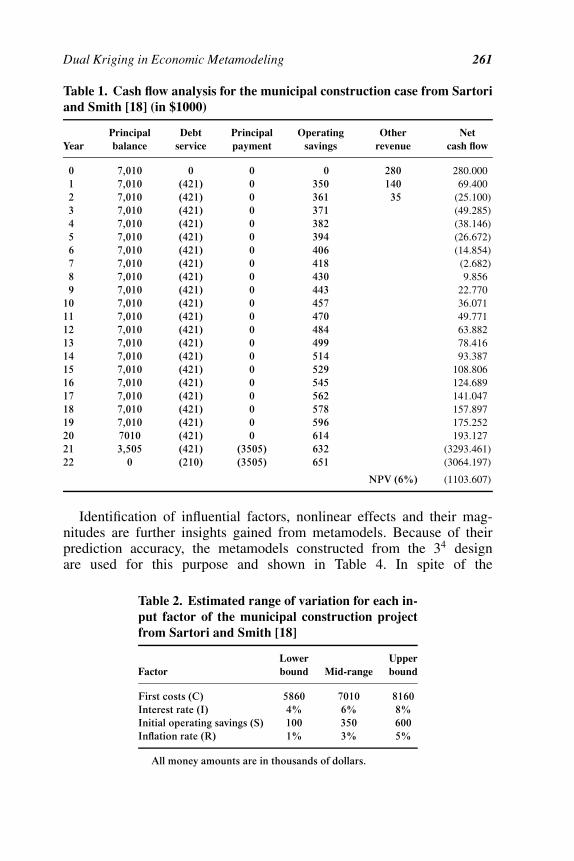
This case study was originally taken from Sartori and Smith [18]. It involvesthe proposed construction of a new municipal building in a north Pittsburghsuburb. The first cost of this investment is estimated to be $7,010 K. Thisinvestment is financed by a loan with an interest rate of 6%. The investmentis expected to generate annual savings of $350 K. The inflation rate isestimated to be 3%. Table 1 shows the cash flow analysis of this investmentunder the most likely condition.

Sartori and Smith identified four uncertain factors in this cash flow anal-ysis: first cost (C), interest rate (I), initial operating saving (S), and inflationrate (R). The reasonable ranges of these variables are shown in Table 2. Twoexperimental designs are studied: a three-level fractional factorial 34−1 witha mid range value design and a three-level full factorial 34 design. Thesedesigns generate 28 and 81 design points, respectively. A validation setof 40 observations and a generalization set of 200 observations are alsogenerated. The kriging model for the 34−1 data set uses a linear covariancefunction and distance of influence = 1. The ANN is best at 2 hidden neu-rons (after considering 1, 2, or 3) trained for 479 K iterations. The krigingmodel for the 34 data set uses a linear covariance function and distance ofinfluence = 0.5. The ANN is best at 5 hidden neurons (after considering 1through 6) trained for 4,913 K iterations.

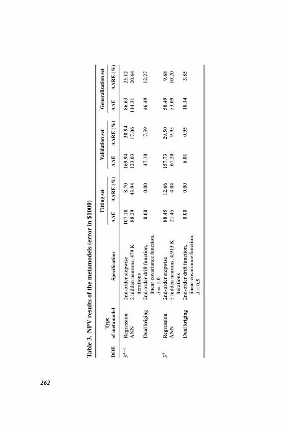
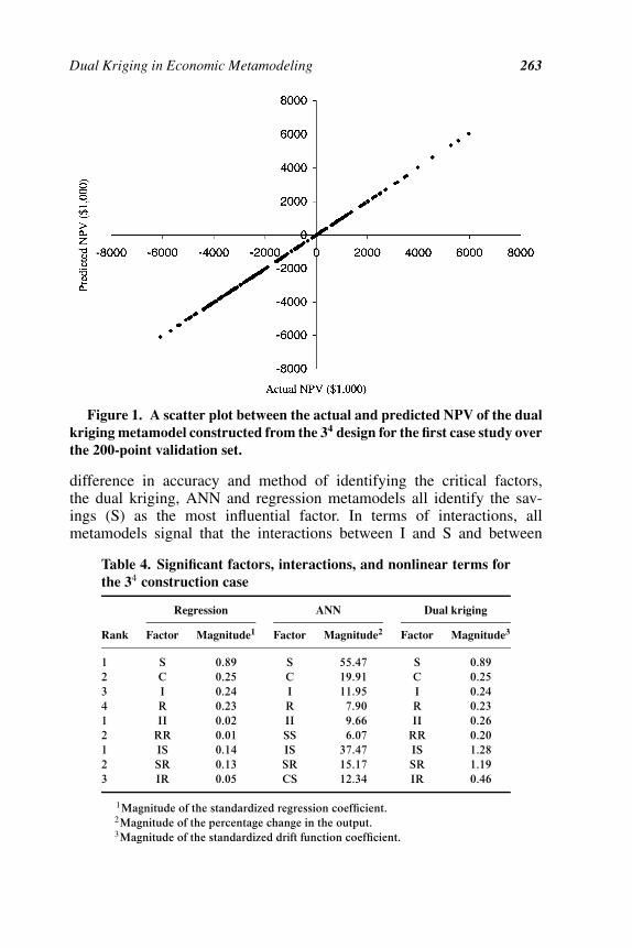
Table 3 shows the error in prediction of NPV of the metamodels. Sincedual kriging is an exact interpolation technique, the metamodel exactly fitsall data points in the fitting data set, thus leading to the absence of fittingerrors. Dual kriging considerably outperforms the polynomial regressionand the ANN metamodel in terms of prediction accuracy across all designsand data sets. Figure 1 shows the dual kriging predictions versus actuals forthe 200 point validation set and it is seen that the predictions are uniformlygood with no bias exhibited.


Table 1. Cash flow analysis for the municipal construction case from Sartoriand Smith [18] (in $1000)

YearPrincipalbalance

Debtservice

Principalpayment

Operatingsavings

Otherrevenue

Netcash flow

0 7,010 0 0 0 280 280.0001 7,010 (421) 0 350 140 69.4002 7,010 (421) 0 361 35 (25.100)3 7,010 (421) 0 371 (49.285)4 7,010 (421) 0 382 (38.146)5 7,010 (421) 0 394 (26.672)6 7,010 (421) 0 406 (14.854)7 7,010 (421) 0 418 (2.682)8 7,010 (421) 0 430 9.8569 7,010 (421) 0 443 22.770

10 7,010 (421) 0 457 36.07111 7,010 (421) 0 470 49.77112 7,010 (421) 0 484 63.88213 7,010 (421) 0 499 78.41614 7,010 (421) 0 514 93.38715 7,010 (421) 0 529 108.80616 7,010 (421) 0 545 124.68917 7,010 (421) 0 562 141.04718 7,010 (421) 0 578 157.89719 7,010 (421) 0 596 175.25220 7010 (421) 0 614 193.12721 3,505 (421) (3505) 632 (3293.461)22 0 (210) (3505) 651 (3064.197)

NPV (6%) (1103.607)

Identification of influential factors, nonlinear effects and their mag-nitudes are further insights gained from metamodels. Because of theirprediction accuracy, the metamodels constructed from the 34 designare used for this purpose and shown in Table 4. In spite of the

Table 2. Estimated range of variation for each in-put factor of the municipal construction projectfrom Sartori and Smith [18]

FactorLowerbound Mid-range

Upperbound

First costs (C) 5860 7010 8160Interest rate (I) 4% 6% 8%Initial operating savings (S) 100 350 600Inflation rate (R) 1% 3% 5%

All money amounts are in thousands of dollars.

Tabl

e3.

NP

Vre

sult

sof

the

met

amod

els

(err

orin

$100

0)

Fit

ting

set

Val

idat

ion

set

Gen

eral

izat

ion

set

DO

ET

ype

ofm

etam

odel

Spec

ifica

tion

AA

EA

AR

E(%

)A

AE

AA

RE

(%)

AA

EA

AR

E(%

)

34−1

Reg

ress

ion

2nd-

orde

rst

epw

ise

107.

188.

7016

9.94

30.9

486

.63

25.1

2A

NN

2hi

dden

neur

ons,

479

Kit

erat

ions

88.2

943

.94

123.

0317

.06

114.

3120

.64

Dua

lkri

ging

2nd-

orde

rdr

ift

func

tion

,lin

ear

cova

rian

cefu

ncti

on,

d=

1.0

0.00

0.00

47.1

07.

3946

.49

12.2

7

34R

egre

ssio

n2n

d-or

der

step

wis

e88

.45

12.6

615

7.73

29.5

050

.49

9.68

AN

N5

hidd

enne

uron

s,4,

913

Kit

erat

ions

21.4

54.

0467

.20

9.95

53.0

910

.20

Dua

lkri

ging

2nd-

orde

rdr

ift

func

tion

,lin

ear

cova

rian

cefu

ncti

on,

d=

0.5

0.00

0.00

6.01

0.95

18.1

43.

85

262


Figure 1. A scatter plot between the actual and predicted NPV of the dualkriging metamodel constructed from the 34 design for the first case study overthe 200-point validation set.

difference in accuracy and method of identifying the critical factors,the dual kriging, ANN and regression metamodels all identify the sav-ings (S) as the most influential factor. In terms of interactions, allmetamodels signal that the interactions between I and S and between

Table 4. Significant factors, interactions, and nonlinear terms forthe 34 construction case

Regression ANN Dual kriging

Rank Factor Magnitude1 Factor Magnitude2 Factor Magnitude3

1234

SCIR

0.890.250.240.23

SCIR

55.4719.9111.957.90

SCIR

0.890.250.240.23

12

IIRR

0.020.01

IISS

9.666.07

IIRR

0.260.20

123

ISSRIR

0.140.130.05

ISSRCS

37.4715.1712.34

ISSRIR

1.281.190.46

1Magnitude of the standardized regression coefficient.2Magnitude of the percentage change in the output.3Magnitude of the standardized drift function coefficient.


Table 5. Comparison of the estimated coststructure of the CMT and the FMS systemsfrom Park [14]

CMT FMS

Number of pieces produce/year 544,000 544,000Variable labor cost/part $2.15 $1.30Variable material cost/part $1.53 $1.10Annual overhead $3.15M $1.95MAnnual tooling costs $470,000 $300,000Annual inventory costs $141,000 $31,500Investments $3.5M $10MSalvage value $0.5M $1MService life 10 years 10 yearsDepreciation method (MACRS) 7-year 7-year

S and R are the most important. The quadratic effect of I is alsoimportant.

An FMS Case Study

An FMS case was selected and modified from Park [14]. A U.S. companywill determine whether to replace a conventional manufacturing technol-ogy (CMT) with a flexible manufacturing system (FMS). Table 5 showsthe comparison of the estimated cost structure of both systems. The firm’smarginal tax rate and MARR are projected to be 40% and 15%, respec-tively. The incremental cash flow analysis for CMT and FMS is shown inTable 6.

Park stated that the management of this company was very confidentabout all estimates for CMT. However, the firm did not have any previ-ous experience in operating an FMS. Ten uncertain factors for the FMSare identified: variable labor cost per part (L), variable material cost perpart (M), annual overhead (O), annual tooling costs (T), annual inventorycosts (V), first investment (I), salvage value (S), tax rate (X), discountrate (D), and service life (L). Table 7 depicts a reasonable range for eachfactor. An experimental design of a three-level fractional factorial 310−5

with a mid range value design is used and generates 257 design points.The validation data set has 120 data points and the generalization data setconsists of 200 data points. Because ANN are sensitive to number of inputvariables, an ANN metamodel with all input variables is used to identifythe critical factors, their quadratic effects, and their interactions. Then,

Tabl

e6.

An

incr

emen

talc

ash

flow

anal

ysis

for

CM

Tan

dF

MS

from

Par

k[1

4](i

n$1

000)

Yea

r0

12

34

56

78

910

Inco

me

stat

emen

tR

even

ueL

abor

462.

4046

2.40

462.

4046

2.40

462.

4046

2.40

462.

4046

2.40

462.

4046

2.40

Mat

eria

l23

3.92

233.

9223

3.92

233.

9223

3.92

233.

9223

3.92

233.

9223

3.92

233.

92O

verh

ead

1200

.00

1200

.00

1200

.00

1200

.00

1200

.00

1200

.00

1200

.00

1200

.00

1200

.00

1200

.00

Too

ling

170.

0017

0.00

170.

0017

0.00

170.

0017

0.00

170.

0017

0.00

170.

0017

0.00

Inve

ntor

y10

9.50

109.

5010

9.50

109.

5010

9.50

109.

5010

9.50

109.

5010

9.50

109.

50D

epre

ciat

ion

928.

8515

91.8

511

36.8

581

1.85

580.

4557

9.80

580.

4528

9.90

Tax

able

inco

me

1246

.97

583.

9710

38.9

713

63.9

715

95.3

715

96.0

215

95.3

718

85.9

221

75.8

221

75.8

2In

com

eta

x(4

0%)

498.

7923

3.59

415.

5954

5.59

638.

1563

8.41

638.

1575

4.37

870.

3387

0.33

Net

inco

me

748.

1835

0.38

623.

3881

8.38

957.

2295

7.61

957.

2211

31.5

513

05.4

913

05.4

9C

ash

flow

stat

emen

tC

ash

from

oper

atio

nN

etin

com

e74

8.18

350.

3862

3.38

818.

3895

7.22

957.

6195

7.22

1131

.55

1305

.49

1305

.49

Dep

reci

atio

n92

8.85

1591

.85

1136

.85

811.

8558

0.45

579.

8058

0.45

289.

90In

vest

men

t&

salv

age

(650

0)50

0.00

Gai

nta

x(4

0%)

(200

.00)

Net

cash

flow

(650

0)16

77.0

319

42.2

317

60.2

316

30.2

315

37.6

715

37.4

115

37.6

714

21.4

513

05.4

916

05.4

9N

PV

(15%

)17

56.2

25

265


Table 7. Uncertain factors and their ranges for the FMS casefrom Park [14]

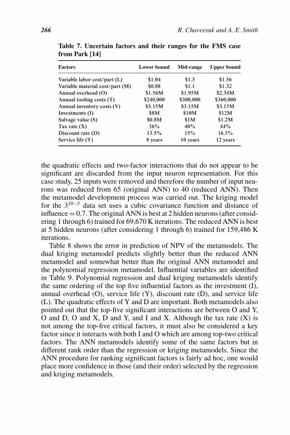
Factors Lower bound Mid-range Upper bound

Variable labor cost/part (L) $1.04 $1.3 $1.56Variable material cost/part (M) $0.88 $1.1 $1.32Annual overhead (O) $1.56M $1.95M $2.34MAnnual tooling costs (T) $240,000 $300,000 $360,000Annual inventory costs (V) $3.15M $3.15M $3.15MInvestments (I) $8M $10M $12MSalvage value (S) $0.8M $1M $1.2MTax rate (X) 36% 40% 44%Discount rate (D) 13.5% 15% 16.5%Service life (Y) 8 years 10 years 12 years

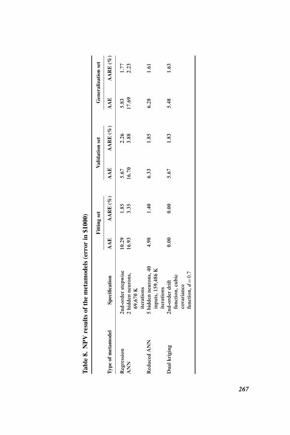
the quadratic effects and two-factor interactions that do not appear to besignificant are discarded from the input neuron representation. For thiscase study, 25 inputs were removed and therefore the number of input neu-rons was reduced from 65 (original ANN) to 40 (reduced ANN). Thenthe metamodel development process was carried out. The kriging modelfor the 310−5 data set uses a cubic covariance function and distance ofinfluence = 0.7. The original ANN is best at 2 hidden neurons (after consid-ering 1 through 6) trained for 69,670 K iterations. The reduced ANN is bestat 5 hidden neurons (after considering 1 through 6) trained for 159,486 Kiterations.

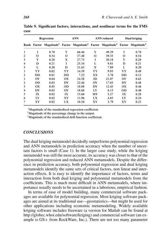
Table 8 shows the error in prediction of NPV of the metamodels. Thedual kriging metamodel predicts slightly better than the reduced ANNmetamodel and somewhat better than the original ANN metamodel andthe polynomial regression metamodel. Influential variables are identifiedin Table 9. Polynomial regression and dual kriging metamodels identifythe same ordering of the top five influential factors as the investment (I),annual overhead (O), service life (Y), discount rate (D), and service life(L). The quadratic effects of Y and D are important. Both metamodels alsopointed out that the top-five significant interactions are between O and Y,O and D, O and X, D and Y, and I and X. Although the tax rate (X) isnot among the top-five critical factors, it must also be considered a keyfactor since it interacts with both I and O which are among top-two criticalfactors. The ANN metamodels identify some of the same factors but indifferent rank order than the regression or kriging metamodels. Since theANN procedure for ranking significant factors is fairly ad hoc, one wouldplace more confidence in those (and their order) selected by the regressionand kriging metamodels.

Tabl

e8.

NP

Vre

sult

sof

the

met

amod

els

(err

orin

$100

0)

Fit

ting

set

Val

idat

ion

set

Gen

eral

izat

ion

set

Typ

eof

met

amod

elSp

ecifi

cati

onA

AE

AA

RE

(%)

AA

EA

AR

E(%

)A

AE

AA

RE

(%)

Reg

ress

ion

2nd-

orde

rst

epw

ise

10.2

91.

855.

672.

265.

831.

77A

NN

2hi

dden

neur

ons,

69,6

70K

iter

atio

ns

16.9

33.

3516

.70

3.88

17.6

92.

23

Red

uced

AN

N5

hidd

enne

uron

s,40

inpu

ts,1

59,4

86K

iter

atio

ns

4.98

1.40

6.33

1.85

6.28

1.61

Dua

lkri

ging

2nd-

orde

rdr

ift

func

tion

,cub

icco

vari

ance

func

tion

,d=

0.7

0.00

0.00

5.67

1.83

5.48

1.63

267


Table 9. Significant factors, interactions, and nonlinear terms for the FMScase

Regression ANN ANN reduced Dual kriging

Rank Factor Magnitude1 Factor Magnitude2 Factor Magnitude2 Factor Magnitude3

12345

IOYDL

0.700.540.280.210.20

YOXID

66.4637.4827.7525.3421.63

YOILX

49.2939.3530.18

9.817.89

IOYDL

0.700.540.280.210.20

12

YYDD

0.020.01

YYDD

14.597.22

YYXX

9.933.70

YYDD

0.490.12

1234567

OYODOXDYIXLYXY

0.040.030.030.030.020.020.02

OXDYODOYIXXYLX

24.5822.4618.8818.6815.6011.9610.20

IDOYDYLYMYLXXY

21.0717.8312.45

6.135.274.853.79

OYDYOXODIXLYXY

0.650.480.460.400.280.240.23

1Magnitude of the standardized regression coefficient.2Magnitude of the percentage change in the output.3Magnitude of the standardized drift function coefficient.

CONCLUSIONS

The dual kriging metamodel decidedly outperforms polynomial regressionand ANN metamodels in prediction accuracy when the number of uncer-tain factors is small (Case 1). In the larger case study, while the krigingmetamodel was still the most accurate, its accuracy was closer to that of thepolynomial regression and reduced ANN metamodels. Despite the differ-ence in prediction accuracy, both polynomial regression and dual krigingmetamodels identify the same sets of critical factors, non linear and inter-action effects. It is easy to identify the importance of factors, terms andinteraction from both dual kriging and polynomial metamodels from thecoefficients. This is much more difficult in ANN metamodels, where im-portance usually needs to be ascertained in a laborious, empirical fashion.

In terms of ease of model building, many commercial software pack-ages are available for polynomial regression. Most kriging software pack-ages are aimed at its traditional use—geostatistics—but might be used forother applications including economic metamodeling. Widely availablekriging software includes freeware (a version for Matlab can be found athttp://globec.whoi.edu/software/kriging) and commercial software (an ex-ample is GS+ from RockWare, Inc.). There are not too many parameter


choices for dual kriging and the method is computationally similar to a leastsquares regression method in terms of procedure and computational effort.ANN has widely available commercial software but the model building andvalidation are much more artful and laborious than in regression or krigingand require greater experiential knowledge in the field.

Since kriging leverages the spatial relationship among data, it may findparticularly good application in engineering economics problems whereobservations are limited but there is definite (or assumed) correlation amongthe input data. Besides the metamodeling application herein, one couldforesee the use of kriging for cost estimation.

REFERENCES

[1] Barton, R.R., “Metamodels for simulation input-output relations,” in Proceedingsof the 1992 Winter Simulation Conference, 1992, pp. 289–299.

[2] Booker, A.J., “Design and analysis of computer experiments,” 7th AIAA/USAF/NASA/ISSMO Symposium on Multidisciplinary Analysis & Optimization,St. Louis, MO, AIAA, 1998, pp. 118–128.

[3] Chaveesuk, R. and A.E. Smith, “Economic valuation of capital projects usingneural network metamodels,”The Engineering Economist, Vol. 48, No. 1, 2003,pp. 1–30.

[4] Cressie, N.A.C., Statistics for Spatial Data, NY: John Wiley & Son, 1991.[5] Deloreme, S., Y. Petit, J.A. De Guise, C.-E. Aubin, H. Labelle, C. Landry and

J. Dansereau, “Three-dimensional modelling and rendering of the human skeletaltrunk from 2D radiographic images,” Proceedings of the Second InternationalConference on 3-D Imaging and Modeling, Ottawa, Ontario, Canada, OctoberVol. 4–8, 1999, pp. 497–505.

[6] Echaabi, J., F. Trochu, and R. Gauvin, “A general strength theory for compositematerials based on dual kriging interpolation,” Journal of Reinforced Plastics andComposites, Vol. 14, 1995, pp. 211–232.

[7] Echaabi, J., F. Trochu, and R. Gauvin, “Review of failure criteria for fibrouscomposite materials,” Polimer Composites, Vol. 17, No. 6, 1996, pp. 786–798.

[8] Echaabi, J. and F. Trochu, “A methodology to derive the implicit equation offailure criteria for fibrous composite laminates,” Journal of Composite Materials,Vol. 30, No. 10, 1996, pp. 1088–1114.

[9] Eschenbach, T.G. and L.S. McKeague, “Exposition on using graphs for sensi-tivity analysis,” The Engineering Economist, Vol. 34, No. 4, 1989, pp. 315–333.

[10] Journel, A.G. and Ch. J. Huijbregts, Mining Geostatistics, NY: Academic Press,1978.

[11] Kleijnen, J.P.C., “Regression metamodels for generalizing simulation results,”IEEE Transactions on Systems, Man, and Cybernetics, Vol. SMC-9, 1979, pp. 93–96.

[12] Kleijnen, J.P.C. and R.G. Sargent, “A methodology for fitting and validatingmetamodels in simulation,” European Journal of Operational Research, Vol. 120,2000, pp. 14–29.


[13] Mamat, A., F. Trochu, and B. Sanschagrin, “Analysis of shrinkage by dual krigingfor filled and unfilled polypropylene molded parts,” Polymer Engineering andScience, Vol. 35, No. 19, 1995, pp. 1511–1520.

[14] Park, C., Contemporary Engineering Economic Case Studies, Reading, MA:Addison-Wesley, 1993.

[15] Porier, C. and R. Tinawi, “Finite element stress tensor fields interpolation andmanipulation using 3D dual kriging,” Computers & Structures, Vol. 40, No. 2,1991, pp. 211–222.

[16] Ratle, A., “Accelerating the Convergence of Evolutionary Algorithms by FitnessLandscape Approximation,” in Proceedings of the 5th International Conferenceon Parallel Problem Solving from Nature-PPSN V, Amsterdam, The Netherlands,September 1998, pp. 87–96.

[17] Sacks, J., W.H. Welch, T.J. Mitchell, and H.P. Wynn, “Design and analysis ofcomputer experiments,” Statistical Science, Vol. 4, 1989, pp. 409–435.

[18] Sartori, D.E. and A.E. Smith, “A metamodel approach to sensitivity analysis ofcapital project valuation,” The Engineering Economist, Vol. 43, 1997, pp. 1–24.

[19] Simpson, T.W., T.M. Mauery, J.J. Korte, and F. Mistree, “Comparison of re-sponse surface and kriging models for multidisciplinary design optimization,”7th AIAA/USAF/NASA/ISSMO Symposium on Multidisciplinary Analysis & Opti-mization, St. Louis, MO, AIAA, September 2–4, 1998, pp. 381–391.

[20] Terriault, P., M.-A. Meunier, and F. Trochu, “Application of dual kriging tothe construction of a general phenomenological material law for shape mem-ory alloys,” Journal of Intelligent Material Systems and Structures, Vol. 8, 1998,pp. 605–618.

[21] Trochu, F., “A contouring program based on dual kriging interpolation,” Engi-neering with Computers, 1993, pp. 160–177.

[22] Trochu, F. and P. Terriault, “Nonlinear modeling of hysteretic material lawsby dual kriging and application,” Computer Methods in Applied Mechanics andEngineering, Vol. 151, 1998, pp. 545–558.

[23] Trochu, F., N. Sacepe, O. Volkov, and S. Turenne, “Characterization of NiTishape memory alloys using dual kriging interpolation,” Materials Science andEngineering, Vol. A273–275, 1999, pp. 395–399.

[24] Van Groenendaal, W.J.H., “Estimating NPV variability for deterministic mod-els,” European Journal of Operational Research, Vol. 107, 1998, pp. 202–213.

[25] Van Groenendaal, W.J.H. and J.P.C. Kleijnen, “Identifying important factors indeterministic investment problems using design of experiment,” in Proceedingsof the 1998 Winter Simulation Conference, December 13–16, 1998, pp. 713–718.

BIOGRAPHICAL SKETCH

RAVIPIM CHAVEESUK is an Assistant Professor in the Department of Management of Agro-Industrial Technology (an interdisciplinary graduate program) at Kasetsart University,Bangkok, Thailand. She received a B.S. in Agro-Industrial Product Development fromKasetsart University, Thailand, a M.S. in Food Science and Agricultural Chemistry fromMcGill University in Canada, and a M.S. and Ph.D. in Industrial Engineering from Uni-versity of Pittsburgh. While at the University of Pittsburgh she was a Royal Thai Scholar.


Dr. Chaveesuk also had a post doctoral position in industrial engineering at Auburn Uni-versity. Her primary research interest is in the area of engineering economics.

ALICE E. SMITH is Professor and Chair of the Industrial and Systems Engineering Departmentat Auburn University. Previous to this position, she was on the faculty of the Departmentof Industrial Engineering at the University of Pittsburgh, which she joined in 1991 after tenyears of industrial experience with Southwestern Bell Corporation. Dr. Smith has degreesin engineering and business from Rice University, Saint Louis University and Universityof Missouri—Rolla. Her research in analysis, modeling and optimization of manufactur-ing processes and engineering design has been funded by NASA, the National Institute ofStandards (NIST), Lockheed Martin, Adtranz (now Bombardier Transportation), the BenFranklin Technology Center of Western Pennsylvania and the National Science Foundation(NSF), from which she was awarded a CAREER grant in 1995 and an ADVANCE Lead-ership grant in 2001. Dr. Smith has served as a principal investigator on over $3 million ofsponsored research. Dr. Smith holds one U.S. patent and several international patents andhas authored over 50 publications in books and journals including articles in IIE Transac-tions, IEEE Transactions on Reliability, INFORMS Journal on Computing, InternationalJournal of Production Research, IEEE Transactions on Systems, Man, and Cybernetics,Journal of Manufacturing Systems, The Engineering Economist, and IEEE Transactions onEvolutionary Computation. Dr. Smith holds editorial positions on INFORMS Journal onComputing, Computers & Operations Research, International Journal of General Systems,IEEE Transactions on Evolutionary Computation and IIE Transactions. Dr. Smith is a fel-low of IIE, a senior member of IEEE and SWE, a member of Tau Beta Pi, INFORMS andASEE, and a Registered Professional Engineer in Industrial Engineering in Alabama andPennsylvania.

DUAL KRIGING: AN EXPLORATORY USE IN … Kriging...Dual Kriging in Economic Metamodeling 249...

Documents

Transcript of DUAL KRIGING: AN EXPLORATORY USE IN … Kriging...Dual Kriging in Economic Metamodeling 249...