Dual Giant Gravitons&

Emergent CurvatureMichael Gary

arXiv:1011.5231 w/ R. Eager & M. M. Roberts

Wednesday, January 18, 2012

Motivation

Understand emergent geometry in AdS/CFT.

Anomalies are protected, so CFT calculations can be trusted.

Explore and corrections.

New predictions/tests for AdS/CFT.

1/N2 α�

Wednesday, January 18, 2012

OutlineReview of AdS/CFT & the Geometric Setup

The Hilbert Series

Dual Giant Gravitons

The Hilbert Series Revisited

Curvature from Counting

Conclusions & Future Directions

Wednesday, January 18, 2012

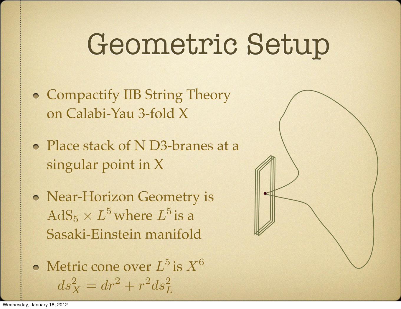
Compactify IIB String Theory on Calabi-Yau 3-fold X

Place stack of N D3-branes at a singular point in X

Near-Horizon Geometry is where is a Sasaki-Einstein manifold

Metric cone over is

Geometric Setup

AdS5 × L5 L5

L5 X6

ds2X = dr2 + r2ds2L

Wednesday, January 18, 2012

Dual Description

The dual description is an =1 SCFT, the low energy theory on the stack of D3-branes.

The =1 SCFT has a global U(1) R-Symmetry.

The U(1) R-symmetry is dual to the U(1) generated by the Reeb vector .

N

N

ξ = J(r∂r)

Wednesday, January 18, 2012

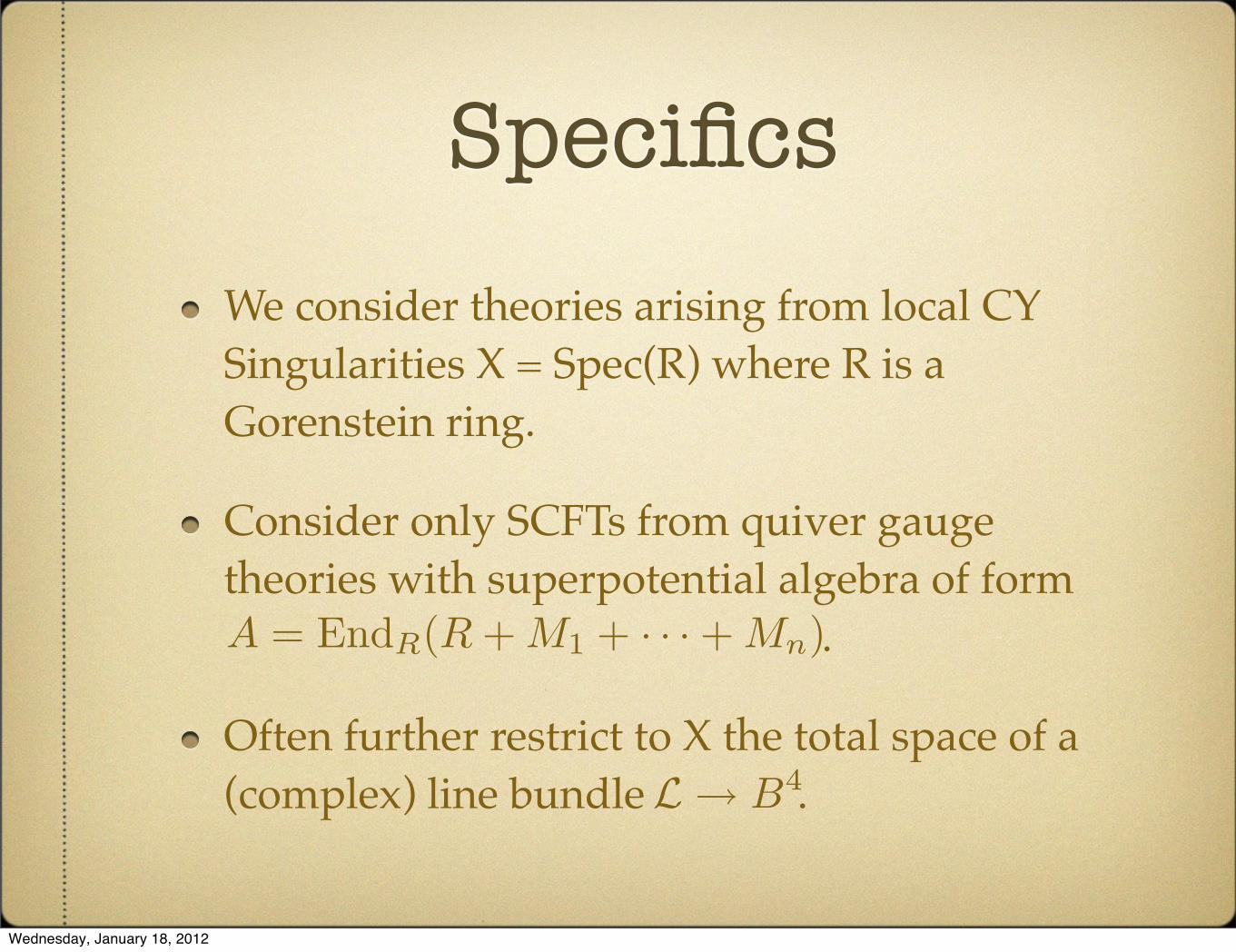
SpecificsWe consider theories arising from local CY Singularities X = Spec(R) where R is a Gorenstein ring.

Consider only SCFTs from quiver gauge theories with superpotential algebra of form .

Often further restrict to X the total space of a (complex) line bundle . L→ B4

A = EndR(R + M1 + · · · + Mn)

Wednesday, January 18, 2012

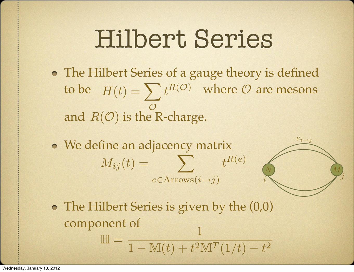
Hilbert SeriesThe Hilbert Series of a gauge theory is defined to be where are mesons

and is the R-charge.

We define an adjacency matrix

The Hilbert Series is given by the (0,0) component of

H(t) =�

O

tR(O) O

R(O)

Mij(t) =�

e∈Arrows(i→j)

tR(e)

H =1

1−M(t) + t2MT (1/t)− t2

N Mi j

ei→j

Wednesday, January 18, 2012

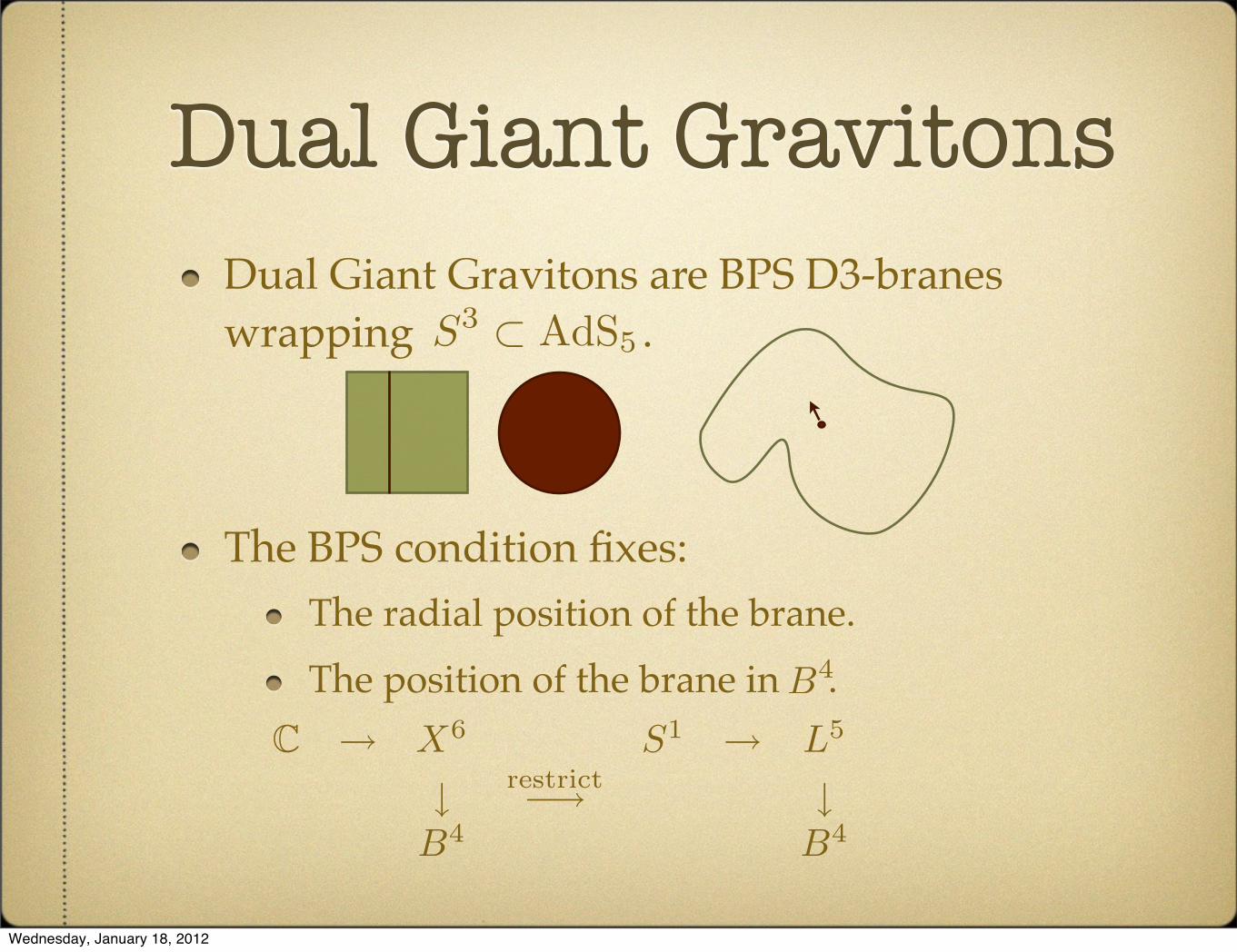
Dual Giant GravitonsDual Giant Gravitons are BPS D3-branes wrapping .

The BPS condition fixes:The radial position of the brane.The position of the brane in .

S3 ⊂ AdS5

B4

C → X6 S1 → L5

↓ restrict−→ ↓B4 B4

Wednesday, January 18, 2012

Dual Giant Gravitons

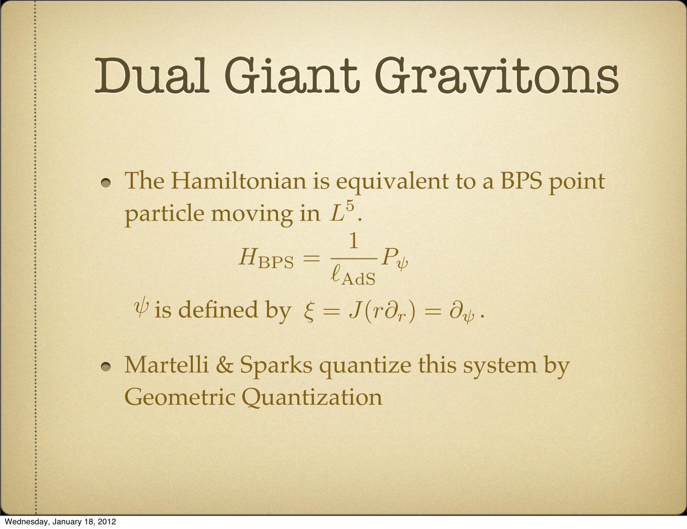
The Hamiltonian is equivalent to a BPS point particle moving in .

is defined by .

Martelli & Sparks quantize this system by Geometric Quantization

HBPS =1

�AdSPψ

L5

ξ = J(r∂r) = ∂ψψ

Wednesday, January 18, 2012

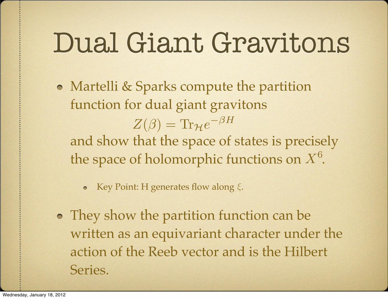
Dual Giant GravitonsMartelli & Sparks compute the partition function for dual giant gravitons

and show that the space of states is precisely the space of holomorphic functions on .

Key Point: H generates flow along .

They show the partition function can be written as an equivariant character under the action of the Reeb vector and is the Hilbert Series.

Z(β) = TrHe−βH

X6

ξ

Wednesday, January 18, 2012

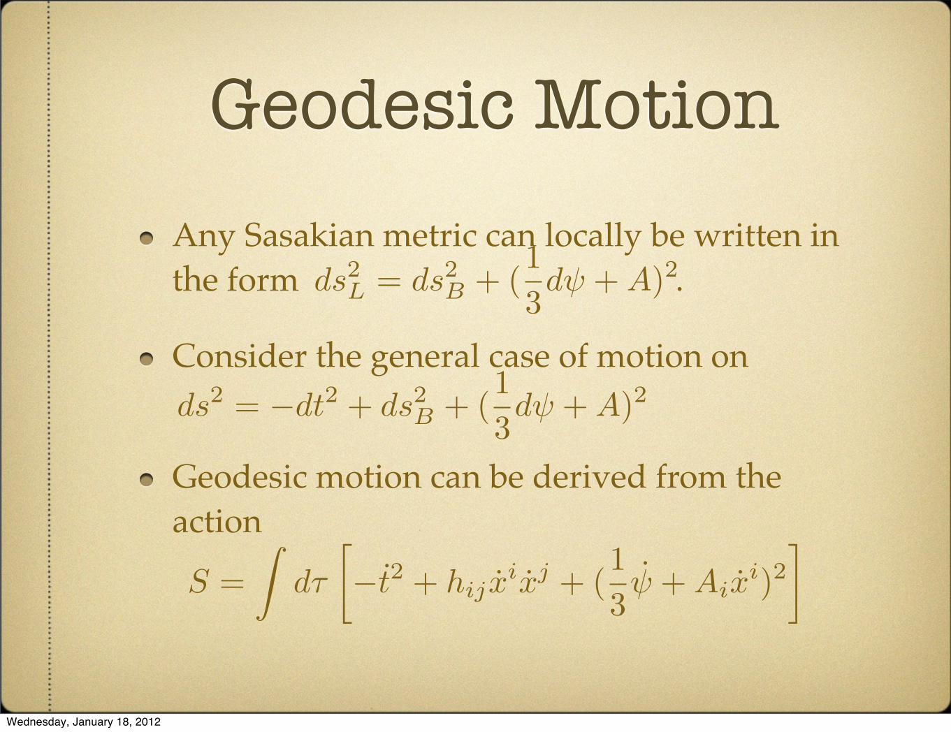
Geodesic MotionAny Sasakian metric can locally be written in the form .

Consider the general case of motion on

Geodesic motion can be derived from the action

ds2L = ds2B + (

13dψ + A)2

ds2 = −dt2 + ds2B + (13dψ + A)2

S =�

dτ

�−ṫ2 + hij ẋiẋj + (

13ψ̇ + Aiẋi)2

�

Wednesday, January 18, 2012

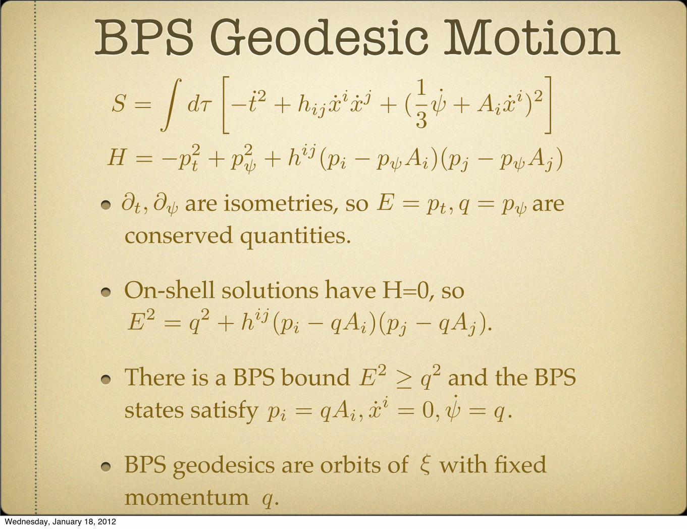
BPS Geodesic Motion

are isometries, so are conserved quantities.

On-shell solutions have H=0, so .

There is a BPS bound and the BPS states satisfy .

BPS geodesics are orbits of with fixed momentum .

S =�

dτ

�−ṫ2 + hij ẋiẋj + (

13ψ̇ + Aiẋi)2

�

H = −p2t + p2ψ + hij(pi − pψAi)(pj − pψAj)

∂t, ∂ψ E = pt, q = pψ

E2 = q2 + hij(pi − qAi)(pj − qAj)

E2 ≥ q2

pi = qAi, ẋi = 0, ψ̇ = q

ξ

qWednesday, January 18, 2012

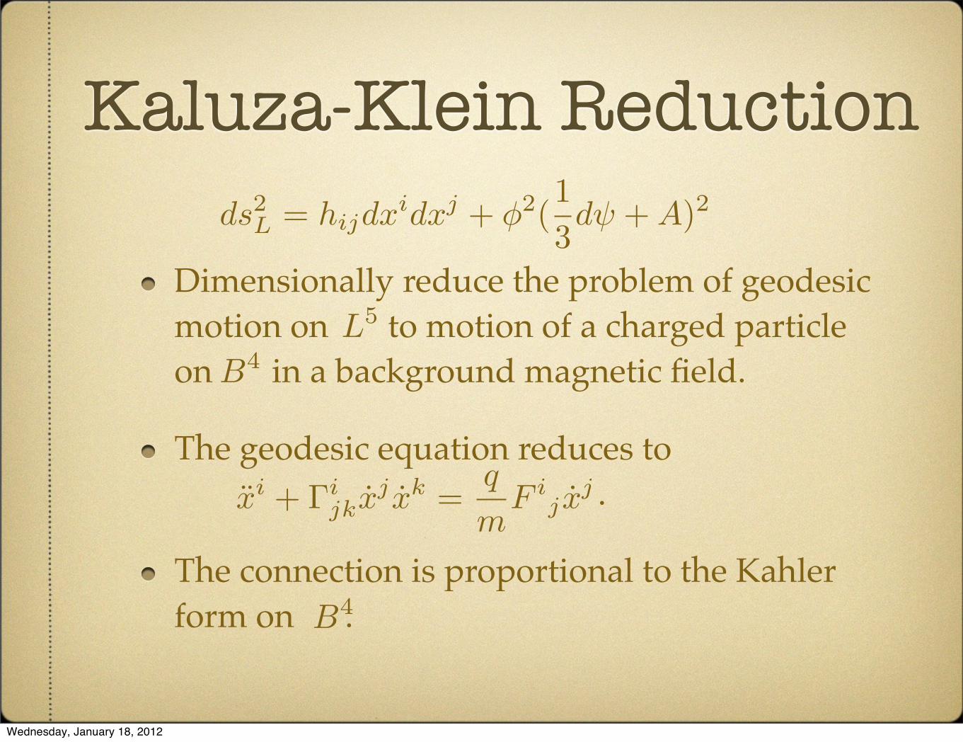
Kaluza-Klein Reduction

Dimensionally reduce the problem of geodesic motion on to motion of a charged particle on in a background magnetic field.

The geodesic equation reduces to .

The connection is proportional to the Kahler form on .

ds2L = hijdxidxj + φ2(

13dψ + A)2

L5

B4

ẍi + Γijkẋj ẋk =

q

mF ij ẋ

j

B4

Wednesday, January 18, 2012

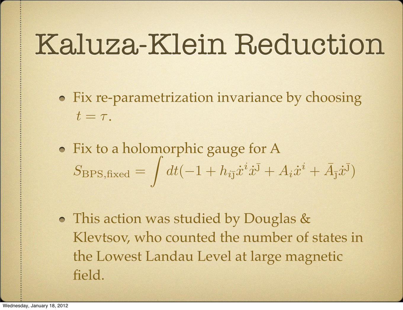
Kaluza-Klein ReductionFix re-parametrization invariance by choosing .

Fix to a holomorphic gauge for A

This action was studied by Douglas & Klevtsov, who counted the number of states in the Lowest Landau Level at large magnetic field.

t = τ

SBPS,fixed =�

dt(−1 + hīẋiẋ̄ + Aiẋi + Ā̄ẋ̄)

Wednesday, January 18, 2012

Hilbert Series Revisited

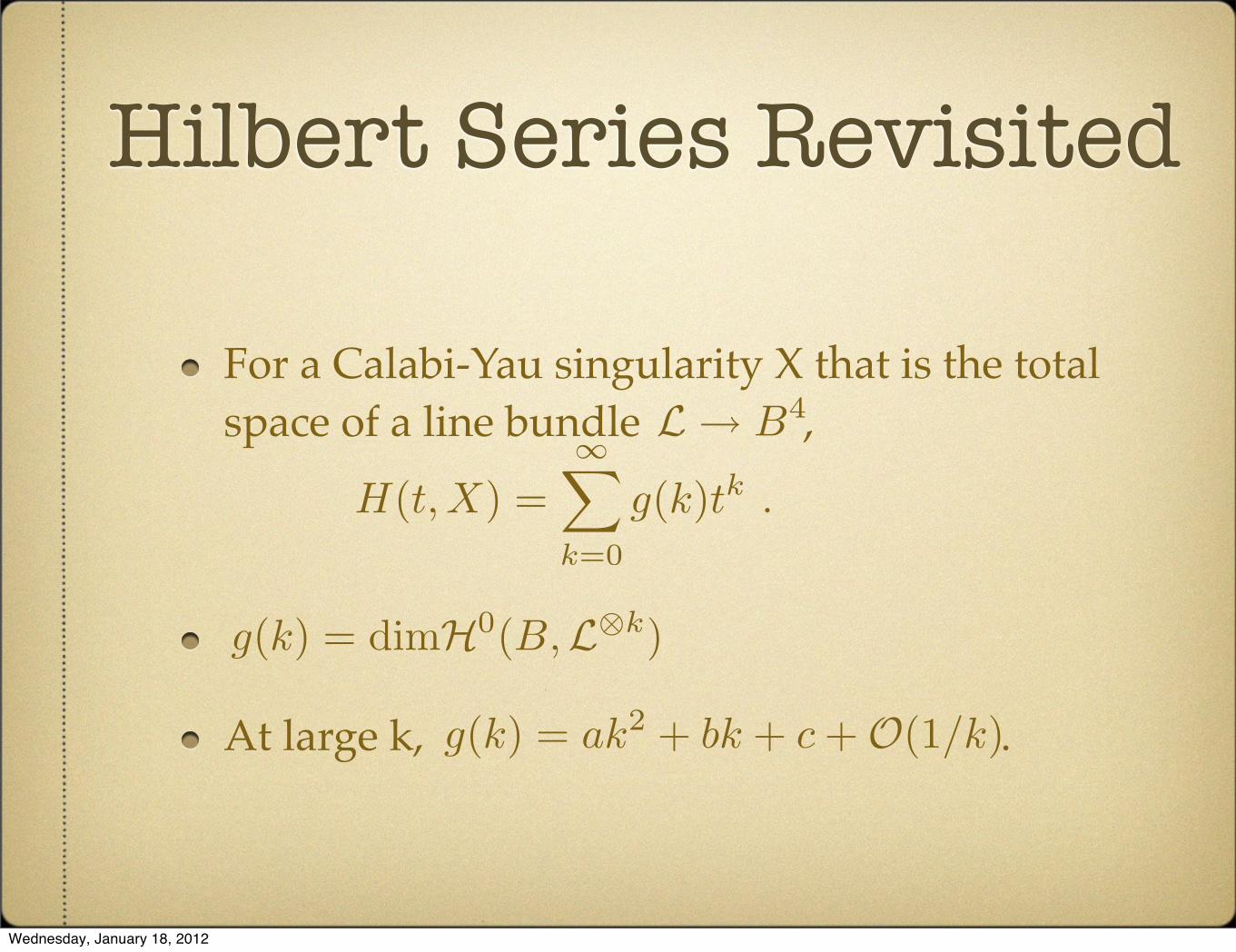
For a Calabi-Yau singularity X that is the total space of a line bundle ,

At large k, .

L→ B4

H(t, X) =∞�

k=0

g(k)tk .

g(k) = dimH0(B,L⊗k)

g(k) = ak2 + bk + c +O(1/k)

Wednesday, January 18, 2012

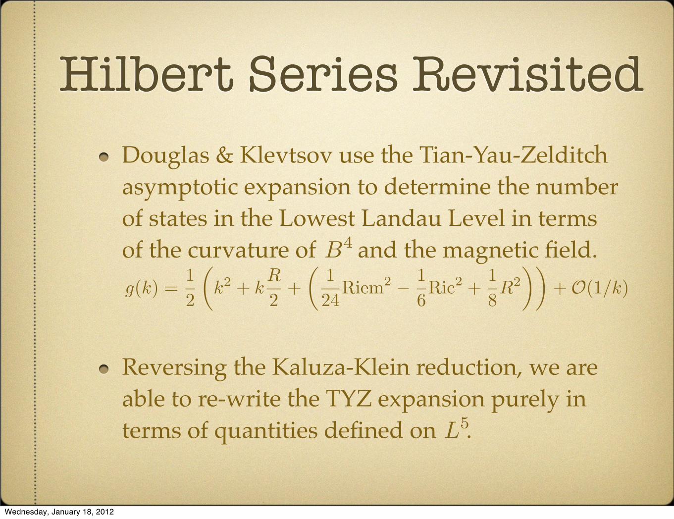
Hilbert Series RevisitedDouglas & Klevtsov use the Tian-Yau-Zelditch asymptotic expansion to determine the number of states in the Lowest Landau Level in terms of the curvature of and the magnetic field.

Reversing the Kaluza-Klein reduction, we are able to re-write the TYZ expansion purely in terms of quantities defined on .

B4

L5

g(k) =12

�k2 + k

R

2+

�124

Riem2 − 16Ric2 +

18R2

��+O(1/k)

Wednesday, January 18, 2012

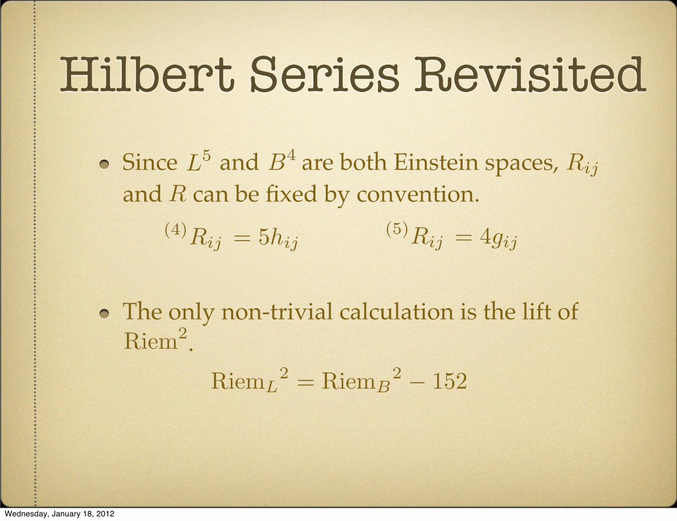
Hilbert Series RevisitedSince and are both Einstein spaces, and can be fixed by convention.

The only non-trivial calculation is the lift of .

L5 B4 RijR

Riem2

RiemL2 = RiemB2 − 152

(4)Rij = 5hij (5)Rij = 4gij

Wednesday, January 18, 2012

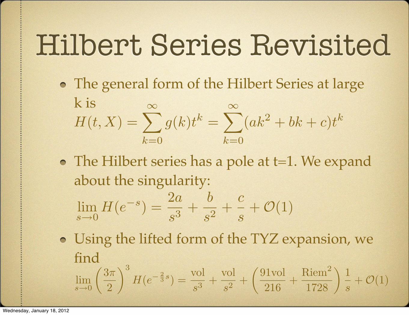
Hilbert Series RevisitedThe general form of the Hilbert Series at large k is

The Hilbert series has a pole at t=1. We expand about the singularity:

Using the lifted form of the TYZ expansion, we find

H(t, X) =∞�

k=0

g(k)tk =∞�

k=0

(ak2 + bk + c)tk

lims→0

H(e−s) =2as3

+b

s2+

c

s+O(1)

lims→0

�3π2

�3H(e−

23 s) =

vols3

+vols2

+�

91vol216

+Riem2

1728

�1s

+O(1)

Wednesday, January 18, 2012

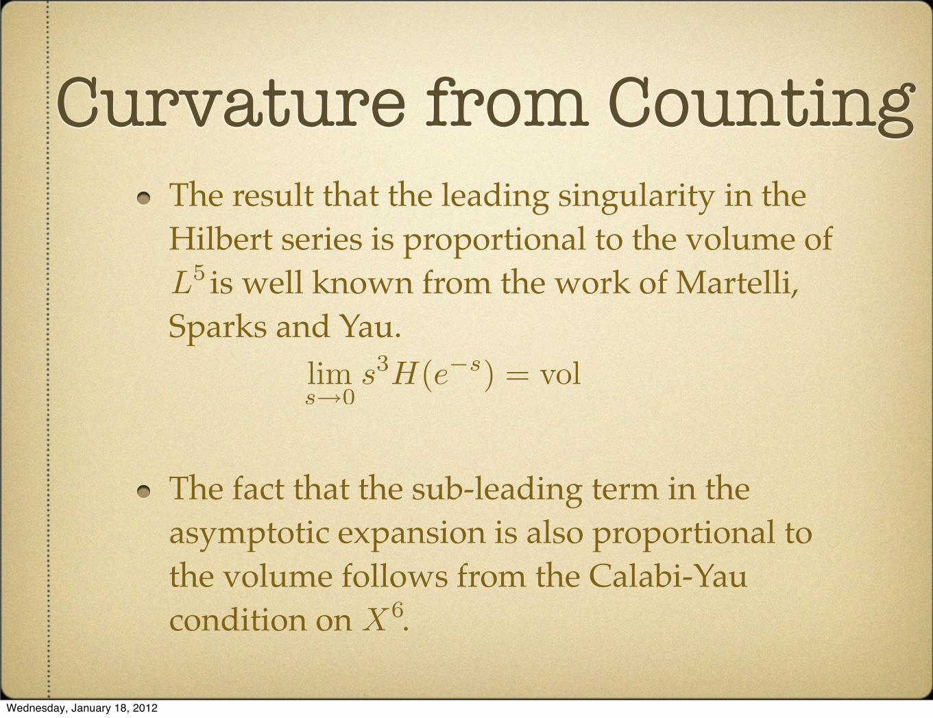
Curvature from CountingThe result that the leading singularity in the Hilbert series is proportional to the volume of is well known from the work of Martelli, Sparks and Yau.

The fact that the sub-leading term in the asymptotic expansion is also proportional to the volume follows from the Calabi-Yau condition on .

L5

X6

lims→0

s3H(e−s) = vol

Wednesday, January 18, 2012

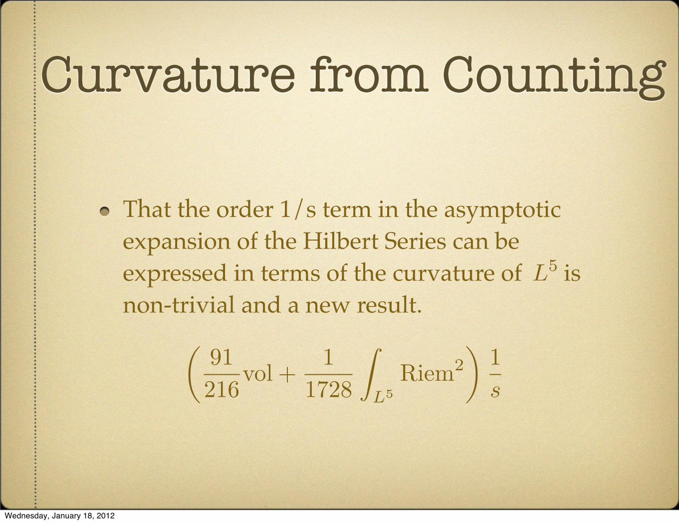
Curvature from Counting

That the order 1/s term in the asymptotic expansion of the Hilbert Series can be expressed in terms of the curvature of is non-trivial and a new result.

L5

�91216

vol +1

1728

�

L5Riem2

�1s

Wednesday, January 18, 2012

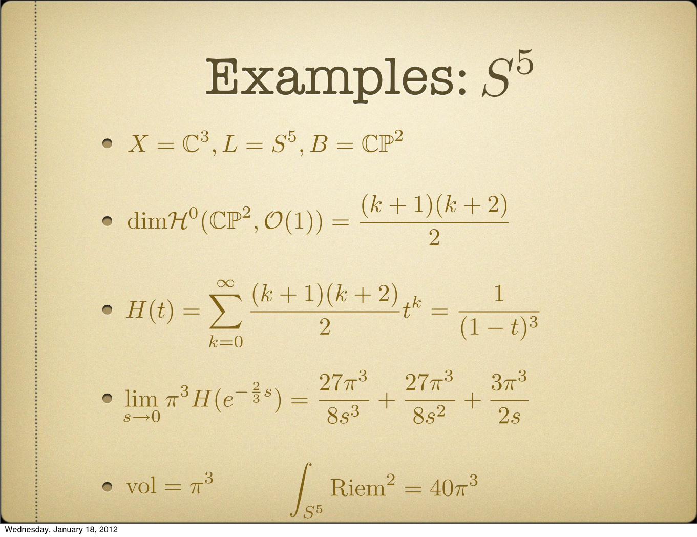
Examples:

S5

X = C3, L = S5, B = CP2

H(t) =∞�

k=0

(k + 1)(k + 2)2

tk =

1(1− t)3

dimH0(CP2,O(1)) = (k + 1)(k + 2)2

lims→0

π3H(e−23 s) =

27π3

8s3+

27π3

8s2+

3π3

2s

vol = π3�

S5Riem2 = 40π3

Wednesday, January 18, 2012

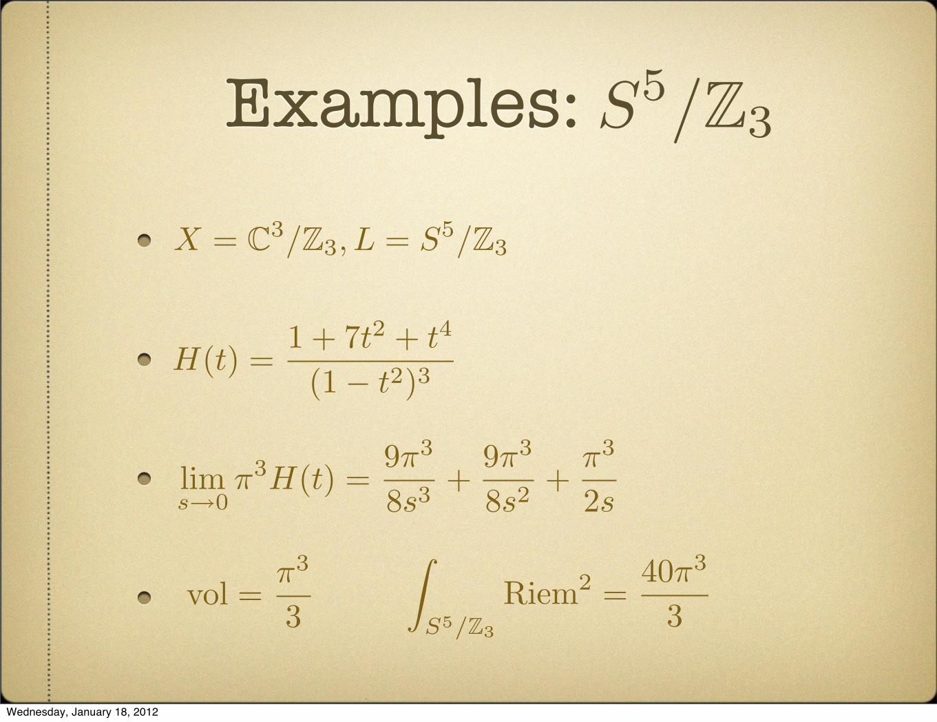
Examples:

X = C3/Z3, L = S5/Z3

H(t) =1 + 7t2 + t4

(1− t2)3

lims→0

π3H(t) =9π3

8s3+

9π3

8s2+

π3

2s

vol =π3

3

�

S5/Z3Riem2 =

40π3

3

S5/Z3

Wednesday, January 18, 2012

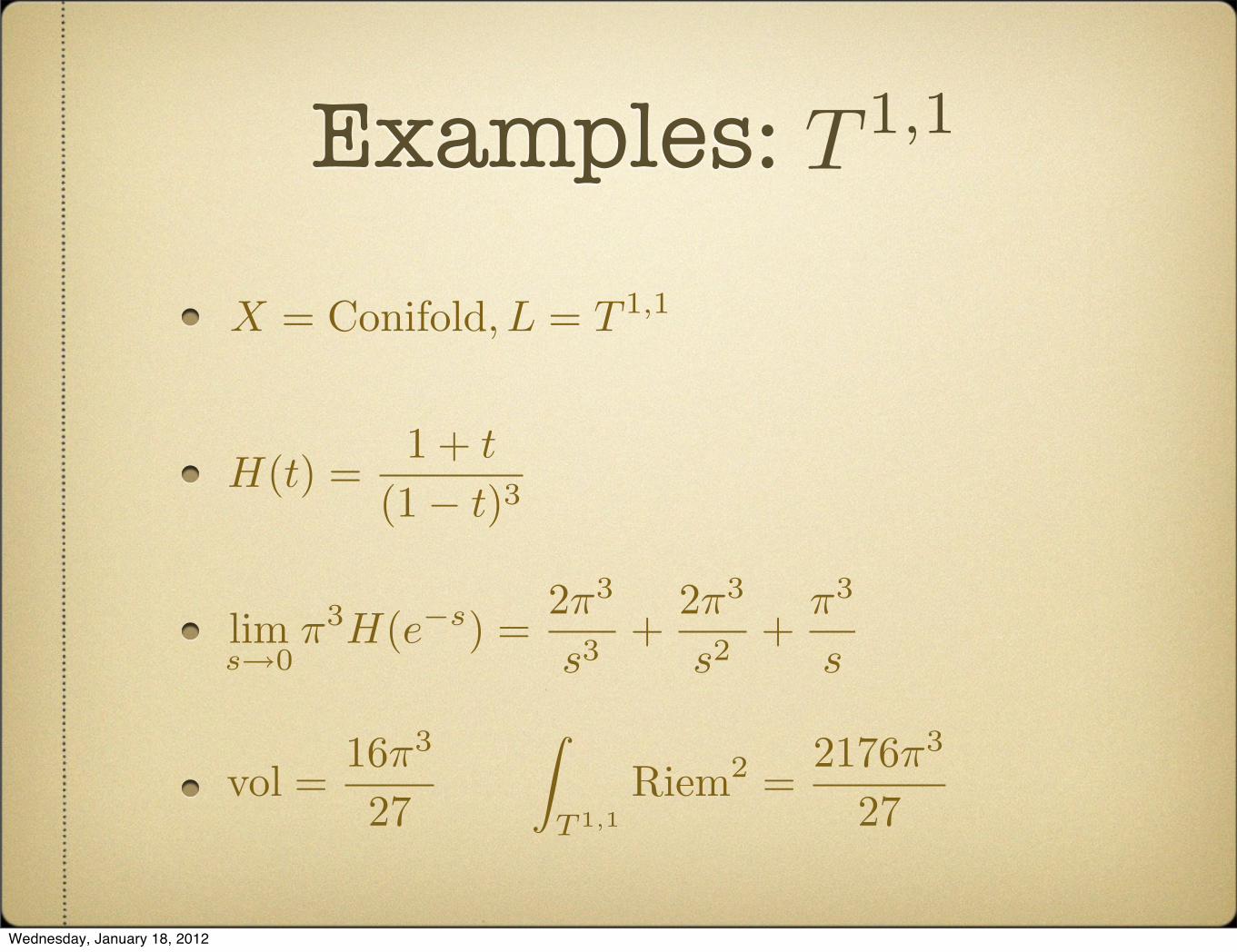
Examples:

vol =16π3

27

�

T 1,1Riem2 =

2176π3

27

H(t) =1 + t

(1− t)3

X = Conifold, L = T 1,1

lims→0

π3H(e−s) =2π3

s3+

2π3

s2+

π3

s

T 1,1

Wednesday, January 18, 2012

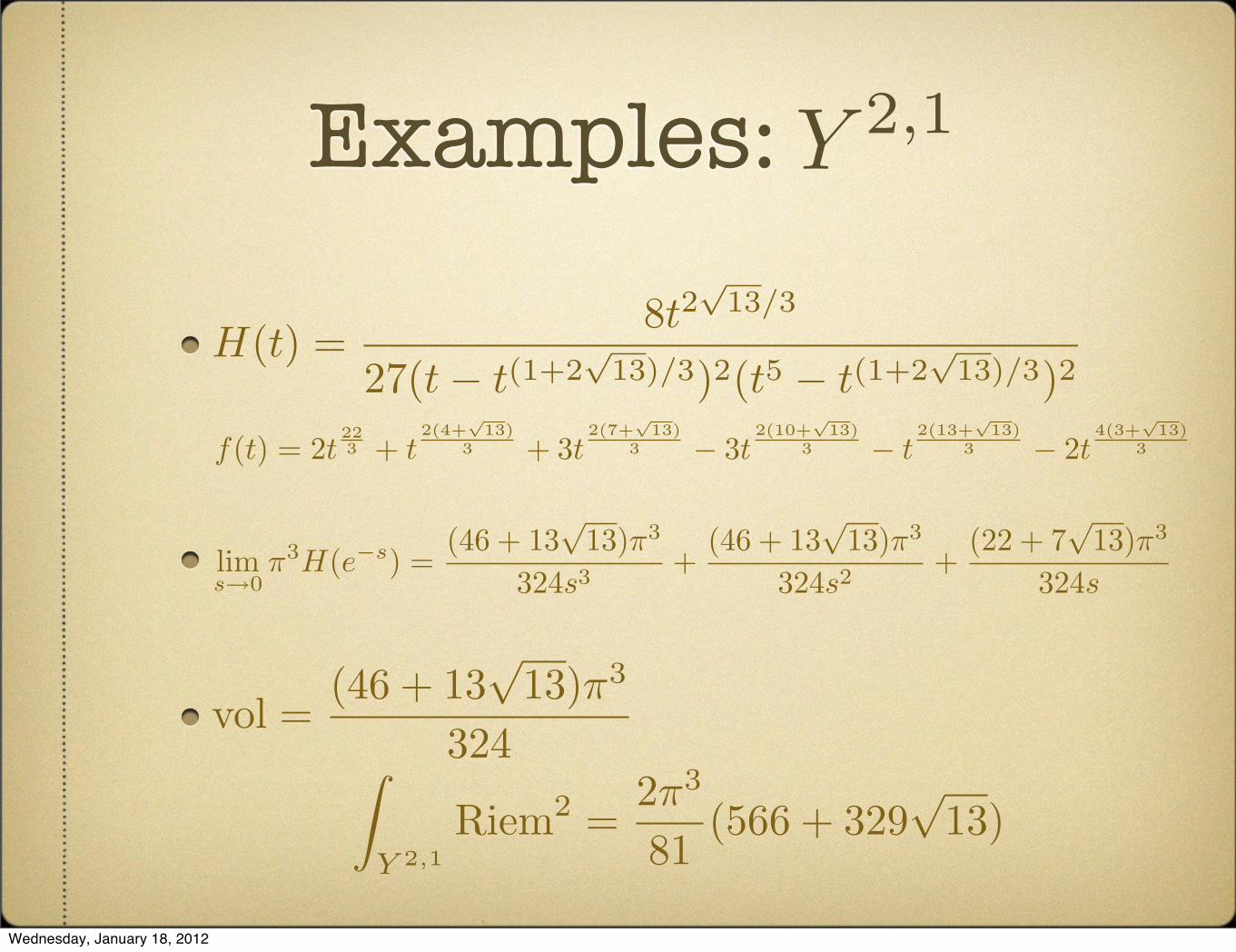
Examples:

�

Y 2,1Riem2 =

2π3

81(566 + 329

√13)

vol =(46 + 13

√13)π3

324

lims→0

π3H(e−s) =(46 + 13

√13)π3

324s3+

(46 + 13√

13)π3

324s2+

(22 + 7√

13)π3

324s

H(t) =8t2√

13/3

27(t− t(1+2√

13)/3)2(t5 − t(1+2√

13)/3)2

f(t) = 2t223 + t

2(4+√

13)3 + 3t

2(7+√

13)3 − 3t

2(10+√

13)3 − t

2(13+√

13)3 − 2t

4(3+√

13)3

Y 2,1

Wednesday, January 18, 2012

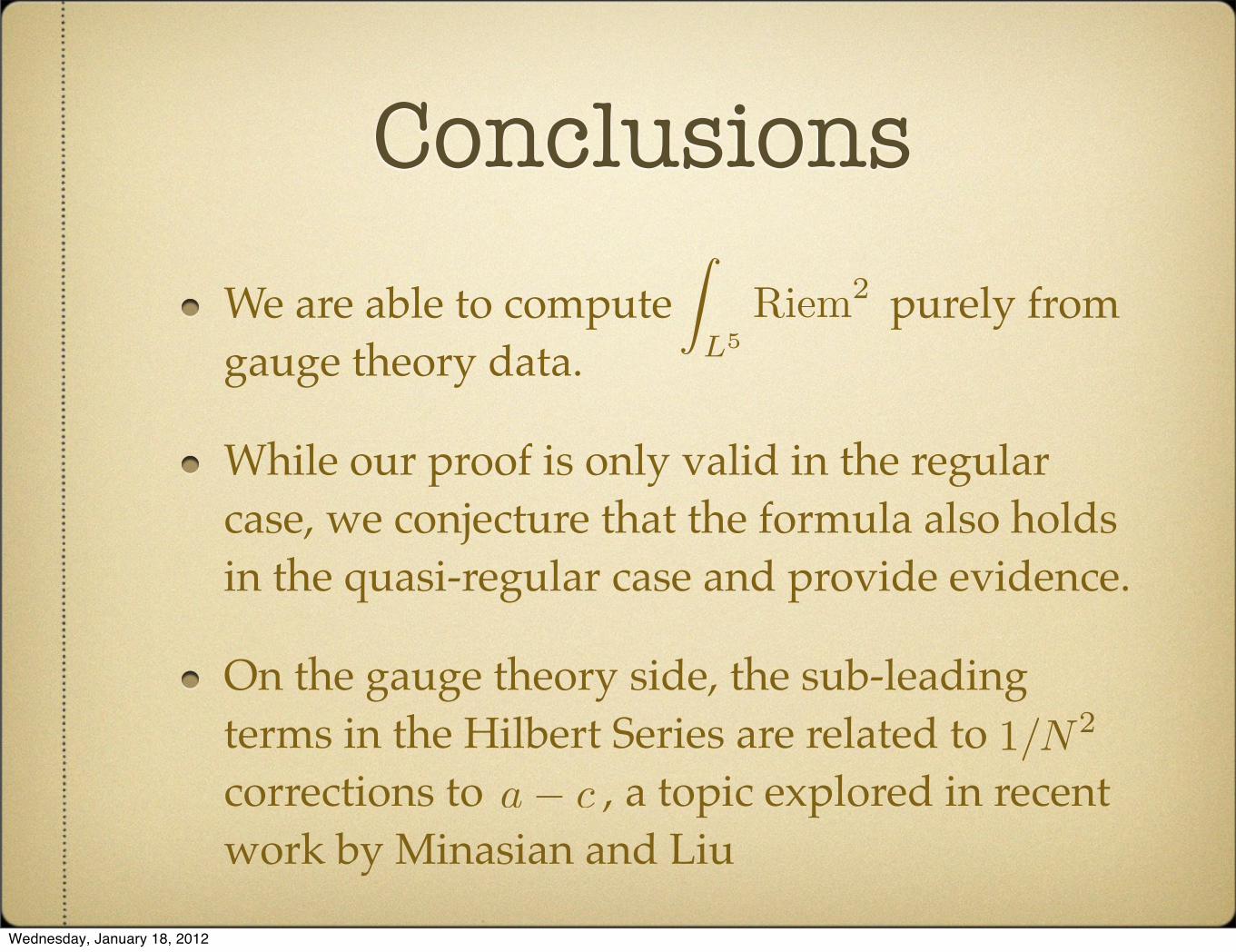
ConclusionsWe are able to compute purely from gauge theory data.

While our proof is only valid in the regular case, we conjecture that the formula also holds in the quasi-regular case and provide evidence.

On the gauge theory side, the sub-leading terms in the Hilbert Series are related to corrections to , a topic explored in recent work by Minasian and Liu

�

L5Riem2

a− c1/N2

Wednesday, January 18, 2012

Future DirectionsGeneralize the proof to the quasi-regular case by properly treating singular points.

The fact that the sub-leading terms can be written purely in terms of 5d quantities hints at a direct 5d proof.

Extend to Generalized Complex Geometry, as recently considered by Gabella and Sparks.

Understand relation to higher curvature corrections to bulk action.

Wednesday, January 18, 2012