DO WE FIND HIGH ENERGY PHYSICS INSIDE(ALMOST) EVERY SOLID OR FLUID AT LOWTEMPERATURE?

H. B. Nielsena and M. Ninomiyab

aNiels Bohr Institute, University of Copenhagen,17 Belgdamsvej, DK 2100 Copenhagen φ, Denmark

bAdvanced Mathematical Institute Osaka-city University, Sugimoto 3-3-138, Sumiyoshi-ku Osaka, 1558-8585,Japanand Yukawa Institute for Theoretical Physics, Kyoto University Kyoto. 606-8502, Japan

Abstract: It is an old idea of ours (H. B. Nielsen “Dual Models” section 6 “Catastrophe TheoryProgram” Scottish University Summer School 1976) that a most general material with only translationsymmetry, but otherwise no symmetries should generically (in general) have some small regions in quasimomentum space, where you “see” an approximate Weyl equation behavior. The Weyl equation is therelativistic equation for a (left handed) neutrino. This remark means that one could imagine, thatthere were behind the Standard Model of High energy physics, a very general crystal model withvery little symmetry. Even for the Yang Mills or electrodynamics types fields a similar philosophy ispossible. There are though some problems with this solid-state type of model beyond the Standardmodel, for which we thought have some remedy by means of homolumo gap effects.

By making use of relativistic quantum field theory on the lattice we predicted theoretically veryhigh magneto-conduction due to Adler-Bell-Jackiw chiral anomaly effect – so called Nielsen-Ninomiyaeffect (or mechanism) in gapless parity violating material. Nowadays this kind of material such aschiral or Weyl semimetal and the effect are detected by experiments.

arX

iv:1

806.

0450

4v1

[ph

ysic

s.ge

n-ph

] 7

Jun

201

8

Introduction

The authors, in particular H. B. N. have through many years the dream, that it is not important whatthe (most) fundamental laws of Nature might be, because almost certainly the same effective lawswould come out anyway: This philosophy is called “Random Dynamics”.

Inside a piece of matter - crystal, glass, ... - one should then at very low temperature accordingto this dream find the Standard Model.

Recently one is about to find Cases of Relativity-behaving Quasi-particles: A material, e.g.graphene, with such simulations of relativistic particles as we talk about.

Materials with relativistic particles simulated as quasiparticles may be very applicable to say highconductivity purposes,...

Some of our publications:

• H. B. Nielsen and M. Ninomiya, “No Go Theorem for Regularizing Chiral Fermions,” Phys. Lett.105B, 219 (1981).

• H. B. Nielsen and M. Ninomiya, “Absence of Neutrinos on a Lattice, 1. Proof by homotopytheory” Nucl. Phys. B 185, 20 (1981).

• H. B. Nielsen and M. Ninomiya, “Absence of Neutrinos on a Lattice. 2. Intuitive TopologicalProof,” Nucl. Phys. B 193, 173 (1981).

• As for the initiation of Random Dynamics, See “Fundamentals of Quark Models”. Proceedings:17th Scottish Universities Summer School in Physics, St. Andrews, Aug 1976, I.M. Barbour, A.T.Davies (Glasgow U.);1977 - 588 pages; Edinburgh: SUSSP Publ. (1977);Conference: C76-08-01;Contributions: Dual Strings, Holger Bech Nielsen (Bohr Inst.). Aug 1974, 71 pp.;NBI-HE-74-15In the last section the idea of “Random Dynamics ” is introduced based on finding Weyl equationin “whatever”.

The present paper consists as part I and part II.The part I: Relativity Theory found in solid state.andThe part II “What comes beyond Topological Insulator – Nielsen-Ninomiya Effect

(or Mechanism) due to ABJ Anomaly –”Part I: Relativity-Theory found in Solid State Physics

I-1 Introduction

I-2 Automatic: a pet-thought: Natural laws come by themselves! (“Random Dynamics”)

I-3 General: A very general world with (only) momentum conservation.

I-4 Graphene: Example Graphene.

I-5 Heusler: Half-metals, Heusler compounds.

I-6 Wang: Thoughts about making materials having models of relativistic particles inside.

I-7 Doubling: Nielsen - Ninomiya theorem about doubling of such relativistic particles unavoidablyon the lattice. great future; hope of seeing high energy physics in low temperature materials notout, but not quite finished. material simulates relativistic quantum field theory.

– 1 –

I-8 Further: Further Developments of our “Random Dynamics”

I-9 Conclusion for part I

The part II: What comes beyond Topological Insulator –Nielsen-Ninomiya Effect (or Mechanism)due to ABJ Anomaly

II-1 : Introduction

II-2 : 1+1 dimensional Example

II-3 : 3+1 dimensional case Weyl (or chiral) Fermion Adler-Bell-Jackiw Anomaly

II-4 : Parity non-invariant, Zero-gap material

II-5 : Transfer from Left- to Right- comes by Adler-Bell-Jackiw anomaly

II-6 : Further arguments

II-7 : Conclusions

Appendix A : Necessary properties of quantum field theory in this paper

Appendix B : Adler-Bell-Jackiw anomaly in continuum spacetime

I-2 Automatic

Our Old Work in 1976: Dreams Laws of Nature Automatic"Dual Strings. Fundamentals of Quark Models." by H. B. Nielsen, in Scottish University Summer

School in Physics, St. Andrews, 1976 (There H.B.N. still mainly is talked on String theory, but at theend a general (fermion) Hamiltonian is studied.)

Assumed was translational invariance, at least with respect to a lattice say, and thus a (quasi)momentum conservation, but with respect to the “internal degrees of freedom” there is a very gen-eral theory, though assuming there being essentially a finite (discrete). system of states(representingpossibly spin and band degrees of freedom.).

(Trivial) Generic Considerations on Fermion Dispersion relations (1976). We ignore allconservation laws except for

• Energy conservation and Hamiltonian development.

• Momentum Conservation.

• Particle (number) conservation.

• Free approximation (first).

• Smoothness, (so that e.g H(~p) is differentiable and continuous as function of ~p.)

• Generic: i.e. no fine-tuned values of parameters,

– 2 –

and consider a single particle equation:

i∂

∂tψ(~p, t) = H(~p)ψ(~p), (0.1)

where for each value of the momentum ~p the H(~p) is a Hermitian matrix.Relativity and Dimensionality of Space time being 3+1 come out Automatically!A priori - with no fine-tuning (=generically) - the Fermi surface would put itself at separate

eigenvalues; but if for some reason ( e.g. “homlumo-gap effect”) the Fermi-level were just where n = 2

levels meet, then in a small neighborhood the shape of the dispersion relations would be given bytaking H(p) to be n× n = 2× 2. We then Taylor expand

H(~p) ≈ H(~p0) +∑a,µ

σaV µa pµ + ... (0.2)

where σa are the Pauli-matrices and the unit matrix σ0 = 1. The “vierbein” V µa is a set of expansioncoefficients for H(~p) as function of the components pµ (strictly speaking µ =1,2,3; here).

Hermitian matrix, Provided Fermi-level at Degeneracy n = 2 leads to Weyl Equationin 3+1 Dimensions.

In the old days we argued that in a general physics universe the Hubble expansion would finallylead to the Fermi-level approaching an n = 2 degenerate levels energy; but now H. B. N.’s Zagreb group- I.Andric, L. Jonke, D. Jurman, and HBN - have studied in general, what is called “Homolumo-gapEffect” meaning the by Jahn and Teller[1] first proposed effect, that the electrons filling the Fermi-seawould back react such as to increase the homolumo gap between the lowest unoccupied (LUMO) andthe highest occupied (HOMO) state. This effect goes in the direction to make metals not occur, andmake every materials become an insulator, but the gapless semiconductor may be too hard for thehomolumo-gap effect to dispense with.

Note that this hope for getting automaticly a Weyl-equation like theory had, when using justHermitean Hamiltonian marices and looking at the n = 2 degeneracy possibility, the consequence thatthere came only three spatial dimensions functioning the relativistic way, because there were only 3Pauli matrices. Somehow arguing that the dimensions for which there are no Pauli matrices will leadto essentially zero velocity for the fermion/quasi-electron in these directions and that such dimensionswill not be observed, we have come to 3+1 dimensions as an additional prediction from the verygeneral starting theory!

With time-reversal symmetry imposed dimension prediction gets modified.

Symmetry Square Pauli M. Dimension FieldTP (TP )2 = 1 σx, σz 2+1 Real- - σx, σy, σz 3+1 Complex

TP (TP )2 = −1 5 of them 5+1 Quaternions

Table 1. The symmetry assumed in line 1 and 3 is the combination of time reversal T and parity P toTP, which leaves the momentum ~p invariant but is an antilinear operator effectively conjugating the complexnumbers in the matrix. If then Fermi-level falls at n = 2 degenerate levels in addition to the Kramers-Kronigdoubling in the 3rd case, one gets by Taylor expanding the 2×2 resolved into Pauli-matrices, and a generalizedWeyl equation results corresponding to the in fourth column denote space + time dimensions. Actually theeffective theory is naturally written in terms of the in column 5 mentioned division-algebra(= field).

Fundamentally in many Dimensions, but in Most dimensions the Fermion Run withZero Velocity, we Ignore them.

– 3 –

In the for fundamental physics ideal situation of no extra T or TP symmetry the Hamiltonianmatrix H(~p) is just a generic(∼ random) Hermitian matrix (with complex matrix elements), and itpredicts at the two levels degenerate point - hoped to be favored at the Fermi-surface by either Hubbleexpansion or homolumo-gap-effect - that the Fermion only moves with appreciable velocity in as manyspatial dimensions as there are Pauli-matrices. We hope that the dimensions in which the velocitygets zero, can/shall be ignored. If the zero-velocity dimensions are ignored, then we have remarkableagreement:

The number of dimensions in which the generic double degeneracy neighborhood has the fermionsmove just corresponds to experimental number of dimensions 3+1 and to having relativity and rota-tional invariance!

If TP (or T) is good symmetry and (TS)2 = 1thenH(~p) must have real matrix elements.This is the case in which we in a crystal - with PT symmetry say - completely ignore the usual

spin as being decoupled so as to be totally ignored.In this case we get the effective dimensionality, if we ignore the zero-velocity directions:

2 + 1This means that the relativistic effective fermion should appear “generically” (automatically) even

in only 2 spatial dimensions.With Genuine Spin= 1

2 Electrons and Unbroken Time reversal, the “Quaternion Case” If T or TPgood symmetries, and spin 1

2 included, then T 2 = (TP )2 = −1 we have generally doubling of all levelsaccording to Kramers-Kronig rule.[2]

So double degeneracy is already there generally and nothing special. In this case we shall thereforeinstead consider that we can get 4 times degenerate levels sporadically. If we go to such a 4-timesdegenerate point in momentum space, we could elegantly go to a quaternion 2×2 matrices (quaternionsare writable as 2× 2 complex matrices, so that 2× 2 quaternion matrices can be equivalent to 4× 4

complex matrices with some restriction. Dimension of non-zero velocity directions:

5 + 1I-3 Graphene

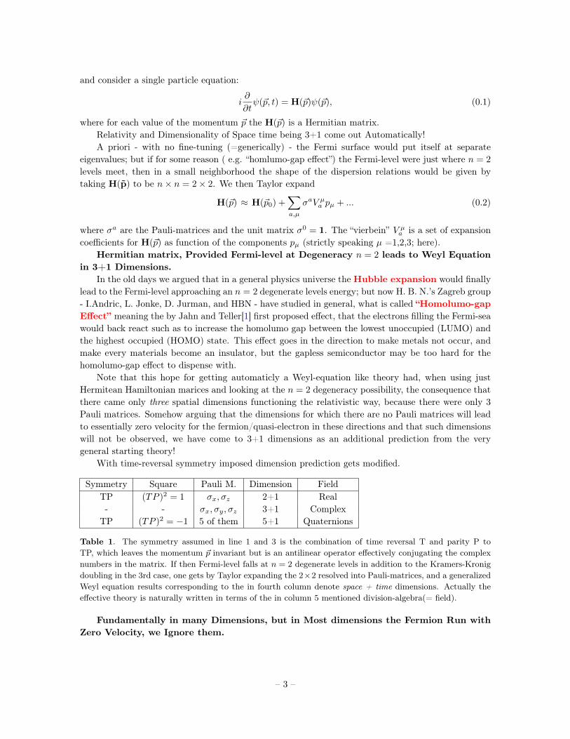
Graphene denotes the layer of carbon like the ones in graphite taken as seperate, i.e. it is 2(space)dimensionalmaterial. The quasi electrons running in the graphene layers actuall do show dispersion relations be-having how we above argued for the case with time reversal but ignoring the spin leading to theeffective space time dimension 2+1.

On the following picture one sees the lattice structure of graphene:

– 4 –

(2+1)-dimensional Example is Graphen.

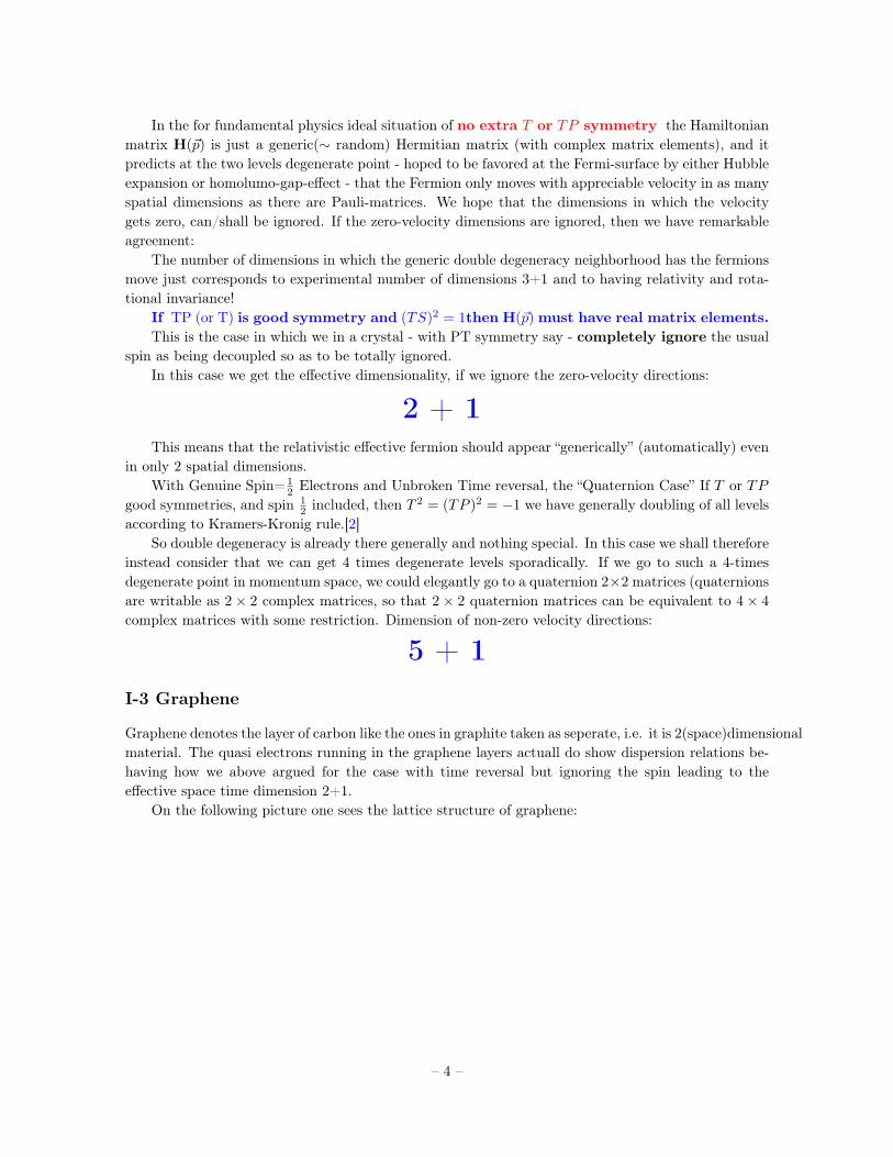
The next figure is supposed to generally illustrate a metal, an insulator and a material with a Dirac-likequasi particle (on the figure graphen).

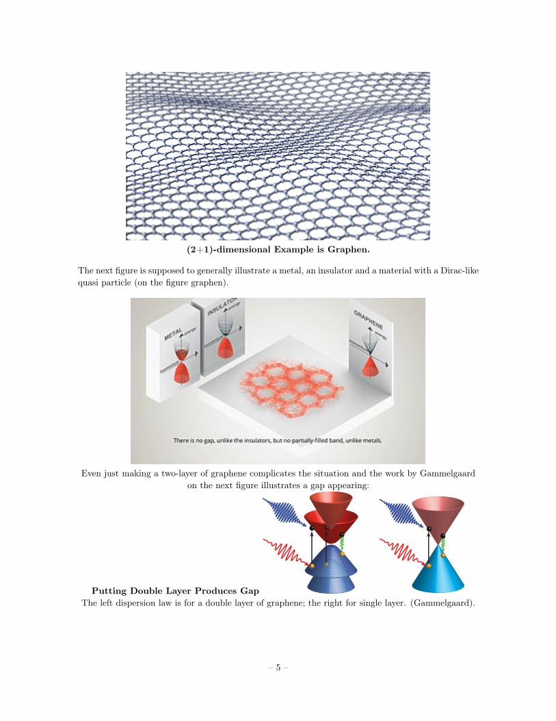
Even just making a two-layer of graphene complicates the situation and the work by Gammelgaardon the next figure illustrates a gap appearing:

Putting Double Layer Produces GapThe left dispersion law is for a double layer of graphene; the right for single layer. (Gammelgaard).

– 5 –

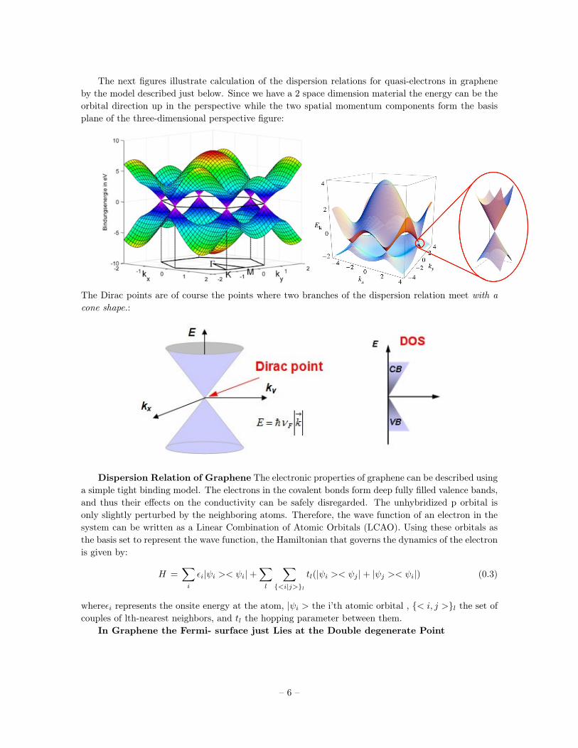
The next figures illustrate calculation of the dispersion relations for quasi-electrons in grapheneby the model described just below. Since we have a 2 space dimension material the energy can be theorbital direction up in the perspective while the two spatial momentum components form the basisplane of the three-dimensional perspective figure:

The Dirac points are of course the points where two branches of the dispersion relation meet with acone shape.:

Dispersion Relation of Graphene The electronic properties of graphene can be described usinga simple tight binding model. The electrons in the covalent bonds form deep fully filled valence bands,and thus their effects on the conductivity can be safely disregarded. The unhybridized p orbital isonly slightly perturbed by the neighboring atoms. Therefore, the wave function of an electron in thesystem can be written as a Linear Combination of Atomic Orbitals (LCAO). Using these orbitals asthe basis set to represent the wave function, the Hamiltonian that governs the dynamics of the electronis given by:

H =∑i

εi|ψi >< ψi|+∑l

∑{<i|j>}l

tl(|ψi >< ψj |+ |ψj >< ψi|) (0.3)

whereεi represents the onsite energy at the atom, |ψi > the i’th atomic orbital , {< i, j >}l the set ofcouples of lth-nearest neighbors, and tl the hopping parameter between them.

In Graphene the Fermi- surface just Lies at the Double degenerate Point

– 6 –

So in graphene by symmetry one really get a simulation of a 2+1 dimensional massless Weyl/Diracfermion, also w.r.t. the placing of the fermi surface.

If we think of just the generic case of a very general theory there will typically be no reason whythe fermi surface should be just at the Weyl point (with the double degeneracy).

We have, however, speculated on two mechanisms, which might make the fermi-surface be driventowards the degeneracy point:

• If the world in question has a strong Hubble expansion, then filled states above the degeneracypoint would be gradually emptied and holes below the degeneracy point would be also graduallybe expanded away/attenuated.

• “Homolumo-gap-effect” - meaning that the fermions act back onto the various degrees of freedomthat can be adjusted in the lattice in which the fermions run. This back action will be so asto in the ground state arrange to lower the energies of filled fermi states. Thereby arise the socalled Homolumo-gap, or rather it gets expanded by this back action “homolumo-gap-effect”. Inthe case that we have degeneracy point that is somehow topologically stabilized, as one mightsay of the Weyl points discussed here, it may not be possible for the homolumo-gap-effect toreally produce a gap. In stead we expect that it will only bring the fermi surface to coincidewith the degeneracy point; that would namely lower the filled states as much as possible withthe “topological ensurance” of the degeneracy point.

I-4 Heusler

Heusler Compound Mn2CoAl is a Spin Gapless Semicondutor:Siham Oardi, G.H. Fecher, C. Felser and J. Kübler (arXiv:1210.0148v1 [cond-mat.mtrl-sci], 29 Sep.

2012.) investigated theHeusler compound Mn2CoAl. They gave the article the name Realizationof spin gapless semiconductors: the Heusler compound Mn2CoAl.

In halfmetallic ferromagnets you have so to speak metal as far as the electrons with one directionof the spin is concerned, but insulator w.r.t. to the elctrons with the opposite spin direction. Now itmay further happen that we instead of the metallic we get a gapless semiconductor, namely if we havea degeneracy point as we discussed above. Once there is effectively only one spin of the electron oneescapes the time reversal symmetry. Thus in such halfmettals there is a better chance to find Weylpoints.

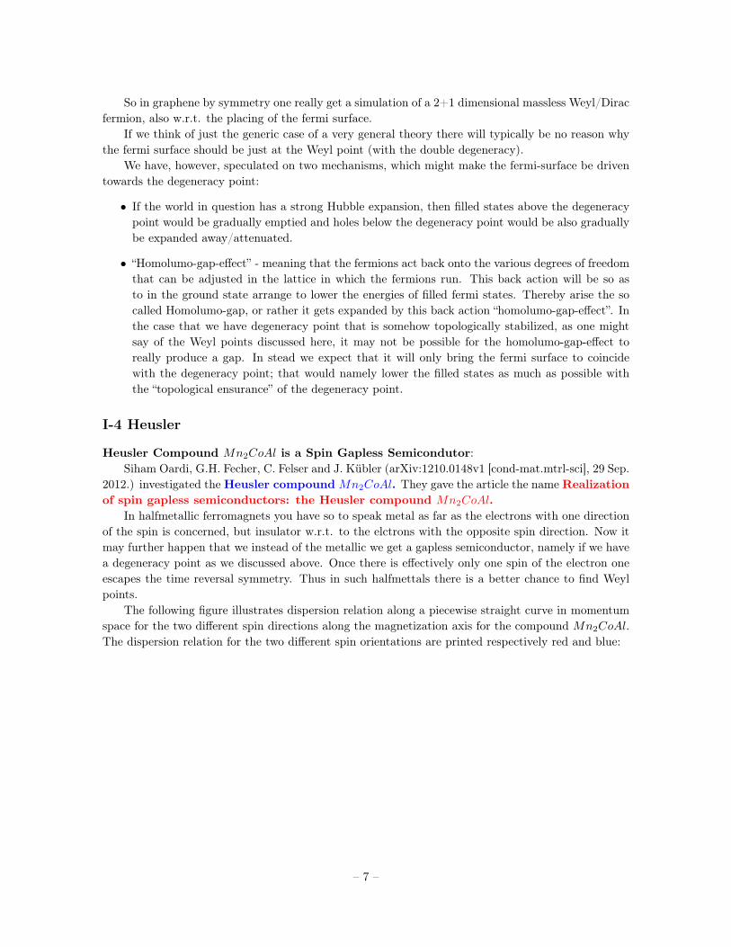
The following figure illustrates dispersion relation along a piecewise straight curve in momentumspace for the two different spin directions along the magnetization axis for the compound Mn2CoAl.The dispersion relation for the two different spin orientations are printed respectively red and blue:

– 7 –

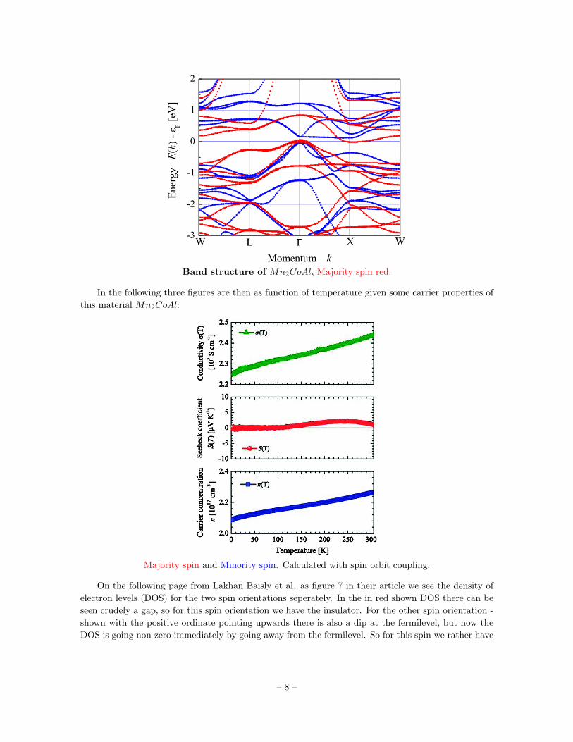
Band structure of Mn2CoAl, Majority spin red.

In the following three figures are then as function of temperature given some carrier properties ofthis material Mn2CoAl:

Majority spin and Minority spin. Calculated with spin orbit coupling.

On the following page from Lakhan Baisly et al. as figure 7 in their article we see the density ofelectron levels (DOS) for the two spin orientations seperately. In the in red shown DOS there can beseen crudely a gap, so for this spin orientation we have the insulator. For the other spin orientation -shown with the positive ordinate pointing upwards there is also a dip at the fermilevel, but now theDOS is going non-zero immediately by going away from the fermilevel. So for this spin we rather have

– 8 –

the gapless semiconductor behavior.

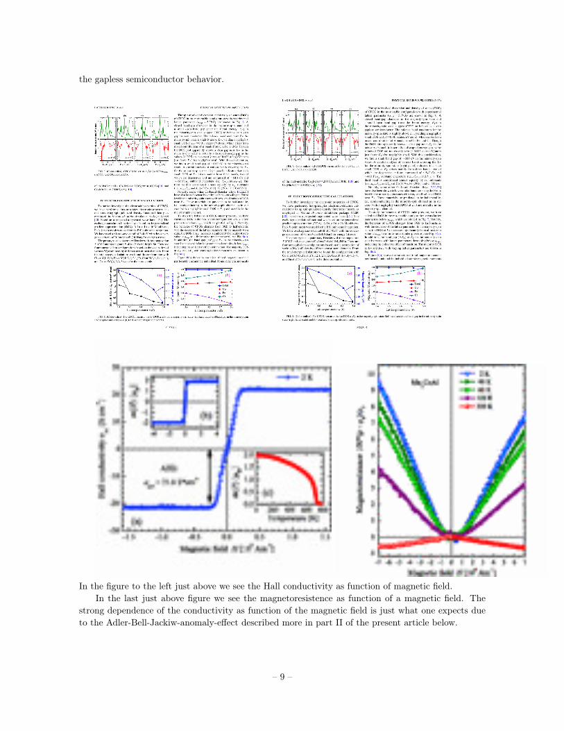
In the figure to the left just above we see the Hall conductivity as function of magnetic field.In the last just above figure we see the magnetoresistence as function of a magnetic field. The

strong dependence of the conductivity as function of the magnetic field is just what one expects dueto the Adler-Bell-Jackiw-anomaly-effect described more in part II of the present article below.

– 9 –

These figures are fromSiham Ouardi et al. “Realization of Spin Gapless Semiconductors: The Heusler Compound

Mn2CoAl” DOI: 10.1103/PhysRevLett.110.100401

Zero Gap Material with Quadratic Energy Dispersion (this is by fine tuning) HgTe is oneof the few materials wherin this quadratic dispersion law zero gap has been found, since 1950’s.

Pb1−xSnxTe, Pb1−xSnxSeandBixSb1−x are zero-gap materials (with quadratic disp.).But really one - Wang, Dou, and Zhang - expects that all narrow gap semiconductors by some

doping or pressure could be tuned to have zero gap (with quadratic dispersion law). Then they callfor finding a non-toxic material of this kind.

I-5 Wang

Physical Chemistry; Chemical PhysicsControllable electronic and magnetic properties in a two-dimensional germanene heterostructure

Run-wu Zhang, Wei-xiao Ji, Chang-wen Zhang,* Sheng-shi Li,b Ping Li, Pei-ji Wang, Feng Lia andMiao-juan Rena Author affiliations Abstract

The control of spin without a magnetic field is one of the challenges in developing spintronic devices.Here, based on first-principles calculations, we predict a new kind of ferromagnetic half-metal (HM)with a Curie temperature of 244 K in a two-dimensional (2D) germanene Van der Waals heterostructure(HTS). Its electronic band structures and magnetic properties can be tuned with respect to externalstrain and electric field. More interestingly, a transition from HM to bipolar-magnetic-semiconductor(BMS) to spin-gapless-semiconductor (SGS) in a HTS can be realized by adjusting the interlayerspacing. These findings provide a promising platform for 2D germanene materials, which hold greatpotential for application in nanoelectronic and spintronic devices.

I-6 Doubling

Nielsen-Ninomiya’s No-go theoremThe authors are very proud of, that we have shown a theorem saying:When one makes the mentioned “relativistic fermions of Weyl-type” (=chirale fermion)

on a lattice (so e.g. in a crystal) then you always get equally many right-spinning andleft-spinning Weyl-type particle(species).

This theorem is a great challenge for those wanting to make a lattice model (with calculationalpurposes) for a theory with massless (or almost massless) quarks, let alone the Standard Model.

By having 3 K +3 K′ Dirac-points of Compensating Handedness Our Doubling The-orem Realized in Graphene.

– 10 –

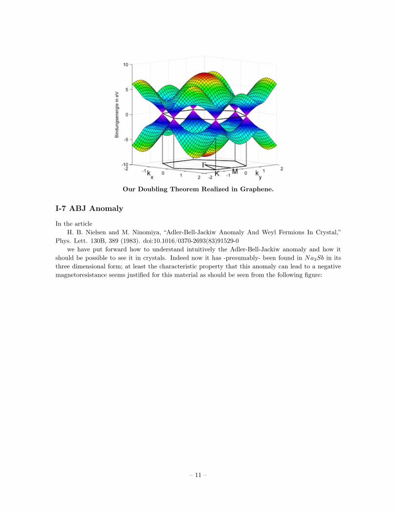
Our Doubling Theorem Realized in Graphene.

I-7 ABJ Anomaly

In the articleH. B. Nielsen and M. Ninomiya, “Adler-Bell-Jackiw Anomaly And Weyl Fermions In Crystal,”

Phys. Lett. 130B, 389 (1983). doi:10.1016/0370-2693(83)91529-0we have put forward how to understand intuitively the Adler-Bell-Jackiw anomaly and how it

should be possible to see it in crystals. Indeed now it has -presumably- been found in Na3Sb in itsthree dimensional form; at least the characteristic property that this anomaly can lead to a negativemagnetoresistance seems justified for this material as should be seen from the following figure:

– 11 –

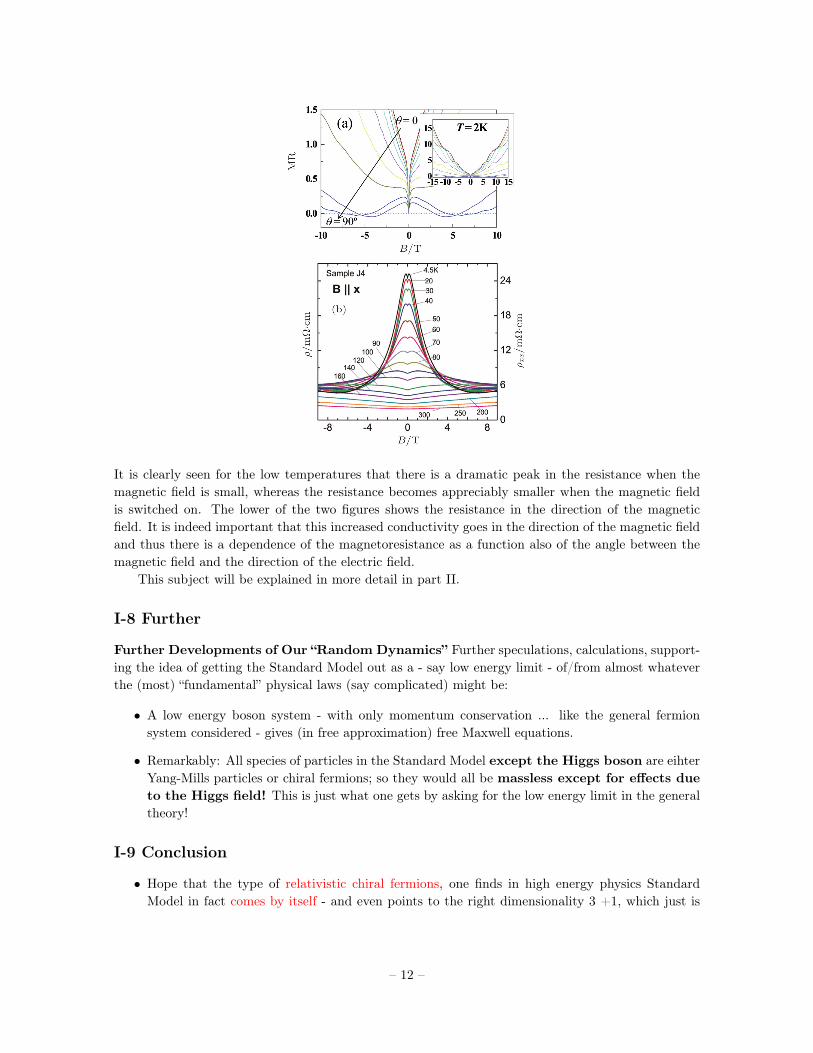
It is clearly seen for the low temperatures that there is a dramatic peak in the resistance when themagnetic field is small, whereas the resistance becomes appreciably smaller when the magnetic fieldis switched on. The lower of the two figures shows the resistance in the direction of the magneticfield. It is indeed important that this increased conductivity goes in the direction of the magnetic fieldand thus there is a dependence of the magnetoresistance as a function also of the angle between themagnetic field and the direction of the electric field.

This subject will be explained in more detail in part II.

I-8 Further

Further Developments of Our “Random Dynamics” Further speculations, calculations, support-ing the idea of getting the Standard Model out as a - say low energy limit - of/from almost whateverthe (most) “fundamental” physical laws (say complicated) might be:

• A low energy boson system - with only momentum conservation ... like the general fermionsystem considered - gives (in free approximation) free Maxwell equations.

• Remarkably: All species of particles in the Standard Model except the Higgs boson are eihterYang-Mills particles or chiral fermions; so they would all be massless except for effects dueto the Higgs field! This is just what one gets by asking for the low energy limit in the generaltheory!

I-9 Conclusion

• Hope that the type of relativistic chiral fermions, one finds in high energy physics StandardModel in fact comes by itself - and even points to the right dimensionality 3 +1, which just is

– 12 –

the right one-; but there are a couple of “small” problems (different species of particles have infirst go different “maximal” velocities)

• Now adays the phenomenon is about being found in real materials, graphene etc. One can makerelativity models chemically

It should be especially stressed that the negative magneto-resistance due to the Adler BellJackiw anomaly has been seen in Na3Sb.

– 13 –

II. What comes beyond Topological Insulator ?–“Nielsen-Ninomiya Effect” due to Adler-Bell Jackiw chiral Anomaly–

II-1 Introduction

In part I we mainly argued about “Gapless Semiconductor” “Topological Insulator” and this subjecthas been very rapidly developing presently.

We now, in this part II, argue chiefly a new application of relativistic quantum field theory.Specifically, We investigate in condensed matter (in nano-scale∼= 10−9m) how the Relativistic Quantumfield theory Effect can appear and can be detected in material science.

Theoretically this effect was predicted already 35 years ago in 1983 by the present authors

• (H. B. N and M. N.) in a High Energy Theoretical Physics journal, Physics Letters B Vol. 130,issue 6 p 389 (1983), entitled “The Adler-Bell-Jackiw anomaly and Weyl Fermions in a Crystal”.

• Prior to the above paper one of the authors (M. N) was invited to give talks in the InternationalWorkshop on “Lattice Field Theory” in Saclay, Paris and Subsequently held XXI InternationalConference on High Energy Physics, Paris July 26-31, 1982 (so called “Rochester Conferenceseries”), where he talked about Weyl fermions on lattices and the ABJ-anomaly.

In solid material there offen appears crystal lattice structure. Thus we are forced to use lattice fieldtheory which has been well developped in high energy physics. In this formulation the crucial factsfor us are the following:

Suppose At each lattice site we put one Weyl fermion e.g. ΨL (Left-handed one).Our Nielsen-Ninomiya Theorem states that there should appear equally many right handed and

left handed Weyl fermions - looking in momentum space at different momentum values -. In thesimplest construction resulting from just “naively” replacing derivatives by differences on the latticeour theorem is implemented by there appearing 2d species (d: space dimension). Therefore in 3 spacedimensions it turs out that there should be 8 species of Weyl (or chiral) fermions. Furthermore 4 ofthem are left-handed ΨL and rest 4 species are right-handed ΨR chiral fermions.

That is to say on the lattice there should be pairwise (left-handed and right-handed) chiralfermions. Therefore we are not able to construct chiral theory with for instance only one handedfermion on the lattice. Thus it leads to the very important consequence in high energy physics. In re-ality the Standard Model or, unified model of, weak and electromagnetic interactions called “Glashow-Salam-Weinberg model”, or “Standard Model” of Weak and Electromagnetic Interaction cannot beconstructed on the lattice! The reason is that in the Standard Model all the fermions are left-handedchiral fermions, while no right-handed fermion at all. The experimental results performed so far areall well in agreement with the standard model predictions.

If one takes serious the proposal of a new law of nature by one of us and various collaborators,“Multiple Point Principle”, one can even claim an indication for, that the Standard Model contraryto the expectation of many of our colleagues, should be valid up to an energy scale of the order of1018GeV (rather close to the Planck scale):

One of the authors (H. B. N.) made together with C. D. Froggatt a theoretical calculation ofmH with recourse to the just mentioned “multiple point principle (MPP)”. The value is in very goodagreement with experimental value at LHC (Large Hadron Collider in CERN, Geneva) mH ∼ 125GeV.

See e.g. H. B. Nielsen and M. Ninomiya “Degenerate vacua from unification of second law ofthermodynamics with other laws; The derivation of Multiple point principle” Int. J. Mod. Phys. A23

– 14 –

(2008) 919 DOI: 10.1142/S02177510839682, in which an argument for among other things is givenMPP from a model with the action taken to be complex rather than real as it is normal.

If the Standard Model shall as from this suggestion from Multiple Point Principle etc. be validonly with tiny corrections if any almost up to the Planck scale, it would be even more mysteriousthat we could not put it on a lattice because of its chiral particles. Really we could -it looks -hardlyregularize it with any sensible cut off! Quite a mystery. [3]

2) ABJ anomaly on a latticeCondensed matter researchers except for high energy physicists (including some nuclear theorists),

may not have heard of the Adler-Bell-Jackiw or chiral anomaly. Therefore we briefly explained ABJanomaly in continuum space in Appendix A.

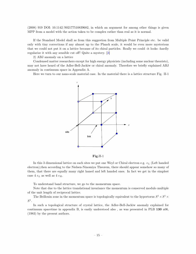
Here we turn to our nano-scale material case. In the material there is a lattice structure Fig. II-1

Fig.II-1

In this 3 dimensional lattice on each sites we put one Weyl or Chiral electron e.g. eL (Left handedelectron),then according to the Nielsen-Ninomiya Theorem, there should appear somehow so many ofthem, that there are equally many right haned and left handed ones. In fact we get in the simplestcase 4 eL as well as 4 eR.

To understand band structure, we go to the momentum space.Note that due to the lattice translational invariance the momentum is conserved modulo multiple

of the unit length of reciprocal lattice.The Brillouin zone in the momentum space is topologically equivalent to the hypertorus S1×S1×

S1.In such a topological structure of crystal lattice, the Adler-Bell-Jackiw anomaly explained for

continuum spacetime in appendix B, is easily understood also , as was presented in PLB 130 n06,(1983) by the present authors.

– 15 –

II-2 1 + 1 dimensional example

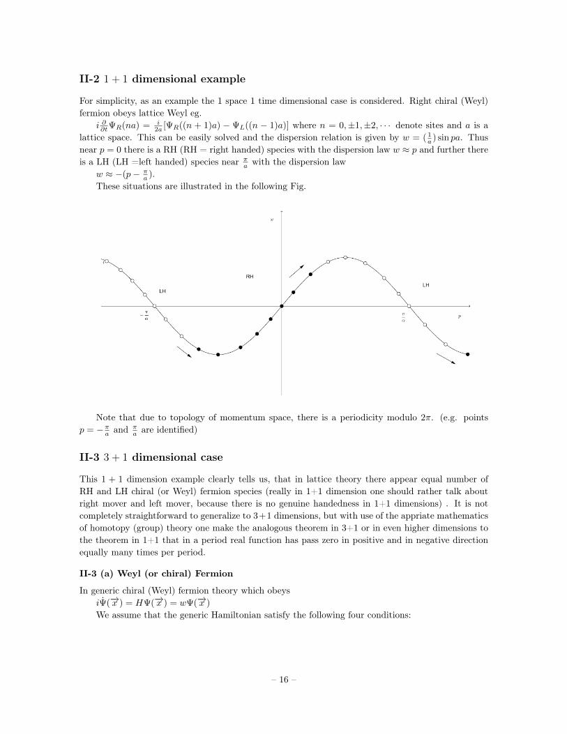
For simplicity, as an example the 1 space 1 time dimensional case is considered. Right chiral (Weyl)fermion obeys lattice Weyl eg.

i ∂∂tΨR(na) = i2a [ΨR((n + 1)a) − ΨL((n − 1)a)] where n = 0,±1,±2, · · · denote sites and a is a

lattice space. This can be easily solved and the dispersion relation is given by w = ( 1a ) sin pa. Thus

near p = 0 there is a RH (RH = right handed) species with the dispersion law w ≈ p and further thereis a LH (LH =left handed) species near π

a with the dispersion laww ≈ −(p− π

a ).These situations are illustrated in the following Fig.

Note that due to topology of momentum space, there is a periodicity modulo 2π. (e.g. pointsp = −πa and π

a are identified)

II-3 3 + 1 dimensional case

This 1 + 1 dimension example clearly tells us, that in lattice theory there appear equal number ofRH and LH chiral (or Weyl) fermion species (really in 1+1 dimension one should rather talk aboutright mover and left mover, because there is no genuine handedness in 1+1 dimensions) . It is notcompletely straightforward to generalize to 3+1 dimensions, but with use of the appriate mathematicsof homotopy (group) theory one make the analogous theorem in 3+1 or in even higher dimensions tothe theorem in 1+1 that in a period real function has pass zero in positive and in negative directionequally many times per period.

II-3 (a) Weyl (or chiral) Fermion

In generic chiral (Weyl) fermion theory which obeysiΨ(−→x ) = HΨ(−→x ) = wΨ(−→x )

We assume that the generic Hamiltonian satisfy the following four conditions:

– 16 –

(1) Locality of interaction in the sense that H(−→x − −→y ) → 0 as |−→x − −→y )| → large fast enoughthat the Fourie transform of H(−→x ) has continuous first derivative. (2) Translational invariance in thelattice (3) Hermiticiti of H (reality of S) (4) Furthermore an assumption is that the charge (=leptonnumber in our case) is bilinear in the fermion field.

Under these conditions in the generic H case we gave a rigorous proof in terms of the Homotopytheory in topology in 1981 (see, II-1).

II-3 (b) Adler-Bell-Jackiw anomaly on a lattice

Let us go into the Adler-Bell-Jackiw (ABJ) anomaly on the lattice in the continuum spacetime. Wereviewed this anomaly in continuum spacetime in Appendix B.

Here we argue for the lattice version of the ABJ anomaly. Firstly we as as an example let usexplain the 1 + 1 dimensional lattice Weyl (chiral) fermion. In the lattice RH chiral or Weyl electronsystem, we put on an external uniform electric field E in x-direction denoted by A1 = E in temporalgauge (A0 = 0). Then the Weyl eq. reads

i ∂∂tΨR(x) = (−i ∂∂x − A1)ΨR(x).

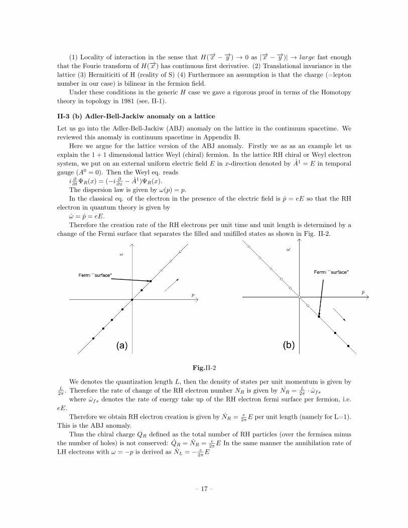
The dispersion law is given by ω(p) = p.In the classical eq. of the electron in the presence of the electric field is p = eE so that the RH

electron in quantum theory is given byω = p = eE.

Therefore the creation rate of the RH electrons per unit time and unit length is determined by achange of the Fermi surface that separates the filled and unifilled states as shown in Fig. II-2.

Fig.II-2

We denotes the quantization length L, then the density of states per unit momentum is given byL2π . Therefore the rate of change of the RH electron number NR is given by NR = L

2π · ωfswhere ωfs denotes the rate of energy take up of the RH electron fermi surface per fermion, i.e.

eE.Therefore we obtain RH electron creation is given by NR = e

2πE per unit length (namely for L=1).This is the ABJ anomaly.

Thus the chiral charge QR defined as the total number of RH particles (over the fermisea minusthe number of holes) is not conserved: QR = NR = e

2πE In the same manner the annihilation rate ofLH electrons with ω = −p is derived as NL = − e

2πE

– 17 –

This means that creation rate of the LH anti-electron is given as˙NL = e

2πE

By adding both, the anomaly of the Dirac electrons isNR + NL = e

πE, and thusQ5 = e

πE

To proceed to the 3 + 1 dimension case, we should calculate the energy levels in the presence ofan external uniform magnetic field, e.g. in the z-direction so that A2 = Hx, and Aµ = 0 otherwise.Thus we consider the equation for the two component RH electron field ΨR[

i ∂∂t − (−→p − e−→A )−→σ

]ΨR(x) = 0

This eq. can be solved by introducing an auxiliary field Φ asΨR =

[i ∂∂t + (−→p − e

−→A )−→σ

]Φ.

Thus the eq. for Φ is given by[i∂∂ − (−→p − e

−→A )−→σ

]·[i∂∂ + (−→p − e

−→A )−→σ

]Φ = 0

This eq. reduces to the harmonic oscillation tpe eq,[−( ∂

∂x′ )2 + (eH)2(x′ + p2

eH ) + (p3)2 + eHσ3]

Φ = ω2Φ with σ3 = ±1

The energy eigenvalues ω are given by the Landau levels as followsω(n, σ3, p3) = ±

[2eH(n+ 1

2 ) + (p3)2 + (eHσ3)] 1

2 with n = 0, 1, 2, · · · , except for the n = 0 andσ3 = −1 mode. Here

ω(n = 0, σ = −1, p3) = ±p3.The eigenfunction is of the formΦnσ3

(x) = Nnσ3(x)× exp(−ip2x2 − ip3x3)× exp(− 1

2eH(x′ + p2eH )2)×Hm(x′ + p2

eH )χ(σ3)

where Nnσ3 is normalization constant and χ(σ3) denotes the eigenfunctions of Pauli spin σ3 :

χ(1) =

(1

0

)and χ(−1) =

(0

1

)Thus the solution of the eq. for Two-component RH electron ΨR becomes the relations Ψ

(n+1,σ3=−1)R =

Nn+1,σ3=−1Nn,σ3=1

Ψn,σ3=1R

for n = 0, 1, 2, · · ·The zero mode n = 0 isΨ

(n=0,σ3=−1)R = 0 with ω = −p3.

Therefore the ground state energy of ΨR is given by ω(n = 0, σ3 = −1, p3) = p3 The energyeigenvalue for the other modes are

ω(n = 0, σ3, p3) = ±[2eH(n+ 1

2 ) + (p3)2 + eHσ3] 1

2

These dispersion laws are depicted in the Fig.

– 18 –

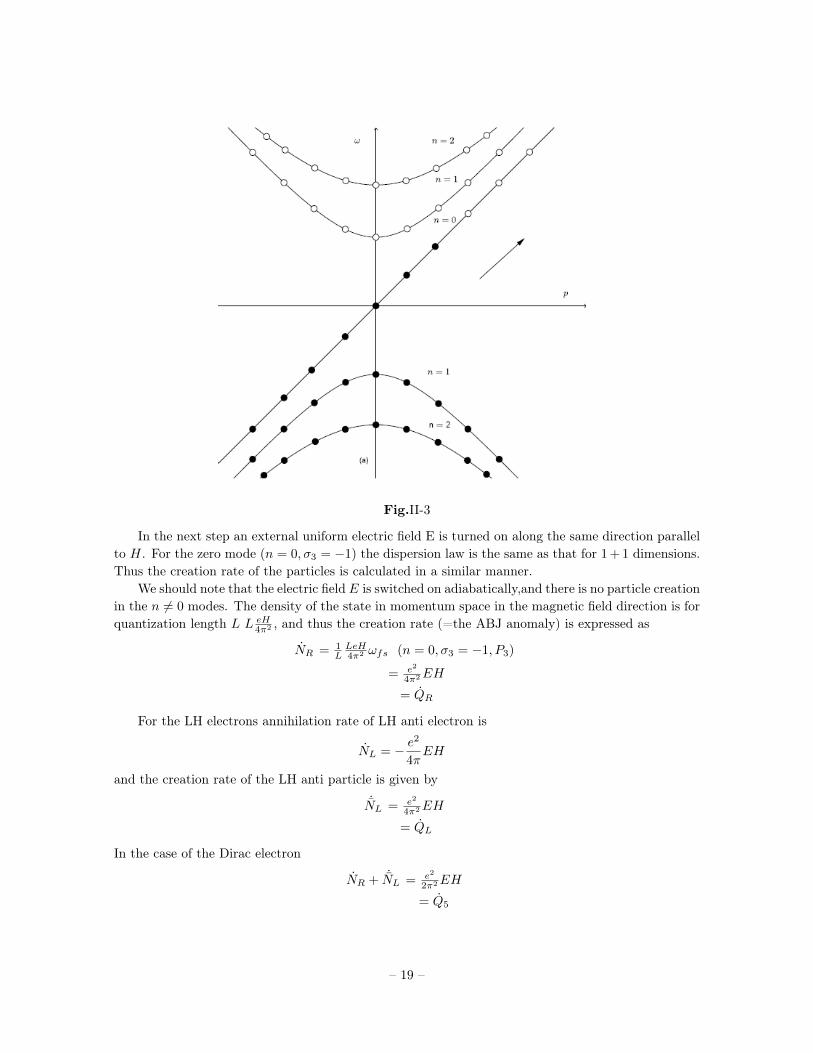
Fig.II-3

In the next step an external uniform electric field E is turned on along the same direction parallelto H. For the zero mode (n = 0, σ3 = −1) the dispersion law is the same as that for 1 + 1 dimensions.Thus the creation rate of the particles is calculated in a similar manner.

We should note that the electric field E is switched on adiabatically,and there is no particle creationin the n 6= 0 modes. The density of the state in momentum space in the magnetic field direction is forquantization length L L eH

4π2 , and thus the creation rate (=the ABJ anomaly) is expressed as

NR = 1LLeH4π2 ωfs (n = 0, σ3 = −1, P3)

= e2

4π2EH

= QR

For the LH electrons annihilation rate of LH anti electron is

NL = − e2

4πEH

and the creation rate of the LH anti particle is given by

˙NL = e2

4π2EH

= QL

In the case of the Dirac electron

NR + ˙NL = e2

2π2EH

= Q5

– 19 –

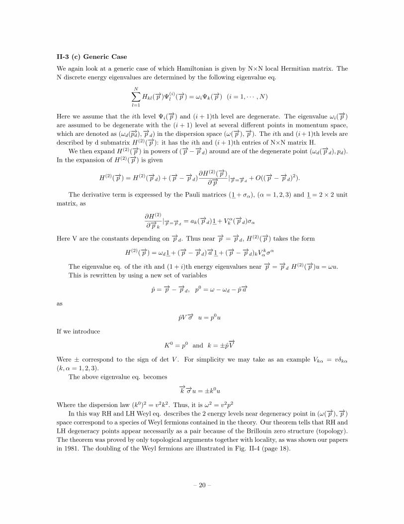
II-3 (c) Generic Case

We again look at a generic case of which Hamiltonian is given by N×N local Hermitian matrix. TheN discrete energy eigenvalues are determined by the following eigenvalue eq.

N∑l=1

Hkl(−→p )Ψ

(i)l (−→p ) = ωiΨk(−→p ) (i = 1, · · · , N)

Here we assume that the ith level Ψi(−→p ) and (i + 1)th level are degenerate. The eigenvalue ωi(−→p )

are assumed to be degenerate with the (i + 1) level at several different points in momentum space,which are denoted as (ωd(−→pd),−→p d) in the dispersion space (ω(−→p ),−→p ). The ith and (i+ 1)th levels aredescribed by d submatrix H(2)(−→p ): it has the ith and (i+ 1)th entries of N×N matrix H.

We then expand H(2)(−→p ) in powers of (−→p −−→p d) around are of the degenerate point (ωd(−→p d), pd).In the expansion of H(2)(−→p ) is given

H(2)(−→p ) = H(2)(−→p d) + (−→p −−→p d)∂H(2)(−→p )

∂−→p|−→p =−→p d +O((−→p −−→p d)2).

The derivative term is expressed by the Pauli matrices (_1 + σα), (α = 1, 2, 3) and _1 = 2× 2 unitmatrix, as

∂H(2)

∂−→p k|−→p =−→p d = ak(−→p d)_1 + V αk (−→p d)σα

Here V are the constants depending on −→p d. Thus near −→p = −→p d, H(2)(−→p ) takes the form

H(2)(−→p ) = ωd_1 + (−→p −−→p d)−→a _1 + (−→p −−→p d)kV kα σα

The eigenvalue eq. of the ith and (1 + i)th energy eigenvalues near −→p = −→p d H(2)(−→p )u = ωu.This is rewritten by using a new set of variables

p = −→p −−→p d, p0 = ω − ωd − p−→a

as

pV−→σ u = p0u

If we introduce

K0 = p0 and k = ±p−→V

Were ± correspond to the sign of det V . For simplicity we may take as an example Vkα = vδkα(k, α = 1, 2, 3).

The above eigenvalue eq. becomes−→k −→σ u = ±k0u

Where the dispersion law (k0)2 = v2k2. Thus, it is ω2 = v2p2

In this way RH and LH Weyl eq. describes the 2 energy levels near degeneracy point in (ω(−→p ),−→p )

space correspond to a species of Weyl fermions contained in the theory. Our theorem tells that RH andLH degeneracy points appear necessarily as a pair because of the Brillouin zero structure (topology).The theorem was proved by only topological arguments together with locality, as was shown our papersin 1981. The doubling of the Weyl fermions are illustrated in Fig. II-4 (page 18).

– 20 –

II-4 Parity non-invariant zero-gap material

We assume that we have found a parity non invariant material (i.e. a crystal should be of non-centrosymmetric symmetry; e.g. BiTeI form a non-centrosymmetric crystal. Best might be a triclinicpedial class with no point symmetry at all.) with zero-gap, which can be simulated by a Weyl,fermion theory with a dispersion law ω2 = v2p2. The effect analogous to the ABJ anomaly gives riseto a peculiar behavior of the conductivity of the electric current in the presence of the magnetic field.It is enough to consider one conduction band ωi.

The valence band ωi+1 (negative energy state) is assumed to be completely filled. In the absenceof external field, the single electron distribution function in the thermodynamical equilibrium is of theform f0(−→p ) = [1 + exp[(ω(p)− u)/kT ]]−1

In the presence of E and H = 0 there occurs a small deviation from thermodynamical equilibriumso that f = f0 + δf , and the E field accelerates the electrons in the same direction and then(

∂f

∂t

)drift

= eE∂f

∂pz.

At the same time the accelerated electrons get scattered back into some states in the same cone. Weassume that f fills back into f0 exponentially with a relaxation time τ0 so that δf ∝ e−

ττ0

Then (∂f

∂t

)coll

= − 1

τ0(f − f0)

Therefore the steady state condition is(∂f∂t

)drift

= −(∂f∂t coll

)(Boltzmann eq.).

The sol. of this is in the lowest order in E

f(−→p ) = f0(ω) + eEτ0∂f(ω)

∂pz

Then the longitudinal current density is given by

J0 =1

L3

∑−→p

(−e)vzf(−→p )(#deg. pts)

Where vz = ∂ω∂pz

and (#deg. pt) denotes the number of deg. pts (= degeneracy points).In the low temperature approximation f0(ω) = θ(µ− ω) so that

J0 =1

6π2e2E(

µ2

v)τ0(#deg. pt)

the relaxation time is given in terms of transition probability of electron from the state with _−→p intoone with _−→p ′, W (−→p → −→p ′) by

1

τ0=

1

L3

∑−→p ′

pz − p′Zpz

W (−→p → −→p ′)

We assume that the interaction between the electron and the ionized impurities is given by the screenedCoulomb potential (pot.) of the from

V (−→x ) =

(4πe2

k

)e−|−→x |γ0

|−→x |

– 21 –

With the screening length γ0 and k the dielectric constant. Computing τ0 in the first order perturbationwe obtain the current as

J0 =4e2E

3πηI

(k

4πe2

)2(µ4

v2

)[ln(1 + β)− β

1 + β

]−1(#deg. pt)

With β = 2πkve2 (#deg. pt) and ηI the density of impurity.

Next compute the magneto-conductivity when H parallel to E is so strong that only the loweststates n = 0, σ3 = −1 with dispersion law ω = vpz or ω = −vpz near the RH and LH degeneracy pointare filled the ABJ anomaly effect will cause the movement in the momentum space of electrons fromthe lowest Landau level (n = 0, σ3 = −1) at the one deg. pt. (=degeneracy point) in the LH coneto the corresponding one (n = 0, σ3 = −1) in the RH cone (at the RH deg.pt.). Thus these movedelectrons will give raise to a deviation from the thermodynamical equilibrium, that can be expressedby the different chemical potentials for the electrons at the RH degeneracy pt., µR and at the LH oneµL. If one had calculated the relaxation time in the approximation where only one degeneracy point ata time was relevant -such as we did above in the H = 0 case–we would have found 1

τ = 0. This comesout of such a calculation due to the energy conservation factor δ(ω − ω′) = 1

v δ(pz − p′z) contained in

W (PZ − P ′Z) which makes (23) give 1τ = 0. However we cannot neglect scattering processes involving

two degeneracy point.

II-5 Transfer from LH to RH cones by Adler-Bell-Jackiw Anomaly

The mechanism for the electric current with both E can H switched on peculiarly different from theone with a negligibly weak H. In the presence of strong H the lattice anomaly of the ABJ anomalytakes place: transfer of the particles from the LH degeneracy pt. to the RH one acts as a drift term,i.e. N |drift in the Boltzmann equation. On the other hand for negligible H each degeneracy points actindependently. By the ABJ anomaly the Fermi energy level µR in the RH cone goes up compared tothat of the H = 0 case µ and µL in the LH cone is lowered. See Fig. II-3 (a) (1 + 1 dim. case) andFig. II-4 (3 + 1 dim. case)

– 22 –

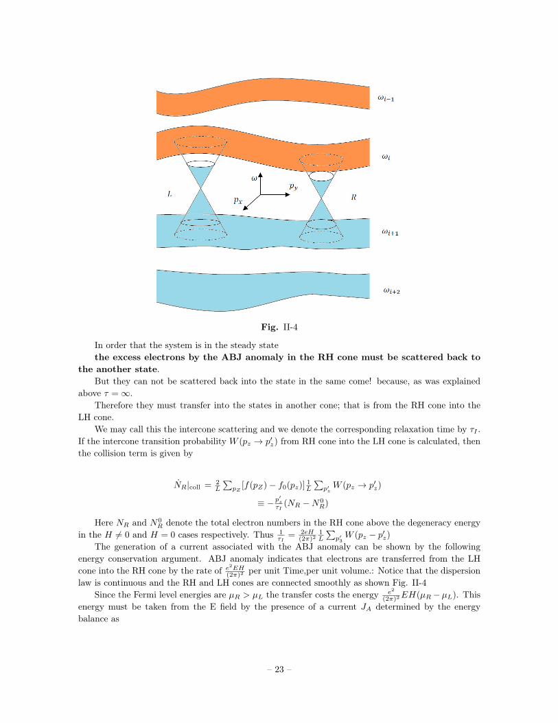
Fig. II-4

In order that the system is in the steady statethe excess electrons by the ABJ anomaly in the RH cone must be scattered back to

the another state.But they can not be scattered back into the state in the same come! because, as was explained

above τ =∞.Therefore they must transfer into the states in another cone; that is from the RH cone into the

LH cone.We may call this the intercone scattering and we denote the corresponding relaxation time by τI .

If the intercone transition probability W (pz → p′z) from RH cone into the LH cone is calculated, thenthe collision term is given by

NR|coll = 2L

∑pZ

[f(pZ)− f0(pz)]1L

∑p′zW (pz → p′z)

≡ −p′z

τI(NR −N0

R)

Here NR and N0R denote the total electron numbers in the RH cone above the degeneracy energy

in the H 6= 0 and H = 0 cases respectively. Thus 1τI

= 2eH(2π)2

1L

∑p′3W (pz − p′z)

The generation of a current associated with the ABJ anomaly can be shown by the followingenergy conservation argument. ABJ anomaly indicates that electrons are transferred from the LHcone into the RH cone by the rate of e

2EH(2π)2 per unit Time,per unit volume.: Notice that the dispersion

law is continuous and the RH and LH cones are connected smoothly as shown Fig. II-4Since the Fermi level energies are µR > µL the transfer costs the energy e2

(2π)2EH(µR−µL). Thisenergy must be taken from the E field by the presence of a current JA determined by the energybalance as

– 23 –

EJA = e2

(2π)2 eH(µR − µL)

At the zero temperature, in the RH conef0(ω) = θ(µR − ω) and thus

NR = 1L3

∑pypz

f0(ω) eH(2π)2

µRv

∼= N0R + (µR − µ)∂NR∂µ

Inserting this into Boltzmann eq.NR|drift = −NR|colWe obtain µR − µL = evEτITherefore JA = ev e2

(2π)2EHτI(#deg.pt.) Here the subscript A stands for the anomalous currentthe one associated with the analogue of the ABJ anomaly. In the definition of τI we may approximateW (−→pz → p′z)

∼= W (−→p −−→p′ )

So that W (pZ − p′Z) ∼= ( 4π2

k )2ηI

[(−→p −−→p ′)2 + 1

γ2H

]−22πδ(ω − ω′) with 1

γ2H

= EHkv (#deg.pt.).

According to −→p ≡ −→p −−→p d, p0 = ω − ωd − p−→a , we have −→p −−→p ′ = −→p d −−→p ′d + −→p − p′

where −→p and −→p′are oscillating around −→p d and −→p ′d: since they are order of (eH)

12 . We may

ignore the oscillatory part (−→p − −→p′) and 1

γ2H

term in the denominator of W (pZ − p′Z) when comparedto the distance of the RH and LH deg. pts −→p d −−→p ′d. In this approximation we obtain

JA = e2v2E2πηI

(k

4π2

)2(−→p d −−→p ′d)4(#deg.pt.)

We then obtain the ratio of the conductivity that is defined by f = σE as σAσ0= 3

16

(vµ

)4 [ln(1 + β)− β

1+β

](−→p d−

−→p ′d)4By these results, for the intercom relation time τI the electrons must travel a “long distance” in

momentum space. Thus τI is expected to be a large value compared to τ0 for H = 0. Therefore σAσ0

given above is large.

II-6 Further arguments

So far we have presented our own theoretical predictions in 1983 although we believed sooner or laterour predicted “Nielsen-Ninomiya” mechanism (or effect) will be proved by experiment. Indeed afteralmost 35 year later Princeton University group led by Prof. N. Phuan Ong and R. Cava, found chiralanomaly in crystalline material. This surprising news in science community appeared in an article byCatherine Zandonella,

• office of the Dean of Research, in Science, September 3, 2015 entitled Research at Princeton:Long-sought chiral anomaly detected in crystalline material (science).

At the almost same time, scientist’s article entitled.

• “Evidence for the chiral anomaly in the Dirac semimetal Na3Bi” By J. Xiong Satya K. Kushwaha,Tian Liang, J. W. Kritzan, M. Hirsehberger, Wulin Wang, R. J. Cava, X. P. Oug, Science Express,03 , September 2015. and

• “Signature of the chiral anomaly in a Dirac semimetal – a current plume steered by J. Xiong, S.K. Kushwaraha, T. Liang, J. W. Krizan, Wudi Wang, R. J. Cava and N. P. Ong

– 24 –

Since then the works on this subject is really under rapidly developing mainly in Experiments,also theories: e. g. Dirac cones,and Weyl semimetals. We believe in the rather near future we shallsee some machines using “Nielsen-Ninomiya Mechanism (or Effect). See e.g also [4].

II-7 Conclusions

In the present article we present the viewpoint at two exceptional high energy theoretical physicistsnew eras of condensed matter.

In the first part I we mainly considered “Topological Insulator” from random dynamics point ofview. The essential point is that in generic Fermion dispersion relations i.e. in (almost) all solids orfluids at low temperature we can derive the recently found properties of Topological insulators suchas graphene etc.

In the 2nd point II, we present what comes beyond topological insulator.We believe that the Adler-Bell-Jackiw anomaly effect in the chiral non invariant gapless material,

causes that

• magnetic conductance is enhanced very much (ideally permanent current)

• Chiral electron (chiral fermion in general) in lattice of the gapless material runs with a fixedspeed. (This fixed speed is what in the relativity theory analogue is the speed of light.) This isso, because we by analogy can apply the relativistic quantum field theory.

To make any apparatus using the above theory will be widely opened to not only condensed matter,but chemistry, beyond artificial division such as, physics chemistry engineering etc.

– 25 –

Acknowledgements

One of the authors (H. B. N.) acknowledges the Niels Bohr Institute, Copenhagen University forallowance to work as emeritus and for economical support to visit the conference in New York forwhich this work is the proceeding. M. N. acknowledges Advanced Mathematical Institute Osaka CityUniversity, and Yukawa Institute for Theoretical Physics, Kyoto University as emeritus.

M. N. also acknowledges the present research is supported by the JSPS Grant in Aid for ScientificResearch No. ISKO 5063.

– 26 –

Appendix A

We consider electron in quantum field theory (Relativistic quantum mechanics.) We present onlynecessary properties in Appendix A

The electron in the relativistic quantum field theory it is usually described as Dirac field Ψ =(ΨL

ΨR

)where ΨL and ΨR are 2 component fields. Now the electron has intrinsic spin

−→S . Thus

electron has the angular momentum then−→J , whose value are half integers, and the spin components

is−→S take values ± 1

2 .For massless fermions the right ΨR and the left ΨL componets in the (free) Dirac equation gets

seperated, and we actually even find that the spin direction is the same as that of electron movementfor the right components ΨR and the opposite for the left components ΨL. Let us start with the Diracfield such as an electron in the quantum field theory. The electron has intrinsic spin 1

2 of fermionobeying the free Dirac eq.

(iγµ∂µ −me)ΨD = 0 (II− 1)

thereafter we ignore electron mass unless described. Our notation is that of the textbook of Bjorken-Drell “ Relativistic Quantum Fields”. For our purpose we list up relevant notations below

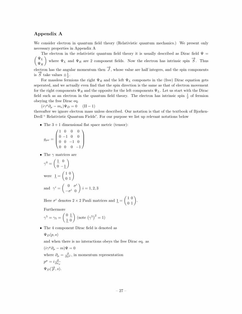
• The 3 + 1 dimensional flat space metric (tensor):

gµν =

1 0 0 0

0 −1 0 0

0 0 −1 0

0 0 0 −1

• The γ matrices are

γ0 =

(_1 0

0 −_1

)were _1 =

(1 0

0 1

)and γi =

(0 σi

−σi 0

)i = 1, 2, 3

Here σi denotes 2× 2 Pauli matrices and _1 =

(1 0

0 1

).

Furthermore

γ5 = γ5 =

(0 _1_1 0

)(note

(γ5)2

= 1)

• The 4 component Dirac field is denoted as

ΨD(p, s)

and when there is no interactions obeys the free Dirac eq. as

(iγµ∂µ −m)Ψ = 0

where ∂µ = ∂∂xµ , in momentum representation

pµ = i ∂∂xµ

ΨD(−→p , s).

– 27 –

Here s denote intrinsic spin |s| = 12

ΨD(−→p ,−→s ) obeys

/pΨD(p, s) = 0

with 4 component Dirac field we may describe

ΨD(p, s) =

(ΨL

ΨR

)(p, s)

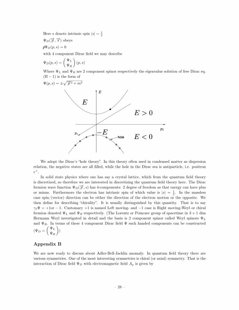
Where ΨL and ΨR are 2 component spinor respectively the eigenvalue solution of free Dirac eq.(II− 1) is the form of

Ψ(p, s) = ±√−→p 2 +m2

We adopt the Dirac’s “hole theory”. In this theory often used in condensed matter as dispersionrelation, the negative states are all filled, while the hole in the Dirac sea is antiparticle, i.e. positrone+.

In solid state physics where one has say a crystal lattice, which from the quantum field theoryis discretized, so therefore we are interested in discretizing the quantum field theory here. The Diracfermion wave function ΨD(−→p , s) has 4-components: 2 degree of freedom as that energy can have plusor minus. Furthermore the electron has intrinsic spin of which value is |s| = 1

2 . In the masslesscase spin/(vector) direction can be either the direction of the electron motion or the opposite. Wethen define for describing “chirality”. It is usually distinguished by this quantity. That is to sayγ5Ψ = +1or − 1. Customary +1 is named Left moving- and −1 case is Right moving-Weyl or chiralfermion denoted ΨL and ΨR respectively. (The Lorentz or Poincare group of spacetime in 3 + 1 dimHermann Weyl investigated in detail and the basis is 2 component spinor called Weyl spinors ΨL

and ΨR. In terms of these 4 component Dirac field Ψ such handed components can be constructed

(ΨD =

(ΨL

ΨR

))

Appendix B

We are now ready to discuss about Adler-Bell-Jacklin anomaly. In quantum field theory there arevarious symmetries. One of the most interesting symmetries is chiral (or axial) symmetry. That is theinteraction of Dirac field ΨD with electromagnetic field Aµ is given by

– 28 –

S =∫d4xΨ(x) [iγµ (∂µ + ieAµ(x))] ΨD(x) (∗)

in the case of massless electron., where ΨD = Ψ†γ0. It has chiral symmetry which may be obvious, ifwe rewrite (∗) in terms of ΨL and ΨR as the Dirac eq. can be written as(

0 i(∂0 + σi(∂i + ieAi))

i(∂0 − σi(∂i + ieAi)) 0

)(ΨL

ΨR

)= 0.

In this way the equations of ΨL and ΨR are separately given by the following Weyl equations

i(∂0 − σi(∂i +Ai))ΨL = 0

andi(∂0 + σi(∂i +Ai))ΨR = 0.

In these forms it is evident that the theories are invariant under the following infinitesimal Weyltransformations

ΨL → (1− iαi σi2 − βi σi2 )ΨL

ΨR → (1− iαi σi2 + βi σi2 )ΨR

Where αi and βi (i = 1, 2, 3) are infinitesimal transformation parameters, restricted to leave thenormalization of the Weyl fields invariant. This Weyl or Chiral transformation is broken due to quan-tum effect in quantum field theory. There were several suggestive articles, but explicit manifestationis presented by

• S. Adler, Phys. Rev. 177 (1969) 2426

and

• J. S. Bell and R. Jackiw Nuovo Cimento 60A (1969) 4.

Furthermore the method of path integral formulation this ABJ anomaly is due to nor-invariance ofthe path integral measure

• K. Fujikawa Phys. Rev. Lett. 42 1195 (1979)

Phenomenologically this ABJ anomaly is really important. It has been observed by experiments. Π0

meson decays into 2 photons. When we approximate Π0 as being massless, this decay process isexpressed as the following diagram, triangle diagram of Feynman diagram

– 29 –

If chiral symmetry is not broken, this diagram turns out to give zero. Thus this decay is not al-lowed. However, experimentally this decay process certainly exists. This is the evidence that Adler-Bell-Jackiw anomaly does exist. In high energy, physics the ABJ anomaly is expressed as the non-conservation chiral current J5

µ such that∂µJ5

µ = − e2

16π2 εαβγδFαβFγδ

Here the chiral current J5µ is defined as

J5µ = limε→0

{Ψ(x+ ε

2 )γµγ5exp

[−ie

∫ x+ ε2

x− ε2dzA(z)

]Ψ(x+ ε

2 )}

We might perform the calculation to show that the above triangle diagram is non-zero due to theABJ anomaly. But we have instead in subsection alluded to a derivation of the ABJ-anomaly byusing how particles are pumped up or down from or to the fermi-sea (in high energy physics the Diracsea).

References

[1] Jahn, H. A.; Teller, E. (1937). "Stability of polyatomic molecules in degenerate electronic states. I.Orbital degeneracy". Proc. R. Soc. A. 161 (A905): 220âĂŞ235. Bibcode:1937RSPSA.161..220J.doi:10.1098/rspa.1937.0142.

[2] Kramers, H. A., Proc. Amsterdam Acad. 33, 959 (1930) E. Wigner, Über die Operation der Zeitumkehrin der Quantenmechanik, Nachr. Akad. Ges. Wiss. Göttingen 31, 546âĂŞ559 (1932)http://www.digizeitschriften.de/dms/img/?PPN=GDZPPN002509032

[3] Nuclear Physics B - Proceedings Supplements Volume 29, Issues 2âĂŞ3, December 1992, Pages 200-246“Weyl particles, weak interactions & origin of geometry” https://doi.org/10.1016/0920-5632(92)90021-J

[4] Qiang Li, Dmitri E.Kharzeev, Nuclear Physics A Volume 956, December 2016, Pages 107-111 “Chiralmagnetic effect in condensed matter systems”

– 30 –