arX

iv:1

005.

0252

v1 [

mat

h.O

C]

3 M

ay 2

010

Discrete-Time Fractional Variational Problems

Nuno R. O. Bastosa, Rui A. C. Ferreirab, Delfim F. M. Torresc

aDepartment of Mathematics, ESTGVPolytechnic Institute of Viseu3504-510 Viseu, Portugal

bFaculty of Engineering and Natural SciencesLusophone University of Humanities and Technologies

1749-024 Lisbon, PortugalcDepartment of Mathematics

University of Aveiro3810-193 Aveiro, Portugal

Abstract

We introduce a discrete-time fractional calculus of variations on the time scalehZ, h > 0. First and second order necessary optimality conditions are estab-lished. Examples illustrating the use of the new Euler-Lagrange and Legendretype conditions are given. They show that solutions to the considered frac-tional problems become the classical discrete-time solutions when the fractionalorder of the discrete-derivatives are integer values, and that they converge to thefractional continuous-time solutions when h tends to zero. Our Legendre typecondition is useful to eliminate false candidates identified via the Euler-Lagrangefractional equation.

Keywords: Fractional difference calculus, calculus of variations, fractionalsummation by parts, Euler-Lagrange equation, natural boundary conditions,Legendre necessary condition, time scale hZ.2010 MSC: 26A33, 39A12, 49K05.

1. Introduction

The Fractional Calculus (calculus with derivatives of arbitrary order) is animportant research field in several different areas such as physics (includingclassical and quantum mechanics as well as thermodynamics), chemistry, biol-ogy, economics, and control theory [3, 10, 40, 42, 48]. It has its origin morethan 300 years ago when L’Hopital asked Leibniz what should be the meaningof a derivative of non-integer order. After that episode several more famousmathematicians contributed to the development of Fractional Calculus: Abel,Fourier, Liouville, Riemann, Riesz, just to mention a few names [30, 47]. In thelast decades, considerable research has been done in fractional calculus. This isparticularly true in the area of the calculus of variations, which is being subject

Email addresses: nbastos@estv.ipv.pt (Nuno R. O. Bastos), ruiacferreira@ua.pt(Rui A. C. Ferreira), delfim@ua.pt (Delfim F. M. Torres)

Submitted 24/Nov/2009; Revised 16/Mar/2010; Accepted 3/May/2010; for publication in Signal Processing.

to intense investigations during the last few years [10, 11, 44, 45]. Applica-tions include fractional variational principles in mechanics and physics, quan-tization, control theory, and description of conservative, nonconservative, andconstrained systems [10, 15, 16, 45]. Roughly speaking, the classical calculus ofvariations and optimal control is extended by substituting the usual derivativesof integer order by different kinds of fractional (non-integer) derivatives. It isimportant to note that the passage from the integer/classical differential calcu-lus to the fractional one is not unique because we have at our disposal differentnotions of fractional derivatives. This is, as argued in [10, 44], an interestingand advantage feature of the area. Most part of investigations in the fractionalvariational calculus are based on the replacement of the classical derivativesby fractional derivatives in the sense of Riemann–Liouville, Caputo, Riesz, andJumarie [1, 4, 10, 27]. Independently of the chosen fractional derivatives, oneobtains, when the fractional order of differentiation tends to an integer order,the usual problems and results of the calculus of variations. Although the frac-tional Euler–Lagrange equations are obtained in a similar manner as in thestandard variational calculus [44], some classical results are extremely difficultto be proved in a fractional context. This explains, for example, why a fractionalLegendre type condition is absent from the literature of fractional variationalcalculus. In this work we give a first result in this direction (cf. Theorem 3.6).

Despite its importance in applications, less is known for discrete-time frac-tional systems [44]. In [39] Miller and Ross define a fractional sum of orderν > 0 via the solution of a linear difference equation. They introduce it as (see§2 for the notations used here)

∆−νf(t) =1

Γ(ν)

t−ν∑

s=a

(t− σ(s))(ν−1)f(s). (1)

Definition (1) is analogous to the Riemann-Liouville fractional integral

aD−νx f(x) =

1

Γ(ν)

∫ x

a

(x− s)ν−1f(s)ds

of order ν > 0, which can be obtained via the solution of a linear differentialequation [39, 40]. Basic properties of the operator ∆−ν in (1) were obtainedin [39]. More recently, Atici and Eloe introduced the fractional difference oforder α > 0 by ∆αf(t) = ∆m(∆α−mf(t)), where m is the integer part of α,and developed some of its properties that allow to obtain solutions of certainfractional difference equations [8, 9].

The fractional differential calculus has been widely developed in the past fewdecades due mainly to its demonstrated applications in various fields of scienceand engineering [30, 40, 43]. The study of necessary optimality conditions forfractional problems of the calculus of variations and optimal control is a fairlyrecent issue attracting an increasing attention – see [1, 2, 7, 22, 23, 25, 26, 41]and references therein – but available results address only the continuous-timecase. It is well known that discrete analogues of differential equations can bevery useful in applications [13, 31, 29] and that fractional Euler-Lagrange dif-ferential equations are extremely difficult to solve, being necessary to discretizethem [2, 11]. Therefore, it is pertinent to develop a fractional discrete-timetheory of the calculus of variations for the time scale (hZ)a, h > 0 (cf. defini-

2

tions in Section 2). Computer simulations show that this time scale is particu-larly interesting because when h tends to zero one recovers previous fractionalcontinuous-time results.

Our objective is two-fold. On one hand we proceed to develop the theory offractional difference calculus, namely, we introduce the concept of left and rightfractional sum/difference (cf. Definition 2.8). On the other hand, we believethat the present work will potentiate research not only in the fractional calculusof variations but also in solving fractional difference equations, specifically, frac-tional equations in which left and right fractional differences appear. Becausethe theory of fractional difference calculus is still in its infancy [8, 9, 39], thepaper is self contained. In §2 we introduce notations, we give necessary defini-tions, and prove some preliminary results needed in the sequel. Main results ofthe paper appear in §3: we prove a fractional formula of h-summation by parts(Theorem 3.2), and necessary optimality conditions of first and second order(Theorems 3.5 and 3.6, respectively) for the proposed h-fractional problem ofthe calculus of variations (17). Section 4 gives some illustrative examples, andwe end the paper with §5 of conclusions and future perspectives.

The results of the paper are formulated using standard notations of thetheory of time scales [20, 32, 33]. It remains an interesting open question how togeneralize the present results to an arbitrary time scale T. This is a difficult andchallenging problem since our proofs deeply rely on the fact that in T = (hZ)athe graininess function is a constant.

2. Preliminaries

We begin by recalling the main definitions and properties of time scales(cf. [18, 20] and references therein). A nonempty closed subset of R is calleda time scale and is denoted by T. The forward jump operator σ : T → T isdefined by σ(t) = inf {s ∈ T : s > t} for all t ∈ T, while the backward jumpoperator ρ : T → T is defined by ρ(t) = sup {s ∈ T : s < t} for all t ∈ T, withinf ∅ = supT (i.e., σ(M) = M if T has a maximum M) and sup ∅ = inf T(i.e., ρ(m) = m if T has a minimum m). A point t ∈ T is called right-dense,right-scattered, left-dense, or left-scattered, if σ(t) = t, σ(t) > t, ρ(t) = t, orρ(t) < t, respectively. Throughout the text we let T = [a, b] ∩ T with a < b and

T a time scale. We define Tκ = T\(ρ(b), b], Tκ2

= (Tκ)κand more generally

Tκn

=(

Tκn−1

)κ

, for n ∈ N. The following standard notation is used for σ

(and ρ): σ0(t) = t, σn(t) = (σ ◦ σn−1)(t), n ∈ N. The graininess functionµ : T → [0,∞) is defined by µ(t) = σ(t) − t for all t ∈ T.

A function f : T → R is said to be delta differentiable at t ∈ Tκ if there is

a number f∆(t) such that for all ε > 0 there exists a neighborhood U of t (i.e.,U = (t− δ, t+ δ) ∩ T for some δ > 0) such that

|f(σ(t))− f(s)− f∆(t)(σ(t) − s)| ≤ ε|σ(t) − s|, for all s ∈ U.

We call f∆(t) the delta derivative of f at t. The rth−delta derivative (r ∈ N)

of f is defined to be the function f∆r

: Tκr

→ R, provided f∆r−1

is deltadifferentiable on T

κr−1

. For delta differentiable f and g and for an arbitrarytime scale T the next formulas hold: fσ(t) = f(t) + µ(t)f∆(t) and

(fg)∆(t) = f∆(t)gσ(t) + f(t)g∆(t) = f∆(t)g(t) + fσ(t)g∆(t), (2)

3

where we abbreviate f ◦ σ by fσ. A function f : T → R is called rd-continuousif it is continuous at right-dense points and if its left-sided limit exists at left-dense points. The set of all rd-continuous functions is denoted by Crd and theset of all delta differentiable functions with rd-continuous derivative by C1

rd.It is known that rd-continuous functions possess an antiderivative, i.e., thereexists a function F ∈ C1

rd with F∆ = f . The delta integral is then defined by∫ b

af(t)∆t = F (b)− F (a). It satisfies the equality

∫ σ(t)

tf(τ)∆τ = µ(t)f(t). We

make use of the following properties of the delta integral:

Lemma 2.1. (cf. [20, Theorem 1.77]) If a, b ∈ T and f, g ∈Crd, then

1.∫ b

af(σ(t))g∆(t)∆t = (fg)(t)|t=b

t=a −∫ b

af∆(t)g(t)∆t;

2.∫ b

a f(t)g∆(t)∆t = (fg)(t)|t=bt=a −

∫ b

a f∆(t)g(σ(t))∆t.

One way to approach the Riemann-Liouville fractional calculus is throughthe theory of linear differential equations [43]. Miller and Ross [39] use ananalogous methodology to introduce fractional discrete operators for the caseT = Za = {a, a + 1, a + 2, . . .}, a ∈ R. Here we go a step further: we use thetheory of time scales in order to introduce fractional discrete operators to themore general case T = (hZ)a = {a, a+ h, a+ 2h, . . .}, a ∈ R, h > 0.

For n ∈ N0 and rd-continuous functions pi : T → R, 1 ≤ i ≤ n, let usconsider the nth order linear dynamic equation

Ly = 0 , where Ly = y∆n

+

n∑

i=1

piy∆n−i

. (3)

A function y : T → R is said to be a solution of equation (3) on T provided y isn times delta differentiable on T

κn

and satisfies Ly(t) = 0 for all t ∈ Tκn

.

Lemma 2.2. [20, p. 239] If z = (z1, . . . , zn) : T → Rn satisfies for all t ∈ T

κ

z∆ = A(t)z(t), where A =

0 1 0 . . . 0... 0 1

. . ....

.... . .

. . . 00 . . . . . . 0 1

−pn . . . . . . −p2 −p1

(4)

then y = z1 is a solution of equation (3). Conversely, if y solves (3) on T, then

z =(

y, y∆, . . . , y∆n−1)

: T → R satisfies (4) for all t ∈ Tκn

Definition 2.3. [20, p. 239] We say that equation (3) is regressive providedI + µ(t)A(t) is invertible for all t ∈ T

κ, where A is the matrix in (4).

Definition 2.4. [20, p. 250] We define the Cauchy function y : T × Tκn

→ R

for the linear dynamic equation (3) to be, for each fixed s ∈ Tκn

, the solutionof the initial value problem

Ly = 0, y∆i

((σ(s), s) = 0, 0 ≤ i ≤ n− 2, y∆n−1

((σ(s), s) = 1 . (5)

4

Theorem 2.5. [20, p. 251] Suppose {y1, . . . , yn} is a fundamental system ofthe regressive equation (3). Let f ∈ Crd. Then the solution of the initial valueproblem

Ly = f(t), y∆i

(t0) = 0, 0 ≤ i ≤ n− 1 ,

is given by y(t) =∫ t

t0y(t, s)f(s)∆s, where y(t, s) is the Cauchy function for (3).

It is known that y(t, s) := Hn−1(t, σ(s)) is the Cauchy function for y∆n

= 0,where Hn−1 is a time scale generalized polynomial [20, Example 5.115]. Thegeneralized polynomials Hk are the functions Hk : T2 → R, k ∈ N0, definedrecursively as follows:

H0(t, s) ≡ 1 , Hk+1(t, s) =

∫ t

s

Hk(τ, s)∆τ , k = 1, 2, . . .

for all s, t ∈ T. If we let H∆k (t, s) denote, for each fixed s, the derivative of

Hk(t, s) with respect to t, then (cf. [20, p. 38])

H∆k (t, s) = Hk−1(t, s) for k ∈ N, t ∈ T

κ .

From now on we restrict ourselves to the time scale T = (hZ)a, h > 0, forwhich the graininess function is the constant h. Our main goal is to propose anddevelop a discrete-time fractional variational theory in T = (hZ)a. We borrowthe notations from the recent calculus of variations on time scales [18, 24, 32].How to generalize our results to an arbitrary time scale T, with the graininessfunction µ depending on time, is not clear and remains a challenging question.

Let a ∈ R and h > 0, (hZ)a = {a, a+h, a+2h, . . .}, and b = a+kh for somek ∈ N. We have σ(t) = t + h, ρ(t) = t − h, µ(t) ≡ h, and we will frequentlywrite fσ(t) = f(σ(t)). We put T = [a, b] ∩ (hZ)a, so that Tκ = [a, ρ(b)] ∩ (hZ)aand T

κ2

= [a, ρ2(b)] ∩ (hZ)a. The delta derivative coincides in this case with

the forward h-difference: f∆(t) =fσ(t)− f(t)

µ(t). If h = 1, then we have the

usual discrete forward difference ∆f(t). The delta integral gives the h-sum

(or h-integral) of f :

∫ b

a

f(t)∆t =

bh−1∑

k= ah

f(kh)h. If we have a function f of two

variables, f(t, s), its partial forward h-differences will be denoted by ∆t,h and

∆s,h, respectively. We will make use of the standard conventions∑c−1

t=c f(t) =

0, c ∈ Z, and∏−1

i=0 f(i) = 1. Often, left fractional delta integration (resp.,right fractional delta integration) of order ν > 0 is denoted by a∆

−νt f(t) (resp.

t∆−νb f(t)). Here, similarly as in Ross et. al. [46], where the authors omit the

subscript t on the operator (the operator itself cannot depend on t), we write

a∆−νh f(t) (resp. h∆

−νb f(t)).

Before giving an explicit formula for the generalized polynomials Hk on hZwe introduce the following definition:

Definition 2.6. For arbitrary x, y ∈ R the h-factorial function is defined by

x(y)h := hy Γ(xh + 1)

Γ(xh + 1− y),

where Γ is the well-known Euler gamma function, and we use the conventionthat division at a pole yields zero.

5

Remark 2.1. For h = 1, and in accordance with the previous literature (1), we

write x(y) to denote x(y)h .

Proposition 2.1. For the time-scale T = (hZ)a one has

Hk(t, s) :=(t− s)

(k)h

k!for all s, t ∈ T and k ∈ N0 . (6)

To prove (6) we use the following technical lemma. Throughout the text thebasic property Γ(x+1) = xΓ(x) of the gamma function will be frequently used.

Lemma 2.7. Let s ∈ T. Then, for all t ∈ Tκ one has

∆t,h

{

(t− s)(k+1)h

(k + 1)!

}

=(t− s)

(k)h

k!.

Proof. The equality follows by direct computations:

∆t,h

{

(t− s)(k+1)h

(k + 1)!

}

=1

h

{

(σ(t) − s)(k+1)h

(k + 1)!−

(t− s)(k+1)h

(k + 1)!

}

=hk+1

h(k + 1)!

{Γ((t+ h− s)/h+ 1)

Γ((t+ h− s)/h+ 1− (k + 1))−

Γ((t− s)/h+ 1)

Γ((t− s)/h+ 1− (k + 1))

}

=hk

(k + 1)!

{((t− s)/h+ 1)Γ((t− s)/h+ 1)

((t− s)/h− k)Γ((t− s)/h− k)−

Γ((t− s)/h+ 1)

Γ((t− s)/h− k)

}

=hk

k!

{Γ((t− s)/h+ 1)

Γ((t− s)/h+ 1− k)

}

=(t− s)

(k)h

k!.

Proof. (of Proposition 2.1) We proceed by mathematical induction. For k = 0

H0(t, s) =1

0!h0 Γ( t−s

h + 1)

Γ( t−sh + 1− 0)

=Γ( t−s

h + 1)

Γ( t−sh + 1)

= 1 .

Assume that (6) holds for k replaced by m. Then by Lemma 2.7

Hm+1(t, s) =

∫ t

s

Hm(τ, s)∆τ =

∫ t

s

(τ − s)(m)h

m!∆τ =

(t− s)(m+1)h

(m+ 1)!,

which is (6) with k replaced by m+ 1.

Let y1(t), . . . , yn(t) be n linearly independent solutions of the linear homoge-neous dynamic equation y∆

n

= 0. From Theorem 2.5 we know that the solutionof (5) (with L = ∆n and t0 = a) is

y(t) = ∆−nf(t) =

∫ t

a

(t− σ(s))(n−1)h

Γ(n)f(s)∆s =

1

Γ(n)

t/h−1∑

k=a/h

(t−σ(kh))(n−1)h f(kh)h .

6

Since y∆i(a) = 0, i = 0, . . . , n− 1, then we can write that

∆−nf(t) =1

Γ(n)

t/h−n∑

k=a/h

(t− σ(kh))(n−1)h f(kh)h

=1

Γ(n)

∫ σ(t−nh)

a

(t− σ(s))(n−1)h f(s)∆s .

(7)

Note that function t → (∆−nf)(t) is defined for t = a + nh mod(h) whilefunction t → f(t) is defined for t = a mod(h). Extending (7) to any positivereal value ν, and having as an analogy the continuous left and right fractionalderivatives [40], we define the left fractional h-sum and the right fractional h-sum as follows. We denote by FT the set of all real valued functions defined ona given time scale T.

Definition 2.8. Let a ∈ R, h > 0, b = a + kh with k ∈ N, and put T =[a, b] ∩ (hZ)a. Consider f ∈ FT. The left and right fractional h-sum of orderν > 0 are, respectively, the operators a∆

−νh : FT → F

T+νand h∆

−νb : FT → F

T−

ν,

T±ν = {t± νh : t ∈ T}, defined by

a∆−νh f(t) =

1

Γ(ν)

∫ σ(t−νh)

a

(t− σ(s))(ν−1)h f(s)∆s =

1

Γ(ν)

th−ν∑

k= ah

(t− σ(kh))(ν−1)h f(kh)h

h∆−νb f(t) =

1

Γ(ν)

∫ σ(b)

t+νh

(s− σ(t))(ν−1)h f(s)∆s =

1

Γ(ν)

bh∑

k= th+ν

(kh− σ(t))(ν−1)h f(kh)h.

Remark 2.2. In Definition 2.8 we are using summations with limits that arereals. For example, the summation that appears in the definition of operator

a∆−νh has the following meaning:

th−ν∑

k= ah

G(k) = G(a/h) +G(a/h+ 1) +G(a/h+ 2) + · · ·+G(t/h− ν),

where t ∈ {a+ νh, a+ h+ νh, a+ 2h+ νh, . . . , a+ kh︸ ︷︷ ︸

b

+νh} with k ∈ N.

Lemma 2.9. Let ν > 0 be an arbitrary positive real number. For any t ∈ T wehave: (i) limν→0 a∆

−νh f(t+ νh) = f(t); (ii) limν→0 h∆

−νb f(t− νh) = f(t).

Proof. Since

a∆−νh f(t+ νh) =

1

Γ(ν)

∫ σ(t)

a

(t+ νh− σ(s))(ν−1)h f(s)∆s

=1

Γ(ν)

th∑

k= ah

(t+ νh− σ(kh))(ν−1)h f(kh)h

= hνf(t) +ν

Γ(ν + 1)

ρ(t)h∑

k= ah

(t+ νh− σ(kh))(ν−1)h f(kh)h ,

it follows that limν→0 a∆−νh f(t+ νh) = f(t). The proof of (ii) is similar.

7

For any t ∈ T and for any ν ≥ 0 we define a∆0hf(t) := h∆

0bf(t) := f(t) and

write

a∆−νh f(t+ νh) = hνf(t) +

ν

Γ(ν + 1)

∫ t

a

(t+ νh− σ(s))(ν−1)h f(s)∆s ,

h∆−νb f(t) = hνf(t− νh) +

ν

Γ(ν + 1)

∫ σ(b)

σ(t)

(s+ νh− σ(t))(ν−1)h f(s)∆s .

(8)

Theorem 2.10. Let f ∈ FT and ν ≥ 0. For all t ∈ Tκ we have

a∆−νh f∆(t+ νh) = (a∆

−νh f(t+ νh))∆ −

ν

Γ(ν + 1)(t+ νh− a)

(ν−1)h f(a) . (9)

To prove Theorem 2.10 we make use of a technical lemma:

Lemma 2.11. Let t ∈ Tκ. The following equality holds for all s ∈ T

κ:

∆s,h

(

(t+ νh− s)(ν−1)h f(s))

)

= (t+ νh− σ(s))(ν−1)h f∆(s)− (v − 1)(t+ νh− σ(s))

(ν−2)h f(s) . (10)

Proof. Direct calculations give the intended result:

∆s,h

(

(t+ νh− s)(ν−1)h f(s)

)

= ∆s,h

(

(t+ νh− s)(ν−1)h

)

f(s) + (t+ νh− σ(s))(ν−1)h f∆(s)

=f(s)

h

hν−1Γ(

t+νh−σ(s)h + 1

)

Γ(

t+νh−σ(s)h + 1− (ν − 1)

) − hν−1 Γ(t+νh−s

h + 1)

Γ(t+νh−s

h + 1− (ν − 1))

+ (t+ νh− σ(s))(ν−1)h f∆(s)

= f(s)

[

hν−2

[

Γ( t+νh−sh )

Γ( t−sh + 1)

−Γ( t+νh−s

h + 1)

Γ( t−sh + 2)

]]

+ (t+ νh− σ(s))(ν−1)h f∆(s)

= f(s)hν−2 Γ( t+νh−s−hh + 1)

Γ( t−s+νh−hh + 1− (ν − 2))

(−(ν − 1)) + (t+ νh− σ(s))(ν−1)h f∆(s)

= −(ν − 1)(t+ νh− σ(s))(ν−2)h f(s) + (t+ νh− σ(s))

(ν−1)h f∆(s) ,

where the first equality follows directly from (2).

Remark 2.3. Given an arbitrary t ∈ Tκ it is easy to prove, in a similar way

as in the proof of Lemma 2.11, the following equality analogous to (10): for alls ∈ T

κ

∆s,h

(

(s+ νh− σ(t))(ν−1)h f(s))

)

= (ν − 1)(s+ νh− σ(t))(ν−2)h fσ(s) + (s+ νh− σ(t))

(ν−1)h f∆(s) . (11)

8

Proof. (of Theorem 2.10) From Lemma 2.11 we obtain that

a∆−νh f∆(t+ νh) = hνf∆(t) +

ν

Γ(ν + 1)

∫ t

a

(t+ νh− σ(s))(ν−1)h f∆(s)∆s

= hνf∆(t) +ν

Γ(ν + 1)

[

(t+ νh− s)(ν−1)h f(s)

]s=t

s=a

+ν

Γ(ν + 1)

∫ σ(t)

a

(ν − 1)(t+ νh− σ(s))(ν−2)h f(s)∆s

= −ν(t+ νh− a)

(ν−1)h

Γ(ν + 1)f(a) + hνf∆(t) + νhν−1f(t)

+ν

Γ(ν + 1)

∫ t

a

(ν − 1)(t+ νh− σ(s))(ν−2)h f(s)∆s.

(12)

We now show that (a∆−νh f(t+ νh))∆ equals (12):

(a∆−νh f(t+ νh))∆ =

1

h

[

hνf(σ(t)) +ν

Γ(ν + 1)

∫ σ(t)

a

(σ(t) + νh− σ(s))(ν−1)h f(s)∆s

−hνf(t)−ν

Γ(ν + 1)

∫ t

a

(t+ νh− σ(s))(ν−1)h f(s)∆s

]

= hνf∆(t) +ν

hΓ(ν + 1)

[∫ t

a

(σ(t) + νh− σ(s))(ν−1)h f(s)∆s

−

∫ t

a

(t+ νh− σ(s))(ν−1)h f(s)∆s

]

+ hν−1νf(t)

= hνf∆(t) +ν

Γ(ν + 1)

∫ t

a

∆t,h

(

(t+ νh− σ(s))(ν−1)h

)

f(s)∆s+ hν−1νf(t)

= hνf∆(t) +ν

Γ(ν + 1)

∫ t

a

(ν − 1)(t+ νh− σ(s))(ν−2)h f(s)∆s+ νhν−1f(t) .

Follows the counterpart of Theorem 2.10 for the right fractional h-sum:

Theorem 2.12. Let f ∈ FT and ν ≥ 0. For all t ∈ Tκ we have

h∆−νρ(b)f

∆(t−νh) =ν

Γ(ν + 1)(b+νh−σ(t))

(ν−1)h f(b)+(h∆

−νb f(t−νh))∆ . (13)

Proof. From (11) we obtain from integration by parts (item 2 of Lemma 2.1)that

h∆−νρ(b)f

∆(t− νh) =ν(b + νh− σ(t))

(ν−1)h

Γ(ν + 1)f(b) + hνf∆(t)− νhν−1f(σ(t))

−ν

Γ(ν + 1)

∫ b

σ(t)

(ν − 1)(s+ νh− σ(t))(ν−2)h fσ(s)∆s.

(14)

9

We show that (h∆−νb f(t− νh))∆ equals (14):

(h∆−νb f(t− νh))∆

= hνf∆(t) +ν

hΓ(ν + 1)

[∫ σ(b)

σ2(t)

(s+ νh− σ2(t)))(ν−1)h f(s)∆s

−

∫ σ(b)

σ2(t)

(s+ νh− σ(t))(ν−1)h f(s)∆s

]

− νhν−1f(σ(t))

= hνf∆(t) +ν

Γ(ν + 1)

∫ σ(b)

σ2(t)

∆t,h

(

(s+ νh− σ(t))(ν−1)h

)

f(s)∆s− νhν−1f(σ(t))

= hνf∆(t)−ν

Γ(ν + 1)

∫ σ(b)

σ2(t)

(ν − 1)(s+ νh− σ2(t))(ν−2)h f(s)∆s− νhν−1f(σ(t))

= hνf∆(t)−ν

Γ(ν + 1)

∫ b

σ(t)

(ν − 1)(s+ νh− σ(t))(ν−2)h f(s)∆s− νhν−1f(σ(t)).

Definition 2.13. Let 0 < α ≤ 1 and set γ := 1 − α. The left fractionaldifference a∆

αhf(t) and the right fractional difference h∆

αb f(t) of order α of a

function f ∈ FT are defined as

a∆αhf(t) := (a∆

−γh f(t+ γh))∆ and h∆

αb f(t) := −(h∆

−γb f(t− γh))∆

for all t ∈ Tκ.

3. Main Results

Our aim is to introduce the h-fractional problem of the calculus of variationsand to prove corresponding necessary optimality conditions. In order to obtainan Euler-Lagrange type equation (cf. Theorem 3.5) we first prove a fractionalformula of h-summation by parts.

3.1. Fractional h-summation by parts

A big challenge was to discover a fractional h-summation by parts formulawithin the time scale setting. Indeed, there is no clue of what such a formulashould be. We found it eventually, making use of the following lemma.

Lemma 3.1. Let f and k be two functions defined on Tκ and T

κ2

, respectively,and g a function defined on T

κ × Tκ2

. The following equality holds:

∫ b

a

f(t)

[∫ t

a

g(t, s)k(s)∆s

]

∆t =

∫ ρ(b)

a

k(t)

[∫ b

σ(t)

g(s, t)f(s)∆s

]

∆t .

Proof. Consider the matrices R = [f(a+ h), f(a+ 2h), · · · , f(b− h)],

C1 =

g(a+ h, a)k(a)g(a+ 2h, a)k(a) + g(a+ 2h, a+ h)k(a+ h)

...g(b− h, a)k(a) + g(b− h, a+ h)k(a+ h) + · · ·+ g(b− h, b− 2h)k(b− 2h)

10

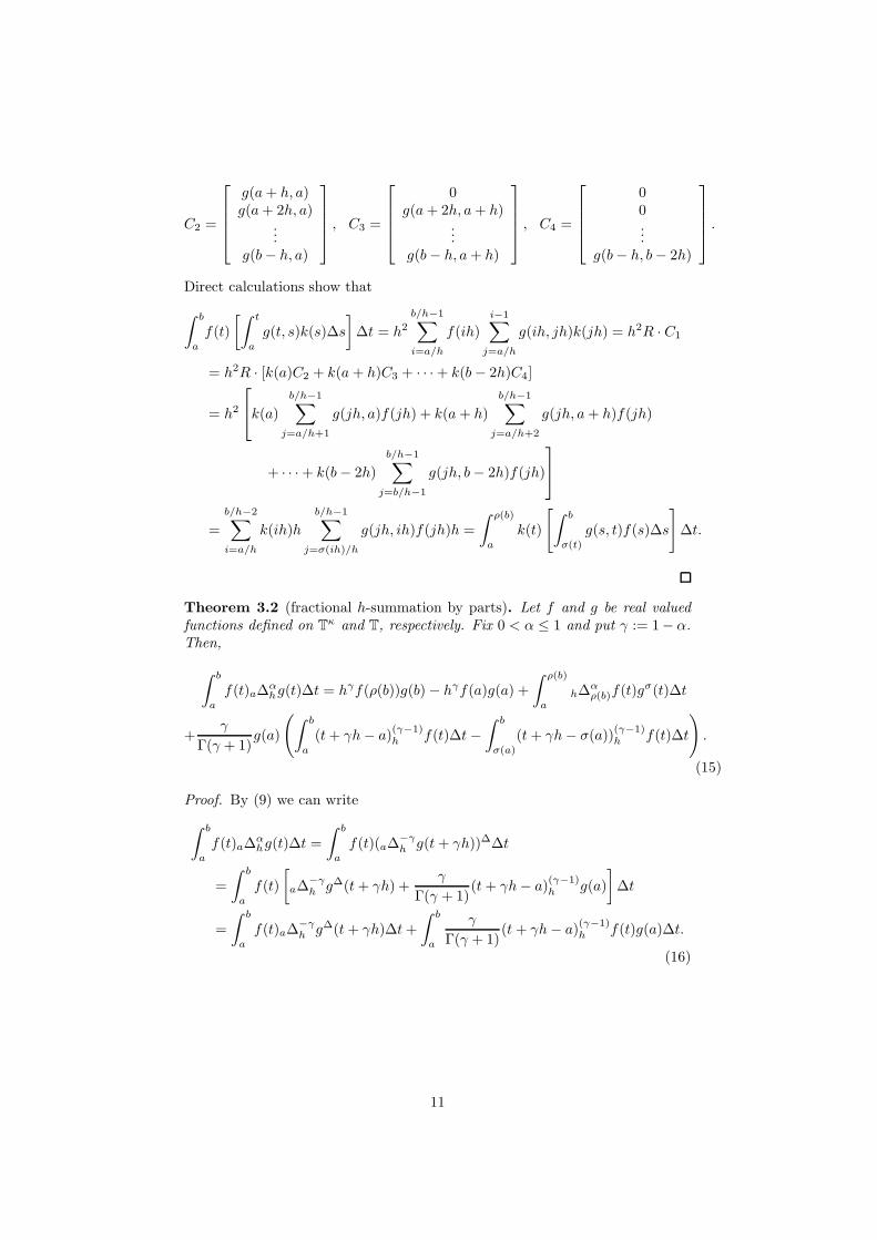
C2 =

g(a+ h, a)g(a+ 2h, a)

...g(b− h, a)

, C3 =

0g(a+ 2h, a+ h)

...g(b− h, a+ h)

, C4 =

00...

g(b− h, b− 2h)

.

Direct calculations show that

∫ b

a

f(t)

[∫ t

a

g(t, s)k(s)∆s

]

∆t = h2

b/h−1∑

i=a/h

f(ih)

i−1∑

j=a/h

g(ih, jh)k(jh) = h2R · C1

= h2R · [k(a)C2 + k(a+ h)C3 + · · ·+ k(b− 2h)C4]

= h2

k(a)

b/h−1∑

j=a/h+1

g(jh, a)f(jh) + k(a+ h)

b/h−1∑

j=a/h+2

g(jh, a+ h)f(jh)

+ · · ·+ k(b− 2h)

b/h−1∑

j=b/h−1

g(jh, b− 2h)f(jh)

=

b/h−2∑

i=a/h

k(ih)h

b/h−1∑

j=σ(ih)/h

g(jh, ih)f(jh)h =

∫ ρ(b)

a

k(t)

[∫ b

σ(t)

g(s, t)f(s)∆s

]

∆t.

Theorem 3.2 (fractional h-summation by parts). Let f and g be real valuedfunctions defined on T

κ and T, respectively. Fix 0 < α ≤ 1 and put γ := 1− α.Then,

∫ b

a

f(t)a∆αhg(t)∆t = hγf(ρ(b))g(b)− hγf(a)g(a) +

∫ ρ(b)

ah∆

αρ(b)f(t)g

σ(t)∆t

+γ

Γ(γ + 1)g(a)

(∫ b

a

(t+ γh− a)(γ−1)h f(t)∆t−

∫ b

σ(a)

(t+ γh− σ(a))(γ−1)h f(t)∆t

)

.

(15)

Proof. By (9) we can write

∫ b

a

f(t)a∆αhg(t)∆t =

∫ b

a

f(t)(a∆−γh g(t+ γh))∆∆t

=

∫ b

a

f(t)

[

a∆−γh g∆(t+ γh) +

γ

Γ(γ + 1)(t+ γh− a)

(γ−1)h g(a)

]

∆t

=

∫ b

a

f(t)a∆−γh g∆(t+ γh)∆t+

∫ b

a

γ

Γ(γ + 1)(t+ γh− a)

(γ−1)h f(t)g(a)∆t.

(16)

11

Using (8) we get∫ b

a

f(t)a∆−γh g∆(t+ γh)∆t

=

∫ b

a

f(t)

[

hγg∆(t) +γ

Γ(γ + 1)

∫ t

a

(t+ γh− σ(s))(γ−1)h g∆(s)∆s

]

∆t

= hγ

∫ b

a

f(t)g∆(t)∆t+γ

Γ(γ + 1)

∫ ρ(b)

a

g∆(t)

∫ b

σ(t)

(s+ γh− σ(t))(γ−1)h f(s)∆s∆t

= hγf(ρ(b))[g(b)− g(ρ(b))] +

∫ ρ(b)

a

g∆(t)h∆−γρ(b)f(t− γh)∆t,

where the third equality follows by Lemma 3.1. We proceed to develop the righthand side of the last equality as follows:

hγf(ρ(b))[g(b)− g(ρ(b))] +

∫ ρ(b)

a

g∆(t)h∆−γρ(b)f(t− γh)∆t

= hγf(ρ(b))[g(b)− g(ρ(b))] +[

g(t)h∆−γρ(b)f(t− γh)

]t=ρ(b)

t=a

−

∫ ρ(b)

a

gσ(t)(h∆−γρ(b)f(t− γh))∆∆t

= hγf(ρ(b))g(b)− hγf(a)g(a)

−γ

Γ(γ + 1)g(a)

∫ b

σ(a)

(s+ γh− σ(a))(γ−1)h f(s)∆s+

∫ ρ(b)

a

(

h∆αρ(b)f(t)

)

gσ(t)∆t,

where the first equality follows from Lemma 2.1. Putting this into (16) we get(15).

3.2. Necessary optimality conditions

We begin to fix two arbitrary real numbers α and β such that α, β ∈ (0, 1].Further, we put γ := 1− α and ν := 1− β.

Let a function L(t, u, v, w) : Tκ × R × R × R → R be given. We considerthe problem of minimizing (or maximizing) a functional L : FT → R subject togiven boundary conditions:

L(y(·)) =

∫ b

a

L(t, yσ(t), a∆αhy(t), h∆

βb y(t))∆t −→ min, y(a) = A, y(b) = B .

(17)Our main aim is to derive necessary optimality conditions for problem (17).

Definition 3.3. For f ∈ FT we define the norm

‖f‖ = maxt∈Tκ

|fσ(t)|+maxt∈Tκ

|a∆αhf(t)|+max

t∈Tκ|h∆

βb f(t)|.

A function y ∈ FT with y(a) = A and y(b) = B is called a local minimum forproblem (17) provided there exists δ > 0 such that L(y) ≤ L(y) for all y ∈ FT

with y(a) = A and y(b) = B and ‖y − y‖ < δ.

Definition 3.4. A function η ∈ FT is called an admissible variation providedη 6= 0 and η(a) = η(b) = 0.

From now on we assume that the second-order partial derivatives Luu, Luv,Luw, Lvw, Lvv, and Lww exist and are continuous.

12

3.2.1. First order optimality condition

Next theorem gives a first order necessary condition for problem (17), i.e.,an Euler-Lagrange type equation for the fractional h-difference setting.

Theorem 3.5 (The h-fractional Euler-Lagrange equation for problem (17)). Ify ∈ FT is a local minimum for problem (17), then the equality

Lu[y](t) + h∆αρ(b)Lv[y](t) + a∆

βhLw[y](t) = 0 (18)

holds for all t ∈ Tκ2

with operator [·] defined by [y](s) = (s, yσ(s), a∆αs y(s), s∆

βb y(s)).

Proof. Suppose that y(·) is a local minimum of L[·]. Let η(·) be an arbitrarily

fixed admissible variation and define a function Φ :(

− δ‖η(·)‖ ,

δ‖η(·)‖

)

→ R by

Φ(ε) = L[y(·) + εη(·)]. (19)

This function has a minimum at ε = 0, so we must have Φ′(0) = 0, i.e.,

∫ b

a

[

Lu[y](t)ησ(t) + Lv[y](t)a∆

αhη(t) + Lw[y](t)h∆

βb η(t)

]

∆t = 0,

which we may write equivalently as

hLu[y](t)ησ(t)|t=ρ(b) +

∫ ρ(b)

a

Lu[y](t)ησ(t)∆t+

∫ b

a

Lv[y](t)a∆αhη(t)∆t

+

∫ b

a

Lw[y](t)h∆βb η(t)∆t = 0. (20)

Using Theorem 3.2 and the fact that η(a) = η(b) = 0, we get

∫ b

a

Lv[y](t)a∆αhη(t)∆t =

∫ ρ(b)

a

(

h∆αρ(b) (Lv[y]) (t)

)

ησ(t)∆t (21)

for the third term in (20). Using (13) it follows that

∫ b

a

Lw[y](t)h∆βb η(t)∆t

=−

∫ b

a

Lw[y](t)(h∆−νb η(t− νh))∆∆t

=−

∫ b

a

Lw[y](t)

[

h∆−νρ(b)η

∆(t− νh)−ν

Γ(ν + 1)(b + νh− σ(t))

(ν−1)h η(b)

]

∆t

=−

∫ b

a

Lw[y](t)h∆−νρ(b)η

∆(t− νh)∆t+νη(b)

Γ(ν + 1)

∫ b

a

(b+ νh− σ(t))(ν−1)h Lw[y](t)∆t.

(22)

13

We now use Lemma 3.1 to get∫ b

a

Lw[y](t)h∆−νρ(b)η

∆(t− νh)∆t

=

∫ b

a

Lw[y](t)

[

hνη∆(t) +ν

Γ(ν + 1)

∫ b

σ(t)

(s+ νh− σ(t))(ν−1)h η∆(s)∆s

]

∆t

=

∫ b

a

hνLw[y](t)η∆(t)∆t

+ν

Γ(ν + 1)

∫ ρ(b)

a

[

Lw[y](t)

∫ b

σ(t)

(s+ νh− σ(t))(ν−1)h η∆(s)∆s

]

∆t

=

∫ b

a

hνLw[y](t)η∆(t)∆t

+ν

Γ(ν + 1)

∫ b

a

[

η∆(t)

∫ t

a

(t+ νh− σ(s))(ν−1)h Lw[y](s)∆s

]

∆t

=

∫ b

a

η∆(t)a∆−νh (Lw[y]) (t+ νh)∆t.

(23)

We apply again the time scale integration by parts formula (Lemma 2.1), thistime to (23), to obtain,∫ b

a

η∆(t)a∆−νh (Lw[y]) (t+ νh)∆t

=

∫ ρ(b)

a

η∆(t)a∆−νh (Lw[y]) (t+ νh)∆t

+ (η(b)− η(ρ(b)))a∆−νh (Lw[y]) (t+ νh)|t=ρ(b)

=[η(t)a∆

−νh (Lw[y]) (t+ νh)

]t=ρ(b)

t=a−

∫ ρ(b)

a

ησ(t)(a∆−νh (Lw[y]) (t+ νh))∆∆t

+ η(b)a∆−νh (Lw[y]) (t+ νh)|t=ρ(b) − η(ρ(b))a∆

−νh (Lw[y]) (t+ νh)|t=ρ(b)

= η(b)a∆−νh (Lw[y]) (t+ νh)|t=ρ(b) − η(a)a∆

−νh (Lw[y]) (t+ νh)|t=a

−

∫ ρ(b)

a

ησ(t)a∆βh (Lw[y]) (t)∆t.

(24)

Since η(a) = η(b) = 0 we obtain, from (23) and (24), that∫ b

a

Lw[y](t)h∆−νρ(b)η

∆(t)∆t = −

∫ ρ(b)

a

ησ(t)a∆βh (Lw[y]) (t)∆t ,

and after inserting in (22), that∫ b

a

Lw[y](t)h∆βb η(t)∆t =

∫ ρ(b)

a

ησ(t)a∆βh (Lw[y]) (t)∆t. (25)

By (21) and (25) we may write (20) as∫ ρ(b)

a

[

Lu[y](t) + h∆αρ(b) (Lv[y]) (t) + a∆

βh (Lw[y]) (t)

]

ησ(t)∆t = 0 .

14

Since the values of ησ(t) are arbitrary for t ∈ Tκ2

, the Euler-Lagrange equation(18) holds along y.

The next result is a direct corollary of Theorem 3.5.

Corollary 3.1 (The h-Euler-Lagrange equation – cf., e.g., [18, 24]). Let T be thetime scale hZ, h > 0, with the forward jump operator σ and the delta derivative∆. Assume a, b ∈ T, a < b. If y is a solution to the problem

L(y(·)) =

∫ b

a

L(t, yσ(t), y∆(t))∆t −→ min, y(a) = A, y(b) = B ,

then the equality Lu(t, yσ(t), y∆(t)) −

(Lv(t, y

σ(t), y∆(t)))∆

= 0 holds for all

t ∈ Tκ2

.

Proof. Choose α = 1 and a L that does not depend on w in Theorem 3.5.

Remark 3.1. If we take h = 1 in Corollary 3.1 we have that

Lu(t, yσ(t),∆y(t))−∆Lv(t, y

σ(t),∆y(t)) = 0

holds for all t ∈ Tκ2

. This equation is usually called the discrete Euler-Lagrangeequation, and can be found, e.g., in [29, Chap. 8].

3.2.2. Natural boundary conditions

If the initial condition y(a) = A is not present in problem (17) (i.e., y(a)is free), besides the h-fractional Euler-Lagrange equation (18) the followingsupplementary condition must be fulfilled:

− hγLv[y](a) +γ

Γ(γ + 1)

(∫ b

a

(t+ γh− a)(γ−1)h Lv[y](t)∆t

−

∫ b

σ(a)

(t+ γh− σ(a))(γ−1)h Lv[y](t)∆t

)

+ Lw[y](a) = 0. (26)

Similarly, if y(b) = B is not present in (17) (y(b) is free), the extra condition

hLu[y](ρ(b)) + hγLv[y](ρ(b))− hνLw[y](ρ(b))

+ν

Γ(ν + 1)

(∫ b

a

(b+ νh− σ(t))(ν−1)h Lw[y](t)∆t

−

∫ ρ(b)

a

(ρ(b) + νh− σ(t))(ν−1)h Lw[y](t)∆t

)

= 0 (27)

is added to Theorem 3.5. We leave the proof of the natural boundary conditions(26) and (27) to the reader. We just note here that the first term in (27) arisesfrom the first term of the left hand side of (20).

15

3.2.3. Second order optimality condition

We now obtain a second order necessary condition for problem (17), i.e.,we prove a Legendre optimality type condition for the fractional h-differencesetting.

Theorem 3.6 (The h-fractional Legendre necessary condition). If y ∈ FT is alocal minimum for problem (17), then the inequality

h2Luu[y](t) + 2hγ+1Luv[y](t) + 2hν+1(ν − 1)Luw[y](t) + h2γ(γ − 1)2Lvv[y](σ(t))

+ 2hν+γ(γ − 1)Lvw[y](σ(t)) + 2hν+γ(ν − 1)Lvw[y](t) + h2ν(ν − 1)2Lww[y](t)

+ h2νLww[y](σ(t)) +

∫ t

a

h3Lww[y](s)

(ν(1 − ν)

Γ(ν + 1)(t+ νh− σ(s))

(ν−2)h

)2

∆s

+ hγLvv[y](t) +

∫ b

σ(σ(t))

h3Lvv[y](s)

(γ(γ − 1)

Γ(γ + 1)(s+ γh− σ(σ(t)))

(γ−2)h

)2

∆s ≥ 0

(28)

holds for all t ∈ Tκ2

, where [y](t) = (t, yσ(t), a∆αt y(t), t∆

βb y(t)).

Proof. By the hypothesis of the theorem, and letting Φ be as in (19), we haveas necessary optimality condition that Φ′′(0) ≥ 0 for an arbitrary admissiblevariation η(·). Inequality Φ′′(0) ≥ 0 is equivalent to

∫ b

a

[

Luu[y](t)(ησ(t))2 + 2Luv[y](t)η

σ(t)a∆αhη(t) + 2Luw[y](t)η

σ(t)h∆βb η(t)

+Lvv[y](t)(a∆αhη(t))

2 + 2Lvw[y](t)a∆αhη(t)h∆

βb η(t) + Lww(t)(h∆

βb η(t))

2]

∆t ≥ 0.

(29)

Let τ ∈ Tκ2

be arbitrary, and choose η : T → R given by η(t) =

{h if t = σ(τ);0 otherwise.

It follows that η(a) = η(b) = 0, i.e., η is an admissible variation. Using (9) weget

∫ b

a

[Luu[y](t)(η

σ(t))2 + 2Luv[y](t)ησ(t)a∆

αhη(t) + Lvv[y](t)(a∆

αhη(t))

2]∆t

=

∫ b

a

[

Luu[y](t)(ησ(t))2

+ 2Luv[y](t)ησ(t)

(

hγη∆(t) +γ

Γ(γ + 1)

∫ t

a

(t+ γh− σ(s))(γ−1)h η∆(s)∆s

)

+ Lvv[y](t)

(

hγη∆(t) +γ

Γ(γ + 1)

∫ t

a

(t+ γh− σ(s))(γ−1)h η∆(s)∆s

)2]

∆t

= h3Luu[y](τ) + 2hγ+2Luv[y](τ) + hγ+1Lvv[y](τ)

+

∫ b

σ(τ)

Lvv[y](t)

(

hγη∆(t) +γ

Γ(γ + 1)

∫ t

a

(t+ γh− σ(s))(γ−1)h η∆(s)∆s

)2

∆t.

16

Observe that

h2γ+1(γ − 1)2Lvv[y](σ(τ))

+

∫ b

σ2(τ)

Lvv[y](t)

(γ

Γ(γ + 1)

∫ t

a

(t+ γh− σ(s))(γ−1)h η∆(s)∆s

)2

∆t

=

∫ b

σ(τ)

Lvv[y](t)

(

hγη∆(t) +γ

Γ(γ + 1)

∫ t

a

(t+ γh− σ(s))(γ−1)h η∆(s)∆s

)2

∆t.

Let t ∈ [σ2(τ), ρ(b)] ∩ hZ. Since

γ

Γ(γ + 1)

∫ t

a

(t+ γh− σ(s))(γ−1)h η∆(s)∆s

=γ

Γ(γ + 1)

[∫ σ(τ)

a

(t+ γh− σ(s))(γ−1)h η∆(s)∆s

+

∫ t

σ(τ)

(t+ γh− σ(s))(γ−1)h η∆(s)∆s

]

= hγ

Γ(γ + 1)

[

(t+ γh− σ(τ))(γ−1)h − (t+ γh− σ(σ(τ)))

(γ−1)h

]

=γhγ

Γ(γ + 1)

[(t−τh + γ − 1

)Γ(t−τh + γ − 1

)−(t−τh

)Γ(t−τh + γ − 1

)

(t−τh

)Γ(t−τh

)

]

= h2 γ(γ − 1)

Γ(γ + 1)(t+ γh− σ(σ(τ)))

(γ−2)h ,

(30)

we conclude that

∫ b

σ2(τ)

Lvv[y](t)

(γ

Γ(γ + 1)

∫ t

a

(t+ γh− σ(s))(γ−1)h η∆(s)∆s

)2

∆t

=

∫ b

σ2(τ)

Lvv[y](t)

(

h2 γ(γ − 1)

Γ(γ + 1)(t+ γh− σ2(τ))

(γ−2)h

)2

∆t.

Note that we can write t∆βb η(t) = −h∆

−νρ(b)η

∆(t − νh) because η(b) = 0. It is

not difficult to see that the following equality holds:∫ b

a

2Luw[y](t)ησ(t)h∆

βb η(t)∆t = −

∫ b

a

2Luw[y](t)ησ(t)h∆

−νρ(b)η

∆(t− νh)∆t

= 2h2+νLuw[y](τ)(ν − 1) .

Moreover,∫ b

a

2Lvw[y](t)a∆αhη(t)h∆

βb η(t)∆t

= −2

∫ b

a

Lvw[y](t)

{(

hγη∆(t) +γ

Γ(γ + 1)·

∫ t

a

(t+ γh− σ(s))(γ−1)h η∆(s)∆s

)

·

[

hνη∆(t) +ν

Γ(ν + 1)

∫ b

σ(t)

(s+ νh− σ(t))(ν−1)h η∆(s)∆s

]}

∆t

= 2hγ+ν+1(ν − 1)Lvw[y](τ) + 2hγ+ν+1(γ − 1)Lvw[y](σ(τ)).

17

Finally, we have that

∫ b

a

Lww[y](t)(h∆βb η(t))

2∆t

=

∫ σ(σ(τ))

a

Lww[y](t)

[

hνη∆(t) +ν

Γ(ν + 1)

∫ b

σ(t)

(s+ νh− σ(t))(ν−1)h η∆(s)∆s

]2

∆t

=

∫ τ

a

Lww[y](t)

[

ν

Γ(ν + 1)

∫ b

σ(t)

(s+ νh− σ(t))(ν−1)h η∆(s)∆s

]2

∆t

+ hLww[y](τ)(hν − νhν)2 + h2ν+1Lww[y](σ(τ))

=

∫ τ

a

Lww[y](t)

[

hν

Γ(ν + 1)

{

(τ + νh− σ(t))(ν−1)h − (σ(τ) + νh− σ(t))

(ν−1)h

}]2

+ hLww[y](τ)(hν − νhν)2 + h2ν+1Lww[y](σ(τ)).

Similarly as we did in (30), we can prove that

hν

Γ(ν + 1)

{

(τ + νh− σ(t))(ν−1)h − (σ(τ) + νh− σ(t))

(ν−1)h

}

= h2 ν(1− ν)

Γ(ν + 1)(τ + νh− σ(t))

(ν−2)h .

Thus, we have that inequality (29) is equivalent to

h

{

h2Luu[y](t) + 2hγ+1Luv[y](t) + hγLvv[y](t) + Lvv(σ(t))(γhγ − hγ)2

+

∫ b

σ(σ(t))

h3Lvv(s)

(γ(γ − 1)

Γ(γ + 1)(s+ γh− σ(σ(t)))

(γ−2)h

)2

∆s

+ 2hν+1Luw[y](t)(ν − 1) + 2hγ+ν(ν − 1)Lvw[y](t)

+ 2hγ+ν(γ − 1)Lvw(σ(t)) + h2νLww[y](t)(1 − ν)2 + h2νLww[y](σ(t))

+

∫ t

a

h3Lww[y](s)

(ν(1 − ν)

Γ(ν + 1)(t+ νh− σ(s))ν−2

)2

∆s

}

≥ 0. (31)

Because h > 0, (31) is equivalent to (28). The theorem is proved.

The next result is a simple corollary of Theorem 3.6.

Corollary 3.2 (The h-Legendre necessary condition – cf. Result 1.3 of [18]).Let T be the time scale hZ, h > 0, with the forward jump operator σ and thedelta derivative ∆. Assume a, b ∈ T, a < b. If y is a solution to the problem

L(y(·)) =

∫ b

a

L(t, yσ(t), y∆(t))∆t −→ min, y(a) = A, y(b) = B ,

then the inequality

h2Luu[y](t) + 2hLuv[y](t) + Lvv[y](t) + Lvv[y](σ(t)) ≥ 0 (32)

holds for all t ∈ Tκ2

, where [y](t) = (t, yσ(t), y∆(t)).

18

Proof. Choose α = 1 and a Lagrangian L that does not depend on w. Then,γ = 0 and the result follows immediately from Theorem 3.6.

Remark 3.2. When h goes to zero we have σ(t) = t and inequality (32) coin-cides with Legendre’s classical necessary optimality condition Lvv[y](t) ≥ 0 (cf.,e.g., [50]).

4. Examples

In this section we present some illustrative examples.

Example 4.1. Let us consider the following problem:

L(y) =1

2

∫ 1

0

(

0∆34

h y(t))2

∆t −→ min , y(0) = 0 , y(1) = 1 . (33)

We consider (33) with different values of h. Numerical results show that whenh tends to zero the h-fractional Euler-Lagrange extremal tends to the fractionalcontinuous extremal: when h → 0 (33) tends to the fractional continuous vari-ational problem in the Riemann-Liouville sense studied in [1, Example 1], withsolution given by

y(t) =1

2

∫ t

0

dx

[(1 − x)(t− x)]14

. (34)

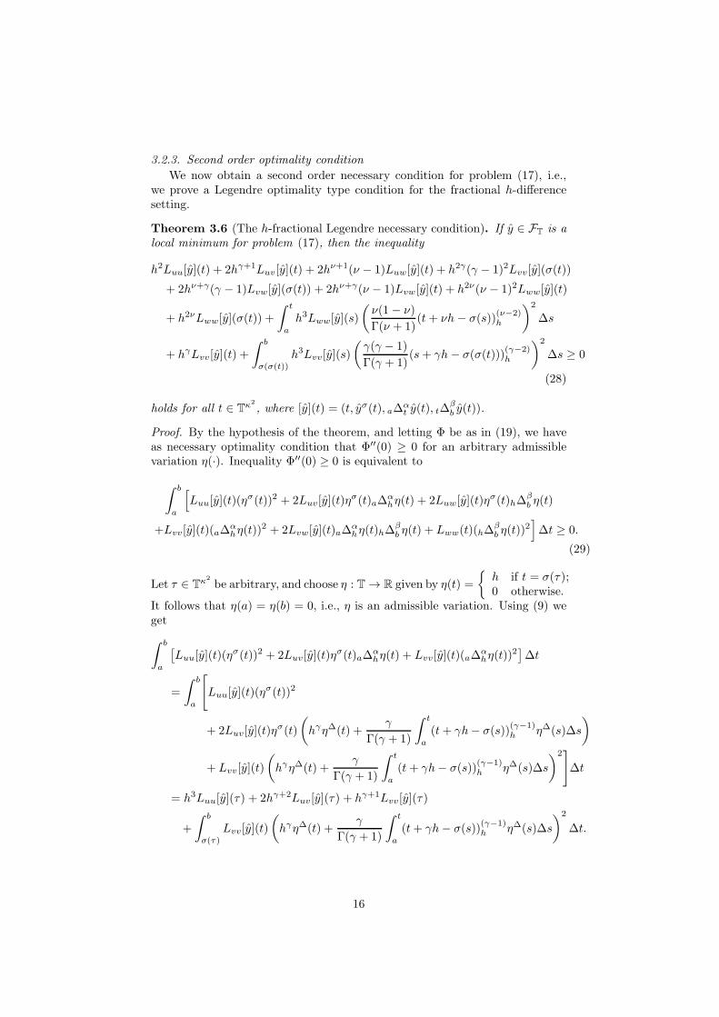
This is illustrated in Figure 1. In this example for each value of h there is

0

0.1

0.2

0.3

0.4

0.5

0.6

0.7

0.8

0.9

1.0

0 1

b

b

b

+

+

+

+

+

+

+

+

+

*

*

**

**

**

**

**

*

*

*

*

*

××

××

×× × × × × × × × × × × × × × × × ×

××

××

××

××

×

y(t)

t

Figure 1: Extremal y(t) for problem of Example 4.1 with different values of h: h = 0.50 (•);h = 0.125 (+); h = 0.0625 (∗); h = 1/30 (×). The continuous line represent function (34).

a unique h-fractional Euler-Lagrange extremal, solution of (18), which alwaysverifies the h-fractional Legendre necessary condition (28).

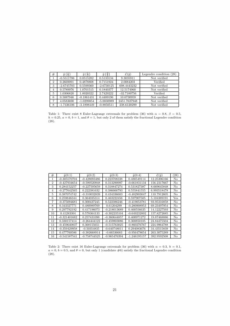
Example 4.2. Let us consider the following problem:

L(y) =

∫ 1

0

[1

2(0∆

αhy(t))

2 − yσ(t)

]

∆t −→ min , y(0) = 0 , y(1) = 0 . (35)

We begin by considering problem (35) with a fixed value for α and differentvalues of h. The extremals y are obtained using our Euler-Lagrange equation

19

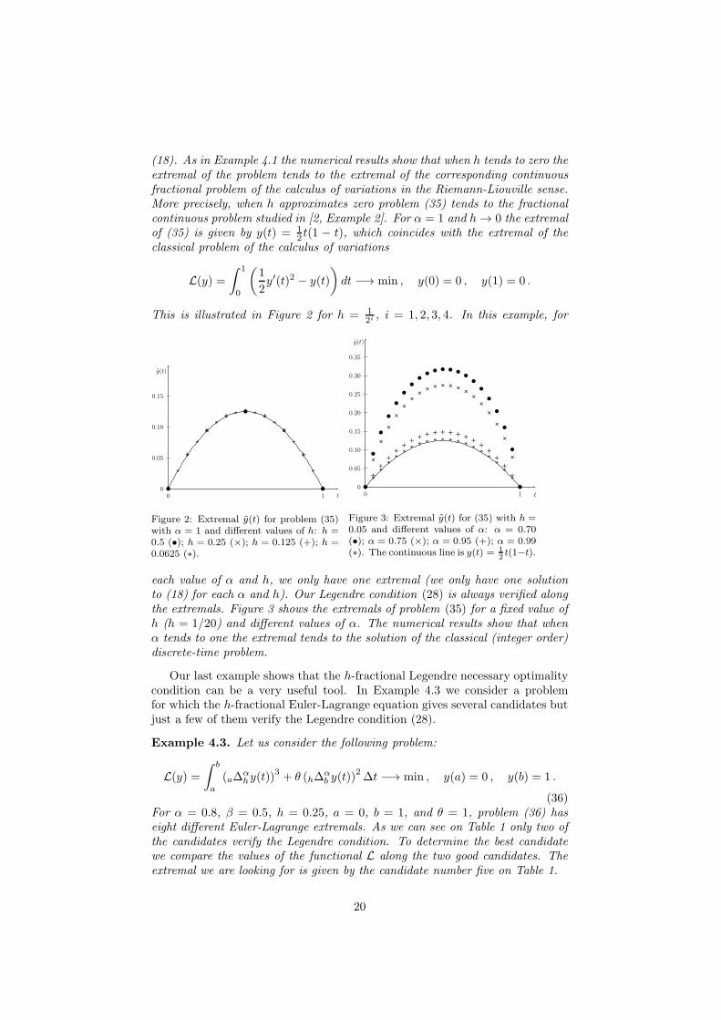
(18). As in Example 4.1 the numerical results show that when h tends to zero theextremal of the problem tends to the extremal of the corresponding continuousfractional problem of the calculus of variations in the Riemann-Liouville sense.More precisely, when h approximates zero problem (35) tends to the fractionalcontinuous problem studied in [2, Example 2]. For α = 1 and h → 0 the extremalof (35) is given by y(t) = 1

2 t(1 − t), which coincides with the extremal of theclassical problem of the calculus of variations

L(y) =

∫ 1

0

(1

2y′(t)2 − y(t)

)

dt −→ min , y(0) = 0 , y(1) = 0 .

This is illustrated in Figure 2 for h = 12i , i = 1, 2, 3, 4. In this example, for

0

0.05

0.10

0.15

0 1

b

b

b×

×

×

×

×+

+

+

+ + +

+

+

+*

*

*

*

**

* * * * **

*

*

*

*

*

y(t)

t

Figure 2: Extremal y(t) for problem (35)with α = 1 and different values of h: h =0.5 (•); h = 0.25 (×); h = 0.125 (+); h =0.0625 (∗).

0

0.05

0.10

0.15

0.20

0.25

0.30

0.35

0 1

b

b

b

b

b

b

bb

bb b b b

bb

b

b

b

b

b

b×

×

×

×

××

×× × × × × × ×

××

×

×

×

×

×++

++

++ + + + + + + + + + +

++

++

+**

**

**

* * * * * * * * **

**

**

*

y(t)

t

Figure 3: Extremal y(t) for (35) with h =0.05 and different values of α: α = 0.70(•); α = 0.75 (×); α = 0.95 (+); α = 0.99(∗). The continuous line is y(t) = 1

2t(1−t).

each value of α and h, we only have one extremal (we only have one solutionto (18) for each α and h). Our Legendre condition (28) is always verified alongthe extremals. Figure 3 shows the extremals of problem (35) for a fixed value ofh (h = 1/20) and different values of α. The numerical results show that whenα tends to one the extremal tends to the solution of the classical (integer order)discrete-time problem.

Our last example shows that the h-fractional Legendre necessary optimalitycondition can be a very useful tool. In Example 4.3 we consider a problemfor which the h-fractional Euler-Lagrange equation gives several candidates butjust a few of them verify the Legendre condition (28).

Example 4.3. Let us consider the following problem:

L(y) =

∫ b

a

(a∆αhy(t))

3+ θ (h∆

αb y(t))

2∆t −→ min , y(a) = 0 , y(b) = 1 .

(36)For α = 0.8, β = 0.5, h = 0.25, a = 0, b = 1, and θ = 1, problem (36) haseight different Euler-Lagrange extremals. As we can see on Table 1 only two ofthe candidates verify the Legendre condition. To determine the best candidatewe compare the values of the functional L along the two good candidates. Theextremal we are looking for is given by the candidate number five on Table 1.

20

# y(

1

4

)

y(

1

2

)

y(

3

4

)

L(y) Legendre condition (28)

1 -0.5511786 0.0515282 0.5133134 9.3035911 Not verified2 0.2669091 0.4878808 0.7151924 2.0084203 Verified3 -2.6745703 0.5599360 -2.6730125 698.4443232 Not verified4 0.5789976 1.0701515 0.1840377 12.5174960 Not verified5 1.0306820 1.8920322 2.7429222 -32.7189756 Verified6 0.5087946 -0.1861431 0.4489196 10.6730959 Not verified7 4.0583690 -1.0299054 -5.0030989 2451.7637948 Not verified8 -1.7436106 -3.1898449 -0.8850511 238.6120299 Not verified

Table 1: There exist 8 Euler-Lagrange extremals for problem (36) with α = 0.8, β = 0.5,h = 0.25, a = 0, b = 1, and θ = 1, but only 2 of them satisfy the fractional Legendre condition(28).

# y(0.1) y(0.2) y(0.3) y(0.4) L(y) (28)1 -0.305570704 -0.428093486 0.223708338 0.480549114 12.25396166 No2 -0.427934654 -0.599520948 0.313290997 -0.661831134 156.2317667 No3 0.284152257 -0.227595659 0.318847274 0.531827387 8.669645848 No4 -0.277642565 0.222381632 0.386666793 0.555841555 6.993518478 No5 0.387074742 -0.310032839 0.434336603 -0.482903047 110.7912605 No6 0.259846344 0.364035314 0.463222456 0.597907505 5.104389191 Yes7 -0.375094681 0.300437245 0.522386246 -0.419053781 93.95316858 No8 0.343327771 0.480989769 0.61204299 -0.280908953 69.23497954 No9 0.297792192 0.417196073 -0.218013689 0.460556635 14.12227593 No10 0.41283304 0.578364133 -0.302235104 -0.649232892 157.8272685 No11 -0.321401682 0.257431098 -0.360644857 0.400971272 19.87468886 No12 0.330157414 -0.264444122 -0.459803086 0.368850105 24.84475504 No13 -0.459640837 0.368155651 -0.515763025 -0.860276767 224.9964788 No14 -0.359429958 -0.50354835 -0.640748011 0.294083676 34.43515839 No15 0.477760586 -0.382668914 -0.66536683 -0.956478654 263.3075289 No16 -0.541587541 -0.758744525 -0.965476394 -1.246195157 392.9592508 No

Table 2: There exist 16 Euler-Lagrange extremals for problem (36) with α = 0.3, h = 0.1,a = 0, b = 0.5, and θ = 0, but only 1 (candidate #6) satisfy the fractional Legendre condition(28).

21

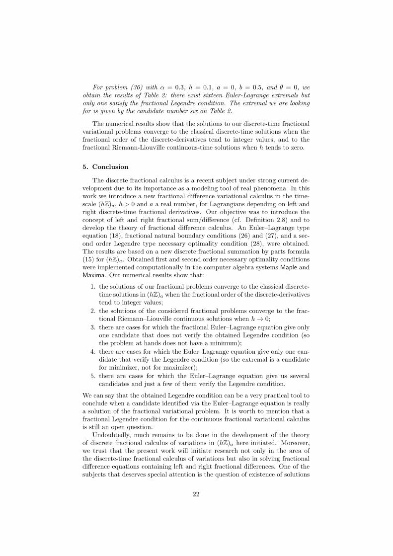
For problem (36) with α = 0.3, h = 0.1, a = 0, b = 0.5, and θ = 0, weobtain the results of Table 2: there exist sixteen Euler-Lagrange extremals butonly one satisfy the fractional Legendre condition. The extremal we are lookingfor is given by the candidate number six on Table 2.

The numerical results show that the solutions to our discrete-time fractionalvariational problems converge to the classical discrete-time solutions when thefractional order of the discrete-derivatives tend to integer values, and to thefractional Riemann-Liouville continuous-time solutions when h tends to zero.

5. Conclusion

The discrete fractional calculus is a recent subject under strong current de-velopment due to its importance as a modeling tool of real phenomena. In thiswork we introduce a new fractional difference variational calculus in the time-scale (hZ)a, h > 0 and a a real number, for Lagrangians depending on left andright discrete-time fractional derivatives. Our objective was to introduce theconcept of left and right fractional sum/difference (cf. Definition 2.8) and todevelop the theory of fractional difference calculus. An Euler–Lagrange typeequation (18), fractional natural boundary conditions (26) and (27), and a sec-ond order Legendre type necessary optimality condition (28), were obtained.The results are based on a new discrete fractional summation by parts formula(15) for (hZ)a. Obtained first and second order necessary optimality conditionswere implemented computationally in the computer algebra systems Maple andMaxima. Our numerical results show that:

1. the solutions of our fractional problems converge to the classical discrete-time solutions in (hZ)a when the fractional order of the discrete-derivativestend to integer values;

2. the solutions of the considered fractional problems converge to the frac-tional Riemann–Liouville continuous solutions when h → 0;

3. there are cases for which the fractional Euler–Lagrange equation give onlyone candidate that does not verify the obtained Legendre condition (sothe problem at hands does not have a minimum);

4. there are cases for which the Euler–Lagrange equation give only one can-didate that verify the Legendre condition (so the extremal is a candidatefor minimizer, not for maximizer);

5. there are cases for which the Euler–Lagrange equation give us severalcandidates and just a few of them verify the Legendre condition.

We can say that the obtained Legendre condition can be a very practical tool toconclude when a candidate identified via the Euler–Lagrange equation is reallya solution of the fractional variational problem. It is worth to mention that afractional Legendre condition for the continuous fractional variational calculusis still an open question.

Undoubtedly, much remains to be done in the development of the theoryof discrete fractional calculus of variations in (hZ)a here initiated. Moreover,we trust that the present work will initiate research not only in the area ofthe discrete-time fractional calculus of variations but also in solving fractionaldifference equations containing left and right fractional differences. One of thesubjects that deserves special attention is the question of existence of solutions

22

to the discrete fractional Euler–Lagrange equations. Note that the obtainedfractional equation (18) involves both the left and the right discrete fractionalderivatives. Other interesting directions of research consist to study optimalityconditions for more general variable endpoint variational problems [28, 34, 35];isoperimetric problems [5, 6]; higher-order problems of the calculus of variations[12, 24, 38]; to obtain fractional sufficient optimality conditions of Jacobi typeand a version of Noether’s theorem [17, 21, 25, 27] for discrete-time fractionalvariational problems; direct methods of optimization for absolute extrema [19,36, 49]; to generalize our fractional first and second order optimality conditionsfor a fractional Lagrangian possessing delay terms [14, 37]; and to generalize theresults from (hZ)a to an arbitrary time scale T.

Acknowledgments

This work is part of the first author’s PhD project carried out at the Uni-versity of Aveiro under the framework of the Doctoral Programme Mathe-matics and Applications of Universities of Aveiro and Minho. The financialsupport of the Polytechnic Institute of Viseu and The Portuguese Founda-tion for Science and Technology (FCT), through the “Programa de apoio aformacao avancada de docentes do Ensino Superior Politecnico”, PhD fellowshipSFRH/PROTEC/49730/2009, is here gratefully acknowledged. The second au-thor was supported by FCT through the PhD fellowship SFRH/BD/39816/2007;the third author by FCT through the R&D unit Centre for Research on Opti-mization and Control (CEOC) and the project UTAustin/MAT/0057/2008.

[1] O. P. Agrawal, Formulation of Euler-Lagrange equations for fractional vari-ational problems, J. Math. Anal. Appl. 272 (2002), no. 1, 368–379.

[2] O. P. Agrawal, A general finite element formulation for fractional varia-tional problems, J. Math. Anal. Appl. 337 (2008), no. 1, 1–12.

[3] O. P. Agrawal and D. Baleanu, A Hamiltonian formulation and a directnumerical scheme for fractional optimal control problems, J. Vib. Control13 (2007), no. 9-10, 1269–1281.

[4] R. Almeida, A. B. Malinowska and D. F. M. Torres, A fractional calculusof variations for multiple integrals with application to vibrating string, J.Math. Phys. 51 (2010), no. 3, 033503, 12 pp. arXiv:1001.2722

[5] R. Almeida and D. F. M. Torres, Holderian variational problems subjectto integral constraints, J. Math. Anal. Appl. 359 (2009), no. 2, 674–681.arXiv:0807.3076

[6] R. Almeida and D. F. M. Torres, Isoperimetric problems on time scaleswith nabla derivatives, J. Vib. Control 15 (2009), no. 6, 951–958.arXiv:0811.3650

[7] R. Almeida and D. F. M. Torres, Calculus of variations with fractionalderivatives and fractional integrals, Appl. Math. Lett. 22 (2009), no. 12,1816–1820. arXiv:0907.1024

[8] F. M. Atici and P. W. Eloe, A transform method in discrete fractionalcalculus, Int. J. Difference Equ. 2 (2007), no. 2, 165–176.

23

[9] F. M. Atici and P. W. Eloe, Initial value problems in discrete fractionalcalculus, Proc. Amer. Math. Soc. 137 (2009), no. 3, 981–989.

[10] D. Baleanu, New applications of fractional variational principles, Rep.Math. Phys. 61 (2008), no. 2, 199–206.

[11] D. Baleanu, O. Defterli and O. P. Agrawal, A central difference numericalscheme for fractional optimal control problems, J. Vib. Control 15 (2009),no. 4, 583–597.

[12] D. Baleanu and F. Jarad, Discrete variational principles for higher-orderLagrangians, Nuovo Cimento Soc. Ital. Fis. B 120 (2005), no. 9, 931–938.

[13] D. Baleanu and F. Jarad, Difference discrete variational principles, inMath-ematical analysis and applications, 20–29, Amer. Inst. Phys., Melville, NY,2006.

[14] D. Baleanu, T. Maaraba and F. Jarad, Fractional variational principleswith delay, J. Phys. A 41 (2008), no. 31, 315403, 8 pp.

[15] D. Baleanu and S. I. Muslih, Nonconservative systems within fractionalgeneralized derivatives, J. Vib. Control 14 (2008), no. 9-10, 1301–1311.

[16] D. Baleanu, S. I. Muslih and E. M. Rabei, On fractional Euler-Lagrange andHamilton equations and the fractional generalization of total time deriva-tive, Nonlinear Dynam. 53 (2008), no. 1-2, 67–74.

[17] Z. Bartosiewicz and D. F. M. Torres, Noether’s theorem on time scales, J.Math. Anal. Appl. 342 (2008), no. 2, 1220–1226. arXiv:0709.0400

[18] M. Bohner, Calculus of variations on time scales, Dynam. Systems Appl.13 (2004), 339–349.

[19] M. Bohner, R. A. C. Ferreira and D. F. M. Torres, Integral inequalitiesand their applications to the calculus of variations on time scales, Math.Inequal. Appl. 13 (2010), no. 3, 511–522. arXiv:1001.3762

[20] M. Bohner and A. Peterson, Dynamic equations on time scales, Birkhauser,Boston, MA, 2001.

[21] J. Cresson, G. S. F. Frederico and D. F. M. Torres, Constants of motionfor non-differentiable quantum variational problems, Topol. Methods Non-linear Anal. 33 (2009), no. 2, 217–231. arXiv:0805.0720

[22] R. A. El-Nabulsi and D. F. M. Torres, Necessary optimality conditionsfor fractional action-like integrals of variational calculus with Riemann-Liouville derivatives of order (α, β), Math. Methods Appl. Sci. 30 (2007),no. 15, 1931–1939. arXiv:math-ph/0702099

[23] R. A. El-Nabulsi and D. F. M. Torres, Fractional actionlike variationalproblems, J. Math. Phys. 49 (2008), no. 5, 053521, 7 pp. arXiv:0804.4500

[24] R. A. C. Ferreira and D. F. M. Torres, Higher-order calculus of variations ontime scales, in Mathematical control theory and finance, 149–159, Springer,Berlin, 2008. arXiv:0706.3141

24

[25] G. S. F. Frederico and D. F. M. Torres, A formulation of Noether’s theoremfor fractional problems of the calculus of variations, J. Math. Anal. Appl.334 (2007), no. 2, 834–846. arXiv:math.OC/0701187

[26] G. S. F. Frederico and D. F. M. Torres, Fractional conservation lawsin optimal control theory, Nonlinear Dynam. 53 (2008), no. 3, 215–222.arXiv:0711.0609

[27] G. S. F. Frederico and D. F. M. Torres, Fractional Noether’s theo-rem in the Riesz-Caputo sense, Appl. Math. Comput. (2010), in press.DOI:10.1016/j.amc.2010.01.100 arXiv:1001.4507

[28] R. Hilscher and V. Zeidan, Calculus of variations on time scales: weak localpiecewise C1

rd solutions with variable endpoints, J. Math. Anal. Appl. 289(2004), no. 1, 143–166.

[29] W. G. Kelley and A. C. Peterson, Difference equations, Academic Press,Boston, MA, 1991.

[30] A. A. Kilbas, H. M. Srivastava and J. J. Trujillo, Theory and applicationsof fractional differential equations, Elsevier, Amsterdam, 2006.

[31] F. Jarad and D. Baleanu, Discrete variational principles for Lagrangianslinear in velocities, Rep. Math. Phys. 59 (2007), no. 1, 33–43.

[32] F. Jarad, D. Baleanu and T. Maraaba, Hamiltonian formulation of singularLagrangians on time scales, Chinese Phys. Lett. 25 (2008), no. 5, 1720–1723.

[33] A. B. Malinowska and D. F. M. Torres, Strong minimizers of the calculusof variations on time scales and the Weierstrass condition, Proc. Est. Acad.Sci. 58 (2009), no. 4, 205–212. arXiv:0905.1870

[34] A. B. Malinowska and D. F. M. Torres, Natural boundary conditions inthe calculus of variations, Math. Methods Appl. Sci. (2010), in press.DOI:10.1002/mma.1289 arXiv:0812.0705

[35] A. B. Malinowska and D. F. M. Torres, Generalized natural boundary con-ditions for fractional variational problems in terms of the Caputo derivative,Comput. Math. Appl. 59 (2010), no. 9, 3110–3116. arXiv:1002.3790

[36] A. B. Malinowska and D. F. M. Torres, Leitmann’s direct method ofoptimization for absolute extrema of certain problems of the calculus ofvariations on time scales, Appl. Math. Comput. (2010), in press. DOI:10.1016/j.amc.2010.01.015 arXiv:1001.1455

[37] T. Maraaba, F. Jarad and D. Baleanu, Variational optimal-control prob-lems with delayed arguments on time scales, Adv. Difference Equ. 2009,Art. ID 840386, 15 pp.

[38] N. Martins and D. F. M. Torres, Calculus of variations on time scaleswith nabla derivatives, Nonlinear Anal. 71 (2009), no. 12, e763–e773.arXiv:0807.2596

25

[39] K. S. Miller and B. Ross, Fractional difference calculus, in Univalent func-tions, fractional calculus, and their applications (Koriyama, 1988), 139–152, Horwood, Chichester, 1989.

[40] K. S. Miller and B. Ross, An introduction to the fractional calculus andfractional differential equations, Wiley, New York, 1993.

[41] S. I. Muslih and D. Baleanu, Fractional Euler-Lagrange equations of motionin fractional space, J. Vib. Control 13 (2007), no. 9-10, 1209–1216.

[42] M. D. Ortigueira, Fractional central differences and derivatives, J. Vib.Control 14 (2008), no. 9-10, 1255–1266.

[43] I. Podlubny, Fractional differential equations, Academic Press, San Diego,CA, 1999.

[44] E. M. Rabei, K. I. Nawafleh, R. S. Hijjawi, S. I. Muslih and D. Baleanu,The Hamilton formalism with fractional derivatives, J. Math. Anal. Appl.327 (2007), no. 2, 891–897.

[45] E. M. Rabei, D. M. Tarawneh, S. I. Muslih and D. Baleanu, Heisenberg’sequations of motion with fractional derivatives, J. Vib. Control 13 (2007),no. 9-10, 1239–1247.

[46] B. Ross, S. G. Samko and E. R. Love, Functions that have no first orderderivative might have fractional derivatives of all orders less than one, RealAnal. Exchange 20 (1994), 140–157.

[47] S. G. Samko, A. A. Kilbas and O. I. Marichev, Fractional integrals andderivatives, Translated from the 1987 Russian original, Gordon and Breach,Yverdon, 1993.

[48] M. F. Silva, J. A. Tenreiro Machado and R. S. Barbosa, Using fractionalderivatives in joint control of hexapod robots, J. Vib. Control 14 (2008),no. 9-10, 1473–1485.

[49] D. F. M. Torres and G. Leitmann, Contrasting two transformation-basedmethods for obtaining absolute extrema, J. Optim. Theory Appl. 137

(2008), no. 1, 53–59. arXiv:0704.0473

[50] B. van Brunt, The calculus of variations, Springer, New York, 2004.

26