Statistics 910, #18 1

Discrete Fourier Transform

Overview

1. Review of spectral representation

2. Harmonic regression

3. Discrete Fourier transform

4. Examples of the DFT

5. Periodogram

6. Hibert space perspective

7. Examples

Review of Spectral Representation

Spectral representation of a stationary process {Xt} is

Xt =∫ 1/2

−1/2e2πı tλZ(dλ) , (1)

where Z represents a right-continuous, complex-valued random pro-cess with orthogonal increments for which Var Z(dλ) = dF (λ). Thecovariances are

γ(h) = E Xt+h Xt =∫ 1/2

−1/2e2πı hλdF (λ) . (2)

If F is absolutely continuous with derivative dF (λ)/dλ = f(λ), then

γ(h) =∫ 1/2

−1/2e2πı hλf(λ)dλ and f(λ) =

∞∑h=−∞

γ(h)e−2πı λh (3)

For real-valued processes, f(λ) is symmetric about λ = 0.

Statistics 910, #18 2

Anova interpretation Since the variance of {Xt} has the representation

Var(Xt) = γ(0) =∫ 1/2

−1/2f(λ)dλ ,

the spectral density represents a decomposition of variance into fre-quency intervals. Just as a pdf measures probability in intervals, the“power spectrum” f(λ) shows the distribution of variance over fre-quency.

Review: Harmonic regression

Regression on sinusoids Regression models with sines and cosines arethe underlying statistical models used in frequency domain analysisof time series. Consider a regression model that mimics the randomphase model,

Xt = µ+R cos(2πλt+ ϕ) + wt= µ+R (cos(2πλt) cosϕ)− sin(2πλt) sinϕ) + wt= µ+A cos 2πλt+B sin 2πλt+ wt

where A = R cosϕ and B = −R sinϕ; R2 = A2 + B2 is the squaredamplitude of the sinusoid at frequency λ. The period associated withthe frequency λ is 1/λ. (Alternatively, one can use angular frequencies,being 2π times the usual frequency. I intend to reserve the symbol ωfor angular frequencies.)

Aliasing The frequency is restricted to the range −1/2 < λ ≤ 1/2. Fordiscrete data, frequencies outside of this range are aliased into thisrange. For example, suppose that 1

2 < (λ = 1− δ) < 1, then

cos(2πλt) = cos(2π(1− δ)t)= cos(2πt) cos(2πδt) + sin(2πt) sin(2πδt)= cos 2πδt .

A sampled sinusoid with frequency higher than 12 appears as a sinusoid

with frequency in the interval [0, 1/2]. 12 is known as the folding fre-

quency; we have to see two samples to estimate the energy associatedwith a sinusoid.

Statistics 910, #18 3

Fourier frequencies and orthogonality The frequency −12 < λ ≤ 1

2 isknown as a Fourier frequency if the associated sinusoid completes aninteger number of cycles in the observed length of data. Since theperiod is 1/λ, Fourier frequencies have the form (assuming n is even)

λj =j

n, j = 0, 1, 2, . . . , n/2, (4)

Because of aliasing, the set of j’s stop at n/2. The advantage ofconsidering the Fourier frequencies is that they generate an orthogonalset of regressors. For sines/cosines, we have

n∑t=1

cos2(2πλjt) =

{n j = 0, n/2n/2 j = 1, . . . , n/2− 1

n∑t=1

sin2(2πλjt) =

{0 j = 0, n/2n/2 j = 1, . . . , n/2− 1

n∑t=1

cos(2πλkt) sin(2πλjt) = 0

Harmonic regression If we use Fourier frequencies in our harmonic re-gression, the regression coefficients are easily found since “X ′X” isdiagonal. Consider the coefficients in the harmonic regression (n even)

Xt = A0 +n/2−1∑j=0

Aj cos(2πλjt) +Bj sin(2πλjt) +An/2 (5)

where we define the coefficients (which are also the least squares esti-mates)

A0 =∑t

Xt/n An/2 =∑t

Xt(−1)t/n

Aj =2n

∑t

Xt cos 2πλjt Bj =2n

∑t

Xt sin 2πλjt .

Note that B0 = Bn/2 = 0; there is no imaginary/sine component forthese terms. The sum of squares captured by a specific sine/cosinepair at frequency λj (j 6= 0, n/2) is (recall in OLS regression that theregression SS is β̂′X ′Xβ̂)

Regr SSj =n

2(A2

j +B2j ) =

n

2R2j . (6)

Statistics 910, #18 4

The amplitude of the fitted sinusoid Rj determines the variance ex-plained by this term in a regression model.

Orthogonal transformation Since the harmonic regression 5 includes all1 + n

2 Fourier frequencies from zero to 12 , this regression fits n pa-

rameters to n observations X1, . . . , Xn. This is not estimation; it’s atransformation. The model fits perfectly. Thus the variation in thefitted values is exactly that of the original data, and we obtain thefollowing decomposition of the variance by adding up the regressionsum-of-squares (6) attributed to each frequency:

∑t

X2t = n(R2

0 +R2n/2) +

n

2

n/2−1∑j=1

R2j , (7)

The weights on R0 and Rn/2 differ since there is no sine term at thesefrequencies.

Hilbert space The data X = (X1, . . . , Xn)′ form a vector in n-dimensionalspace. The usual basis for this space is the set of vectors

1j = (0 . . . 0 0 1j 0 0 . . . 0).

Thus we can write X =∑

tXt1t. The harmonic model uses a differ-ent orthogonal basis, namely the sines and cosines associated with theFourier frequencies. The “saturated” harmonic regression (5) repre-sents X in this new basis. The coordinates of X in this basis are thecoefficients Aj and Bj . Since we are writing the same vector X in twodifferent coordinate systems (that are both orthogonal), the length ofthe vector does not change. Thus we must have the equivalence oflengths evident in (7), which is Parseval’s equality in the context ofharmonic regression.

Changing to complex variables leads to the discrete Fourier transform.

Discrete Fourier transform

Definition The discrete Fourier transform (DFT) of the real-valued n-term sequence X0, . . . , Xn−1 is defined as (zero-based indexing on the

Statistics 910, #18 5

data from 0 to n− 1 is more convenient with the DFT)

Jn,j =1n

n−1∑t=0

Xte−2πı λjt, j = 0, 1, 2, . . . , n− 1. (8)

The DFT is the set of harmonic regression coefficients, written usingcomplex variables. For j = 0, 1, . . . , n2 ,

Jn,j =1n

n−1∑t=0

Xte−2πı λjt

=12

(2n

n−1∑t=0

Xt cos(2πλjt)− iXt sin(2πλjt)

)=

12

(Aj − iBj)

Caution: There are many conventions for the leading divisor. S&Sdefine the DFT with leading divisor 1/

√n and R omits this factor

altogether. Always test your software (e.g., take the transform of thesequence 1,1 and see if the leading term is 1,

√2, or 2).

Matrix form As with harmonic regression, the DFT amounts to a changeof basis transformation. Define the n× n matrix Fn,jk = e2πı jk/n andnote F ∗nFn = n In (∗ denotes the conjugate of the transpose). We canthen express the transform as

Jn =1nF ∗nY . (9)

Fast Fourier transform (FFT) is an algorithm for evaluating the matrixmultiplication (9) (which appears to be of order n2) in order n log noperations by a clever recursion (which is basically Horner’s rule forevaluating a polynomial). Here’s the idea.

The DFT of a sequence {x0, x1} of length n = 2 is easy: J2, 0 =(x0 + x1)/2 and J2, 1 = (x1 − x2)/2. Now consider the DFT of thesequence {x0, x1, x2, x3:

3∑t=0

xte−2πı jt/4 = (x0 + x2e

−2πı 2j/4) + (x1e−2πı j/4 + x3e

−2πı 3j/4

= (x0 + x2e−2πı j/2) + e−2πı j/4(x1 + x3e

−2πı j/2)

Statistics 910, #18 6

You can see that the DFT of a sequence of 4 numbers can be writtenin terms of two DFTs of length 2, applied to the even-indexed andodd-indexed elements. This recursion works in general: the DFT ofa sequence of n can be written (for even n) as a sum of the DFTof the even and odd-indexed elements. So what? Count the numberof operations: if n = 2N is a power of two, you require O(n log2 n)operations rather than O(n2). Wavelets take this one step farther,requiring order O(n) operations.

Properties of the DFT

Linearity Since it’s a linear transformation (matrix multiplication, a changeof basis), the DFT is a linear operator. e.g., the DFT of a sum is thesum of the DFT’s:

Jx+yn,j =1n

∑t

(xt + yt)e−2πı λjt = Jxn,j + Jyn,j .

Thus, once we understand how the DFT behaves for some simple series,we can understand it for any others that are sums of these simple cases.

Real-valued data Since we begin with n real-valued observations Xt, butobtain n complex values Jn,j , the DFT has a redundancy (symmetry):

Jn,n−j =1n

n−1∑t=0

Xte2πı λn−jt

=1n

n−1∑t=0

Xte−2πı λjt

= Jn,j .

You can see this result in the harmonic regression as well. Whereasfrequencies in the harmonic regression (5) goes from 0 to 1/2, frequen-cies in the DFT span 0 to (n− 1)/n. For frequencies above λn/2 = 1

2 ,Jn,j = Aj + ı Bj (j > n/2). One can exploit this symmetry to obtainthe transform of two real-valued series at once from one application ofthe FFT.

Statistics 910, #18 7

Inversion We can recover the data from the DFT by inverting the trans-form, ∑

j

Jn,je2πı λjt =

1n

∑j,s

Xse2πı (λjt−λjs)

=1n

∑s

Xs

∑j

e2πı λj(t−s)

= Xt (10)

where the last step follows from the orthogonality at the Fourier fre-quences,

∑j e

2πı λj(t−s) = 0 for s 6= t, and otherwise is n. The relation-ship (10) is the DFT version (or discrete-time version) of the spectralrepresentation (1). Using the matrix form, multiplying both sides of(9) by Fn gives Y = FnJn immediately.

Variance decomposition As in harmonic regression, we can associate avariance with Jn,j . In particular,∑

t

X2t =

∑t

|Xt|2 =∑t

|∑j

Jn,je2πı λjt|2

=∑j,k

Jn,jJn,k∑t

e2πı (λj−λk)t

= n∑j

Jn,jJn,j = n

n−1∑j=0

|Jn,j |2,

which is a much “neater” formula than that offered in the real-valuedharmonic regression model in (6). In matrix form, this is easier still:∑

t

X2t = Y ∗Y = (FnJn)∗(FnJn) = J∗n(F ∗nFn)Jn = n

∑j

|Jn,j |2

Convolutions If the input data are a product, xt = ytzt, the DFT hasagain a very special form. Using the inverse transform we find thatthe transform of the product is the convolution of the transforms,

Jxn,j =1n

∑t

ytzte−2πı λjt

=1n

∑t

yt

(∑k

Jz,ke2πı λkt

)e−2πı λjt

Statistics 910, #18 8

=∑k

Jz,k

(1n

∑t

yte−2πı λj−kt

)

=n−1∑k=0

Jzn,k Jyn,j−k

Recall the comparable property of r.v.’s: the MGF of a sum of twoind. r.v.’s is the product of the MGF’s and the distribution of the sumis the convolution.

Special Cases of the DFT

Constant. If the series Xt = k for all t, then

Jn,j =1n

∑t

Xte−2πı λjt =

k

n

∑t

e−2πı λjt

which is zero unless j = 0, in which case J0 = k. Hence a constantinput generates a single “spike” in the output at frequency zero.

Spike. If the input is zero except for a single non-zero value k at index s,then Jn,j = k

ne−2πı λjs. The amplitude of the DFT is constant, with

the phase a linear function of the location of the single spike.

Sinusoid. If Xt = ke2πı λt, then we obtain a multiple of the Dirichlet kernel,

Jn,j =1n

∑t

e2πı (λ−λj)t = e2πı (λ−λj)(n−1)

2 Dn(λ− λj) ,

If λ = λk is a Fourier frequency, only Jn,k is non-zero. The versionof the Dirichlet kernel used here is (set up for frequencies rather thanangular frequencies)

Dn(λ) =sin(nπλ)n sin(πλ)

≈ sin(nπλ)n πλ

if λ ≈ 0. (11)

The Dirichlet kernel arises as a sum of complex exponentials. In par-ticular

Dn(λ) = 1n

(n−1)/2∑j=−(n−1)/2

e2πı λj =e−2πı λ(n−1)/2

n

n−1∑j=0

e2πı λj (12)

Statistics 910, #18 9

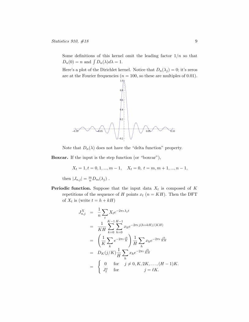
Some definitions of this kernel omit the leading factor 1/n so thatDn(0) = n and

∫Dn(λ)dλ = 1.

Here’s a plot of the Dirichlet kernel. Notice that Dn(λj) = 0; it’s zerosare at the Fourier frequencies (n = 100, so these are multiples of 0.01).

-0.10 -0.05 0.05 0.10

-0.2

0.2

0.4

0.6

0.8

1.0

Note that Dn(λ) does not have the “delta function” property.

Boxcar. If the input is the step function (or “boxcar”),

Xt = 1, t = 0, 1, ...,m− 1, Xt = 0, t = m,m+ 1, ..., n− 1,

then |Jn,j | = mnDm(λj) .

Periodic function. Suppose that the input data Xt is composed of Krepetitions of the sequence of H points xt (n = KH). Then the DFTof Xt is (write t = h+ kH)

JXn,j =1n

∑t

Xte−2πı λjt

=1

KH

K−1∑k=0

H−1∑h=0

xhe−2πı j(h+kH)/(KH)

=

(1K

∑k

e−2πı jkK

)1H

∑h

xhe−2πı jh

KH

= DK(j/K)1H

∑h

xhe−2πı jh

KH

=

{0 for j 6= 0,K, 2K, . . . , (H − 1)K.Jx` for j = `K.

Statistics 910, #18 10

The transform of the y’s is zero except at multiples of K/n, which isknown as the fundamental frequency.

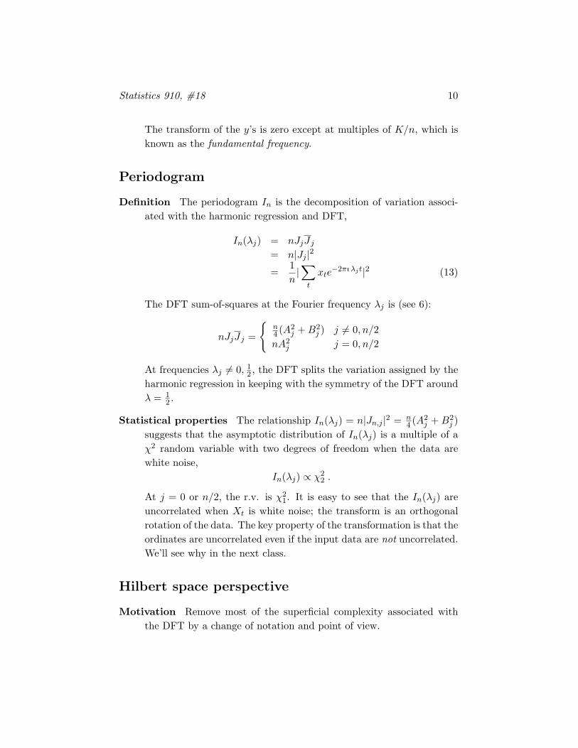
Periodogram

Definition The periodogram In is the decomposition of variation associ-ated with the harmonic regression and DFT,

In(λj) = nJjJ j= n|Jj |2

=1n|∑t

xte−2πı λjt|2 (13)

The DFT sum-of-squares at the Fourier frequency λj is (see 6):

nJjJ j =

{n4 (A2

j +B2j ) j 6= 0, n/2

nA2j j = 0, n/2

At frequencies λj 6= 0, 12 , the DFT splits the variation assigned by the

harmonic regression in keeping with the symmetry of the DFT aroundλ = 1

2 .

Statistical properties The relationship In(λj) = n|Jn,j |2 = n4 (A2

j + B2j )

suggests that the asymptotic distribution of In(λj) is a multiple of aχ2 random variable with two degrees of freedom when the data arewhite noise,

In(λj) ∝ χ22 .

At j = 0 or n/2, the r.v. is χ21. It is easy to see that the In(λj) are

uncorrelated when Xt is white noise; the transform is an orthogonalrotation of the data. The key property of the transformation is that theordinates are uncorrelated even if the input data are not uncorrelated.We’ll see why in the next class.

Hilbert space perspective

Motivation Remove most of the superficial complexity associated withthe DFT by a change of notation and point of view.

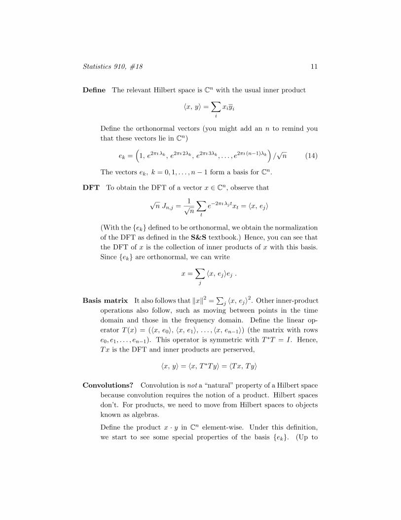
Statistics 910, #18 11

Define The relevant Hilbert space is Cn with the usual inner product

〈x, y〉 =∑i

xiyi

Define the orthonormal vectors (you might add an n to remind youthat these vectors lie in Cn)

ek =(

1, e2πı λk , e2πı 2λk , e2πı 3λk , . . . , e2πı (n−1)λk

)/√n (14)

The vectors ek, k = 0, 1, . . . , n− 1 form a basis for Cn.

DFT To obtain the DFT of a vector x ∈ Cn, observe that

√n Jn,j =

1√n

∑t

e−2πı λjtxt = 〈x, ej〉

(With the {ek} defined to be orthonormal, we obtain the normalizationof the DFT as defined in the S&S textbook.) Hence, you can see thatthe DFT of x is the collection of inner products of x with this basis.Since {ek} are orthonormal, we can write

x =∑j

〈x, ej〉ej .

Basis matrix It also follows that ‖x‖2 =∑

j 〈x, ej〉2. Other inner-product

operations also follow, such as moving between points in the timedomain and those in the frequency domain. Define the linear op-erator T (x) = (〈x, e0〉, 〈x, e1〉, . . . , 〈x, en−1〉) (the matrix with rowse0, e1, . . . , en−1). This operator is symmetric with T ∗T = I. Hence,Tx is the DFT and inner products are perserved,

〈x, y〉 = 〈x, T ∗Ty〉 = 〈Tx, Ty〉

Convolutions? Convolution is not a “natural” property of a Hilbert spacebecause convolution requires the notion of a product. Hilbert spacesdon’t. For products, we need to move from Hilbert spaces to objectsknown as algebras.

Define the product x · y in Cn element-wise. Under this definition,we start to see some special properties of the basis {ek}. (Up to

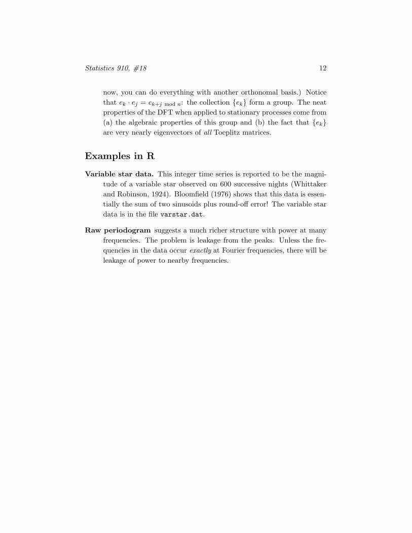
Statistics 910, #18 12

now, you can do everything with another orthonomal basis.) Noticethat ek · ej = ek+j mod n: the collection {ek} form a group. The neatproperties of the DFT when applied to stationary processes come from(a) the algebraic properties of this group and (b) the fact that {ek}are very nearly eigenvectors of all Toeplitz matrices.

Examples in R

Variable star data. This integer time series is reported to be the magni-tude of a variable star observed on 600 successive nights (Whittakerand Robinson, 1924). Bloomfield (1976) shows that this data is essen-tially the sum of two sinusoids plus round-off error! The variable stardata is in the file varstar.dat.

Raw periodogram suggests a much richer structure with power at manyfrequencies. The problem is leakage from the peaks. Unless the fre-quencies in the data occur exactly at Fourier frequencies, there will beleakage of power to nearby frequencies.