Differential Analysis Lecture notes for 18.155 and 156 Richard B. Melrose
243
Differential Analysis Lecture notes for 18.155 and 156 Richard B. Melrose
Transcript of Differential Analysis Lecture notes for 18.155 and 156 Richard B. Melrose
Differential Analysis
Lecture notes for 18.155 and 156
Richard B. Melrose

Contents
Introduction 6
Chapter 1. Measure and Integration 71. Continuous functions 72. Measures and σ-algebras 143. Measureability of functions 204. Integration 22
Chapter 2. Hilbert spaces and operators 351. Hilbert space 352. Spectral theorem 38
Chapter 3. Distributions 431. Test functions 432. Tempered distributions 503. Convolution and density 554. Fourier inversion 655. Sobolev embedding 706. Differential operators. 747. Cone support and wavefront set 898. Homogeneous distributions 1029. Operators and kernels 10310. Fourier transform 10311. Schwartz space. 10312. Tempered distributions. 10413. Fourier transform 10514. Sobolev spaces 10615. Weighted Sobolev spaces. 10916. Multiplicativity 11217. Some bounded operators 115
Chapter 4. Elliptic Regularity 1171. Constant coefficient operators 1172. Constant coefficient elliptic operators 1193. Interior elliptic estimates 126
3
4 CONTENTS
Addenda to Chapter 4 135
Chapter 5. Coordinate invariance and manifolds 1371. Local diffeomorphisms 1372. Manifolds 1413. Vector bundles 147
Chapter 6. Invertibility of elliptic operators 1491. Global elliptic estimates 1492. Compact inclusion of Sobolev spaces 1523. Elliptic operators are Fredholm 1534. Generalized inverses 1575. Self-adjoint elliptic operators 1606. Index theorem 165Addenda to Chapter 6 165
Chapter 7. Suspended families and the resolvent 1671. Product with a line 1672. Translation-invariant Operators 1743. Invertibility 1804. Resolvent operator 185Addenda to Chapter 7 185
Chapter 8. Manifolds with boundary 1871. Compactifications of R. 1872. Basic properties 1913. Boundary Sobolev spaces 1924. Dirac operators 1925. Homogeneous translation-invariant operators 1926. Scattering structure 195
Chapter 9. Electromagnetism 2011. Maxwell’s equations 2012. Hodge Theory 2043. Coulomb potential 2084. Dirac strings 208Addenda to Chapter 9 208
Chapter 10. Monopoles 2091. Gauge theory 2092. Bogomolny equations 2093. Problems 2094. Solutions to (some of) the problems 236

CONTENTS 5
Bibliography 243
6 CONTENTS
Introduction
These notes are for the graduate analysis courses (18.155 and 18.156)at MIT. They are based on various earlier similar courses. In givingthe lectures I usually cut many corners!
To thank:- Austin Frakt, Philip Dorrell, Jacob Bernstein....

CHAPTER 1
Measure and Integration
A rather quick review of measure and integration.
1. Continuous functions
A the beginning I want to remind you of things I think you alreadyknow and then go on to show the direction the course will be taking.Let me first try to set the context.
One basic notion I assume you are reasonably familiar with is thatof a metric space ([6] p.9). This consists of a set, X, and a distancefunction
d : X ×X = X2 −→ [0,∞) ,
satisfying the following three axioms:
(1.1)
i) d(x, y) = 0⇔ x = y, (and d(x, y) ≥ 0)
ii) d(x, y) = d(y, x) ∀ x, y ∈ Xiii) d(x, y) ≤ d(x, z) + d(z, y) ∀ x, y, z ∈ X.
The basic theory of metric spaces deals with properties of subsets(open, closed, compact, connected), sequences (convergent, Cauchy)and maps (continuous) and the relationship between these notions.Let me just remind you of one such result.
Proposition 1.1. A map f : X → Y between metric spaces iscontinuous if and only if one of the three following equivalent conditionsholds
(1) f−1(O) ⊂ X is open ∀ O ⊂ Y open.(2) f−1(C) ⊂ X is closed ∀ C ⊂ Y closed.(3) limn→∞ f(xn) = f(x) in Y if xn → x in X.
The basic example of a metric space is Euclidean space. Real n-dimensional Euclidean space, Rn, is the set of ordered n-tuples of realnumbers
x = (x1, . . . , xn) ∈ Rn , xj ∈ R , j = 1, . . . , n .
7
8 1. MEASURE AND INTEGRATION
It is also the basic example of a vector (or linear) space with the oper-ations
x+ y = (x1 + y1, x2 + y2, . . . , xn + yn)
cx = (cx1, . . . , cxn) .
The metric is usually taken to be given by the Euclidean metric
|x| = (x21 + · · ·+ x2
n)1/2 = (n∑j=1
x2j)
1/2 ,
in the sense thatd(x, y) = |x− y| .
Let us abstract this immediately to the notion of a normed vectorspace, or normed space. This is a vector space V (over R or C) equippedwith a norm, which is to say a function
‖ ‖ : V −→ [0,∞)
satisfying
(1.2)
i) ‖v‖ = 0⇐⇒ v = 0,
ii) ‖cv‖ = |c| ‖v‖ ∀ c ∈ K,iii) ‖v + w‖ ≤ ‖v‖+ ‖w‖.
This means that (V, d), d(v, w) = ‖v − w‖ is a vector space; I am alsousing K to denote either R or C as is appropriate.
The case of a finite dimensional normed space is not very interestingbecause, apart from the dimension, they are all “the same”. We shallsay (in general) that two norms ‖ • ‖1 and ‖ • ‖2 on V are equivalentof there exists C > 0 such that
1
C‖v‖1 ≤ ‖v‖2 ≤ C‖v‖1 ∀ v ∈ V .
Proposition 1.2. Any two norms on a finite dimensional vectorspace are equivalent.
So, we are mainly interested in the infinite dimensional case. I willstart the course, in a slightly unorthodox manner, by concentrating onone such normed space (really one class). Let X be a metric space.The case of a continuous function, f : X → R (or C) is a special caseof Proposition 1.1 above. We then define
C(X) = f : X → R, f bounded and continuous .In fact the same notation is generally used for the space of complex-
valued functions. If we want to distinguish between these two possi-bilities we can use the more pedantic notation C(X;R) and C(X;C).
1. CONTINUOUS FUNCTIONS 9
Now, the ‘obvious’ norm on this linear space is the supremum (or ‘uni-form’) norm
‖f‖∞ = supx∈X|f(x)| .
Here X is an arbitrary metric space. For the moment X is sup-posed to be a “physical” space, something like Rn. Corresponding tothe finite-dimensionality of Rn we often assume (or demand) that Xis locally compact. This just means that every point has a compactneighborhood, i.e., is in the interior of a compact set. Whether locallycompact or not we can consider
(1.3) C0(X) =
f ∈ C(X); ∀ ε > 0 ∃ K b Xs.t. sup
x/∈K|f(x)| ≤ ε
.
Here the notation K b X means ‘K is a compact subset of X’.If V is a normed linear space we are particularly interested in the
continuous linear functionals on V . Here ‘functional’ just means func-tion but V is allowed to be ‘large’ (not like Rn) so ‘functional’ is usedfor historical reasons.
Proposition 1.3. The following are equivalent conditions on alinear functional u : V −→ R on a normed space V .
(1) u is continuous.(2) u is continuous at 0.(3) u(f) ∈ R ; f ∈ V , ‖f‖ ≤ 1 is bounded.(4) ∃ C s.t. |u(f)| ≤ C‖f‖ ∀ f ∈ V .
Proof. (1) =⇒ (2) by definition. Then (2) implies that u−1(−1, 1)is a neighborhood of 0 ∈ V , so for some ε > 0, u(f ∈ V ; ‖f‖ < ε) ⊂(−1, 1). By linearity of u, u(f ∈ V ; ‖f‖ < 1) ⊂ (−1
ε, 1ε) is bounded,
so (2) =⇒ (3). Then (3) implies that
|u(f)| ≤ C ∀ f ∈ V, ‖f‖ ≤ 1
for some C. Again using linearity of u, if f 6= 0,
|u(f)| ≤ ‖f‖u(
f
‖f‖
)≤ C‖f‖ ,
giving (4). Finally, assuming (4),
|u(f)− u(g)| = |u(f − g)| ≤ C‖f − g‖shows that u is continuous at any point g ∈ V .
In view of this identification, continuous linear functionals are oftensaid to be bounded. One of the important ideas that we shall exploitlater is that of ‘duality’. In particular this suggests that it is a good
10 1. MEASURE AND INTEGRATION
idea to examine the totality of bounded linear functionals on V . Thedual space is
V ′ = V ∗ = u : V −→ K , linear and bounded .
This is also a normed linear space where the linear operations are
(1.4)(u+ v)(f) = u(f) + v(f)
(cu)(f) = c(u(f))∀ f ∈ V.
The natural norm on V ′ is
‖u‖ = sup‖f‖≤1
|u(f)|.
This is just the ‘best constant’ in the boundedness estimate,
‖u‖ = inf C; |u(f)| ≤ C‖f‖ ∀ f ⊂ V .
One of the basic questions I wish to pursue in the first part of thecourse is: What is the dual of C0(X) for a locally compact metric spaceX? The answer is given by Riesz’ representation theorem, in terms of(Borel) measures.
Let me give you a vague picture of ‘regularity of functions’ whichis what this course is about, even though I have not introduced mostof these spaces yet. Smooth functions (and small spaces) are towardsthe top. Duality flips up and down and as we shall see L2, the spaceof Lebesgue square-integrable functions, is generally ‘in the middle’.What I will discuss first is the right side of the diagramme, where wehave the space of continuous functions on Rn which vanish at infinityand its dual space, Mfin(Rn), the space of finite Borel measures. Thereare many other spaces that you may encounter, here I only include testfunctions, Schwartz functions, Sobolev spaces and their duals; k is a
1. CONTINUOUS FUNCTIONS 11
general positive integer.
(1.5) S(Rn) _
w
**Hk(Rn)
_
Cc(Rn) //
_
kK
yy
C0(Rn)
L2(Rb) _
s
%%H−k(Rn)
_
M(Rn) Mfin(Rn)gG
tt
? _oo
S ′(Rn).
I have set the goal of understanding the dual space Mfin(Rn) ofC0(X), where X is a locally compact metric space. This will force meto go through the elements of measure theory and Lebesgue integration.It does require a little forcing!
The basic case of interest is Rn. Then an obvious example of acontinuous linear functional on C0(Rn) is given by Riemann integration,for instance over the unit cube [0, 1]n:
u(f) =
∫[0,1]n
f(x) dx .
In some sense we must show that all continuous linear functionalson C0(X) are given by integration. However, we have to interpretintegration somewhat widely since there are also evaluation functionals.If z ∈ X consider the Dirac delta
δz(f) = f(z) .
This is also called a point mass of z. So we need a theory of measureand integration wide enough to include both of these cases.
One special feature of C0(X), compared to general normed spaces,is that there is a notion of positivity for its elements. Thus f ≥ 0 justmeans f(x) ≥ 0 ∀ x ∈ X.
Lemma 1.4. Each f ∈ C0(X) can be decomposed uniquely as thedifference of its positive and negative parts
(1.6) f = f+ − f− , f± ∈ C0(X) , f±(x) ≤ |f(x)| ∀ x ∈ X .
12 1. MEASURE AND INTEGRATION
Proof. Simply define
f±(x) =
±f(x) if ±f(x) ≥ 0
0 if ±f(x) < 0
for the same sign throughout. Then (3.8) holds. Observe that f+ iscontinuous at each y ∈ X since, with U an appropriate neighborhoodof y, in each case
f(y) > 0 =⇒ f(x) > 0 for x ∈ U =⇒ f+ = f in U
f(y) < 0 =⇒ f(x) < 0 for x ∈ U =⇒ f+ = 0 in U
f(y) = 0 =⇒ given ε > 0 ∃ U s.t. |f(x)| < ε in U
=⇒ |f+(x)| < ε in U .
Thus f− = f−f+ ∈ C0(X), since both f+ and f− vanish at infinity.
We can similarly split elements of the dual space into positive andnegative parts although it is a little bit more delicate. We say thatu ∈ (C0(X))′ is positive if
(1.7) u(f) ≥ 0 ∀ 0 ≤ f ∈ C0(X) .
For a general (real) u ∈ (C0(X))′ and for each 0 ≤ f ∈ C0(X) set
(1.8) u+(f) = sup u(g) ; g ∈ C0(X) , 0 ≤ g(x) ≤ f(x) ∀ x ∈ X .This is certainly finite since u(g) ≤ C‖g‖∞ ≤ C‖f‖∞. Moreover, if0 < c ∈ R then u+(cf) = cu+(f) by inspection. Suppose 0 ≤ fi ∈C0(X) for i = 1, 2. Then given ε > 0 there exist gi ∈ C0(X) with0 ≤ gi(x) ≤ fi(x) and
u+(fi) ≤ u(gi) + ε .
It follows that 0 ≤ g(x) ≤ f1(x) + f2(x) if g = g1 + g2 so
u+(f1 + f2) ≥ u(g) = u(g1) + u(g2) ≥ u+(f1) + u+(f2)− 2ε .
Thusu+(f1 + f2) ≥ u+(f1) + u+(f2).
Conversely, if 0 ≤ g(x) ≤ f1(x) + f2(x) set g1(x) = min(g, f1) ∈C0(X) and g2 = g − g1. Then 0 ≤ gi ≤ fi and u+(f1) + u+(f2) ≥u(g1) + u(g2) = u(g). Taking the supremum over g, u+(f1 + f2) ≤u+(f1) + u+(f2), so we find
(1.9) u+(f1 + f2) = u+(f1) + u+(f2) .
Having shown this effective linearity on the positive functions wecan obtain a linear functional by setting
(1.10) u+(f) = u+(f+)− u+(f−) ∀ f ∈ C0(X) .
1. CONTINUOUS FUNCTIONS 13
Note that (1.9) shows that u+(f) = u+(f1) − u+(f2) for any decom-posiiton of f = f1−f2 with fi ∈ C0(X), both positive. [Since f1 +f− =f2 + f+ so u+(f1) + u+(f−) = u+(f2) + u+(f+).] Moreover,
|u+(f)| ≤ max(u+(f+), u(f−)) ≤ ‖u‖ ‖f‖∞=⇒ ‖u+‖ ≤ ‖u‖ .
The functionalu− = u+ − u
is also positive, since u+(f) ≥ u(f) for all 0 ≤ f ∈ C0(x). Thus wehave proved
Lemma 1.5. Any element u ∈ (C0(X))′ can be decomposed,
u = u+ − u−into the difference of positive elements with
‖u+‖ , ‖u−‖ ≤ ‖u‖ .
The idea behind the definition of u+ is that u itself is, more orless, “integration against a function” (even though we do not knowhow to interpret this yet). In defining u+ from u we are effectivelythrowing away the negative part of that ‘function.’ The next step isto show that a positive functional corresponds to a ‘measure’ meaninga function measuring the size of sets. To define this we really want toevaluate u on the characteristic function of a set
χE(x) =
1 if x ∈ E0 if x /∈ E .
The problem is that χE is not continuous. Instead we use an ideasimilar to (15.9).
If 0 ≤ u ∈ (C0(X))′ and U ⊂ X is open, set1
(1.11) µ(U) = sup u(f) ; 0 ≤ f(x) ≤ 1, f ∈ C0(X) , supp(f) b U .Here the support of f , supp(f), is the closure of the set of points wheref(x) 6= 0. Thus supp(f) is always closed, in (15.4) we only admit f ifits support is a compact subset of U. The reason for this is that, onlythen do we ‘really know’ that f ∈ C0(X).
Suppose we try to measure general sets in this way. We can do thisby defining
(1.12) µ∗(E) = inf µ(U) ; U ⊃ E , U open .Already with µ it may happen that µ(U) =∞, so we think of
(1.13) µ∗ : P(X)→ [0,∞]
1See [6] starting p.42 or [1] starting p.206.
14 1. MEASURE AND INTEGRATION
as defined on the power set of X and taking values in the extendedpositive real numbers.
Definition 1.6. A positive extended function, µ∗, defined on thepower set of X is called an outer measure if µ∗(∅) = 0, µ∗(A) ≤ µ∗(B)whenever A ⊂ B and
(1.14) µ∗(⋃j
Aj) ≤∑j
µ(Aj) ∀ Aj∞j=1 ⊂ P(X) .
Lemma 1.7. If u is a positive continuous linear functional on C0(X)then µ∗, defined by (15.4), (15.12) is an outer measure.
To prove this we need to find enough continuous functions. I haverelegated the proof of the following result to Problem 2.
Lemma 1.8. Suppose Ui, i = 1, . . . , N is ,a finite collection of opensets in a locally compact metric space and K b
⋃Ni=1 Ui is a compact
subset, then there exist continuous functions fi ∈ C(X) with 0 ≤ fi ≤1, supp(fi) b Ui and
(1.15)∑i
fi = 1 in a neighborhood of K .
Proof of Lemma 15.8. We have to prove (15.6). Suppose firstthat the Ai are open, then so is A =
⋃iAi. If f ∈ C(X) and
supp(f) b A then supp(f) is covered by a finite union of the Ais.Applying Lemma 15.7 we can find fi’s, all but a finite number iden-tically zero, so supp(fi) b Ai and
∑i fi = 1 in a neighborhood of
supp(f).Since f =
∑i fif we conclude that
u(f) =∑i
u(fif) =⇒ µ∗(A) ≤∑i
µ∗(Ai)
since 0 ≤ fif ≤ 1 and supp(fif) b Ai.Thus (15.6) holds when the Ai are open. In the general case if
Ai ⊂ Bi with the Bi open then, from the definition,
µ∗(⋃i
Ai) ≤ µ∗(⋃i
Bi) ≤∑i
µ∗(Bi) .
Taking the infimum over the Bi gives (15.6) in general.
2. Measures and σ-algebras
An outer measure such as µ∗ is a rather crude object since, evenif the Ai are disjoint, there is generally strict inequality in (15.6). Itturns out to be unreasonable to expect equality in (15.6), for disjoint
2. MEASURES AND σ-ALGEBRAS 15
unions, for a function defined on all subsets of X. We therefore restrictattention to smaller collections of subsets.
Definition 2.1. A collection of subsetsM of a set X is a σ-algebraif
(1) φ,X ∈M(2) E ∈M =⇒ EC = X\E ∈M(3) Ei∞i=1 ⊂M =⇒
⋃∞i=1 Ei ∈M.
For a general outer measure µ∗ we define the notion of µ∗-measurabilityof a set.
Definition 2.2. A set E ⊂ X is µ∗-measurable (for an outer mea-sure µ∗ on X) if
(2.1) µ∗(A) = µ∗(A ∩ E) + µ∗(A ∩ E) ∀ A ⊂ X .
Proposition 2.3. The collection of µ∗-measurable sets for anyouter measure is a σ-algebra.
Proof. Suppose E is µ∗-measurable, then EC is µ∗-measurable bythe symmetry of (3.9).
Suppose A, E and F are any three sets. Then
A ∩ (E ∪ F ) = (A ∩ E ∩ F ) ∪ (A ∩ E ∩ FC) ∪ (A ∩ EC ∩ F )
A ∩ (E ∪ F )C = A ∩ EC ∩ FC .
From the subadditivity of µ∗
µ∗(A ∩ (E ∪ F )) + µ∗(A ∩ (E ∪ F )C)
≤ µ∗(A ∩ E ∩ F ) + µ∗(A ∩ E ∪ FC)
+ µ∗(A ∩ EC ∩ F ) + µ∗(A ∩ EC ∩ FC).
Now, if E and F are µ∗-measurable then applying the definition twice,for any A,
µ∗(A) = µ∗(A ∩ E ∩ F ) + µ∗(A ∩ E ∩ FC)
+ µ∗(A ∩ EC ∩ F ) + µ∗(A ∩ EC ∩ FC)
≥ µ∗(A ∩ (E ∪ F )) + µ∗(A ∩ (E ∪ F )C) .
The reverse inequality follows from the subadditivity of µ∗, so E ∪ Fis also µ∗-measurable.
If Ei∞i=1 is a sequence of disjoint µ∗-measurable sets, set Fn =⋃ni=1 Ei and F =
⋃∞i=1Ei. Then for any A,
µ∗(A ∩ Fn) = µ∗(A ∩ Fn ∩ En) + µ∗(A ∩ Fn ∩ ECn )
= µ∗(A ∩ En) + µ∗(A ∩ Fn−1) .
16 1. MEASURE AND INTEGRATION
Iterating this shows that
µ∗(A ∩ Fn) =n∑j=1
µ∗(A ∩ Ej) .
From the µ∗-measurability of Fn and the subadditivity of µ∗,
µ∗(A) = µ∗(A ∩ Fn) + µ∗(A ∩ FCn )
≥n∑j=1
µ∗(A ∩ Ej) + µ∗(A ∩ FC) .
Taking the limit as n→∞ and using subadditivity,
µ∗(A) ≥∞∑j=1
µ∗(A ∩ Ej) + µ∗(A ∩ FC)(2.2)
≥ µ∗(A ∩ F ) + µ∗(A ∩ FC) ≥ µ∗(A)
proves that inequalities are equalities, so F is also µ∗-measurable.In general, for any countable union of µ∗-measurable sets,
∞⋃j=1
Aj =∞⋃j=1
Aj ,
Aj = Aj\j−1⋃i=1
Ai = Aj ∩
(j−1⋃i=1
Ai
)C
is µ∗-measurable since the Aj are disjoint.
A measure (sometimes called a positive measure) is an extendedfunction defined on the elements of a σ-algebra M:
µ :M→ [0,∞]
such that
µ(∅) = 0 and(2.3)
µ
(∞⋃i=1
Ai
)=∞∑i=1
µ(Ai)
if Ai∞i=1 ⊂M and Ai ∩ Aj = φ i 6= j.
(2.4)
The elements of M with measure zero, i.e., E ∈ M, µ(E) = 0, aresupposed to be ‘ignorable’. The measure µ is said to be complete if
(2.5) E ⊂ X and ∃ F ∈M , µ(F ) = 0 , E ⊂ F ⇒ E ∈M .
See Problem 4.
2. MEASURES AND σ-ALGEBRAS 17
The first part of the following important result due to Caratheodorywas shown above.
Theorem 2.4. If µ∗ is an outer measure on X then the collectionof µ∗-measurable subsets of X is a σ-algebra and µ∗ restricted to M isa complete measure.
Proof. We have already shown that the collection of µ∗-measurablesubsets of X is a σ-algebra. To see the second part, observe that takingA = F in (3.11) gives
µ∗(F ) =∑j
µ∗(Ej) if F =∞⋃j=1
Ej
and the Ej are disjoint elements of M. This is (3.3).Similarly if µ∗(E) = 0 and F ⊂ E then µ∗(F ) = 0. Thus it is
enough to show that for any subset E ⊂ X, µ∗(E) = 0 implies E ∈M.For any A ⊂ X, using the fact that µ∗(A∩E) = 0, and the ‘increasing’property of µ∗
µ∗(A) ≤ µ∗(A ∩ E) + µ∗(A ∩ EC)
= µ∗(A ∩ EC) ≤ µ∗(A)
shows that these must always be equalities, so E ∈ M (i.e., is µ∗-measurable).
Going back to our primary concern, recall that we constructed theouter measure µ∗ from 0 ≤ u ∈ (C0(X))′ using (15.4) and (15.12). Forthe measure whose existence follows from Caratheodory’s theorem tobe much use we need
Proposition 2.5. If 0 ≤ u ∈ (C0(X))′, for X a locally compactmetric space, then each open subset of X is µ∗-measurable for the outermeasure defined by (15.4) and (15.12) and µ in (15.4) is its measure.
Proof. Let U ⊂ X be open. We only need to prove (3.9) for allA ⊂ X with µ∗(A) <∞.2
Suppose first that A ⊂ X is open and µ∗(A) < ∞. Then A ∩ Uis open, so given ε > 0 there exists f ∈ C(X) supp(f) b A ∩ U with0 ≤ f ≤ 1 and
µ∗(A ∩ U) = µ(A ∩ U) ≤ u(f) + ε .
Now, A\ supp(f) is also open, so we can find g ∈ C(X) , 0 ≤ g ≤1 , supp(g) b A\ supp(f) with
µ∗(A\ supp(f)) = µ(A\ supp(f)) ≤ u(g) + ε .
2Why?
18 1. MEASURE AND INTEGRATION
Since
A\ supp(f) ⊃ A ∩ UC , 0 ≤ f + g ≤ 1 , supp(f + g) b A ,
µ(A) ≥ u(f + g) = u(f) + u(g)
> µ∗(A ∩ U) + µ∗(A ∩ UC)− 2ε
≥ µ∗(A)− 2ε
using subadditivity of µ∗. Letting ε ↓ 0 we conclude that
µ∗(A) ≤ µ∗(A ∩ U) + µ∗(A ∩ UC) ≤ µ∗(A) = µ(A) .
This gives (3.9) when A is open.In general, if E ⊂ X and µ∗(E) <∞ then given ε > 0 there exists
A ⊂ X open with µ∗(E) > µ∗(A)− ε. Thus,
µ∗(E) ≥ µ∗(A ∩ U) + µ∗(A ∩ UC)− ε≥ µ∗(E ∩ U) + µ∗(E ∩ UC)− ε≥ µ∗(E)− ε .
This shows that (3.9) always holds, so U is µ∗-measurable if it is open.We have already observed that µ(U) = µ∗(U) if U is open.
Thus we have shown that the σ-algebra given by Caratheodory’stheorem contains all open sets. You showed in Problem 3 that theintersection of any collection of σ-algebras on a given set is a σ-algebra.Since P(X) is always a σ-algebra it follows that for any collectionE ⊂ P(X) there is always a smallest σ-algebra containing E , namely
ME =⋂M ⊃ E ; M is a σ-algebra ,M⊂ P(X) .
The elements of the smallest σ-algebra containing the open sets arecalled ‘Borel sets’. A measure defined on the σ-algebra of all Borel setsis called a Borel measure. This we have shown:
Proposition 2.6. The measure defined by (15.4), (15.12) from0 ≤ u ∈ (C0(X))′ by Caratheodory’s theorem is a Borel measure.
Proof. This is what Proposition 3.14 says! See how easy proofsare.
We can even continue in the same vein. A Borel measure is said tobe outer regular on E ⊂ X if
(2.6) µ(E) = inf µ(U) ; U ⊃ E , U open .Thus the measure constructed in Proposition 3.14 is outer regular onall Borel sets! A Borel measure is inner regular on E if
(2.7) µ(E) = sup µ(K) ; K ⊂ E , K compact .
2. MEASURES AND σ-ALGEBRAS 19
Here we need to know that compact sets are Borel measurable. Thisis Problem 5.
Definition 2.7. A Radon measure (on a metric space) is a Borelmeasure which is outer regular on all Borel sets, inner regular on opensets and finite on compact sets.
Proposition 2.8. The measure defined by (15.4), (15.12) from0 ≤ u ∈ (C0(X))′ using Caratheodory’s theorem is a Radon measure.
Proof. Suppose K ⊂ X is compact. Let χK be the charac-teristic function of K , χK = 1 on K , χK = 0 on KC . Supposef ∈ C0(X) , supp(f) b X and f ≥ χK . Set
Uε = x ∈ X ; f(x) > 1− ε
where ε > 0 is small. Thus Uε is open, by the continuity of f andcontains K. Moreover, we can choose g ∈ C(X) , supp(g) b Uε , 0 ≤g ≤ 1 with g = 1 near3 K. Thus, g ≤ (1− ε)−1f and hence
µ∗(K) ≤ u(g) = (1− ε)−1u(f) .
Letting ε ↓ 0, and using the measurability of K,
µ(K) ≤ u(f)
⇒ µ(K) = inf u(f) ; f ∈ C(X) , supp(f) b X , f ≥ χK .
In particular this implies that µ(K) <∞ if K b X, but is also proves(3.17).
Let me now review a little of what we have done. We used thepositive functional u to define an outer measure µ∗, hence a measureµ and then checked the properties of the latter.
This is a pretty nice scheme; getting ahead of myself a little, let mesuggest that we try it on something else.
Let us say that Q ⊂ Rn is ‘rectangular’ if it is a product of finiteintervals (open, closed or half-open)
(2.8) Q =n∏i=1
(or[ai , bi]or) ai ≤ bi
we all agree on its standard volume:
(2.9) v(Q) =n∏i=1
(bi − ai) ∈ [0,∞) .
3Meaning in a neighborhood of K.
20 1. MEASURE AND INTEGRATION
Clearly if we have two such sets, Q1 ⊂ Q2, then v(Q1) ≤ v(Q2). Letus try to define an outer measure on subsets of Rn by
(2.10) v∗(A) = inf
∞∑i=1
v(Qi) ; A ⊂∞⋃i=1
Qi, Qi rectangular
.
We want to show that (3.22) does define an outer measure. This ispretty easy; certainly v(∅) = 0. Similarly if Ai∞i=1 are (disjoint) setsand Qij∞i=1 is a covering of Ai by open rectangles then all the Qij
together cover A =⋃iAi and
v∗(A) ≤∑i
∑j
v(Qij)
⇒ v∗(A) ≤∑i
v∗(Ai) .
So we have an outer measure. We also want
Lemma 2.9. If Q is rectangular then v∗(Q) = v(Q).
Assuming this, the measure defined from v∗ using Caratheodory’stheorem is called Lebesgue measure.
Proposition 2.10. Lebesgue measure is a Borel measure.
To prove this we just need to show that (open) rectangular sets arev∗-measurable.
3. Measureability of functions
Suppose thatM is a σ-algebra on a set X4 and N is a σ-algebra onanother set Y. A map f : X → Y is said to be measurable with respectto these given σ-algebras on X and Y if
(3.1) f−1(E) ∈M ∀ E ∈ N .
Notice how similar this is to one of the characterizations of continuityfor maps between metric spaces in terms of open sets. Indeed thisanalogy yields a useful result.
Lemma 3.1. If G ⊂ N generates N , in the sense that
(3.2) N =⋂N ′;N ′ ⊃ G, N ′ a σ-algebra
then f : X −→ Y is measurable iff f−1(A) ∈M for all A ∈ G.
4Then X, or if you want to be pedantic (X,M), is often said to be a measurespace or even a measurable space.
3. MEASUREABILITY OF FUNCTIONS 21
Proof. The main point to note here is that f−1 as a map on powersets, is very well behaved for any map. That is if f : X → Y thenf−1 : P(Y )→ P(X) satisfies:
(3.3)
f−1(EC) = (f−1(E))C
f−1
(∞⋃j=1
Ej
)=∞⋃j=1
f−1(Ej)
f−1
(∞⋂j=1
Ej
)=∞⋂j=1
f−1(Ej)
f−1(φ) = φ , f−1(Y ) = X .
Putting these things together one sees that if M is any σ-algebra onX then
(3.4) f∗(M) =E ⊂ Y ; f−1(E) ∈M
is always a σ-algebra on Y.
In particular if f−1(A) ∈M for all A ∈ G ⊂ N then f∗(M) is a σ-algebra containing G, hence containing N by the generating condition.Thus f−1(E) ∈M for all E ∈ N so f is measurable.
Proposition 3.2. Any continuous map f : X → Y between metricspaces is measurable with respect to the Borel σ-algebras on X and Y.
Proof. The continuity of f shows that f−1(E) ⊂ X is open if E ⊂Y is open. By definition, the open sets generate the Borel σ-algebraon Y so the preceeding Lemma shows that f is Borel measurable i.e.,
f−1(B(Y )) ⊂ B(X).
We are mainly interested in functions on X. If M is a σ-algebraon X then f : X → R is measurable if it is measurable with respectto the Borel σ-algebra on R and M on X. More generally, for anextended function f : X → [−∞,∞] we take as the ‘Borel’ σ-algebrain [−∞,∞] the smallest σ-algebra containing all open subsets of R andall sets (a,∞] and [−∞, b); in fact it is generated by the sets (a,∞].(See Problem 6.)
Our main task is to define the integral of a measurable function: westart with simple functions. Observe that the characteristic functionof a set
χE =
1 x ∈ E0 x /∈ E
22 1. MEASURE AND INTEGRATION
is measurable if and only if E ∈M. More generally a simple function,
(3.5) f =N∑i=1
aiχEi , ai ∈ R
is measurable if the Ei are measurable. The presentation, (3.5), of asimple function is not unique. We can make it so, getting the minimalpresentation, by insisting that all the ai are non-zero and
Ei = x ∈ E ; f(x) = ai
then f in (3.5) is measurable iff all the Ei are measurable.The Lebesgue integral is based on approximation of functions by
simple functions, so it is important to show that this is possible.
Proposition 3.3. For any non-negative µ-measurable extended func-tion f : X −→ [0,∞] there is an increasing sequence fn of simple mea-surable functions such that limn→∞ fn(x) = f(x) for each x ∈ X andthis limit is uniform on any measurable set on which f is finite.
Proof. Folland [1] page 45 has a nice proof. For each integer n > 0and 0 ≤ k ≤ 22n − 1, set
En,k = x ∈ X; 2−nk ≤ f(x) < 2−n(k + 1),E ′n = x ∈ X; f(x) ≥ 2n.
These are measurable sets. On increasing n by one, the interval in thedefinition of En,k is divided into two. It follows that the sequence ofsimple functions
(3.6) fn =∑k
2−nkχEk,n + 2nχE′n
is increasing and has limit f and that this limit is uniform on anymeasurable set where f is finite.
4. Integration
The (µ)-integral of a non-negative simple function is by definition
(4.1)
∫Y
f dµ =∑i
aiµ(Y ∩ Ei) , Y ∈M .
Here the convention is that if µ(Y ∩Ei) =∞ but ai = 0 then ai ·µ(Y ∩Ei) = 0. Clearly this integral takes values in [0,∞]. More significantly,
4. INTEGRATION 23
if c ≥ 0 is a constant and f and g are two non-negative (µ-measurable)simple functions then
(4.2)
∫Y
cfdµ = c
∫Y
fdµ∫Y
(f + g)dµ =
∫Y
fdµ+
∫Y
gdµ
0 ≤ f ≤ g ⇒∫Y
f dµ ≤∫Y
g dµ .
(See [1] Proposition 2.13 on page 48.)To see this, observe that (4.1) holds for any presentation (3.5) of f
with all ai ≥ 0. Indeed, by restriction to Ei and division by ai (whichcan be assumed non-zero) it is enough to consider the special case
χE =∑j
bjχFj .
The Fj can always be written as the union of a finite number, N ′,of disjoint measurable sets, Fj = ∪l∈SjGl where j = 1, . . . , N andSj ⊂ 1, . . . , N ′. Thus∑
j
bjµ(Fj) =∑j
bj∑l∈Sj
µ(Gl) = µ(E)
since∑j;l∈Sj bj = 1 for each j.
From this all the statements follow easily.
Definition 4.1. For a non-negative µ-measurable extended func-tion f : X −→ [0,∞] the integral (with respect to µ) over any measur-able set E ⊂ X is
(4.3)
∫E
fdµ = sup∫E
hdµ; 0 ≤ h ≤ f, h simple and measurable.
By taking suprema,∫Efdµ has the first and last properties in (4.2).
It also has the middle property, but this is less obvious. To see this, weshall prove the basic ‘Monotone convergence theorem’ (of Lebesgue).Before doing so however, note what the vanishing of the integral means.
Lemma 4.2. If f : X −→ [0,∞] is measurable then∫Efdµ = 0 for
a measurable set E if and only if
(4.4) x ∈ E; f(x) > 0 has measure zero.
Proof. If (4.4) holds, then any positive simple function boundedabove by f must also vanish outside a set of measure zero, so its integral
24 1. MEASURE AND INTEGRATION
must be zero and hence∫Efdµ = 0. Conversely, observe that the set
in (4.4) can be written as
En =⋃n
x ∈ E; f(x) > 1/n.
Since these sets increase with n, if (4.4) does not hold then one of thesemust have positive measure. In that case the simple function n−1χEnhas positive integral so
∫Efdµ > 0.
Notice the fundamental difference in approach here between Rie-mann and Lebesgue integrals. The Lebesgue integral, (4.3), uses ap-proximation by functions constant on possibly quite nasty measurablesets, not just intervals as in the Riemann lower and upper integrals.
Theorem 4.3 (Monotone Convergence). Let fn be an increasingsequence of non-negative measurable (extended) functions, then f(x) =limn→∞ fn(x) is measurable and
(4.5)
∫E
fdµ = limn→∞
∫E
fndµ
for any measurable set E ⊂ X.
Proof. To see that f is measurable, observe that
(4.6) f−1(a,∞] =⋃n
f−1n (a,∞].
Since the sets (a,∞] generate the Borel σ-algebra this shows that f ismeasurable.
So we proceed to prove the main part of the proposition, whichis (4.5). Rudin has quite a nice proof of this, [6] page 21. Here Iparaphrase it. We can easily see from (4.1) that
α = sup
∫E
fndµ = limn→∞
∫E
fndµ ≤∫E
fdµ.
Given a simple measurable function g with 0 ≤ g ≤ f and 0 < c < 1consider the sets En = x ∈ E; fn(x) ≥ cg(x). These are measurableand increase with n. Moreover E =
⋃nEn. It follows that
(4.7)
∫E
fndµ ≥∫En
fndµ ≥ c
∫En
gdµ =∑i
aiµ(En ∩ Fi)
in terms of the natural presentation of g =∑
i aiχFi . Now, the factthat the En are measurable and increase to E shows that
µ(En ∩ Fi)→ µ(E ∩ Fi)
4. INTEGRATION 25
as n → ∞. Thus the right side of (4.7) tends to c∫Egdµ as n → ∞.
Hence α ≥ c∫Egdµ for all 0 < c < 1. Taking the supremum over c and
then over all such g shows that
α = limn→∞
∫E
fndµ ≥ sup
∫E
gdµ =
∫E
fdµ.
They must therefore be equal.
Now for instance the additivity in (4.1) for f ≥ 0 and g ≥ 0 anymeasurable functions follows from Proposition 3.3. Thus if f ≥ 0 ismeasurable and fn is an approximating sequence as in the Propositionthen
∫Efdµ = limn→∞
∫Efndµ. So if f and g are two non-negative
measurable functions then fn(x) + gn(x) ↑ f + g(x) which shows notonly that f + g is measurable by also that∫
E
(f + g)dµ =
∫E
fdµ+
∫E
gdµ.
As with the definition of u+ long ago, this allows us to extend thedefinition of the integral to any integrable function.
Definition 4.4. A measurable extended function f : X −→ [−∞,∞]is said to be integrable on E if its positive and negative parts both havefinite integrals over E, and then∫
E
fdµ =
∫E
f+dµ−∫E
f−dµ.
Notice if f is µ-integrable then so is |f |. One of the objects we wishto study is the space of integrable functions. The fact that the integralof |f | can vanish encourages us to look at what at first seems a muchmore complicated object. Namely we consider an equivalence relationbetween integrable functions
(4.8) f1 ≡ f2 ⇐⇒ µ(x ∈ X; f1(x) 6= f2(x)) = 0.
That is we identify two such functions if they are equal ‘off a set ofmeasure zero.’ Clearly if f1 ≡ f2 in this sense then∫
X
|f1|dµ =
∫X
|f2|dµ = 0,
∫X
f1dµ =
∫X
f2dµ.
A necessary condition for a measurable function f ≥ 0 to be inte-grable is
µx ∈ X; f(x) =∞ = 0.
Let E be the (necessarily measureable) set where f = ∞. Indeed, ifthis does not have measure zero, then the sequence of simple functions
26 1. MEASURE AND INTEGRATION
nχE ≤ f has integral tending to infinity. It follows that each equiva-lence class under (4.8) has a representative which is an honest function,i.e. which is finite everywhere. Namely if f is one representative then
f ′(x) =
f(x) x /∈ E0 x ∈ E
is also a representative.We shall denote by L1(X,µ) the space consisting of such equivalence
classes of integrable functions. This is a normed linear space as I askyou to show in Problem 11.
The monotone convergence theorem often occurrs in the slightlydisguised form of Fatou’s Lemma.
Lemma 4.5 (Fatou). If fk is a sequence of non-negative integrablefunctions then ∫
lim infn→∞
fn dµ ≤ lim infn→∞
∫fn dµ .
Proof. Set Fk(x) = infn≥k fn(x). Thus Fk is an increasing se-quence of non-negative functions with limiting function lim infn→∞ fnand Fk(x) ≤ fn(x)∀ n ≥ k. By the monotone convergence theorem∫
lim infn→∞
fn dµ = limk→∞
∫Fk(x) dµ ≤ lim inf
n→∞
∫fn dµ.
We further extend the integral to complex-valued functions, justsaying that
f : X → Cis integrable if its real and imaginary parts are both integrable. Then,by definition, ∫
E
fdµ =
∫E
Re fdµ+ i
∫E
Im fdµ
for any E ⊂ X measurable. It follows that if f is integrable then so is|f |. Furthermore ∣∣∣∣∫
E
f dµ
∣∣∣∣ ≤ ∫E
|f | dµ .
This is obvious if∫Ef dµ = 0, and if not then∫
E
f dµ = Reiθ R > 0 , θ ⊂ [0, 2π) .
4. INTEGRATION 27
Then ∣∣∣∣∫E
f dµ
∣∣∣∣ = e−iθ∫E
f dµ
=
∫E
e−iθf dµ
=
∫E
Re(e−iθf) dµ
≤∫E
∣∣Re(e−iθf)∣∣ dµ
≤∫E
∣∣e−iθf ∣∣ dµ =
∫E
|f | dµ .
The other important convergence result for integrals is Lebesgue’sDominated convergence theorem.
Theorem 4.6. If fn is a sequence of integrable functions, fk → fa.e.5 and |fn| ≤ g for some integrable g then f is integrable and∫
fdµ = limn→∞
∫fndµ .
Proof. First we can make the sequence fn(x) converge by chang-ing all the fn(x)’s to zero on a set of measure zero outside which theyconverge. This does not change the conclusions. Moreover, it sufficesto suppose that the fn are real-valued. Then consider
hk = g − fk ≥ 0 .
Now, lim infk→∞ hk = g − f by the convergence of fn; in particular fis integrable. By monotone convergence and Fatou’s lemma∫
(g − f)dµ =
∫lim infk→∞
hk dµ ≤ lim infk→∞
∫(g − fk) dµ
=
∫g dµ− lim sup
k→∞
∫fk dµ .
Similarly, if Hk = g + fk then∫(g + f)dµ =
∫lim infk→∞
Hk dµ ≤∫g dµ+ lim inf
k→∞
∫fk dµ.
It follows that
lim supk→∞
∫fk dµ ≤
∫f dµ ≤ lim inf
k→∞
∫fk dµ.
5Means on the complement of a set of measure zero.
28 1. MEASURE AND INTEGRATION
Thus in fact ∫fk dµ→
∫f dµ .
Having proved Lebesgue’s theorem of dominated convergence, letme use it to show something important. As before, let µ be a positivemeasure on X. We have defined L1(X,µ); let me consider the moregeneral space Lp(X,µ). A measurable function
f : X → Cis said to be ‘Lp’, for 1 ≤ p <∞, if |f |p is integrable6, i.e.,∫
X
|f |p dµ <∞ .
As before we consider equivalence classes of such functions under theequivalence relation
(4.9) f ∼ g ⇔ µ x; (f − g)(x) 6= 0 = 0 .
We denote by Lp(X,µ) the space of such equivalence classes. It is alinear space and the function
(4.10) ‖f‖p =
(∫X
|f |p dµ)1/p
is a norm (we always assume 1 ≤ p <∞, sometimes p = 1 is excludedbut later p = ∞ is allowed). It is straightforward to check everythingexcept the triangle inequality. For this we start with
Lemma 4.7. If a ≥ 0, b ≥ 0 and 0 < γ < 1 then
(4.11) aγb1−γ ≤ γa+ (1− γ)b
with equality only when a = b.
Proof. If b = 0 this is easy. So assume b > 0 and divide by b.Taking t = a/b we must show
(4.12) tγ ≤ γt+ 1− γ , 0 ≤ t , 0 < γ < 1 .
The function f(t) = tγ − γt is differentiable for t > 0 with derivativeγtγ−1 − γ, which is positive for t < 1 and negative for t > 1. Thusf(t) ≤ f(1) with equality only for t = 1. Since f(1) = 1 − γ, this is(5.17), proving the lemma.
We use this to prove Holder’s inequality
6Check that |f |p is automatically measurable.
4. INTEGRATION 29
Lemma 4.8. If f and g are measurable then
(4.13)
∣∣∣∣∫ fgdµ
∣∣∣∣ ≤ ‖f‖p‖g‖qfor any 1 < p <∞, with 1
p+ 1
q= 1.
Proof. If ‖f‖p = 0 or ‖g‖q = 0 the result is trivial, as it is if eitheris infinite. Thus consider
a =
∣∣∣∣f(x)
‖f‖p
∣∣∣∣p , b =
∣∣∣∣g(x)
‖g‖q
∣∣∣∣qand apply (5.16) with γ = 1
p. This gives
|f(x)g(x)|‖f‖p‖g‖q
≤ |f(x)|p
p‖f‖pp+|g(x)|q
q‖g‖qq.
Integrating over X we find
1
‖f‖p‖g‖q
∫X
|f(x)g(x)| dµ
≤ 1
p+
1
q= 1 .
Since∣∣∫Xfg dµ
∣∣ ≤ ∫X|fg| dµ this implies (5.18).
The final inequality we need is Minkowski’s inequality.
Proposition 4.9. If 1 < p <∞ and f, g ∈ Lp(X,µ) then
(4.14) ‖f + g‖p ≤ ‖f‖p + ‖g‖p .
Proof. The case p = 1 you have already done. It is also obviousif f + g = 0 a.e.. If not we can write
|f + g|p ≤ (|f |+ |g|) |f + g|p−1
and apply Holder’s inequality, to the right side, expanded out,∫|f + g|p dµ ≤ (‖f‖p + ‖g‖p) ,
(∫|f + g|q(p−1) dµ
)1/q
.
Since q(p− 1) = p and 1− 1q
= 1/p this is just (5.20).
So, now we know that Lp(X,µ) is a normed space for 1 ≤ p <∞. Inparticular it is a metric space. One important additional property thata metric space may have is completeness, meaning that every Cauchysequence is convergent.
30 1. MEASURE AND INTEGRATION
Definition 4.10. A normed space in which the underlying metricspace is complete is called a Banach space.
Theorem 4.11. For any measure space (X,M, µ) the spaces Lp(X,µ),1 ≤ p <∞, are Banach spaces.
Proof. We need to show that a given Cauchy sequence fn con-verges in Lp(X,µ). It suffices to show that it has a convergent subse-quence. By the Cauchy property, for each k ∃ n = n(k) s.t.
(4.15) ‖fn − f`‖p ≤ 2−k ∀ ` ≥ n .
Consider the sequence
g1 = f1 , gk = fn(k) − fn(k−1) , k > 1 .
By (5.3), ‖gk‖p ≤ 2−k, for k > 1, so the series∑
k ‖gk‖p converges, sayto B <∞. Now set
hn(x) =n∑k=1
|gk(x)| , n ≥ 1 , h(x) =∞∑k=1
gk(x).
Then by the monotone convergence theorem∫X
hp dµ = limn→∞
∫X
|hn|p dµ ≤ Bp ,
where we have also used Minkowski’s inequality. Thus h ∈ Lp(X,µ),so the series
f(x) =∞∑k=1
gk(x)
converges (absolutely) almost everywhere. Since
|f(x)|p = limn→∞
∣∣∣∣∣n∑k=1
gk
∣∣∣∣∣p
≤ hp
with hp ∈ L′(X,µ), the dominated convergence theorem applies andshows that f ∈ Lp(X,µ). Furthermore,∑
k=1
gk(x) = fn(`)(x) and∣∣f(x)− fn(`)(x)
∣∣p ≤ (2h(x))p
so again by the dominated convergence theorem,∫X
∣∣f(x)− fn(`)(x)∣∣p → 0 .
Thus the subsequence fn(`) → f in Lp(X,µ), proving its completeness.
4. INTEGRATION 31
Next I want to return to our starting point and discuss the Rieszrepresentation theorem. There are two important results in measuretheory that I have not covered — I will get you to do most of themin the problems — namely the Hahn decomposition theorem and theRadon-Nikodym theorem. For the moment we can do without thelatter, but I will use the former.
So, consider a locally compact metric space, X. By a Borel measureon X, or a signed Borel measure, we shall mean a function on Borelsets
µ : B(X)→ R
which is given as the difference of two finite positive Borel measures
(4.16) µ(E) = µ1(E)− µ2(E) .
Similarly we shall say that µ is Radon, or a signed Radon measure, ifit can be written as such a difference, with both µ1 and µ2 finite Radonmeasures. See the problems below for a discussion of this point.
Let Mfin(X) denote the set of finite Radon measures on X. This isa normed space with
(4.17) ‖µ‖1 = inf(µ1(X) + µ2(X))
with the infimum over all Radon decompositions (4.16). Each signedRadon measure defines a continuous linear functional on C0(X):
(4.18)
∫· dµ : C0(X) 3 f 7−→
∫X
f · dµ .
Theorem 4.12 (Riesz representation.). If X is a locally compactmetric space then every continuous linear functional on C0(X) is givenby a unique finite Radon measure on X through (4.18).
Thus the dual space of C0(X) is Mfin(X) – at least this is how sucha result is usually interpreted
(4.19) (C0(X))′ = Mfin(X),
see the remarks following the proof.
Proof. We have done half of this already. Let me remind you ofthe steps.
We started with u ∈ (C0(X))′ and showed that u = u+ − u− whereu± are positive continuous linear functionals; this is Lemma 1.5. Thenwe showed that u ≥ 0 defines a finite positive Radon measure µ. Here µis defined by (15.4) on open sets and µ(E) = µ∗(E) is given by (15.12)
32 1. MEASURE AND INTEGRATION
on general Borel sets. It is finite because
µ(X) = sup u(f) ; 0 ≤ f ≤ 1 , supp f b X , f ∈ C(X)(4.20)
≤ ‖u‖ .From Proposition 3.19 we conclude that µ is a Radon measure. Sincethis argument applies to u± we get two positive finite Radon measuresµ± and hence a signed Radon measure
(4.21) µ = µ+ − µ− ∈Mfin(X).
In the problems you are supposed to prove the Hahn decompositiontheorem, in particular in Problem 14 I ask you to show that (4.21) isthe Hahn decomposition of µ — this means that there is a Borel setE ⊂ X such that µ−(E) = 0 , µ+(X \ E) = 0.
What we have defined is a linear map
(4.22) (C0(X))′ →M(X), u 7−→ µ .
We want to show that this is an isomorphism, i.e., it is 1− 1 and onto.We first show that it is 1 − 1. That is, suppose µ = 0. Given the
uniqueness of the Hahn decomposition this implies that µ+ = µ− = 0.So we can suppose that u ≥ 0 and µ = µ+ = 0 and we have to showthat u = 0; this is obvious since
(4.23)µ(X) = sup u(f); suppu b X, 0 ≤ f ≤ 1 f ∈ C(X) = 0
⇒ u(f) = 0 for all such f .
If 0 ≤ f ∈ C(X) and supp f b X then f ′ = f/‖f‖∞ is of this typeso u(f) = 0 for every 0 ≤ f ∈ C(X) of compact support. Fromthe decomposition of continuous functions into positive and negativeparts it follows that u(f) = 0 for every f of compact support. Now, iff ∈ Co(X), then given n ∈ N there exists K b X such that |f | < 1/non X \K. As you showed in the problems, there exists χ ∈ C(X) withsupp(χ) b X and χ = 1 on K. Thus if fn = χf then supp(fn) b X and‖f − fn‖ = sup(|f − fn| < 1/n. This shows that C0(X) is the closureof the subspace of continuous functions of compact support so by theassumed continuity of u, u = 0.
So it remains to show that every finite Radon measure on X arisesfrom (4.22). We do this by starting from µ and constructing u. Againwe use the Hahn decomposition of µ, as in (4.21)7. Thus we assumeµ ≥ 0 and construct u. It is obvious what we want, namely
(4.24) u(f) =
∫X
f dµ , f ∈ Cc(X) .
7Actually we can just take any decomposition (4.21) into a difference of positiveRadon measures.
4. INTEGRATION 33
Here we need to recall from Proposition 3.2 that continuous functionson X, a locally compact metric space, are (Borel) measurable. Further-more, we know that there is an increasing sequence of simple functionswith limit f , so
(4.25)
∣∣∣∣∫X
f dµ
∣∣∣∣ ≤ µ(X) · ‖f‖∞ .
This shows that u in (4.24) is continuous and that its norm ‖u‖ ≤µ(X). In fact
(4.26) ‖u‖ = µ(X) .
Indeed, the inner regularity of µ implies that there is a compact setK b X with µ(K) ≥ µ(X)− 1
n; then there is f ∈ Cc(X) with 0 ≤ f ≤ 1
and f = 1 on K. It follows that µ(f) ≥ µ(K) ≥ µ(X)− 1n, for any n.
This proves (4.26).We still have to show that if u is defined by (4.24), with µ a finite
positive Radon measure, then the measure µ defined from u via (4.24)is precisely µ itself.
This is easy provided we keep things clear. Starting from µ ≥ 0 afinite Radon measure, define u by (4.24) and, for U ⊂ X open
(4.27) µ(U) = sup
∫X
fdµ, 0 ≤ f ≤ 1, f ∈ C(X), supp(f) b U
.
By the properties of the integral, µ(U) ≤ µ(U). Conversely if K b Uthere exists an element f ∈ Cc(X), 0 ≤ f ≤ 1, f = 1 on K andsupp(f) ⊂ U. Then we know that
(4.28) µ(U) ≥∫X
fdµ ≥ µ(K).
By the inner regularity of µ, we can choose K b U such that µ(K) ≥µ(U)− ε, given ε > 0. Thus µ(U) = µ(U).
This proves the Riesz representation theorem, modulo the decom-position of the measure - which I will do in class if the demand is there!In my view this is quite enough measure theory.
Notice that we have in fact proved something stronger than thestatement of the theorem. Namely we have shown that under thecorrespondence u←→ µ,
(4.29) ‖u‖ = |µ| (X) =: ‖µ‖1 .
Thus the map is an isometry.

CHAPTER 2
Hilbert spaces and operators
1. Hilbert space
We have shown that Lp(X,µ) is a Banach space – a completenormed space. I shall next discuss the class of Hilbert spaces, a spe-cial class of Banach spaces, of which L2(X,µ) is a standard example,in which the norm arises from an inner product, just as it does inEuclidean space.
An inner product on a vector space V over C (one can do the realcase too, not much changes) is a sesquilinear form
V × V → C
written (u, v), if u, v ∈ V . The ‘sesqui-’ part is just linearity in the firstvariable
(1.1) (a1u1 + a2u2 , v) = a1(u1, v) + a2(u2, v),
anti-linearly in the second
(1.2) (u, a1v1 + a2v2) = a1(u, v1) + a2(u, v2)
and the conjugacy condition
(1.3) (u, v) = (v, u) .
Notice that (1.2) follows from (1.1) and (1.3). If we assume in additionthe positivity condition1
(1.4) (u, u) ≥ 0 , (u, u) = 0⇒ u = 0 ,
then
(1.5) ‖u‖ = (u, u)1/2
is a norm on V , as we shall see.Suppose that u, v ∈ V have ‖u‖ = ‖v‖ = 1. Then (u, v) =
eiθ |(u, v)| for some θ ∈ R. By choice of θ, e−iθ(u, v) = |(u, v)| is
1Notice that (u, u) is real by (1.3).
35
36 2. HILBERT SPACES AND OPERATORS
real, so expanding out using linearity for s ∈ R,
0 ≤ (e−iθu− sv , e−iθu− sv)
= ‖u‖2 − 2sRe e−iθ(u, v) + s2‖v‖2 = 1− 2s|(u, v)|+ s2.
The minimum of this occurs when s = |(u, v)| and this is negativeunless |(u, v)| ≤ 1. Using linearity, and checking the trivial cases u =or v = 0 shows that
(1.6) |(u, v)| ≤ ‖u‖ ‖v‖, ∀ u, v ∈ V .
This is called Schwarz’2 inequality.Using Schwarz’ inequality
‖u+ v‖2 = ‖u‖2 + (u, v) + (v, u) + ‖v‖2
≤ (‖u‖+ ‖v‖)2
=⇒ ‖u+ v‖ ≤ ‖u‖+ ‖v‖ ∀ u, v ∈ V
which is the triangle inequality.
Definition 1.1. A Hilbert space is a vector space V with an innerproduct satisfying (1.1) - (1.4) which is complete as a normed space(i.e., is a Banach space).
Thus we have already shown L2(X,µ) to be a Hilbert space for anypositive measure µ. The inner product is
(1.7) (f, g) =
∫X
fg dµ ,
since then (1.3) gives ‖f‖2.Another important identity valid in any inner product spaces is the
parallelogram law:
(1.8) ‖u+ v‖2 + ‖u− v‖2 = 2‖u‖2 + 2‖v‖2 .
This can be used to prove the basic ‘existence theorem’ in Hilbert spacetheory.
Lemma 1.2. Let C ⊂ H, in a Hilbert space, be closed and convex(i.e., su + (1 − s)v ∈ C if u, v ∈ C and 0 < s < 1). Then C containsa unique element of smallest norm.
Proof. We can certainly choose a sequence un ∈ C such that
‖un‖ → δ = inf ‖v‖ ; v ∈ C .
2No ‘t’ in this Schwarz.
1. HILBERT SPACE 37
By the parallelogram law,
‖un − um‖2 = 2‖un‖2 + 2‖um‖2 − ‖un + um‖2
≤ 2(‖un‖2 + ‖um‖2)− 4δ2
where we use the fact that (un+um)/2 ∈ C so must have norm at leastδ. Thus un is a Cauchy sequence, hence convergent by the assumedcompleteness of H. Thus limun = u ∈ C (since it is assumed closed)and by the triangle inequality
|‖un‖ − ‖u‖| ≤ ‖un − u‖ → 0
So ‖u‖ = δ. Uniqueness of u follows again from the parallelogram lawwhich shows that if ‖u′‖ = δ then
‖u− u′‖ ≤ 2δ2 − 4‖(u+ u′)/2‖2 ≤ 0 .
The fundamental fact about a Hilbert space is that each elementv ∈ H defines a continuous linear functional by
H 3 u 7−→ (u, v) ∈ Cand conversely every continuous linear functional arises this way. Thisis also called the Riesz representation theorem.
Proposition 1.3. If L : H → C is a continuous linear functionalon a Hilbert space then this is a unique element v ∈ H such that
(1.9) Lu = (u, v) ∀ u ∈ H ,
Proof. Consider the linear space
M = u ∈ H ; Lu = 0the null space of L, a continuous linear functional on H. By the as-sumed continuity, M is closed. We can suppose that L is not identicallyzero (since then v = 0 in (1.9)). Thus there exists w /∈M . Consider
w +M = v ∈ H ; v = w + u , u ∈M .This is a closed convex subset of H. Applying Lemma 1.2 it has aunique smallest element, v ∈ w + M . Since v minimizes the norm onw +M ,
‖v + su‖2 = ‖v‖2 + 2 Re(su, v) + ‖s‖2‖u‖2
is stationary at s = 0. Thus Re(u, v) = 0 ∀ u ∈ M , and the sameargument with s replaced by is shows that (v, u) = 0 ∀ u ∈M .
Now v ∈ w + M , so Lv = Lw 6= 0. Consider the element w′ =w/Lw ∈ H. Since Lw′ = 1, for any u ∈ H
L(u− (Lu)w′) = Lu− Lu = 0 .
38 2. HILBERT SPACES AND OPERATORS
It follows that u− (Lu)w′ ∈M so if w′′ = w′/‖w′‖2
(u,w′′) = ((Lu)w′, w′′) = Lu(w′, w′)
‖w′‖2= Lu .
The uniqueness of v follows from the positivity of the norm.
Corollary 1.4. For any positive measure µ, any continuous linearfunctional
L : L2(X,µ)→ Cis of the form
Lf =
∫X
fg dµ , g ∈ L2(X,µ) .
Notice the apparent power of ‘abstract reasoning’ here! Althoughwe seem to have constructed g out of nowhere, its existence followsfrom the completeness of L2(X,µ), but it is very convenient to expressthe argument abstractly for a general Hilbert space.
2. Spectral theorem
For a bounded operator T on a Hilbert space we define the spectrumas the set
(2.1) spec(T ) = z ∈ C;T − z Id is not invertible.
Proposition 2.1. For any bounded linear operator on a Hilbertspace spec(T ) ⊂ C is a compact subset of |z| ≤ ‖T‖.
Proof. We show that the set C \ spec(T ) (generally called theresolvent set of T ) is open and contains the complement of a sufficientlylarge ball. This is based on the convergence of the Neumann series.Namely if T is bounded and ‖T‖ < 1 then
(2.2) (Id−T )−1 =∞∑j=0
T j
converges to a bounded operator which is a two-sided inverse of Id−T.Indeed, ‖T j‖ ≤ ‖T‖j so the series is convergent and composing withId−T on either side gives a telescoping series reducing to the identity.
Applying this result, we first see that
(2.3) (T − z) = −z(Id−T/z)
is invertible if |z| > ‖T‖. Similarly, if (T − z0)−1 exists for some z0 ∈ Cthen
(2.4) (T−z) = (T−z0)−(z−z0) = (T−z0)−1(Id−(z−z0)(T−z0)−1)
exists for |z − z0|‖(T − z0)−1‖ < 1.
2. SPECTRAL THEOREM 39
In general it is rather difficult to precisely locate spec(T ).However for a bounded self-adjoint operator it is easier. One sign
of this is the the norm of the operator has an alternative, simple, char-acterization. Namely
(2.5) if A∗ = A then sup‖φ‖=1
〈Aφ, φ〉| = ‖A‖.
If a is this supermum, then clearly a ≤ ‖A‖. To see the converse, chooseany φ, ψ ∈ H with norm 1 and then replace ψ by eiθψ with θ chosenso that 〈Aφ, ψ〉 is real. Then use the polarization identity to write
(2.6) 4〈Aφ, ψ〉 = 〈A(φ+ ψ), (φ+ ψ)〉 − 〈A(φ− ψ), (φ− ψ)〉+ i〈A(φ+ iψ), (φ+ iψ)〉 − i〈A(φ− iψ), (φ− iψ)〉.
Now, by the assumed reality we may drop the last two terms and seethat
(2.7) 4|〈Aφ, ψ〉| ≤ a(‖φ+ ψ‖2 + ‖φ− ψ‖2) = 2a(‖φ‖2 + ‖ψ‖2) = 4a.
Thus indeed ‖A‖ = sup‖φ‖=‖ψ‖=1 |〈Aφ, ψ〉| = a.We can always subtract a real constant from A so that A′ = A− t
satisfies
(2.8) − inf‖φ‖=1
〈A′φ, φ〉 = sup‖φ‖=1
〈A′φ, φ〉 = ‖A′‖.
Then, it follows that A′ ± ‖A′‖ is not invertible. Indeed, there exists asequence φn, with ‖φn‖ = 1 such that 〈(A′ − ‖A′‖)φn, φn〉 → 0. Thus(2.9)‖(A′−‖A′‖)φn‖2 = −2〈A′φn, φn〉+‖A′φn‖2+‖A′‖2 ≤ −2〈A′φn, φn〉+2‖A′‖2 → 0.
This shows that A′−‖A′‖ cannot be invertible and the same argumentworks for A′ + ‖A′‖. For the original operator A if we set
(2.10) m = inf‖φ‖=1
〈Aφ, φ〉 M = sup‖φ‖=1
〈Aφ, φ〉
then we conclude that neither A−m Id nor A−M Id is invertible and‖A‖ = max(−m,M).
Proposition 2.2. If A is a bounded self-adjoint operator then, withm and M defined by (2.10),
(2.11) m ∪ M ⊂ spec(A) ⊂ [m,M ].
Proof. We have already shown the first part, that m and M arein the spectrum so it remains to show that A − z is invertible for allz ∈ C \ [m,M ].
Using the self-adjointness
(2.12) Im〈(A− z)φ, φ〉 = − Im z‖φ‖2.
40 2. HILBERT SPACES AND OPERATORS
This implies that A − z is invertible if z ∈ C \ R. First it shows that(A− z)φ = 0 implies φ = 0, so A− z is injective. Secondly, the rangeis closed. Indeed, if (A−z)φn → ψ then applying (2.12) directly showsthat ‖φn‖ is bounded and so can be replaced by a weakly convergentsubsequence. Applying (2.12) again to φn−φm shows that the sequenceis actually Cauchy, hence convergens to φ so (A − z)φ = ψ is in therange. Finally, the orthocomplement to this range is the null space ofA∗− z, which is also trivial, so A− z is an isomorphism and (2.12) alsoshows that the inverse is bounded, in fact
(2.13) ‖(A− z)−1‖ ≤ 1
| Im z|.
When z ∈ R we can replace A by A′ satisfying (2.8). Then we haveto show that A′− z is inverible for |z| > ‖A‖, but that is shown in theproof of Proposition 2.1.
The basic estimate leading to the spectral theorem is:
Proposition 2.3. If A is a bounded self-adjoint operator and p isa real polynomial in one variable,
(2.14) p(t) =N∑i=0
citi, cN 6= 0,
then p(A) =N∑i=0
ciAi satisfies
(2.15) ‖p(A)‖ ≤ supt∈[m,M ]
|p(t)|.
Proof. Clearly, p(A) is a bounded self-adjoint operator. If s /∈p([m,M ]) then p(A)−s is invertible. Indeed, the roots of p(t)−s mustcannot lie in [m.M ], since otherwise s ∈ p([m,M ]). Thus, factorizingp(s)− t we have(2.16)
p(t)− s = cN
N∏i=1
(t− ti(s)), ti(s) /∈ [m,M ] =⇒ (p(A)− s)−1 exists
since p(A) = cN∑i
(A − ti(s)) and each of the factors is invertible.
Thus spec(p(A)) ⊂ p([m,M ]), which is an interval (or a point), andfrom Proposition 2.3 we conclude that ‖p(A)‖ ≤ sup p([m,M ]) whichis (2.15).
Now, reinterpreting (2.15) we have a linear map
(2.17) P(R) 3 p 7−→ p(A) ∈ B(H)
2. SPECTRAL THEOREM 41
from the real polynomials to the bounded self-adjoint operators whichis continuous with respect to the supremum norm on [m,M ]. Sincepolynomials are dense in continuous functions on finite intervals, wesee that (2.17) extends by continuity to a linear map(2.18)C([m,M ]) 3 f 7−→ f(A) ∈ B(H), ‖f(A)‖ ≤ ‖f‖[m,M ], fg(A) = f(A)g(A)
where the multiplicativity follows by continuity together with the factthat it is true for polynomials.
Now, consider any two elements φ, ψ ∈ H. Evaluating f(A) on φand pairing with ψ gives a linear map
(2.19) C([m,M ]) 3 f 7−→ 〈f(A)φ, ψ〉 ∈ C.
This is a linear functional on C([m,M ]) to which we can apply the Rieszrepresentatin theorem and conclude that it is defined by integrationagainst a unique Radon measure µφ,ψ :
(2.20) 〈f(A)φ, ψ〉 =
∫[m,M ]
fdµφ,ψ.
The total mass |µφ,ψ| of this measure is the norm of the functional.Since it is a Borel measure, we can take the integral on −∞, b] for anyb ∈ R ad, with the uniqueness, this shows that we have a continuoussesquilinear map(2.21)
Pb(φ, ψ) : H×H 3 (φ, ψ) 7−→∫
[m,b]
dµφ,ψ ∈ R, |Pb(φ, ψ)| ≤ ‖A‖‖φ‖‖ψ‖.
From the Hilbert space Riesz representation theorem it follows thatthis sesquilinear form defines, and is determined by, a bounded linearoperator
(2.22) Pb(φ, ψ) = 〈Pbφ, ψ〉, ‖Pb‖ ≤ ‖A‖.
In fact, from the functional calculus (the multiplicativity in (2.18)) wesee that
(2.23) P ∗b = Pb, P2b = Pb, ‖Pb‖ ≤ 1,
so Pb is a projection.Thus the spectral theorem gives us an increasing (with b) family of
commuting self-adjoint projections such that µφ,ψ((−∞, b]) = 〈Pbφ, ψ〉determines the Radon measure for which (2.20) holds. One can gofurther and think of Pb itself as determining a measure
(2.24) µ((−∞, b]) = Pb
42 2. HILBERT SPACES AND OPERATORS
which takes values in the projections on H and which allows the func-tions of A to be written as integrals in the form
(2.25) f(A) =
∫[m,M ]
fdµ
of which (2.20) becomes the ‘weak form’. To do so one needs to developthe theory of such measures and the corresponding integrals. This isnot so hard but I shall not do it.
CHAPTER 3
Distributions
1. Test functions
So far we have largely been dealing with integration. One thing wehave seen is that, by considering dual spaces, we can think of functionsas functionals. Let me briefly review this idea.
Consider the unit ball in Rn,
Bn = x ∈ Rn ; |x| ≤ 1 .
I take the closed unit ball because I want to deal with a compact metricspace. We have dealt with several Banach spaces of functions on Bn,for example
C(Bn) =u : Bn → C ; u continuous
L2(Bn) =
u : Bn → C; Borel measurable with
∫|u|2 dx <∞
.
Here, as always below, dx is Lebesgue measure and functions are iden-tified if they are equal almost everywhere.
Since Bn is compact we have a natural inclusion
(1.1) C(Bn) → L2(Bn) .
This is also a topological inclusion, i.e., is a bounded linear map, since
(1.2) ‖u‖L2 ≤ C‖u||∞where C2 is the volume of the unit ball.
In general if we have such a set up then
Lemma 1.1. If V → U is a subspace with a stronger norm,
‖ϕ‖U ≤ C‖ϕ‖V ∀ ϕ ∈ V
then restriction gives a continuous linear map
(1.3) U ′ → V ′, U ′ 3 L 7−→ L = L|V ∈ V ′, ‖L‖V ′ ≤ C‖L‖U ′ .
If V is dense in U then the map (6.9) is injective.
43
44 3. DISTRIBUTIONS
Proof. By definition of the dual norm
‖L‖V ′ = sup∣∣∣L(v)
∣∣∣ ; ‖v‖V ≤ 1 , v ∈ V
≤ sup∣∣∣L(v)
∣∣∣ ; ‖v‖U ≤ C , v ∈ V
≤ sup |L(u)| ; ‖u‖U ≤ C , u ∈ U= C‖L‖U ′ .
If V ⊂ U is dense then the vanishing of L : U → C on V implies itsvanishing on U .
Going back to the particular case (6.8) we do indeed get a contin-uous map between the dual spaces
L2(Bn) ∼= (L2(Bn))′ → (C(Bn))′ = M(Bn) .
Here we use the Riesz representation theorem and duality for Hilbertspaces. The map use here is supposed to be linear not antilinear, i.e.,
(1.4) L2(Bn) 3 g 7−→∫·g dx ∈ (C(Bn))′ .
So the idea is to make the space of ‘test functions’ as small as reasonablypossible, while still retaining density in reasonable spaces.
Recall that a function u : Rn → C is differentiable at x ∈ Rn ifthere exists a ∈ Cn such that
(1.5) |u(x)− u(x)− a · (x− x)| = o(|x− x|) .The ‘little oh’ notation here means that given ε > 0 there exists δ > 0s.t.
|x− x| < δ ⇒ |u(x)− u(x)− a(x− x)| < ε |x− x| .The coefficients of a = (a1, . . . , an) are the partial derivations of u atx,
ai =∂u
∂xj(x)
since
(1.6) ai = limt→0
u(x+ tei)− u(x)
t,
ei = (0, . . . , 1, 0, . . . , 0) being the ith basis vector. The function u issaid to be continuously differentiable on Rn if it is differentiable at eachpoint x ∈ Rn and each of the n partial derivatives are continuous,
(1.7)∂u
∂xj: Rn → C .
1. TEST FUNCTIONS 45
Definition 1.2. Let C10(Rn) be the subspace of C0(Rn) = C0
0(Rn)such that each element u ∈ C1
0(Rn) is continuously differentiable and∂u∂xj∈ C0(Rn), j = 1, . . . , n.
Proposition 1.3. The function
‖u‖C1 = ‖u‖∞ +n∑i=1
‖ ∂u∂x1
‖∞
is a norm on C10(Rn) with respect to which it is a Banach space.
Proof. That ‖ ‖C1 is a norm follows from the properties of ‖ ‖∞.Namely ‖u‖C1 = 0 certainly implies u = 0, ‖au‖C1 = |a| ‖u‖C1 and thetriangle inequality follows from the same inequality for ‖ ‖∞.
Similarly, the main part of the completeness of C10(Rn) follows from
the completeness of C00(Rn). If un is a Cauchy sequence in C1
0(Rn)then un and the ∂un
∂xjare Cauchy in C0
0(Rn). It follows that there are
limits of these sequences,
un → v ,∂un∂xj→ vj ∈ C0
0(Rn) .
However we do have to check that v is continuously differentiable andthat ∂v
∂xj= vj.
One way to do this is to use the Fundamental Theorem of Calculusin each variable. Thus
un(x+ tei) =
∫ t
0
∂un∂xj
(x+ sei) ds+ un(x) .
As n→∞ all terms converge and so, by the continuity of the integral,
u(x+ tei) =
∫ t
0
vj(x+ sei) ds+ u(x) .
This shows that the limit in (6.20) exists, so vi(x) is the partial deriva-tion of u with respect to xi. It remains only to show that u is indeeddifferentiable at each point and I leave this to you in Problem 17.
So, almost by definition, we have an example of Lemma 6.17,
C10(Rn) → C0
0(Rn).
It is in fact dense but I will not bother showing this (yet). So we knowthat
(C00(Rn))′ → (C1
0(Rn))′
and we expect it to be injective. Thus there are more functionals onC1
0(Rn) including things that are ‘more singular than measures’.
46 3. DISTRIBUTIONS
An example is related to the Dirac delta
δ(x)(u) = u(x) , u ∈ C00(Rn) ,
namely
C10(Rn) 3 u 7−→ ∂u
∂xj(x) ∈ C .
This is clearly a continuous linear functional which it is only just todenote ∂
∂xjδ(x).
Of course, why stop at one derivative?
Definition 1.4. The space Ck0 (Rn) ⊂ C10(Rn) k ≥ 1 is defined in-
ductively by requiring that
∂u
∂xj∈ Ck−1
0 (Rn) , j = 1, . . . , n .
The norm on Ck0 (Rn) is taken to be
(1.8) ‖u‖Ck = ‖u‖Ck−1 +n∑j=1
‖ ∂u∂xj‖Ck−1 .
These are all Banach spaces, since if un is Cauchy in Ck0 (Rn),it is Cauchy and hence convergent in Ck−1
0 (Rn), as is ∂un/∂xj, j =1, . . . , n− 1. Furthermore the limits of the ∂un/∂xj are the derivativesof the limits by Proposition 1.3.
This gives us a sequence of spaces getting ‘smoother and smoother’
C00(Rn) ⊃ C1
0(Rn) ⊃ · · · ⊃ Ck0 (Rn) ⊃ · · · ,
with norms getting larger and larger. The duals can also be expectedto get larger and larger as k increases.
As well as looking at functions getting smoother and smoother, weneed to think about ‘infinity’, since Rn is not compact. Observe thatan element g ∈ L1(Rn) (with respect to Lebesgue measure by default)defines a functional on C0
0(Rn) — and hence all the Ck0 (Rn)s. However afunction such as the constant function 1 is not integrable on Rn. Sincewe certainly want to talk about this, and polynomials, we consider asecond condition of smallness at infinity. Let us set
(1.9) 〈x〉 = (1 + |x|2)1/2
a function which is the size of |x| for |x| large, but has the virtue ofbeing smooth1
1See Problem 18.
1. TEST FUNCTIONS 47
Definition 1.5. For any k, l ∈ N = 1, 2, · · · set
〈x〉−lCk0 (Rn) =u ∈ Ck0 (Rn) ; u = 〈x〉−lv , v ∈ Ck0 (Rn)
,
with norm, ‖u‖k,l = ‖v‖Ck , v = 〈x〉lu.
Notice that the definition just says that u = 〈x〉−lv, with v ∈Ck0 (Rn). It follows immediately that 〈x〉−lCk0 (Rn) is a Banach spacewith this norm.
Definition 1.6. Schwartz’ space2 of test functions on Rn is
S(Rn) =u : Rn → C;u ∈ 〈x〉−lCk0 (Rn) for all k and l ∈ N
.
It is not immediately apparent that this space is non-empty (well0 is in there but...); that
exp(− |x|2) ∈ S(Rn)
is Problem 19. There are lots of other functions in there as we shallsee.
Schwartz’ idea is that the dual of S(Rn) should contain all the ‘in-teresting’ objects, at least those of ‘polynomial growth’. The problemis that we do not have a good norm on S(Rn). Rather we have a lot ofthem. Observe that
〈x〉−lCk0 (Rn) ⊂ 〈x〉−l′Ck′0 (Rn) if l ≥ l′ and k ≥ k′ .
Thus we see that as a linear space
(1.10) S(Rn) =⋂k
〈x〉−kCk0 (Rn).
Since these spaces are getting smaller, we have a countably infinitenumber of norms. For this reason S(Rn) is called a countably normedspace.
Proposition 1.7. For u ∈ S(Rn), set
(1.11) ‖u‖(k) = ‖〈x〉ku‖Ck
and define
(1.12) d(u, v) =∞∑k=0
2−k‖u− v‖(k)
1 + ‖u− v‖(k)
,
then d is a distance function in S(Rn) with respect to which it is acomplete metric space.
2Laurent Schwartz – this one with a ‘t’.
48 3. DISTRIBUTIONS
Proof. The series in (1.12) certainly converges, since
‖u− v‖(k)
1 + ‖u− v‖(k)
≤ 1.
The first two conditions on a metric are clear,
d(u, v) = 0⇒ ‖u− v‖C0 = 0⇒ u = v,
and symmetry is immediate. The triangle inequality is perhaps moremysterious!
Certainly it is enough to show that
(1.13) d(u, v) =‖u− v‖
1 + ‖u− v‖is a metric on any normed space, since then we may sum over k. Thuswe consider
‖u− v‖1 + ‖u− v‖
+‖v − w‖
1 + ‖v − w‖
=‖u− v‖(1 + ‖v − w‖) + ‖v − w‖(1 + ‖u− v‖)
(1 + ‖u− v‖)(1 + ‖v − w‖).
Comparing this to d(v, w) we must show that
(1 + ‖u− v‖)(1 + ‖v − w‖)‖u− w‖≤ (‖u− v‖(1 + ‖v − w‖) + ‖v − w‖(1 + ‖u− v‖))(1 + ‖u− w‖).
Starting from the LHS and using the triangle inequality,
LHS ≤ ‖u− w‖+ (‖u− v‖+ ‖v − w‖+ ‖u− v‖‖v − w‖)‖u− w‖≤ (‖u− v‖+ ‖v − w‖+ ‖u− v‖‖v − w‖)(1 + ‖u− w‖)
≤ RHS.
Thus, d is a metric.Suppose un is a Cauchy sequence. Thus, d(un, um)→ 0 as n,m→
∞. In particular, given
ε > 0 ∃ N s.t. n,m > N implies
d(un, um) < ε2−k ∀ n,m > N.
The terms in (1.12) are all positive, so this implies
‖un − um‖(k)
1 + ‖un − um‖(k)
< ε ∀ n,m > N.
If ε < 1/2 this in turn implies that
‖un − um‖(k) < 2ε,
1. TEST FUNCTIONS 49
so the sequence is Cauchy in 〈x〉−kCk0 (Rn) for each k. From the com-pleteness of these spaces it follows that un → u in 〈x〉−kCk0 (Rn)j foreach k. Given ε > 0 choose k so large that 2−k < ε/2. Then ∃ N s.t.n > N
⇒ ‖u− un‖(j) < ε/2 n > N, j ≤ k.
Hence
d(un, u) =∑j≤k
2−j‖u− un‖(j)
1 + ‖u− un‖(j)
+∑j>k
2−j‖u− un‖(j)
1 + ‖u− un‖(j)
≤ ε/4 + 2−k < ε.
This un → u in S(Rn).
As well as the Schwartz space, S(Rn), of functions of rapid decreasewith all derivatives, there is a smaller ‘standard’ space of test functions,namely
(1.14) C∞c (Rn) = u ∈ S(Rn); supp(u) b Rn ,the space of smooth functions of compact support. Again, it is notquite obvious that this has any non-trivial elements, but it does aswe shall see. If we fix a compact subset of Rn and look at functionswith support in that set, for instance the closed ball of radius R > 0,then we get a closed subspace of S(Rn), hence a complete metric space.One ‘problem’ with C∞c (Rn) is that it does not have a complete metrictopology which restricts to this topology on the subsets. Rather wemust use an inductive limit procedure to get a decent topology.
Just to show that this is not really hard, I will discuss it brieflyhere, but it is not used in the sequel. In particular I will not do thisin the lectures themselves. By definition our space C∞c (Rn) (denotedtraditionally as D(Rn)) is a countable union of subspaces(1.15)
C∞c (Rn) =⋃n∈N
C∞c (B(n)), C∞c (B(n)) = u ∈ S(Rn);u = 0 in |x| > n.
Consider(1.16)T = U ⊂ C∞c (Rn);U ∩ C∞c (B(n)) is open in C∞(B(n)) for each n.
This is a topology on C∞c (Rn) – contains the empty set and the wholespace and is closed under finite intersections and arbitrary unions –
50 3. DISTRIBUTIONS
simply because the same is true for the open sets in C∞(B(n)) for eachn. This is in fact the inductive limit topology. One obvious questionis:- what does it mean for a linear functional u : C∞c (Rn) −→ C to becontinuous? This just means that u−1(O) is open for each open set in C.Directly from the definition this in turn means that u−1(O)∩C∞(B(n))should be open in C∞(B(n)) for each n. This however just means that,restricted to each of these subspaces u is continuous. If you now goforwards to Lemma 2.3 you can see what this means; see Problem 74.
Of course there is a lot more to be said about these spaces; you canfind plenty of it in the references.
2. Tempered distributions
A good first reference for distributions is [2], [5] gives a more ex-haustive treatment.
The complete metric topology on S(Rn) is described above. Next Iwant to try to convice you that elements of its dual space S ′(Rn), haveenough of the properties of functions that we can work with them as‘generalized functions’.
First let me develop some notation. A differentiable function ϕ :Rn → C has partial derivatives which we have denoted ∂ϕ/∂xj : Rn →C. For reasons that will become clear later, we put a
√−1 into the
definition and write
(2.1) Djϕ =1
i
∂ϕ
∂xj.
We say ϕ is once continuously differentiable if each of these Djϕ iscontinuous. Then we defined k times continuous differentiability in-ductively by saying that ϕ and the Djϕ are (k− 1)-times continuouslydifferentiable. For k = 2 this means that
DjDkϕ are continuous for j, k = 1, · · · , n .Now, recall that, if continuous, these second derivatives are symmetric:
(2.2) DjDkϕ = DkDjϕ .
This means we can use a compact notation for higher derivatives. PutN0 = 0, 1, . . .; we call an element α ∈ Nn
0 a ‘multi-index’ and if ϕ isat least k times continuously differentiable, we set3
(2.3) Dαϕ =1
i|α|∂α1
∂x1
· · · ∂αn
∂xnϕ whenever |α| = α1 +α2 + · · ·+αn ≤ k.
3Periodically there is the possibility of confusion between the two meanings of|α| but it seldom arises.
2. TEMPERED DISTRIBUTIONS 51
In fact we will use a closely related notation of powers of a variable.Namely if α is a multi-index we shall also write
(2.4) xα = xα11 x
α22 . . . xαnn .
Now we have defined the spaces.
(2.5) Ck0 (Rn) =ϕ : Rn → C ; Dαϕ ∈ C0
0(Rn) ∀ |α| ≤ k.
Notice the convention is that Dαϕ is asserted to exist if it is requiredto be continuous! Using 〈x〉 = (1 + |x|2) we defined
(2.6) 〈x〉−kCk0 (Rn) =ϕ : Rn → C ; 〈x〉kϕ ∈ Ck0 (Rn)
,
and then our space of test functions is
S(Rn) =⋂k
〈x〉−kCk0 (Rn) .
Thus,
(2.7) ϕ ∈ S(Rn)⇔ Dα(〈x〉kϕ) ∈ C00(Rn) ∀ |α| ≤ k and all k .
Lemma 2.1. The condition ϕ ∈ S(Rn) can be written
〈x〉kDαϕ ∈ C00(Rn) ∀ |α| ≤ k , ∀ k .
Proof. We first check that
ϕ ∈ C00(Rn) , Dj(〈x〉ϕ) ∈ C0
0(Rn) , j = 1, · · · , n⇔ ϕ ∈ C0
0(Rn) , 〈x〉Djϕ ∈ C00(Rn) , j = 1, · · · , n .
Since
Dj〈x〉ϕ = 〈x〉Djϕ+ (Dj〈x〉)ϕand Dj〈x〉 = 1
ixj〈x〉−1 is a bounded continuous function, this is clear.
Then consider the same thing for a larger k:
Dα〈x〉pϕ ∈ C00(Rn) ∀ |α| = p , 0 ≤ p ≤ k(2.8)
⇔ 〈x〉pDαϕ ∈ C00(Rn) ∀ |α| = p , 0 ≤ p ≤ k .
I leave you to check this as Problem 2.1.
Corollary 2.2. For any k ∈ N the norms
‖〈x〉kϕ‖Ck and∑|α|≤k,|β|≤k
‖xαDβxϕ‖∞
are equivalent.
52 3. DISTRIBUTIONS
Proof. Any reasonable proof of (2.2) shows that the norms
‖〈x〉kϕ‖Ck and∑|β|≤k
‖〈x〉kDβϕ‖∞
are equivalent. Since there are positive constants such that
C1
1 +∑|α|≤k
|xα|
≤ 〈x〉k ≤ C2
1 +∑|α|≤k
|xα|
the equivalent of the norms follows.
Proposition 2.3. A linear functional u : S(Rn)→ C is continuousif and only if there exist C, k such that
|u(ϕ)| ≤ C∑|α|≤k,|β|≤k
supRn
∣∣xαDβxϕ∣∣ .
Proof. This is just the equivalence of the norms, since we showedthat u ∈ S ′(Rn) if and only if
|u(ϕ)| ≤ C‖〈x〉kϕ‖Ckfor some k.
Lemma 2.4. A linear map
T : S(Rn)→ S(Rn)
is continuous if and only if for each k there exist C and j such that if|α| ≤ k and |β| ≤ k
(2.9) sup∣∣xαDβTϕ
∣∣ ≤ C∑
|α′|≤j, |β′|≤j
supRn
∣∣∣xα′Dβ′ϕ∣∣∣ ∀ ϕ ∈ S(Rn).
Proof. This is Problem 2.2.
All this messing about with norms shows that
xj : S(Rn)→ S(Rn) and Dj : S(Rn)→ S(Rn)
are continuous.So now we have some idea of what u ∈ S ′(Rn) means. Let’s notice
that u ∈ S ′(Rn) implies
xju ∈ S ′(Rn) ∀ j = 1, · · · , n(2.10)
Dju ∈ S ′(Rn) ∀ j = 1, · · · , n(2.11)
ϕu ∈ S ′(Rn) ∀ ϕ ∈ S(Rn)(2.12)
2. TEMPERED DISTRIBUTIONS 53
where we have to define these things in a reasonable way. Remem-ber that u ∈ S ′(Rn) is “supposed” to be like an integral against a“generalized function”
(2.13) u(ψ) =
∫Rnu(x)ψ(x) dx ∀ ψ ∈ S(Rn).
Since it would be true if u were a function we define
(2.14) xju(ψ) = u(xjψ) ∀ ψ ∈ S(Rn).
Then we check that xju ∈ S ′(Rn):
|xju(ψ)| = |u(xjψ)|
≤ C∑
|α|≤k, |β|≤k
supRn
∣∣xαDβ(xjψ)∣∣
≤ C ′∑
|α|≤k+1, |β|≤k
supRn
∣∣xαDβψ∣∣ .
Similarly we can define the partial derivatives by using the standardintegration by parts formula
(2.15)
∫Rn
(Dju)(x)ϕ(x) dx = −∫Rnu(x)(Djϕ(x)) dx
if u ∈ C10(Rn). Thus if u ∈ S ′(Rn) again we define
Dju(ψ) = −u(Djψ) ∀ ψ ∈ S(Rn).
Then it is clear that Dju ∈ S ′(Rn).Iterating these definition we find that Dα, for any multi-index α,
defines a linear map
(2.16) Dα : S ′(Rn)→ S ′(Rn) .
In general a linear differential operator with constant coefficients is asum of such “monomials”. For example Laplace’s operator is
∆ = − ∂2
∂x21
− ∂2
∂x22
− · · · − ∂2
∂x2n
= D21 +D2
2 + · · ·+D2n .
We will be interested in trying to solve differential equations such as
∆u = f ∈ S ′(Rn) .
We can also multiply u ∈ S ′(Rn) by ϕ ∈ S(Rn), simply defining
(2.17) ϕu(ψ) = u(ϕψ) ∀ ψ ∈ S(Rn).
54 3. DISTRIBUTIONS
For this to make sense it suffices to check that
(2.18)∑|α|≤k,|β|≤k
supRn
∣∣xαDβ(ϕψ)∣∣ ≤ C
∑|α|≤k,|β|≤k
supRn
∣∣xαDβψ∣∣ .
This follows easily from Leibniz’ formula.Now, to start thinking of u ∈ S ′(Rn) as a generalized function we
first define its support. Recall that
(2.19) supp(ψ) = clos x ∈ Rn;ψ(x) 6= 0 .We can write this in another ‘weak’ way which is easier to generalize.Namely
(2.20) p /∈ supp(u)⇔ ∃ϕ ∈ S(Rn) , ϕ(p) 6= 0 , ϕu = 0 .
In fact this definition makes sense for any u ∈ S ′(Rn).
Lemma 2.5. The set supp(u) defined by (2.20) is a closed subset ofRn and reduces to (2.19) if u ∈ S(Rn).
Proof. The set defined by (2.20) is closed, since
(2.21) supp(u) = p ∈ Rn; ∃ ϕ ∈ S(Rn), ϕ(p) 6= 0, ϕu = 0is clearly open — the same ϕ works for nearby points. If ψ ∈ S(Rn)we define uψ ∈ S ′(Rn), which we will again identify with ψ, by
(2.22) uψ(ϕ) =
∫ϕ(x)ψ(x) dx .
Obviously uψ = 0 =⇒ ψ = 0, simply set ϕ = ψ in (2.22). Thus themap
(2.23) S(Rn) 3 ψ 7−→ uψ ∈ S ′(Rn)
is injective. We want to show that
(2.24) supp(uψ) = supp(ψ)
on the left given by (2.20) and on the right by (2.19). We show firstthat
supp(uψ) ⊂ supp(ψ).
Thus, we need to see that p /∈ supp(ψ) ⇒ p /∈ supp(uψ). The firstcondition is that ψ(x) = 0 in a neighbourhood, U of p, hence thereis a C∞ function ϕ with support in U and ϕ(p) 6= 0. Then ϕψ ≡ 0.Conversely suppose p /∈ supp(uψ). Then there exists ϕ ∈ S(Rn) withϕ(p) 6= 0 and ϕuψ = 0, i.e., ϕuψ(η) = 0 ∀ η ∈ S(Rn). By the injectivityof S(Rn) → S ′(Rn) this means ϕψ = 0, so ψ ≡ 0 in a neighborhood ofp and p /∈ supp(ψ).
3. CONVOLUTION AND DENSITY 55
Consider the simplest examples of distribution which are not func-tions, namely those with support at a given point p. The obvious oneis the Dirac delta ‘function’
(2.25) δp(ϕ) = ϕ(p) ∀ ϕ ∈ S(Rn) .
We can make many more, because Dα is local
(2.26) supp(Dαu) ⊂ supp(u) ∀ u ∈ S ′(Rn) .
Indeed, p /∈ supp(u) ⇒ ∃ ϕ ∈ S(Rn), ϕu ≡ 0, ϕ(p) 6= 0. Thus each ofthe distributions Dαδp also has support contained in p. In fact noneof them vanish, and they are all linearly independent.
3. Convolution and density
We have defined an inclusion map(3.1)
S(Rn) 3 ϕ 7−→ uϕ ∈ S ′(Rn), uϕ(ψ) =
∫Rnϕ(x)ψ(x) dx ∀ ψ ∈ S(Rn).
This allows us to ‘think of’ S(Rn) as a subspace of S ′(Rn); that is wehabitually identify uϕ with ϕ. We can do this because we know (3.1)to be injective. We can extend the map (3.1) to include bigger spaces
(3.2)
C00(Rn) 3 ϕ 7−→ uϕ ∈ S ′(Rn)
Lp(Rn) 3 ϕ 7−→ uϕ ∈ S ′(Rn)
M(Rn) 3 µ 7−→ uµ ∈ S ′(Rn)
uµ(ψ) =
∫Rnψ dµ ,
but we need to know that these maps are injective before we can forgetabout them.
We can see this using convolution. This is a sort of ‘product’ offunctions. To begin with, suppose v ∈ C0
0(Rn) and ψ ∈ S(Rn). Wedefine a new function by ‘averaging v with respect to ψ:’
(3.3) v ∗ ψ(x) =
∫Rnv(x− y)ψ(y) dy .
The integral converges by dominated convergence, namely ψ(y) is in-tegrable and v is bounded,
|v(x− y)ψ(y)| ≤ ‖v‖C00 |ψ(y)| .
56 3. DISTRIBUTIONS
We can use the same sort of estimates to show that v ∗ψ is continuous.Fix x ∈ Rn,
(3.4) v ∗ ψ(x+ x′)− v ∗ ψ(x)
=
∫(v(x+ x′ − y)− v(x− y))ψ(y) dy .
To see that this is small for x′ small, we split the integral into twopieces. Since ψ is very small near infinity, given ε > 0 we can chooseR so large that
(3.5) ‖v‖∞ ·∫|y]|≥R
|ψ(y)| dy ≤ ε/4 .
The set |y| ≤ R is compact and if |x| ≤ R′, |x′| ≤ 1 then |x+ x′ − y| ≤R + R′ + 1. A continuous function is uniformly continuous on anycompact set, so we can chose δ > 0 such that
(3.6) sup|x′|<δ|y|≤R
|v(x+ x′ − y)− v(x− y)| ·∫|y|≤R
|ψ(y)| dy < ε/2 .
Combining (3.5) and (3.6) we conclude that v∗ψ is continuous. Finally,we conclude that
(3.7) v ∈ C00(Rn)⇒ v ∗ ψ ∈ C0
0(Rn) .
For this we need to show that v ∗ ψ is small at infinity, which followsfrom the fact that v is small at infinity. Namely given ε > 0 there existsR > 0 such that |v(y)| ≤ ε if |y| ≥ R. Divide the integral defining theconvolution into two
|v ∗ ψ(x)| ≤∫|y|>R
u(y)ψ(x− y)dy +
∫y<R
|u(y)ψ(x− y)|dy
≤ ε/2‖ψ‖∞ + ‖u‖∞ supB(x,R)
|ψ|.
Since ψ ∈ S(Rn) the last constant tends to 0 as |x| → ∞.We can do much better than this! Assuming |x′| ≤ 1 we can use
Taylor’s formula with remainder to write
(3.8) ψ(z + x′)− ψ(z) =
∫ ′0
d
dtψ(z + tx′) dt =
n∑j=1
xj · ψj(z, x′) .
As Problem 23 I ask you to check carefully that
(3.9) ψj(z;x′) ∈ S(Rn) depends continuously on x′ in |x′| ≤ 1 .
3. CONVOLUTION AND DENSITY 57
Going back to (3.3))we can use the translation and reflection-invarianceof Lebesgue measure to rewrite the integral (by changing variable) as
(3.10) v ∗ ψ(x) =
∫Rnv(y)ψ(x− y) dy .
This reverses the role of v and ψ and shows that if both v and ψ are inS(Rn) then v ∗ ψ = ψ ∗ v.
Using this formula on (3.4) we find
(3.11)
v ∗ ψ(x+ x′)− v ∗ ψ(x) =
∫v(y)(ψ(x+ x′ − y)− ψ(x− y)) dy
=n∑j=1
xj
∫Rnv(y)ψj(x− y, x′) dy =
n∑j=1
xj(v ∗ ψj(·;x′)(x) .
From (3.9) and what we have already shown, v ∗ ψ(·;x′) is continuousin both variables, and is in C0
0(Rn) in the first. Thus
(3.12) v ∈ C00(Rn) , ψ ∈ S(Rn)⇒ v ∗ ψ ∈ C1
0(Rn) .
In fact we also see that
(3.13)∂
∂xjv ∗ ψ = v ∗ ∂ψ
∂xj.
Thus v ∗ ψ inherits its regularity from ψ.
Proposition 3.1. If v ∈ C00(Rn) and ψ ∈ S(Rn) then
(3.14) v ∗ ψ ∈ C∞0 (Rn) =⋂k≥0
Ck0 (Rn) .
Proof. This follows from (3.12), (3.13) and induction.
Now, let us make a more special choice of ψ. We have shown theexistence of
(3.15) ϕ ∈ C∞c (Rn) , ϕ ≥ 0 , supp(ϕ) ⊂ |x| ≤ 1 .We can also assume
∫Rn ϕdx = 1, by multiplying by a positive constant.
Now consider
(3.16) ϕt(x) = t−nϕ(xt
)1 ≥ t > 0 .
This has all the same properties, except that
(3.17) suppϕt ⊂ |x| ≤ t ,∫ϕt dx = 1 .
Proposition 3.2. If v ∈ C00(Rn) then as t→ 0, vt = v ∗ϕt → v in
C00(Rn).
58 3. DISTRIBUTIONS
Proof. using (3.17) we can write the difference as
(3.18) |vt(x)− v(x)| = |∫Rn
(v(x− y)− v(x))ϕt(y) dy|
≤ sup|y|≤t|v(x− y)− v(x)| → 0.
Here we have used the fact that ϕt ≥ 0 has support in |y| ≤ t and hasintegral 1. Thus vt → v uniformly on any set on which v is uniformlycontinuous, namel Rn!
Corollary 3.3. Ck0 (Rn) is dense in Cp0(Rn) for any k ≥ p.
Proposition 3.4. S(Rn) is dense in Ck0 (Rn) for any k ≥ 0.
Proof. Take k = 0 first. The subspace C0c (Rn) is dense in C0
0(Rn),by cutting off outside a large ball. If v ∈ C0
c (Rn) has support in|x| ≤ R then
v ∗ ϕt ∈ C∞c (Rn) ⊂ S(Rn)
has support in |x| ≤ R + 1. Since v ∗ ϕt → v the result follows fork = 0.
For k ≥ 1 the same argument works, since Dα(v ∗ ϕt) = (DαV ) ∗ϕt.
Corollary 3.5. The map from finite Radon measures
(3.19) Mfin(Rn) 3 µ 7−→ uµ ∈ S ′(Rn)
is injective.
Now, we want the same result for L2(Rn) (and maybe for Lp(Rn),1 ≤ p < ∞). I leave the measure-theoretic part of the argument toyou.
Proposition 3.6. Elements of L2(Rn) are “continuous in the mean”i.e.,
(3.20) lim|t|→0
∫Rn|u(x+ t)− u(x)|2 dx = 0 .
This is Problem 24.Using this we conclude that
(3.21) S(Rn) → L2(Rn) is dense
as before. First observe that the space of L2 functions of compactsupport is dense in L2(Rn), since
limR→∞
∫|x|≥R
|u(x)|2 dx = 0 ∀ u ∈ L2(Rn) .
3. CONVOLUTION AND DENSITY 59
Then look back at the discussion of v ∗ ϕ, now v is replaced by u ∈L2c(Rn). The compactness of the support means that u ∈ L1(Rn) so in
(3.22) u ∗ ϕ(x) =
∫Rnu(x− y)ϕ(y)dy
the integral is absolutely convergent. Moreover
|u ∗ ϕ(x+ x′)− u ∗ ϕ(x)|
=
∣∣∣∣∫ u(y)(ϕ(x+ x′ − y)− ϕ(x− y)) dy
∣∣∣∣≤ C‖u‖ sup
|y|≤R|ϕ(x+ x′ − y)− ϕ(x− y)| → 0
when |x| ≤ R large enough. Thus u ∗ ϕ is continuous and the sameargument as before shows that
u ∗ ϕt ∈ S(Rn) .
Now to see that u ∗ ϕt → u, assuming u has compact support (or not)we estimate the integral
|u ∗ ϕt(x)− u(x)| =∣∣∣∣∫ (u(x− y)− u(x))ϕt(y) dy
∣∣∣∣≤∫|u(x− y)− u(x)|ϕt(y) dy .
Using the same argument twice∫|u ∗ ϕt(x)− u(x)|2 dx
≤∫∫∫
|u(x− y)− u(x)|ϕt(y) |u(x− y′)− u(x)|ϕt(y′) dx dy dy′
≤(∫|u(x− y)− u(x)|2 ϕt(y)ϕt(y
′)dx dy dy′)
≤ sup|y|≤t
∫|u(x− y)− u(x)|2 dx .
Note that at the second step here I have used Schwarz’s inequality withthe integrand written as the product
|u(x− y)− u(x)|ϕ1/2t (y)ϕ
1/2t (y′) · |u(x− y′)− u(x)|ϕ1/2
t (y)ϕ1/2t (y′) .
Thus we now know that
L2(Rn) → S ′(Rn) is injective.
This means that all our usual spaces of functions ‘sit inside’ S ′(Rn).
60 3. DISTRIBUTIONS
Finally we can use convolution with ϕt to show the existence ofsmooth partitions of unity. If K b U ⊂ Rn is a compact set in anopen set then we have shown the existence of ξ ∈ C0
c (Rn), with ξ = 1in some neighborhood of K and ξ = 1 in some neighborhood of K andsupp(ξ) b U .
Then consider ξ ∗ ϕt for t small. In fact
supp(ξ ∗ ϕt) ⊂ p ∈ Rn ; dist(p, supp ξ) ≤ 2tand similarly, 0 ≤ ξ ∗ ϕt ≤ 1 and
ξ ∗ ϕt = 1 at p if ξ = 1 on B(p, 2t) .
Using this we get:
Proposition 3.7. If Ua ⊂ Rn are open for a ∈ A and K b⋃a∈A Ua then there exist finitely many ϕi ∈ C∞c (Rn), with 0 ≤ ϕi ≤ 1,
supp(ϕi) ⊂ Uai such that∑i
ϕi = 1 in a neighbourhood of K.
Proof. By the compactness of K we may choose a finite opensubcover. Using Lemma 15.7 we may choose a continuous partition,φ′i, of unity subordinate to this cover. Using the convolution argumentabove we can replace φ′i by φ′i ∗ ϕt for t > 0. If t is sufficiently smallthen this is again a partition of unity subordinate to the cover, butnow smooth.
Next we can make a simple ‘cut off argument’ to show
Lemma 3.8. The space C∞c (Rn) of C∞ functions of compact supportis dense in S(Rn).
Proof. Choose ϕ ∈ C∞c (Rn) with ϕ(x) = 1 in |x| ≤ 1. Then givenψ ∈ S(Rn) consider the sequence
ψn(x) = ϕ(x/n)ψ(x) .
Clearly ψn = ψ on |x| ≤ n, so if it converges in S(Rn) it must convergeto ψ. Suppose m ≥ n then by Leibniz’s formula4
Dαx (ψn(x)− ψm(x))
=∑β≤α
(α
β
)Dβx
(ϕ(x
n)− ϕ(
x
m))·Dα−β
x ψ(x) .
All derivatives of ϕ(x/n) are bounded, independent of n and ψn = ψmin |x| ≤ n so for any p
|Dαx (ψn(x)− ψm(x))| ≤
0 |x| ≤ n
Cα,p〈x〉−2p |x| ≥ n.
4Problem 25.
3. CONVOLUTION AND DENSITY 61
Hence ψn is Cauchy in S(Rn).
Thus every element of S ′(Rn) is determined by its restriction toC∞c (Rn). The support of a tempered distribution was defined above tobe
(3.23) supp(u) = x ∈ Rn; ∃ ϕ ∈ S(Rn) , ϕ(x) 6= 0 , ϕu = 0 .Using the preceding lemma and the construction of smooth partitionsof unity we find
Proposition 3.9. f u ∈ S ′(Rn) and supp(u) = ∅ then u = 0.
Proof. From (3.23), if ψ ∈ S(Rn), supp(ψu) ⊂ supp(u). If x 3supp(u) then, by definition, ϕu = 0 for some ϕ ∈ S(Rn) with ϕ(x) 6= 0.Thus ϕ 6= 0 on B(x, ε) for ε > 0 sufficiently small. If ψ ∈ C∞c (Rn) has
support in B(x, ε) then ψu = ψϕu = 0, where ψ ∈ C∞c (Rn):
ψ =
ψ/ϕ in B(x, ε)
0 elsewhere .
Thus, given K b Rn we can find ϕj ∈ C∞c (Rn), supported in such balls,so that
∑j ϕj ≡ 1 on K but ϕju = 0. For given µ ∈ C∞c (Rn) apply
this to supp(µ). Then
µ =∑j
ϕjµ⇒ u(µ) =∑j
(φju)(µ) = 0 .
Thus u = 0 on C∞c (Rn), so u = 0.
The linear space of distributions of compact support will be denotedC−∞c (Rn); it is often written E ′(Rn).
Now let us give a characterization of the ‘delta function’
δ(ϕ) = ϕ(0) ∀ ϕ ∈ S(Rn) ,
or at least the one-dimensional subspace of S ′(Rn) it spans. This isbased on the simple observation that (xjϕ)(0) = 0 if ϕ ∈ S(Rn)!
Proposition 3.10. If u ∈ S ′(Rn) satisfies xju = 0, j = 1, · · · , nthen u = cδ.
Proof. The main work is in characterizing the null space of δ asa linear functional, namely in showing that
(3.24) H = ϕ ∈ S(Rn); ϕ(0) = 0can also be written as
(3.25) H =
ϕ ∈ S(Rn); ϕ =
n∑j=1
xjψj , ϕj ∈ S(Rn)
.
62 3. DISTRIBUTIONS
Clearly the right side of (3.25) is contained in the left. To see theconverse, suppose first that
(3.26) ϕ ∈ S(Rn) , ϕ = 0 in |x| < 1 .
Then define
ψ =
0 |x| < 1
ϕ/ |x|2 |x| ≥ 1 .
All the derivatives of 1/ |x|2 are bounded in |x| ≥ 1, so from Leibniz’sformula it follows that ψ ∈ S(Rn). Since
ϕ =∑j
xj(xjψ)
this shows that ϕ of the form (3.26) is in the right side of (3.25). Ingeneral suppose ϕ ∈ S(Rn). Then
(3.27)
ϕ(x)− ϕ(0) =
∫ t
0
d
dtϕ(tx) dt
=n∑j=1
xj
∫ t
0
∂ϕ
∂xj(tx) dt .
Certainly these integrals are C∞, but they may not decay rapidly atinfinity. However, choose µ ∈ C∞c (Rn) with µ = 1 in |x| ≤ 1. Then(3.27) becomes, if ϕ(0) = 0,
ϕ = µϕ+ (1− µ)ϕ
=n∑j=1
xjψj + (1− µ)ϕ , ψj = µ
∫ t
0
∂ϕ
∂xj(tx) dt ∈ S(Rn) .
Since (1− µ)ϕ is of the form (3.26), this proves (3.25).Our assumption on u is that xju = 0, thus
u(ϕ) = 0 ∀ ϕ ∈ H
by (3.25). Choosing µ as above, a general ϕ ∈ S(Rn) can be written
ϕ = ϕ(0) · µ+ ϕ′ , ϕ′ ∈ H .
Then
u(ϕ) = ϕ(0)u(µ)⇒ u = cδ , c = u(µ) .
3. CONVOLUTION AND DENSITY 63
This result is quite powerful, as we shall soon see. The Fouriertransform of an element ϕ ∈ S(Rn) is5
(3.28) ϕ(ξ) =
∫e−ix·ξϕ(x) dx , ξ ∈ Rn .
The integral certainly converges, since |ϕ| ≤ C〈x〉−n−1. In fact it fol-lows easily that ϕ is continuous, since
|ϕ(ξ)− ϕ(ξ′)| ∈∫ ∣∣∣eix−ξ − e−x·ξ′∣∣∣ |ϕ| dx
→ 0 as ξ′ → ξ .
In fact
Proposition 3.11. Fourier transformation, (3.28), defines a con-tinuous linear map
(3.29) F : S(Rn)→ S(Rn) , Fϕ = ϕ .
Proof. Differentiating under the integral6 sign shows that
∂ξj ϕ(ξ) = −i∫e−ix·ξxjϕ(x) dx .
Since the integral on the right is absolutely convergent that shows that(remember the i’s)
(3.30) Dξj ϕ = −xjϕ , ∀ ϕ ∈ S(Rn) .
Similarly, if we multiply by ξj and observe that ξje−ix·ξ = i ∂
∂xje−ix·ξ
then integration by parts shows
ξjϕ = i
∫(∂
∂xje−ix·ξ)ϕ(x) dx(3.31)
= −i∫e−ix·ξ
∂ϕ
∂xjdx
Djϕ = ξjϕ , ∀ ϕ ∈ S(Rn) .
Since xjϕ, Djϕ ∈ S(Rn) these results can be iterated, showing that
(3.32) ξαDβξ ϕ = F
((−1)|β|Dα
xxβϕ).
Thus∣∣∣ξαDβ
ξ ϕ∣∣∣ ≤ Cαβ sup
∣∣〈x〉+n+1Dαxx
βϕ∣∣ ≤ C‖〈x〉n+1+|β|ϕ‖C|α| , which
shows that F is continuous as a map (3.32).
5Normalizations vary, but it doesn’t matter much.6See [6]
64 3. DISTRIBUTIONS
Suppose ϕ ∈ S(Rn). Since ϕ ∈ S(Rn) we can consider the distri-bution u ∈ S ′(Rn)
(3.33) u(ϕ) =
∫Rnϕ(ξ) dξ .
The continuity of u follows from the fact that integration is continuousand (3.29). Now observe that
u(xjϕ) =
∫Rnxjϕ(ξ) dξ
= −∫RnDξj ϕ dξ = 0
where we use (3.30). Applying Proposition 3.10 we conclude that u =cδ for some (universal) constant c. By definition this means
(3.34)
∫Rnϕ(ξ) dξ = cϕ(0) .
So what is the constant? To find it we need to work out an example.The simplest one is
ϕ = exp(− |x|2 /2) .
Lemma 3.12. The Fourier transform of the Gaussian exp(− |x|2 /2)is the Gaussian (2π)n/2 exp(− |ξ|2 /2).
Proof. There are two obvious methods — one uses complex anal-ysis (Cauchy’s theorem) the other, which I shall follow, uses the unique-ness of solutions to ordinary differential equations.
First observe that exp(− |x|2 /2) =∏
j exp(−x2j/2). Thus7
ϕ(ξ) =n∏j=1
ψ(ξj) , ψ(x) = e−x2/2 ,
being a function of one variable. Now ψ satisfies the differential equa-tion
(∂x + x)ψ = 0 ,
and is the only solution of this equation up to a constant multiple. By(3.30) and (3.31) its Fourier transform satisfies
∂xψ + xψ = iξψ + id
dξϕ = 0 .
7Really by Fubini’s theorem, but here one can use Riemann integrals.
4. FOURIER INVERSION 65
This is the same equation, but in the ξ variable. Thus ψ = ce−|ξ|2/2.
Again we need to find the constant. However,
ψ(0) = c =
∫e−x
2/2 dx = (2π)1/2
by the standard use of polar coordinates:
c2 =
∫Rne−(x2+y2)/2 dx dy =
∫ ∞0
∫ 2π
0
e−r2/2r dr dθ = 2π .
This proves the lemma.
Thus we have shown that for any ϕ ∈ S(Rn)
(3.35)
∫Rnϕ(ξ) dξ = (2π)nϕ(0) .
Since this is true for ϕ = exp(− |x|2 /2). The identity allows us toinvert the Fourier transform.
4. Fourier inversion
It is shown above that the Fourier transform satisfies the identity
(4.1) ϕ(0) = (2π)−n∫Rnϕ(ξ) dξ ∀ ϕ ∈ S(Rn) .
If y ∈ Rn and ϕ ∈ S(Rn) set ψ(x) = ϕ(x + y). The translation-invariance of Lebesgue measure shows that
ψ(ξ) =
∫e−ix·ξϕ(x+ y) dx
= eiy·ξϕ(ξ) .
Applied to ψ the inversion formula (4.1) becomes
ϕ(y) = ψ(0) = (2π)−n∫ψ(ξ) dξ(4.2)
= (2π)−n∫Rneiy·ξϕ(ξ) dξ .
Theorem 4.1. Fourier transform F : S(Rn) → S(Rn) is an iso-morphism with inverse
(4.3) G : S(Rn)→ S(Rn) , Gψ(y) = (2π)−n∫eiy·ξψ(ξ) dξ .
66 3. DISTRIBUTIONS
Proof. The identity (4.2) shows that F is 1 − 1, i.e., injective,since we can remove ϕ from ϕ. Moreover,
(4.4) Gψ(y) = (2π)−nFψ(−y)
So G is also a continuous linear map, G : S(Rn) → S(Rn). Indeedthe argument above shows that G F = Id and the same argument,with some changes of sign, shows that F · G = Id. Thus F and G areisomorphisms.
Lemma 4.2. For all ϕ, ψ ∈ S(Rn), Paseval’s identity holds:
(4.5)
∫Rnϕψ dx = (2π)−n
∫Rnϕψ dξ .
Proof. Using the inversion formula on ϕ,∫ϕψ dx = (2π)−n
∫ (eix·ξϕ(ξ) dξ
)ψ(x) dx
= (2π)−n∫ϕ(ξ)
∫e−ix·ξψ(x) dx dξ
= (2π)−n∫ϕ(ξ)ϕ(ξ) dξ .
Here the integrals are absolutely convergent, justifying the exchange oforders.
Proposition 4.3. Fourier transform extends to an isomorphism
(4.6) F : L2(Rn)→ L2(Rn) .
Proof. Setting ϕ = ψ in (4.5) shows that
(4.7) ‖Fϕ‖L2 = (2π)n/2‖ϕ‖L2 .
In particular this proves, given the known density of S(Rn) in L2(Rn),that F is an isomorphism, with inverse G, as in (4.6).
For any m ∈ R〈x〉mL2(Rn) =
u ∈ S ′(Rn) ; 〈x〉−mu ∈ L2(Rn)
is a well-defined subspace. We define the Sobolev spaces on Rn by, form ≥ 0
Hm(Rn) =u ∈ L2(Rn) ; u = Fu ∈ 〈ξ〉−mL2(Rn)
.(4.8)
Thus Hm(Rn) ⊂ Hm′(Rn) if m ≥ m′ , H0(Rn) = L2(Rn) .
4. FOURIER INVERSION 67
Lemma 4.4. If m ∈ N is an integer, then
(4.9) u ∈ Hm(Rn)⇔ Dαu ∈ L2(Rn) ∀ |α| ≤ m.
Proof. By definition, u ∈ Hm(Rn) implies that 〈ξ〉−mu ∈ L2(Rn).
Since Dαu = ξαu this certainly implies that Dαu ∈ L2(Rn) for |α| ≤ m.Conversely if Dαu ∈ L2(Rn) for all |α| ≤ m then ξαu ∈ L2(Rn) for all|α| ≤ m and since
〈ξ〉m ≤ Cm∑|α|≤m
|ξα| .
this in turn implies that 〈ξ〉mu ∈ L2(Rn).
Now that we have considered the Fourier transform of Schwartztest functions we can use the usual method, of duality, to extend it to
tempered distributions. If we set η = ψ then ψ = η and ψ = Gψ = Gηso
ψ(x) = (2π)−n∫e−ix·ξψ(ξ) dξ
= (2π)−n∫e−ix·ξη(ξ) dξ = (2π)−nη(x).
Substituting in (4.5) we find that∫ϕη dx =
∫ϕη dξ .
Now, recalling how we embed S(Rn) → S ′(Rn) we see that
(4.10) uϕ(η) = uϕ(η) ∀ η ∈ S(Rn) .
Definition 4.5. If u ∈ S ′(Rn) we define its Fourier transform by
(4.11) u(ϕ) = u(ϕ) ∀ ϕ ∈ S(Rn) .
As a composite map, u = u · F , with each term continuous, u iscontinuous, i.e., u ∈ S ′(Rn).
Proposition 4.6. The definition (4.7) gives an isomorphism
F : S ′(Rn)→ S ′(Rn) , Fu = u
satisfying the identities
(4.12) Dαu = ξαu , xαu = (−1)|α|Dαu .
68 3. DISTRIBUTIONS
Proof. Since u = u F and G is the 2-sided inverse of F ,
(4.13) u = u G
gives the inverse to F : S ′(Rn)→ S ′(Rn), showing it to be an isomor-phism. The identities (4.12) follow from their counterparts on S(Rn):
Dαu(ϕ) = Dαu(ϕ) = u((−1)|α|Dαϕ)
= u(ξαϕ) = u(ξαϕ) = ξαu(ϕ) ∀ ϕ ∈ S(Rn) .
We can also define Sobolev spaces of negative order:
(4.14) Hm(Rn) =u ∈ S ′(Rn) ; u ∈ 〈ξ〉−mL2(Rn)
.
Proposition 4.7. If m ≤ 0 is an integer then u ∈ Hm(Rn) if andonly if it can be written in the form
(4.15) u =∑|α|≤−m
Dαvα , vα ∈ L2(Rn) .
Proof. If u ∈ S ′(Rn) is of the form (4.15) then
(4.16) u =∑|α|≤−m
ξαvα with vα ∈ L2(Rn) .
Thus 〈ξ〉mu =∑|α|≤−m ξ
α〈ξ〉mvα. Since all the factors ξα〈ξ〉m are
bounded, each term here is in L2(Rn), so 〈ξ〉mu ∈ L2(Rn) which is thedefinition, u ∈ 〈ξ〉−mL2(Rn).
Conversely, suppose u ∈ Hm(Rn), i.e., 〈ξ〉mu ∈ L2(Rn). The func-tion ∑
|α|≤−m
|ξα|
· 〈ξ〉m ∈ L2(Rn) (m < 0)
is bounded below by a positive constant. Thus
v =
∑|α|≤−m
|ξα|
−1
u ∈ L2(Rn) .
Each of the functions vα = sgn(ξα)v ∈ L2(Rn) so the identity (4.16),and hence (4.15), follows with these choices.
4. FOURIER INVERSION 69
Proposition 4.8. Each of the Sobolev spaces Hm(Rn) is a Hilbertspace with the norm and inner product
‖u‖Hm =
(∫Rn|u(ξ)|2 〈ξ〉2m dξ
)1/2
,(4.17)
〈u, v〉 =
∫Rnu(ξ)v(ξ)〈ξ〉2m dξ .
The Schwartz space S(Rn) → Hm(Rn) is dense for each m and thepairing
Hm(Rn)×H−m(Rn) 3 (u, u′) 7−→(4.18)
((u, u′)) =
∫Rnu′(ξ)u′(·ξ) dξ ∈ C
gives an identification (Hm(Rn))′ = H−m(Rn).
Proof. The Hilbert space property follows essentially directly fromthe definition (4.14) since 〈ξ〉−mL2(Rn) is a Hilbert space with the norm(4.17). Similarly the density of S in Hm(Rn) follows, since S(Rn) densein L2(Rn) (Problem L11.P3) implies 〈ξ〉−mS(Rn) = S(Rn) is dense in〈ξ〉−mL2(Rn) and so, since F is an isomorphism in S(Rn), S(Rn) isdense in Hm(Rn).
Finally observe that the pairing in (4.18) makes sense, since 〈ξ〉−mu(ξ),
〈ξ〉mu′(ξ) ∈ L2(Rn) implies
u(ξ))u′(−ξ) ∈ L1(Rn) .
Furthermore, by the self-duality of L2(Rn) each continuous linear func-tional
U : Hm(Rn)→ C , U(u) ≤ C‖u‖Hm
can be written uniquely in the form
U(u) = ((u, u′)) for some u′ ∈ H−m(Rn) .
Notice that if u, u′ ∈ S(Rn) then
((u, u′)) =
∫Rnu(x)u′(x) dx .
This is always how we “pair” functions — it is the natural pairing onL2(Rn). Thus in (4.18) what we have shown is that this pairing on testfunction
S(Rn)× S(Rn) 3 (u, u′) 7−→ ((u, u′)) =
∫Rnu(x)u′(x) dx
70 3. DISTRIBUTIONS
extends by continuity to Hm(Rn)×H−m(Rn) (for each fixed m) whenit identifies H−m(Rn) as the dual of Hm(Rn). This was our ‘picture’at the beginning.
For m > 0 the spaces Hm(Rn) represents elements of L2(Rn) thathave “m” derivatives in L2(Rn). For m < 0 the elements are ?? of “upto −m” derivatives of L2 functions. For integers this is precisely ??.
5. Sobolev embedding
The properties of Sobolev spaces are briefly discussed above. Ifm is a positive integer then u ∈ Hm(Rn) ‘means’ that u has up tom derivatives in L2(Rn). The question naturally arises as to the sensein which these ‘weak’ derivatives correspond to old-fashioned ‘strong’derivatives. Of course when m is not an integer it is a little harderto imagine what these ‘fractional derivatives’ are. However the mainresult is:
Theorem 5.1 (Sobolev embedding). If u ∈ Hm(Rn) where m >n/2 then u ∈ C0
0(Rn), i.e.,
(5.1) Hm(Rn) ⊂ C00(Rn) , m > n/2 .
Proof. By definition, u ∈ Hm(Rn) means v ∈ S ′(Rn) and 〈ξ〉mu(ξ) ∈L2(Rn). Suppose first that u ∈ S(Rn). The Fourier inversion formulashows that
(2π)n |u(x)| =∣∣∣∣∫ eix·ξu(ξ) dξ
∣∣∣∣≤(∫
Rn〈ξ〉2m |u(ξ)|2 dξ
)1/2
·
(∑Rn〈ξ〉−2m dξ
)1/2
.
Now, if m > n/2 then the second integral is finite. Since the firstintegral is the norm on Hm(Rn) we see that
(5.2) supRn|u(x)| = ‖u‖L∞ ≤ (2π)−n‖u‖Hm , m > n/2 .
This is all for u ∈ S(Rn), but S(Rn) → Hm(Rn) is dense. Theestimate (5.2) shows that if uj → u in Hm(Rn), with uj ∈ S(Rn), thenuj → u′ in C0
0(Rn). In fact u′ = u in S ′(Rn) since uj → u in L2(Rn)and uj → u′ in C0
0(Rn) both imply that∫ujϕ converges, so∫
Rnujϕ→
∫Rnuϕ =
∫Rnu′ϕ ∀ ϕ ∈ S(Rn).
5. SOBOLEV EMBEDDING 71
Notice here the precise meaning of u = u′, u ∈ Hm(Rn) ⊂ L2(Rn),u′ ∈ C0
0(Rn). When identifying u ∈ L2(Rn) with the correspondingtempered distribution, the values on any set of measure zero ‘are lost’.Thus as functions (5.1) means that each u ∈ Hm(Rn) has a represen-tative u′ ∈ C0
0(Rn).We can extend this to higher derivatives by noting that
Proposition 5.2. If u ∈ Hm(Rn), m ∈ R, then Dαu ∈ Hm−|α|(Rn)and
(5.3) Dα : Hm(Rn)→ Hm−|α|(Rn)
is continuous.
Proof. First it is enough to show that eachDj defines a continuouslinear map
(5.4) Dj : Hm(Rn)→ Hm−1(Rn) ∀ jsince then (5.3) follows by composition.
If m ∈ R then u ∈ Hm(Rn) means u ∈ 〈ξ〉−mL2(Rn). Since Dju =ξj · u, and
|ξj| 〈ξ〉−m ≤ Cm〈ξ〉−m+1 ∀ mwe conclude that Dju ∈ Hm−1(Rn) and
‖Dju‖Hm−1 ≤ Cm‖u‖Hm .
Applying this result we see
Corollary 5.3. If k ∈ N0 and m > n2
+ k then
(5.5) Hm(Rn) ⊂ Ck0 (Rn) .
Proof. If |α| ≤ k, then Dαu ∈ Hm−k(Rn) ⊂ C00(Rn). Thus the
‘weak derivatives’ Dαu are continuous. Still we have to check that thismeans that u is itself k times continuously differentiable. In fact thisagain follows from the density of S(Rn) in Hm(Rn). The continuityin (5.3) implies that if uj → u in Hm(Rn), m > n
2+ k, then uj → u′
in Ck0 (Rn) (using its completeness). However u = u′ as before, sou ∈ Ck0 (Rn).
In particular we see that
(5.6) H∞(Rn) =⋂m
Hm(Rn) ⊂ C∞(Rn) .
These functions are not in general Schwartz test functions.
72 3. DISTRIBUTIONS
Proposition 5.4. Schwartz space can be written in terms of weightedSobolev spaces
(5.7) S(Rn) =⋂k
〈x〉−kHk(Rn) .
Proof. This follows directly from (5.5) since the left side is con-tained in ⋂
k
〈x〉−kCk−n0 (Rn) ⊂ S(Rn).
Theorem 5.5 (Schwartz representation). Any tempered distribu-tion can be written in the form of a finite sum
(5.8) u =∑|α|≤m|β|≤m
xαDβxuαβ , uαβ ∈ C0
0(Rn).
or in the form
(5.9) u =∑|α|≤m|β|≤m
Dβx(xαvαβ), vαβ ∈ C0
0(Rn).
Thus every tempered distribution is a finite sum of derivatives ofcontinuous functions of poynomial growth.
Proof. Essentially by definition any u ∈ S ′(Rn) is continuous withrespect to one of the norms ‖〈x〉kϕ‖Ck . From the Sobolev embeddingtheorem we deduce that, with m > k + n/2,
|u(ϕ)| ≤ C‖〈x〉kϕ‖Hm ∀ ϕ ∈ S(Rn).
This is the same as∣∣〈x〉−ku(ϕ)∣∣ ≤ C‖ϕ‖Hm ∀ ϕ ∈ S(Rn).
which shows that 〈x〉−ku ∈ H−m(Rn), i.e., from Proposition 4.8,
〈x〉−ku =∑|α|≤m
Dαuα , uα ∈ L2(Rn) .
In fact, choose j > n/2 and consider vα ∈ Hj(Rn) defined byvα = 〈ξ〉−juα. As in the proof of Proposition 4.14 we conclude that
uα =∑|β|≤j
Dβu′α,β , u′α,β ∈ Hj(Rn) ⊂ C0
0(Rn) .
5. SOBOLEV EMBEDDING 73
Thus,8
(5.10) u = 〈x〉k∑|γ|≤M
Dγαvγ , vγ ∈ C0
0(Rn) .
To get (5.9) we ‘commute’ the factor 〈x〉k to the inside; since I havenot done such an argument carefully so far, let me do it as a lemma.
Lemma 5.6. For any γ ∈ Nn0 there are polynomials pα,γ(x) of de-
grees at most |γ − α| such that
〈x〉kDγv =∑α≤γ
Dγ−α (pα,γ〈x〉k−2|γ−α|v).
Proof. In fact it is convenient to prove a more general result. Sup-pose p is a polynomial of a degree at most j then there exist polynomialsof degrees at most j + |γ − α| such that
(5.11) p〈x〉kDγv =∑α≤γ
Dγ−α(pα,γ〈x〉k−2|γ−α|v) .
The lemma follows from this by taking p = 1.Furthermore, the identity (5.11) is trivial when γ = 0, and proceed-
ing by induction we can suppose it is known whenever |γ| ≤ L. Taking|γ| = L+ 1,
Dγ = DjDγ′ |γ′| = L.
Writing the identity for γ′ as
p〈x〉kDγ′ =∑α′≤γ′
Dγ′−α′(pα′,γ′〈x〉k−2|γ′−α′|v)
we may differentiate with respect to xj. This gives
p〈x〉kDγ = −Dj(p〈x〉k) ·Dγ′v
+∑|α′|≤γ
Dγ−α′(p′α′,γ′〈x〉k−2|γ−α|+2v) .
The first term on the right expands to
(−(Djp) · 〈x〉kDγ′v − 1
ikpxj〈x〉k−2Dγ′v) .
We may apply the inductive hypothesis to each of these terms andrewrite the result in the form (5.11); it is only necessary to check theorder of the polynomials, and recall that 〈x〉2 is a polynomial of degree2.
8This is probably the most useful form of the representation theorem!
74 3. DISTRIBUTIONS
Applying Lemma 5.6 to (5.10) gives (5.9), once negative powers of〈x〉 are absorbed into the continuous functions. Then (5.8) follows from(5.9) and Leibniz’s formula.
6. Differential operators.
In the last third of the course we will apply what we have learnedabout distributions, and a little more, to understand properties of dif-ferential operators with constant coefficients. Before I start talkingabout these, I want to prove another density result.
So far we have not defined a topology on S ′(Rn) – I will leavethis as an optional exercise.9 However we shall consider a notion ofconvergence. Suppose uj ∈ S ′(Rn) is a sequence in S ′(Rn). It is saidto converge weakly to u ∈ S ′(Rn) if
(6.1) uj(ϕ)→ u(ϕ) ∀ ϕ ∈ S(Rn) .
There is no ‘uniformity’ assumed here, it is rather like pointwise con-vergence (except the linearity of the functions makes it seem stronger).
Proposition 6.1. The subspace S(Rn) ⊂ S ′(Rn) is weakly dense,i.e., each u ∈ S ′(Rn) is the weak limit of a subspace uj ∈ S(Rn).
Proof. We can use Schwartz representation theorem to write, forsome m depending on u,
u = 〈x〉m∑|α|≤m
Dαuα , uα ∈ L2(Rn) .
We know that S(Rn) is dense in L2(Rn), in the sense of metric spacesso we can find uα,j ∈ S(Rn), uα,j → uα in L2(Rn). The density resultthen follows from the basic properties of weak convergence.
Proposition 6.2. If uj → u and u′j → u′ weakly in S ′(Rn) thencuj → cu, uj +u′j → u+u′, Dαuj → Dαu and 〈x〉muj → 〈x〉mu weaklyin S ′(Rn).
Proof. This follows by writing everyting in terms of pairings, forexample if ϕ ∈ S(Rn)
Dαuj(ϕ) = uj((−1)(α)Dαϕ)→ u((−1)(α)Dαϕ) = Dαu(ϕ) .
This weak density shows that our definition of Dj, and xj× areunique if we require Proposition 6.2 to hold.
9Problem 34.
6. DIFFERENTIAL OPERATORS. 75
We have discussed differentiation as an operator (meaning just alinear map between spaces of function-like objects)
Dj : S ′(Rn)→ S ′(Rn) .
Any polynomial on Rn
p(ξ) =∑|α|≤m
pαξα , pα ∈ C
defines a differential operator10
(6.2) p(D)u =∑|α|≤m
pαDαu .
Before discussing any general theorems let me consider some exam-ples.
On R2, ∂ = ∂x + i∂y“d-bar operator”(6.3)
on Rn, ∆ =n∑j=1
D2j“Laplacian”(6.4)
on R× Rn = Rn+1, D2t −∆“Wave operator”(6.5)
onR× Rn = Rn+1, ∂t + ∆“Heat operator”(6.6)
on R× Rn = Rn+1, Dt + ∆“Schrodinger operator”(6.7)
Functions, or distributions, satisfying ∂u = 0 are said to be holo-morphic, those satisfying ∆u = 0 are said to be harmonic.
Definition 6.3. An element E ∈ S ′(Rn) satisfying
(6.8) P (D)E = δ
is said to be a (tempered) fundamental solution of P (D).
Theorem 6.4 (without proof). Every non-zero constant coefficientdifferential operator has a tempered fundamental solution.
This is quite hard to prove and not as interetsing as it might seem.We will however give lots of examples, starting with ∂. Consider thefunction
(6.9) E(x, y) =1
2π(x+ iy)−1 , (x, y) 6= 0 .
10More correctly a partial differential operator with constant coefficients.
76 3. DISTRIBUTIONS
Lemma 6.5. E(x, y) is locally integrable and so defines E ∈ S ′(R2)by
(6.10) E(ϕ) =1
2π
∫R2
(x+ iy)−1ϕ(x, y) dx dy ,
and E so defined is a tempered fundamental solution of ∂.
Proof. Since (x + iy)−1 is smooth and bounded away from theorigin the local integrability follows from the estimate, using polar co-ordinates,
(6.11)
∫|(x,y)|≤1
dx dy
|x+ iy|=
∫ 2π
0
∫ 1
0
r dr dθ
r= 2π .
Differentiating directly in the region where it is smooth,
∂x(x+ iy)−1 = −(x+ iy)−2 , ∂y(x+ iy)−1 = −i(x ∈ iy)−2
so indeed, ∂E = 0 in (x, y) 6= 0.11
The derivative is really defined by
(∂E)(ϕ) = E(−∂ϕ)(6.12)
= limε↓0− 1
2π
∫|x|≥ε|y|≥ε
(x+ iy)−1 ∂ϕ dx dy .
Here I have cut the space |x| ≤ ε , |y| ≤ ε out of the integral and usedthe local integrability in taking the limit as ε ↓ 0. Integrating by partsin x we find
−∫|x|≥ε|y|≥ε
(x+ iy)−1∂xϕdx dy =
∫|x|≥ε|y|≥ε
(∂x(x+ iy)−1)ϕdx dy
+
∫|y|≤εx=ε
(x+ iy)−1ϕ(x, y) dy −∫|y|≤εx=−ε
(x+ iy)−1ϕ(x, y) dy .
There is a corrsponding formula for integration by parts in y so,recalling that ∂E = 0 away from (0, 0),
(6.13) 2π∂E(ϕ) =
limε↓0
∫|y|≤ε
[(ε+ iy)−1ϕ(ε, y)− (−ε+ iy)−1ϕ(−ε, y)] dy
+ i limε↓0
∫|x|≤ε
[(x+ iε)−1ϕ(x, ε)− (x− iε)−1ϕ(x, ε)] dx ,
11Thus at this stage we know ∂E must be a sum of derivatives of δ.
6. DIFFERENTIAL OPERATORS. 77
assuming that both limits exist. Now, we can write
ϕ(x, y) = ϕ(0, 0) + xψ1(x1y) + yψ2(x, y) .
Replacing ϕ by either xψ1 or yψ2 in (6.13) both limits are zero. Forexample ∣∣∣∣ ∫
|y|≤ε(ε+ iy)−1εψ1(ε, y) dy
∣∣∣∣ ≤ ∫|y|≤ε|ψ1| → 0 .
Thus we get the same result in (6.13) by replacing ϕ(x, y) by ϕ(0, 0).Then 2π∂E(ϕ) = cϕ(0),
c = limε↓0
2ε
∫|y|≤ε
dy
ε2 + y2= lim
ε↓0<
∫|y|≤1
dy
1 + y2= 2π .
Let me remind you that we have already discussed the convolutionof functions
u ∗ v(x) =
∫u(x− y)v(y) dy = v ∗ u(x) .
This makes sense provided u is of slow growth and s ∈ S(Rn). In factwe can rewrite the definition in terms of pairing
(6.14) (u ∗ ϕ)(x) = 〈u, ϕ(x− ·)〉where the · indicates the variable in the pairing.
Theorem 6.6 (Hormander, Theorem 4.1.1). If u ∈ S ′(Rn) andϕ ∈ S(Rn) then u ∗ ϕ ∈ S ′(Rn) ∩ C∞(Rn) and if supp(ϕ) b Rn
supp(u ∗ ϕ) ⊂ supp(u) + supp(ϕ) .
For any multi-index α
Dα(u ∗ ϕ) = Dαu ∗ ϕ = u ∗Dαϕ .
Proof. If ϕ ∈ S(Rn) then for any fixed x ∈ Rn,
ϕ(x− ·) ∈ S(Rn) .
Indeed the seminorm estimates required are
supy
(1 + |y|2)k/2 |Dαyϕ(x− y)| <∞ ∀ α, k > 0 .
Since Dαyϕ(x− y) = (−1)|α|(Dαϕ)(x− y) and
(1 + |y|2) ≤ (1 + |x− y|2)(1 + |x|2)
we conclude that
‖(1 + |y|2)k/2Dαy(x− y)‖L∞ ≤ (1 + |x|2)k/2‖〈y〉kDα
yϕ(y)‖L∞ .
78 3. DISTRIBUTIONS
The continuity of u ∈ S ′(Rn) means that for some k
|u(ϕ)| ≤ C sup|α|≤k‖(y)kDαϕ‖L∞
so it follows that
(6.15) |u ∗ ϕ(x)| = |〈u, ϕ(x− ·)〉| ≤ C(1 + |x|2)k/2 .
The argument above shows that x 7→ ϕ(x− ·) is a continuous func-tion of x ∈ Rn with values in S(Rn), so u∗ϕ is continuous and satisfies(6.15). It is therefore an element of S ′(Rn).
Differentiability follows in the same way since for each j, with ejthe jth unit vector
ϕ(x+ sej − y)− ϕ(x− y)
s∈ S(Rn)
is continuous in x ∈ Rn, s ∈ R. Thus, u ∗ ϕ has continuous partialderivatives and
Dju ∗ ϕ = u ∗Djϕ .
The same argument then shows that u∗ϕ ∈ C∞(Rn). That Dj(u∗ϕ) =Dju ∗ ϕ follows from the definition of derivative of distributions
Dj(u ∗ ϕ(x)) = (u ∗Djϕ)(x)
= 〈u,Dxjϕ(x− y)〉 = −〈u(y), Dyjϕ(x− y)〉y= (Dju) ∗ ϕ .
Finally consider the support property. Here we are assuming thatsupp(ϕ) is compact; we also know that supp(u) is a closed set. Wehave to show that
(6.16) x /∈ supp(u) + supp(ϕ)
implies u ∗ ϕ(x′) = 0 for x′ near x. Now (6.16) just means that
(6.17) suppϕ(x− ·) ∩ supp(u) = φ ,
Since suppϕ(x − ·) = y ∈ Rn;x− y ∈ supp(ϕ), so both statementsmean that there is no y ∈ supp(ϕ) with x−y ∈ supp(u). This can alsobe written
supp(ϕ) ∩ suppu(x− ·) = φ
and as we showed when discussing supports implies
u ∗ ϕ(x′) = 〈u(x′ − ·), ϕ〉 = 0 .
From (6.17) this is an open condition on x′, so the support propertyfollows.
6. DIFFERENTIAL OPERATORS. 79
Now suppose ϕ, ψ ∈ S(Rn) and u ∈ S ′(Rn). Then
(6.18) (u ∗ ϕ) ∗ ψ = u ∗ (ϕ ∗ ψ) .
This is really Hormander’s Lemma 4.1.3 and Theorem 4.1.2; I ask youto prove it as Problem 35.
We have shown that u ∗ ϕ is C∞ if u ∈ S ′(Rn) and ϕ ∈ S(Rn),i.e., the regularity of u ∗ ϕ follows from the regularity of one of thefactors. This makes it reasonable to expect that u ∗ v can be definedwhen u ∈ S ′(Rn), v ∈ S ′(Rn) and one of them has compact support.If v ∈ C∞c (Rn) and ϕ ∈ S(Rn) then
u ∗ v(ϕ) =
∫〈u(·), v(x− ·)〉ϕ(x) dx =
∫〈u(·), v(x− ·)〉vϕ(−x) dx
where ϕ(z) = ϕ(−z). In fact using Problem 35,
(6.19) u ∗ v(ϕ) = ((u ∗ v) ∗ ϕ)(0) = (u ∗ (v ∗ ϕ))(0) .
Here, v, ϕ are both smooth, but notice
Lemma 6.7. If v ∈ S ′(Rn) has compact support and ϕ ∈ S(Rn)then v ∗ ϕ ∈ S(Rn).
Proof. Since v ∈ S ′(Rn) has compact support there exists χ ∈C∞c (Rn) such that χv = v. Then
v ∗ ϕ(x) = (χv) ∗ ϕ(x) = 〈χv(y), ϕ(x− y)〉y= 〈u(y), χ(y)ϕ(x− y)〉y .
Thus, for some k,
|v ∗ ϕ(x)| ≤ C‖χ(y)ϕ(x− y)‖(k)
where ‖ ‖(k) is one of our norms on S(Rn). Since χ is supported insome large ball,
‖χ(y)ϕ(x− y)‖(k)
≤ sup|α|≤k
∣∣〈y〉kDαy(χ(y)ϕ(x− y))
∣∣≤ C sup
|y|≤Rsup|α|≤k|(Dαϕ)(x− y)|
≤ CN sup|y|≤R
(1 + |x− y|2)−N/2
≤ CN(1 + |x|2)−N/2 .
Thus (1 + |x|2)N/2 |v ∗ ϕ| is bounded for each N . The same argumentapplies to the derivative using Theorem 6.6, so
v ∗ ϕ ∈ S(Rn) .
80 3. DISTRIBUTIONS
In fact we get a little more, since we see that for each k there existsk′ and C (depending on k and v) such that
‖v ∗ ϕ‖(k) ≤ C‖ϕ‖(k′) .
This means that
v∗ : S(Rn)→ S(Rn)
is a continuous linear map.Now (6.19) allows us to define u∗v when u ∈ S ′(Rn) and v ∈ S ′(Rn)
has compact support by
u ∗ v(ϕ) = u ∗ (v ∗ ϕ)(0) .
Using the continuity above, I ask you to check that u ∗ v ∈ S ′(Rn) inProblem 36. For the moment let me assume that this convolution hasthe same properties as before – I ask you to check the main parts ofthis in Problem 37.
Recall that E ∈ S ′(Rn) is a fundamental situation for P (D), aconstant coefficient differential operator, if P (D)E = δ. We also use aweaker notion.
Definition 6.8. A parametrix for a constant coefficient differentialoperator P (D) is a distribution F ∈ S ′(Rn) such that
(6.20) P (D)F = δ + ψ , ψ ∈ C∞(Rn) .
An operator P (D) is said to be hypoelliptic if it has a parametrix sat-isfying
(6.21) sing supp(F ) ⊂ 0 ,
where for any u ∈ S ′(Rn)
(6.22) (sing supp(u)) = x ∈ Rn; ∃ϕ ∈ C∞c (Rn) ,
ϕ(x) 6= 0, ϕu ∈ C∞c (Rn) .
Since the same ϕ must work for nearby points in (6.22), the setsing supp(u) is closed. Furthermore
(6.23) sing supp(u) ⊂ supp(u) .
As Problem 37 I ask you to show that if K b Rn and K∩sing supp(u) =φ the ∃ ϕ ∈ C∞c (Rn) with ϕ(x) = 1 in a neighbourhood of K such thatϕu ∈ C∞c (Rn). In particular
(6.24) sing supp(u) = φ⇒ u ∈ S ′(Rn) ∩ C∞(Rn) .
6. DIFFERENTIAL OPERATORS. 81
Theorem 6.9. If P (D) is hypoelliptic then
(6.25) sing supp(u) = sing supp(P (D)u) ∀ u ∈ S ′(Rn) .
Proof. One half of this is true for any differential operator:
Lemma 6.10. If u ∈ S ′(Rn) then for any polynomial
(6.26) sing supp(P (D)u) ⊂ sing supp(u) ∀ u ∈ S ′(Rn) .
Proof. We must show that x /∈ sing supp(u)⇒ x /∈ sing supp(P (D)u).Now, if x /∈ sing supp(u) we can find ϕ ∈ C∞c (Rn), ϕ ≡ 1 near x, suchthat ϕu ∈ C∞c (Rn). Then
P (D)u = P (D)(ϕu+ (1− ϕ)u)
= P (D)(ϕu) + P (D)((1− ϕ)u) .
The first term is C∞ and x /∈ supp(P (D)((1−ϕ)u)), so x /∈ sing supp(P (D)u).
It remains to show the converse of (6.26) where P (D) is assumed tobe hypoelliptic. Take F , a parametrix for P (D) with sing suppu ⊂ 0and assume, or rather arrange, that F have compact support. In factif x /∈ sing supp(P (D)u) we can arrange that
(supp(F ) + x) ∩ sing supp(P (D)u) = φ .
Now P (D)F = δψ with ψ ∈ C∞c (Rn) so
u = δ ∗ u = (P (D)F ) ∗ u− ψ ∗ u.
Since ψ ∗ u ∈ C∞ it suffices to show that x /∈ sing supp ((P (D)u) ∗ f) .Take ϕ ∈ C∞c (Rn) with ϕf ∈ C∞, f = P (D)u but
(suppF + x) ∩ supp(ϕ) = 0 .
Then f = f1 + f2, f1 = ϕf ∈ C∞c (Rn) so
f ∗ F = f1 ∗ F + f2 ∗ F
where f1 ∗ F ∈ C∞(Rn) and x /∈ supp(f2 ∗ F ). It follows that x /∈sing supp(u).
Example 6.1. If u is holomorphic on Rn, ∂u = 0, then u ∈ C∞(Rn).
Recall from last time that a differential operator P (D) is said to behypoelliptic if there exists F ∈ S ′(Rn) with
(6.27) P (D)F − δ ∈ C∞(Rn) and sing supp(F ) ⊂ 0 .
82 3. DISTRIBUTIONS
The second condition here means that if ϕ ∈ C∞c (Rn) and ϕ(x) = 1in |x| < ε for some ε > 0 then (1 − ϕ)F ∈ C∞(Rn). Since P (D)((1 −ϕ)F ) ∈ C∞(Rn) we conclude that
P (D)(ϕF )− δ ∈ C∞c (Rn)
and we may well suppose that F , replaced now by ϕF , has compactsupport. Last time I showed that
If P (D) is hypoelliptic and u ∈ S ′(Rn) then
sing supp(u) = sing supp(P (D)u) .
I will remind you of the proof later.First however I want to discuss the important notion of ellipticity.
Remember that P (D) is ‘really’ just a polynomial, called the charac-teristic polynomial
P (ξ) =∑|α|≤m
Cαξα .
It has the property
P (D)u(ξ) = P (ξ)u(ξ) ∀ u ∈ S ′(Rn) .
This shows (if it isn’t already obvious) that we can remove P (ξ) fromP (D) thought of as an operator on S ′(Rn).
We can think of inverting P (D) by dividing by P (ξ). This workswell provided P (ξ) 6= 0, for all ξ ∈ Rn. An example of this is
P (ξ) = |ξ|2 + 1 =n∑j=1
+1 .
However even the Laplacian, ∆ =∑n
j=1 D2j , does not satisfy this rather
stringent condition.It is reasonable to expect the top order derivatives to be the most
important. We therefore consider
Pm(ξ) =∑|α|=m
Cαξα
the leading part, or principal symbol, of P (D).
Definition 6.11. A polynomial P (ξ), or P (D), is said to be ellipticof order m provided Pm(ξ) 6= 0 for all 0 6= ξ ∈ Rn.
So what I want to show today is
Theorem 6.12. Every elliptic differential operator P (D) is hypoel-liptic.
6. DIFFERENTIAL OPERATORS. 83
We want to find a parametrix for P (D); we already know that wemight as well suppose that F has compact support. Taking the Fourier
transform of (6.27) we see that F should satisfy
(6.28) P (ξ)F (ξ) = 1 + ψ, ψ ∈ S(Rn) .
Here we use the fact that ψ ∈ C∞c (Rn) ⊂ S(Rn), so ψ ∈ S(Rn) too.First suppose that P (ξ) = Pm(ξ) is actually homogeneous of degree
m. Thus
Pm(ξ) = |ξ|m Pm(ξ), ξ = ξ/ |ξ| , ξ 6= 0 .
The assumption at ellipticity means that
(6.29) Pm(ξ) 6= 0 ∀ ξ ∈ Sn−1 = ξ ∈ Rn; |ξ| = 1 .Since Sn−1 is compact and Pm is continuous
(6.30)∣∣∣Pm(ξ)
∣∣∣ ≥ C > 0 ∀ ξ ∈ Sn−1 ,
for some constant C. Using homogeneity
(6.31)∣∣∣Pm(ξ)
∣∣∣ ≥ C |ξ|m , C > 0 ∀ ξ ∈ Rn .
Now, to get F from (6.28) we want to divide by Pm(ξ) or multiplyby 1/Pm(ξ). The only problem with defining 1/Pm(ξ) is at ξ = 0. Weshall simply avoid this unfortunate point by choosing P ∈ C∞c (Rn) asbefore, with ϕ(ξ) = 1 in |ξ| ≤ 1.
Lemma 6.13. If Pm(ξ) is homogeneous of degree m and elliptic then
(6.32) Q(ξ) =(1− ϕ(ξ))
Pm(ξ)∈ S ′(Rn)
is the Fourier transform of a parametrix for Pm(D), satisfying (6.27).
Proof. Clearly Q(ξ) is a continuous function and |Q(ξ)| ≤ C(1 +|ξ|)−m ∀ ξ ∈ Rn, so Q ∈ S ′(Rn). It therefore is the Fourier transformof some F ∈ S ′(Rn). Furthermore
Pm(D)F (ξ) = Pm(ξ)F = Pm(ξ)Q(ξ)
= 1− ϕ(ξ) ,
⇒ Pm(D)F = δ + ψ , ψ(ξ) = −ϕ(ξ) .
Since ϕ ∈ C∞c (Rn) ⊂ S(Rn), ψ ∈ S(Rn) ⊂ C∞(Rn). Thus F is aparametrix for Pm(D). We still need to show the ‘hard part’ that
(6.33) sing supp(F ) ⊂ 0 .
84 3. DISTRIBUTIONS
We can show (6.33) by considering the distributions xαF . The ideais that for |α| large, xα vanishes rather rapidly at the origin and thisshould ‘weaken’ the singularity of F there. In fact we shall show that
(6.34) xαF ∈ H |α|+m−n−1(Rn) , |α| > n+ 1−m.
If you recall, these Sobolev spaces are defined in terms of the Fouriertransform, namely we must show that
xαF ∈ 〈ξ〉−|α|−m+n+1L2(Rn) .
Now xαF = (−1)|α|DαξF , so what we need to cinsider is the behaviour
of the derivatives of F , which is just Q(ξ) in (6.32).
Lemma 6.14. Let P (ξ) be a polynomial of degree m satisfying
(6.35) |P (ξ)| ≥ C |ξ|m in |ξ| > 1/C for some C > 0 ,
then for some constants Cα
(6.36)
∣∣∣∣Dα 1
P (ξ)
∣∣∣∣ ≤ Cα |ξ|−m−|α| in |ξ| > 1/C .
Proof. The estimate in (6.36) for α = 0 is just (6.35). To provethe higher estimates that for each α there is a polynomial of degree atmost (m− 1) |α| such that
(6.37) Dα 1
P (ξ)=
Lα(ξ)
(P (ξ))1+|α| .
Once we know (6.37) we get (6.36) straight away since∣∣∣∣Dα 1
P (ξ)
∣∣∣∣ ≤ C ′α |ξ|(m−1)|α|
C1+|α| |ξ|m(1+|α|) ≤ Cα |ξ|−m−|α| .
We can prove (6.37) by induction, since it is certainly true for α = 0.Suppose it is true for |α| ≤ k. To get the same identity for each β with|β| = k+1 it is enough to differentiate one of the identities with |α| = konce. Thus
Dβ 1
P (ξ)= DjD
α 1
P (ξ)=DjLα(ξ)
P (ξ)1+|α| −(1 + |α|)LαDjP (ξ)
(P (ξ))2+|α| .
Since Lβ(ξ) = P (ξ)DjLα(ξ)− (1 + |α|)Lα(ξ)DjP (ξ) is a polynomial ofdegree at most (m−1) |α|+m−1 = (m−1) |β| this proves the lemma.
6. DIFFERENTIAL OPERATORS. 85
Going backwards, observe thatQ(ξ) = 1−ϕPm(ξ)
is smooth in |ξ| ≤ 1/C,
so (6.36) implies that
|DαQ(ξ)| ≤ Cα(1 + |ξ|)−m−|α|(6.38)
⇒ 〈ξ〉`DαQ ∈ L2(Rn) if `−m− |α| < −n2,
which certainly holds if ` = |α| + m − n − 1, giving (6.34). Now, bySobolev’s embedding theorem
xαF ∈ Ck if |α| > n+ 1−m+ k +n
2.
In particular this means that if we choose µ ∈ C∞c (Rn) with 0 /∈ supp(µ)
then for every k, µ/ |x|2k is smooth and
µF =µ
|x|2k|x|2k F ∈ C2`−2n , ` > n .
Thus µF ∈ C∞c (Rn) and this is what we wanted to show, sing supp(F ) ⊂0.
So now we have actually proved that Pm(D) is hypoelliptic if it iselliptic. Rather than go through the proof again to make sure, let mego on to the general case and in doing so review it.
Proof. Proof of theorem. We need to show that if P (ξ) is ellipticthen P (D) has a parametrix F as in (6.27). From the discussion abovethe ellipticity of P (ξ) implies (and is equivalent to)
|Pm(ξ)| ≥ c |ξ|m , c > 0 .
On the other hand
P (ξ)− Pm(ξ) =∑|α|<m
Cαξα
is a polynomial of degree at most m− 1, so
|P (ξ)− Pm(ξ)| 2 ≤ C ′(1 + |ξ|)m−1 .
This means that id C > 0 is large enough then in |ξ| > C, C ′(1 +|ξ|)m−1 < c
2|ξ|m, so
|P (ξ)| ≥ |Pm(ξ)| − |P (ξ)− Pm(ξ)|
≥ c |ξ|m − C ′(1 + |ξ|)m−1 ≥ c
2|ξ|m .
This means that P (ξ) itself satisfies the conditions of Lemma 6.14.Thus if ϕ ∈ C∞c (Rn) is equal to 1 in a large enough ball then Q(xi) =(1− ϕ(ξ))/P (ξ) in C∞ and satisfies (6.36) which can be written
|DαQ(ξ)| ≤ Cα(1 + |ξ|)m−|α| .
86 3. DISTRIBUTIONS
The discussion above now shows that defining F ∈ S ′(Rn) by F (ξ) =Q(ξ) gives a solution to (6.27).
The last step in the proof is to show that if F ∈ S ′(Rn) has compactsupport, and satisfies (6.27), then
u ∈ S(Rn) , P (D)u ∈ S ′(Rn) ∩ C∞(Rn)
⇒ u = F ∗ (P (D)u)− ψ ∗ u ∈ C∞(Rn) .
Let me refine this result a little bit.
Proposition 6.15. If f ∈ S ′(Rn) and µ ∈ S ′(Rn) has compactsupport then
sing supp(u ∗ f) ⊂ sing supp(u) + sing supp(f).
Proof. We need to show that p /∈ sing supp(u) ∈ sing supp(f)then p /∈ sing supp(u ∗ f). Once we can fix p, we might as well supposethat f has compact support too. Indeed, choose a large ball B(R, 0)so that
z /∈ B(0, R)⇒ p /∈ supp(u) +B(0, R) .
This is possible by the assumed boundedness of supp(u). Then chooseϕ ∈ C∞c (Rn) with ϕ = 1 on B(0, R); it follows from Theorem L16.2, orrather its extension to distributions, that φ /∈ supp(u(1 − ϕ)f), so wecan replace f by ϕf , noting that sing supp(ϕf) ⊂ sing supp(f). Now iff has compact support we can choose compact neighbourhoods K1, K2
of sing supp(u) and sing supp(f) such that p /∈ K1 + K2. Furthermorewe an decompose u = u1 + u2, f = f1 + f2 so that supp(u1) ⊂ K1,supp(f2) ⊂ K2 and u2, f2 ∈ C∞(Rn). It follows that
u ∗ f = u1 ∗ f1 + u2 ∗ f2 + u1 ∗ f2 + u2 ∗ f2 .
Now, p /∈ supp(u1 ∗f1), by the support property of convolution and thethree other terms are C∞, since at least one of the factors is C∞. Thusp /∈ sing supp(u ∗ f).
The most important example of a differential operator which ishypoelliptic, but not elliptic, is the heat operator
(6.39) ∂t + ∆ = ∂t −n∑j=1
∂2xj.
In fact the distribution
E(t, x) =
1
(4πt)n/2exp
(− |x|
2
4t
)t ≥ 0
0 t ≤ 0(6.40)
6. DIFFERENTIAL OPERATORS. 87
is a fundamental solution. First we need to check that E is a distri-bution. Certainly E is C∞ in t > 0. Moreover as t ↓ 0 in x 6= 0 itvanishes with all derivatives, so it is C∞ except at t = 0, x = 0. Sinceit is clearly measurable we will check that it is locally integrable nearthe origin, i.e.,
(6.41)
∫0≤t≤1|x|≤1
E(t, x) dx dt <∞ ,
since E ≥ 0. We can change variables, setting X = x/t1/2, so dx =tn/2 dX and the integral becomes
1
(4π)n/2
∫ ′0
∫|X|≤t−1/2
exp(−|X|2
4) dx dt <∞ .
Since E is actually bounded near infinity, it follows that E ∈ S ′Rn,
E(ϕ) =
∫t≥0
E(t, x)ϕ(t, x) dx dt ∀ ϕ ∈ S(Rn+1) .
As before we want to compute
(∂t + ∆)E(ϕ) = E(−∂tϕ+ ∆ϕ)(6.42)
= limE↓0
∫ ∞E
∫RnE(t, x)(−∂tϕ+ ∆ϕ) dx dt .
First we check that (∂t + ∆)E = 0 in t > 0, where it is a C∞ function.This is a straightforward computation:
∂tE = − n2tE +
|x|2
4t2E
∂xjE = −xj2tE , ∂2
xjE = − 1
2tE +
x2j
4t2E
⇒ ∆E =n
2tE +
|x|2
4t2E .
Now we can integrate by parts in (6.42) to get
(∂t + ∆)E(ϕ) = limE↓0
∫Rnϕ(E , x)
e−|x|2/4E
(4πE)n/2dx .
Making the same change of variables as before, X = x/2E1/2,
(∂t + ∆)E(ϕ) = limE↓0
∫Rnϕ(E , E1/2X)
e−|x|2
πn/2dX .
88 3. DISTRIBUTIONS
As E ↓ 0 the integral here is bounded by the integrable functionC exp(− |X|2), for some C > 0, so by Lebesgue’s theorem of domi-nated convergence, conveys to the integral of the limit. This is
ϕ(0, 0) ·∫Rne−|x|
2 dx
πn/2= ϕ(0, 0) .
Thus(∂t + ∆)E(ϕ) = ϕ(0, 0)⇒ (∂t + ∆)E = δtδx ,
so E is indeed a fundamental solution. Since it vanishes in t < 0 it iscalled a forward fundamrntal solution.
Let’s see what we can use it for.
Proposition 6.16. If f ∈ S ′Rn has compact support ∃ !u ∈ S ′Rn
with supp(m) ⊂ t ≥ −T for some T and
(6.43) (∂t + ∆)u = f in Rn+1 .
Proof. Naturally we try u = E ∗ f . That it satisfies (6.43)followsfrom the properties of convolution. Similarly if T is such that supp(f) ⊂t ≥ T then
supp(u) ⊂ supp(f) + supp(E) ⊂ t ≥ T ] .
So we need to show uniqueness. If u1, u2 ∈ S ′Rn in two solutionsof (6.43) then their difference v = u1 − u2 satisfies the ‘homogeneous’equation (∂t + ∆)v = 0. Furthermore, v = 0 in t < T ′ for some T ′.Given any E ∈ R choose ϕ(t) ∈ C∞(R) with ϕ(t) = 0 in t > t + 1,ϕ(t) = 1 in t < t and consider
Et = ϕ(t)E = F1 + F2 ,
where F1 = ψEt for some ψ ∈ C∞c Rn+1), ψ = 1 near 0. Thus F1 hascomapct support and in fact F2 ∈ SRn. I ask you to check this laststatement as Problem L18.P1.
Anyway,
(∂t + ∆)(F1 + F2) = δ + ψ ∈ SRn , ψt = 0 t ≤ t .
Now,(∂t + ∆)(Et ∗ u) = 0 = u+ ψt ∗ u .
Since supp(ψt) ⊂t ≥ t ], the second tier here is supported in t ≥ t ≥
T ′. Thus u = 0 in t < t+ T ′, but t is arbitrary, so u = 0.
Notice that the assumption that u ∈ S ′Rn is not redundant in thestatement of the Proposition, if we allow “large” solutions they be-come non-unique. Problem L18.P2 asks you to apply the fundamentalsolution to solve the initial value problem for the heat operator.
7. CONE SUPPORT AND WAVEFRONT SET 89
Next we make similar use of the fundamental solution for Laplace’soperator. If n ≥ 3 the
(6.44) E = Cn |x|−n+2
is a fundamental solution. You should check that ∆En = 0 in x 6= 0directly, I will show later that ∆En = δ, for the appropriate choice ofCn, but you can do it directly, as in the case n = 3.
Theorem 6.17. If f ∈ SRn ∃ !u ∈ C∞0 Rn such that ∆u = f.
Proof. Since convolution u = E ∗ f ∈ S ′Rn ∩ C∞Rn is defined wecertainly get a solution to ∆u = f this way. We need to check thatu ∈ C∞0 Rn. First we know that ∆ is hypoelliptic so we can decompose
E = F1 + F2 , F1 ∈ S ′Rn , suppF,b Rn
and then F2 ∈ C∞Rn. In fact we can see from (6.44) that
|DαF2(x)| ≤ Cα(1 + |x|)−n+2−|α| .
Now, F1 ∗ f ∈ SRn, as we showed before, and continuing the integralwe see that
|Dαu| ≤ |DαF2 ∗ f |+ CN(1 + |x|)−N ∀ N≤ C ′α(1 + |x|)−n+2−|α| .
Since n > 2 it follows that u ∈ C∞0 Rn.So only the uniqueness remains. If there are two solutions, u1, u2
for a given f then v = u1−u2 ∈ C∞0 Rn satisfies ∆v = 0. Since v ∈ S ′Rn
we can take the Fourier transform and see that
|χ|2 v(χ) = 0⇒ supp(v) ⊂ 0 .an earlier problem was to conclude from this that v =
∑|α|≤mCαD
αδfor some constants Cα. This in turn implies that v is a polynomial.However the only polynomials in C0
0Rn are identically 0. Thus v = 0and uniqueness follows.
7. Cone support and wavefront set
In discussing the singular support of a tempered distibution above,notice that
singsupp(u) = ∅only implies that u ∈ C∞(Rn), not as one might want, that u ∈ S(Rn).We can however ‘refine’ the concept of singular support a little to getthis.
Let us think of the sphere Sn−1 as the set of ‘asymptotic directions’in Rn. That is, we identify a point in Sn−1 with a half-line ax; a ∈
90 3. DISTRIBUTIONS
(0,∞) for 0 6= x ∈ Rn. Since two points give the same half-line if andonly if they are positive multiples of each other, this means we thinkof the sphere as the quotient
(7.1) Sn−1 = (Rn \ 0)/R+.
Of course if we have a metric on Rn, for instance the usual Euclideanmetric, then we can identify Sn−1 with the unit sphere. However (7.1)does not require a choice of metric.
Now, suppose we consider functions on Rn \ 0 which are (posi-tively) homogeneous of degree 0. That is f(ax) = f(x), for all a > 0,and they are just functions on Sn−1. Smooth functions on Sn−1 cor-respond (if you like by definition) with smooth functions on Rn \ 0which are homogeneous of degree 0. Let us take such a function ψ ∈C∞(Rn\0), ψ(ax) = ψ(x) for all a > 0. Now, to make this smooth onRn we need to cut it off near 0. So choose a cutoff function χ ∈ C∞c (Rn),with χ(x) = 1 in |x| < 1. Then
(7.2) ψR(x) = ψ(x)(1− χ(x/R)) ∈ C∞(Rn),
for any R > 0. This function is supported in |x| ≥ R. Now, if ψ hassupport near some point ω ∈ Sn−1 then for R large the correspondingfunction ψR will ‘localize near ω as a point at infinity of Rn.’ Ratherthan try to understand this directly, let us consider a correspondinganalytic construction.
First of all, a function of the form ψR is a multiplier on S(Rn). Thatis,
(7.3) ψR· : S(Rn) −→ S(Rn).
To see this, the main problem is to estimate the derivatives at infinity,since the product of smooth functions is smooth. This in turn amountsto estimating the deriviatives of ψ in |x| ≥ 1. This we can do using thehomogeneity.
Lemma 7.1. If ψ ∈ C∞(Rn \ 0) is homogeneous of degree 0 then
(7.4) |Dαψ| ≤ Cα|x|−|α|.
Proof. I should not have even called this a lemma. By the chainrule, the derivative of order α is a homogeneous function of degree −|α|from which (7.4) follows.
For the smoothed versio, ψR, of ψ this gives the estimates
(7.5) |DαψR(x)| ≤ Cα〈x〉−|α|.
7. CONE SUPPORT AND WAVEFRONT SET 91
This allows us to estimate the derivatives of the product of a Schwartzfunction and ψR :
(7.6) xβDα(ψRf)
=∑γ≤α
(α
γ
)Dα−γψRx
βDγf =⇒ sup|x|≥1
|xβDα(ψRf)| ≤ C sup ‖f‖k
for some seminorm on S(Rn). Thus the map (7.3) is actually continu-ous. This continuity means that ψR is a multiplier on S ′(Rn), definedas usual by duality:
(7.7) ψRu(f) = u(ψRf) ∀ f ∈ S(Rn).
Definition 7.2. The cone-support and cone-singular-support of atempered distribution are the subsets Csp(u) ⊂ Rn∪Sn−1 and Css(u) ⊂Rn ∪ Sn−1 defined by the conditions(7.8)
Csp(u) ∩ Rn = supp(u)
(Csp(u)) ∩ Sn−1 =ω ∈ Sn−1;
∃ R > 0, ψ ∈ C∞(Sn−1), ψ(ω) 6= 0, ψRu = 0,Css(u) ∩ Rn = singsupp(u)
(Css(u)) ∩ Sn−1 =ω ∈ Sn−1;
∃ R > 0, ψ ∈ C∞(Sn−1), ψ(ω) 6= 0, ψRu ∈ S(Rn).
That is, on the Rn part these are the same sets as before but ‘atinfinity’ they are defined by conic localization on Sn−1.
In considering Csp(u) and Css(u) it is convenient to combine Rn
and Sn−1 into a compactification of Rn. To do so (topologically) letus identify Rn with the interior of the unit ball with respect to theEuclidean metric using the map
(7.9) Rn 3 x 7−→ x
〈x〉∈ y ∈ Rn; |y| ≤ 1 = Bn.
Clearly |x| < 〈x〉 and for 0 ≤ a < 1, |x| = a〈x〉 has only the solution
|x| = a/(1 − a2)12 . Thus if we combine (7.9) with the identification of
Sn with the unit sphere we get an identification
(7.10) Rn ∪ Sn−1 ' Bn.Using this identification we can, and will, regard Csp(u) and Css(u) assubsets of Bn.12
12In fact while the topology here is correct the smooth structure on Bn is notthe right one– see Problem?? For our purposes here this issue is irrelevant.
92 3. DISTRIBUTIONS
Lemma 7.3. For any u ∈ S ′(Rn), Csp(u) and Css(u) are closed
subsets of Bn and if ψ ∈ C∞(Sn) has supp(ψ) ∩ Css(u) = ∅ then for R
sufficiently large ψRu ∈ S(Rn).
Proof. Directly from the definition we know that Csp(u) ∩ Rn isclosed, as is Css(u)∩Rn. Thus, in each case, we need to show that if ω ∈Sn−1 and ω /∈ Csp(u) then Csp(u) is disjoint from some neighbourhoodof ω in Bn. However, by definition,
U = x ∈ Rn;ψR(x) 6= 0 ∪ ω′ ∈ Sn−1;ψ(ω′) 6= 0
is such a neighbourhood. Thus the fact that Csp(u) is closed followsdirectly from the definition. The argument for Css(u) is essentially thesame.
The second result follows by the use of a partition of unity on Sn−1.Thus, for each point in supp(ψ) ⊂ Sn−1 there exists a conic localizer forwhich ψRu ∈ S(Rn). By compactness we may choose a finite number of
these functions ψj such that the open sets ψj(ω) > 0 cover supp(ψ).By assumption (ψj)Rju ∈ S(Rn) for some Rj > 0. However this willremain true if Rj is increased, so we may suppose that Rj = R isindependent of j. Then for function
µ =∑j
|ψj|2 ∈ C∞(Sn−1)
we have µRu ∈ S(Rn). Since ψ = ψ′µ for some µ ∈ C∞(Sn−1) it follows
that ψR+1u ∈ S(Rn) as claimed.
Corollary 7.4. If u ∈ S ′(Rn) then Css(u) = ∅ if and only ifu ∈ S(Rn).
Proof. Certainly Css(u) = ∅ if u ∈ S(Rn). If u ∈ S ′(Rn) andCss(u) = ∅ then from Lemma 7.3, ψRu ∈ S(Rn) where ψ = 1. Thusv = (1 − ψR)u ∈ C−∞c (Rn) has singsupp(v) = ∅ so v ∈ C∞c (Rn) andhence u ∈ S(Rn).
Of course the analogous result for Csp(u), that Csp(u) = ∅ if andonly if u = 0 follows from the fact that this is true if supp(u) = ∅. Iwill treat a few other properties as self-evident. For instance(7.11)
Csp(φu) ⊂ Csp(u), Css(φu) ⊂ Css(u) ∀ u ∈ S ′(Rn), φ ∈ S(Rn)
7. CONE SUPPORT AND WAVEFRONT SET 93
and
(7.12) Csp(c1u1 + c2u2) ⊂ Csp(u1) ∪ Csp(u2),
Css(c1u1 + c2u2) ⊂ Css(u1) ∪ Css(u2)
∀ u1, u2 ∈ S ′(Rn), c1, c2 ∈ C.One useful consequence of having the cone support at our disposal
is that we can discuss sufficient conditions to allow us to multiply dis-tributions; we will get better conditions below using the same idea butapplied to the wavefront set but this preliminary discussion is usedthere. In general the product of two distributions is not defined, andindeed not definable, as a distribution. However, we can always multi-ply an element of S ′(Rn) and an element of S(Rn).
To try to understand multiplication look at the question of pairingbetween two distributions.
Lemma 7.5. If Ki ⊂ Bn, i = 1, 2, are two disjoint closed (hencecompact) subsets then we can define an unambiguous pairing
(7.13)
u ∈ S ′(Rn); Css(u) ⊂ K1 × u ∈ S ′(Rn); Css(u) ⊂ K2 3 (u1, u2)
−→ u1(u2) ∈ C.
Proof. To define the pairing, choose a function ψ ∈ C∞(Sn−1)which is identically equal to 1 in a neighbourhood of K1∩Sn−1 and withsupport disjoint from K2∩Sn−1. Then extend it to be homogeneous, asabove, and cut off to get ψR. If R is large enough Csp(ψR) is disjointfrom K2. Then ψR + (1 − ψ)R = 1 + ν where ν ∈ C∞c (Rn). We canfind another function µ ∈ C∞c (Rn) such that ψ1 = ψR + µ = 1 ina neighbourhood of K1 and with Csp(ψ1) disjoint from K2. Once wehave this, for u1 and u2 as in (7.13),
(7.14) ψ1u2 ∈ S(Rn) and (1− ψ1)u1 ∈ S(Rn)
since in both cases Css is empty from the definition. Thus we can definethe desired pairing between u1 and u2 by
(7.15) u1(u2) = u1(ψ1u2) + u2((1− ψ1)u1).
Of course we should check that this definition is independent of thecut-off function used in it. However, if we go through the definition andchoose a different function ψ′ to start with, extend it homogeneoulsyand cut off (probably at a different R) and then find a correction termµ′ then the 1-parameter linear homotopy between them
(7.16) ψ1(t) = tψ1 + (1− t)ψ′1, t ∈ [0, 1]
94 3. DISTRIBUTIONS
satisfies all the conditions required of ψ1 in formula (7.14). Thus infact we get a smooth family of pairings, which we can write for themoment as
(7.17) (u1, u2)t = u1(ψ1(t)u2) + u2((1− ψ1(t))u1).
By inspection, this is an affine-linear function of t with derivative
(7.18) u1((ψ1 − ψ′1)u2) + u2((ψ′1 − ψ1))u1).
Now, we just have to justify moving the smooth function in (7.18) tosee that this gives zero. This should be possible since Csp(ψ′1 − ψ1) isdisjoint from both K1 and K2.
In fact, to be very careful for once, we should construct anotherfunction χ in the same way as we constructed ψ1 to be homogenousnear infinity and smooth and such that Csp(χ) is also disjoint from bothK1 and K2 but χ = 1 on Csp(ψ′1 − ψ1). Then χ(ψ′1 − ψ1) = ψ′1 − ψ1 sowe can insert it in (7.18) and justify
(7.19) u1((ψ1 − ψ′1)u2) = u1(χ2(ψ1 − ψ′1)u2) = (χu1)((ψ1 − ψ′1)χu2)
= (χu2)(ψ1 − ψ′1)χu1) = u2(ψ1 − ψ′1)χu1).
Here the second equality is just the identity for χ as a (multiplica-tive) linear map on S(Rn) and hence S ′(Rn) and the operation to givethe crucial, third, equality is permissible because both elements are inS(Rn).
Once we have defined the pairing between tempered distibutionswith disjoint conic singular supports, in the sense of (7.14), (7.15), wecan define the product under the same conditions. Namely to definethe product of say u1 and u2 we simply set
(7.20) u1u2(φ) = u1(φu2) = u2(φu1) ∀ φ ∈ S(Rn),
provided Css(u1) ∩ Css(u2) = ∅.
Indeed, this would be true if one of u1 or u2 was itself in S(Rn) andmakes sense in general. I leave it to you to check the continuity state-ment required to prove that the product is actually a tempered disti-bution (Problem 78).
One can also give a similar discussion of the convolution of twotempered distributions. Once again we do not have a definition of u∗vas a tempered distribution for all u, v ∈ S ′(Rn). We do know how todefine the convolution if either u or v is compactly supported, or ifeither is in S(Rn). This leads directly to
7. CONE SUPPORT AND WAVEFRONT SET 95
Lemma 7.6. If Css(u)∩Sn−1 = ∅ then u∗v is defined unambiguouslyby
(7.21) u ∗ v = u1 ∗ v + u2 ∗ v, u1 = (1− χ(x
r))u, u2 = u− u1
where χ ∈ C∞c (Rn) has χ(x) = 1 in |x| ≤ 1 and R is sufficiently large;there is a similar definition if Css(v) ∩ Sn−1 = ∅.
Proof. Since Css(u) ∩ Sn−1 = ∅, we know that Css(u1) = ∅ if Ris large enough, so then both terms on the right in (7.21) are well-defined. To see that the result is independent of R just observe thatthe difference of the right-hand side for two values of R is of the formw ∗ v − w ∗ v with w compactly supported.
Now, we can go even further using a slightly more sophisticateddecomposition based on
Lemma 7.7. If u ∈ S ′(Rn) and Css(u) ∩ Γ = ∅ where Γ ⊂ Sn−1 isa closed set, then u = u1 + u2 where Csp(u1) ∩ Γ = ∅ and u2 ∈ S(Rn);in fact
(7.22) u = u′1 + u′′1 + u2 where u′1 ∈ C−∞c (Rn) and
0 /∈ supp(u′′1), x ∈ Rn \ 0, x/|x| ∈ Γ =⇒ x /∈ supp(u′′1).
Proof. A covering argument which you should provide.
Let Γi ⊂ Rn, i = 1, 2, be closed cones. That is they are closed setssuch that if x ∈ Γi and a > 0 then ax ∈ Γi. Suppose in addition that
(7.23) Γ1 ∩ (−Γ2) = 0.That is, if x ∈ Γ1 and −x ∈ Γ2 then x = 0. Then it follows that forsome c > 0,
(7.24) x ∈ Γ1, y ∈ Γ2 =⇒ |x+ y| ≥ c(|x|+ |y|).To see this consider x + y where x ∈ Γ1, y ∈ Γ2 and |y| ≤ |x|. Wecan assume that x 6= 0, otherwise the estimate is trivially true withc = 1, and then Y = y/|x| ∈ Γ1 and X = x/|x| ∈ Γ2 have |Y | ≤ 1 and|X| = 1. However X+Y 6= 0, since |X| = 1, so by the continuity of thesum, |X + Y | ≥ 2c > 0 for some c > 0. Thus |X + Y | ≥ c(|X| + |Y |)and the result follows by scaling back. The other case, of |x| ≤ |y|follows by the same argument with x and y interchanged, so (7.24) isa consequence of (7.23).
Lemma 7.8. For any u ∈ S ′(Rn) and φ ∈ S(Rn),
(7.25) Css(φ ∗ u) ⊂ Css(u) ∩ Sn−1.
96 3. DISTRIBUTIONS
Proof. We already know that φ ∗ u is smooth, so Css(φ ∗ u) ⊂Sn−1. Thus, we need to show that if ω ∈ Sn−1 and ω /∈ Css(u) thenω /∈ Css(φ ∗ u).
Fix such a point ω ∈ Sn−1 \ Css(u) and take a closed set Γ ⊂ Sn−1
which is a neighbourhood of ω but which is still disjoint from Css(u)and then apply Lemma 7.7. The two terms φ∗u2, where u2 ∈ S(Rn) andφ ∗u′1 where u′1 ∈ C−∞c (Rn) are both in S(Rn) so we can assume that uhas the support properties of u′′1. In particular there is a smaller closedsubset Γ1 ⊂ Sn−1 which is still a neighbourhood of ω but which doesnot meet Γ2, which is the closure of the complement of Γ. If we replacethese Γi by the closed cones of which they are the ‘cross-sections’ thenwe are in the situation of (7.23) and (7.23), except for the signs. Thatis, there is a constant c > 0 such that
(7.26) |x− y| ≥ c(|x|+ |y|).Now, we can assume that there is a cutoff function ψR which has
support in Γ2 and is such that u = ψRu. For any conic cutoff, ψ′R, withsupport in Γ1
(7.27) ψ′R(φ ∗ u) = 〈ψRu, φ(x− ·)〉 = 〈u(y), ψR(y)ψ′R(x)φ(x− y)〉.The continuity of u means that this is estimated by some Schwartzseminorm
(7.28) supy,|α|≤k
|Dαy (ψR(y)ψ′R(x)φ(x− y))|(1 + |y|)k
≤ CN‖φ‖ supy
(1 + |x|+ |y|)−N(1 + |y|)k ≤ CN‖φ‖(1 + |x|)−N+k
for some Schwartz seminorm on φ. Here we have used the estimate(7.24), in the form (7.26), using the properties of the supports of ψ′Rand ψR. Since this is true for any N and similar estimates hold forthe derivatives, it follows that ψ′R(u ∗ φ) ∈ S(Rn) and hence that ω /∈Css(u ∗ φ).
Corollary 7.9. Under the conditions of Lemma 7.6
(7.29) Css(u ∗ v) ⊂ (singsupp(u) + singsupp(v)) ∪ (Css(v) ∩ Sn−1).
Proof. We can apply Lemma 7.8 to the first term in (7.21) toconclude that it has conic singular support contained in the secondterm in (7.29). Thus it is enough to show that (7.29) holds whenu ∈ C−∞c (Rn). In that case we know that the singular support of theconvolution is contained in the first term in (7.29), so it is enough toconsider the conic singular support in the sphere at infinity. Thus, ifω /∈ Css(v) we need to show that ω /∈ Css(u ∗ v). Using Lemma 7.7
7. CONE SUPPORT AND WAVEFRONT SET 97
we can decompose v = v1 + v2 + v3 as a sum of a Schwartz term, acompact supported term and a term which does not have ω in its conicsupport. Then u ∗ v1 is Schwartz, u ∗ v2 has compact support andsatisfies (7.29) and ω is not in the cone support of u ∗ v3. Thus (7.29)holds in general.
Lemma 7.10. If u, v ∈ S ′(Rn) and ω ∈ Css(u) ∩ Sn−1 =⇒ −ω /∈Css(v) then their convolution is defined unambiguously, using the pair-ing in Lemma 7.5, by
(7.30) u ∗ v(φ) = u(v ∗ φ) ∀ φ ∈ S(Rn).
Proof. Since v(x) = v(−x), Css(v) = −Css(v) so applying Lemma 7.8we know that
(7.31) Css(v ∗ φ) ⊂ −Css(v) ∩ Sn−1.
Thus, Css(v) ∩ Css(v ∗ φ) = ∅ and the pairing on the right in (7.30)is well-defined by Lemma 7.5. Continuity follows from your work inProblem 78.
In Problem 79 I ask you to get a bound on Css(u ∗ v)∩ Sn−1 underthe conditions in Lemma 7.10.
Let me do what is actually a fundamental computation.
Lemma 7.11. For a conic cutoff, ψR, where ψ ∈ C∞(Sn−1),
(7.32) Css(ψR) ⊂ 0.
Proof. This is actually much easier than it seems. Namely wealready know that Dα(ψR) is smooth and homogeneous of degree −|α|near infinity. From the same argument it follows that
(7.33) Dα(xβψR) ∈ L2(Rn) if |α| > |β|+ n/2
since this is a smooth function homogeneous of degree less than −n/2near infinity, hence square-integrable. Now, taking the Fourier trans-form gives
(7.34) ξαDβ(ψR) ∈ L2(Rn) ∀ |α| > |β|+ n/2.
If we localize in a cone near infinity, using a (completely unrelated)cutoff ψ′R′(ξ) then we must get a Schwartz function since(7.35)
|ξ||α|ψ′R′(ξ)Dβ(ψR) ∈ L2(Rn) ∀ |α| > |β|+ n/2 =⇒ ψ′R′(ξ)ψR ∈ S(Rn).
Indeed this argument applies anywhere that ξ 6= 0 and so shows that(7.32) holds.
98 3. DISTRIBUTIONS
Now, we have obtained some reasonable looking conditions underwhich the product uv or the convolution u∗v of two elements of S ′(Rn)is defined. However, reasonable as they might be there is clearly a flaw,or at least a deficiency, in the discussion. We know that in the simplestof cases,
(7.36) u ∗ v = uv.
Thus, it is very natural to expect a relationship between the conditionsunder which the product of the Fourier transforms is defined and theconditions under which the convolution is defined. Is there? Well, notmuch it would seem, since on the one hand we are considering the rela-tionship between Css(u) and Css(v) and on the other the relationshipbetween Css(u) ∩ Sn−1 and Css(v) ∩ Sn−1. If these are to be related,we would have to find a relationship of some sort between Css(u) andCss(u). As we shall see, there is one but it is not very strong as canbe guessed from Lemma 7.11. This is not so much a bad thing as asign that we should look for another notion which combines aspects ofboth Css(u) and Css(u). This we will do through the notion of wave-front set. In fact we define two related objects. The first is the moreconventional, the second is more natural in our present discussion.
Definition 7.12. If u ∈ S ′(Rn) we define the wavefront set of uto be
(7.37) WF(u) = (x, ω) ∈ Rn × Sn−1;
∃ φ ∈ C∞c (Rn), φ(x) 6= 0, ω /∈ Css(φu)
and more generally the scattering wavefront set by
(7.38) WFsc(u) = WF(u) ∪ (ω, p) ∈ Sn−1 × Bn;
∃ ψ ∈ C∞(Sn), ψ(ω) 6= 0, R > 0 such that p /∈ Css(ψRu).
So, the definition is really always the same. To show that (p, q) /∈WFsc(u) we need to find ‘a cutoff Φ near p’ – depending on whetherp ∈ Rn or p ∈ Sn−1 this is either Φ = φ ∈ C∞c (Rn) with F = φ(p) 6= 0
or a ψR where ψ ∈ C∞(Sn−1) has ψ(p) 6= 0 – such that q /∈ Css(Φu).One crucial property is
Lemma 7.13. If (p, q) /∈ WFsc(u) then if p ∈ Rn there exists aneighbourhood U ⊂ Rn of p and a neighbourhood U ⊂ Bn of q such
that for all φ ∈ C∞c (Rn) with support in U, U ′ ∩Css(φu) = ∅; similarlyif p ∈ Sn−1 then there exists a neigbourhood U ⊂ Bn of p such that
U ′ ∩ Css(ψRu) = ∅ if Csp(ωR) ⊂ U .
7. CONE SUPPORT AND WAVEFRONT SET 99
Proof. First suppose p ∈ Rn. From the definition of conic singularsupport, (7.37) means precisely that there exists ψ ∈ C∞(Sn−1), ψ(ω) 6=0 and R such that
(7.39) ψR(φu) ∈ S(Rn).
Since we know that φu ∈ C∞(Rn), this is actually true for all R > 0as soon as it is true for one value. Furthermore, if φ′ ∈ C∞c (Rn) has
supp(φ′) ⊂ φ 6= 0 then ω /∈ Css(φ′u) follows from ω /∈ Css(φu).Indeed we can then write φ′ = µφ where µ ∈ C∞c (Rn) so it sufficesto show that if v ∈ C−∞c (Rn) has ω /∈ Css(v) then ω /∈ Css(µv) ifµ ∈ C∞c (Rn). Since µv = (2π)−nυ ∗ u where υ = µ ∈ S(Rn), applying
Lemma 7.8 we see that Css(υ ∗ v) ⊂ Css(v), so indeed ω /∈ Css(φ′u).The case that p ∈ Sn−1 is similar. Namely we have one cut-off ψR
with ψ(p) 6= 0 and q /∈ Css(ωRu). We can take U = ψR+10 6= 0 since ifψ′R′ has conic support in U then ψ′R′ = ψ′′R′ψR for some ψ′′ ∈ C∞(Sn−1).Thus
(7.40) ψ′R′u = v ∗ ψRu, v = ω′′R′′ .
From Lemma 7.11 and Corollary7.9 we deduce that
(7.41) Css(ψ′R′u) ⊂ Css(ωRu)
and hence the result follows with U ′ a small neighourhood of q.
Proposition 7.14. For any u ∈ S ′(Rn),
(7.42) WFsc(u) ⊂ ∂(Bn × Bn) = (Bn × Sn−1) ∪ (Sn−1 × Bn)
= (Rn × Sn−1) ∪ (Sn−1 × Sn−1) ∪ (Sn−1 × Rn)
and WF(u) ⊂ Rn are closed sets and under projection onto the firstvariable
(7.43) π1(WF(u)) = singsupp(u) ⊂ Rn, π1(WFsc(u)) = Css(u) ⊂ Bn.
Proof. To prove the first part of (7.43) we need to show thatif (x, ω) /∈ WF(u) for all ω ∈ Sn−1 with x ∈ Rn fixed, then x /∈singsupp(u). The definition (7.37) means that for each ω ∈ Sn−1 there
exists φω ∈ C∞c (Rn) with φω(x) 6= 0 such that ω /∈ Css(φωu). SinceCss(φu) is closed and Sn−1 is compact, a finite number of these cutoffs,
φj ∈ C∞c (Rn), can be chosen so that φj(x) 6= 0 with the Sn−1 \Css(φju)covering Sn−1. Now applying Lemma 7.13 above, we can find one φ ∈C∞c (Rn), with support in
⋂jφj(x) 6= 0 and φ(x) 6= 0, such that
Css(φu) ⊂ Css(φju) for each j and hence φu ∈ S(Rn) (since it isalready smooth). Thus indeed it follows that x /∈ singsupp(u). The
100 3. DISTRIBUTIONS
converse, that x /∈ singsupp(u) implies (x, ω) /∈WF(u) for all ω ∈ Sn−1
is immediate.The argument to prove the second part of (7.43) is similar. Since, by
definition, WFsc(u)∩(Rn×Bn) = WF(u) and Css(u)∩Rn = singsupp(u)we only need consider points in Css(u)∩Sn−1. Now, we first check thatif θ /∈ Css(u) then θ × Bn ∩WFsc(u) = ∅. By definition of Css(u)there is a cut-off ψR, where ψ ∈ C∞(Sn−1) and ψ(θ) 6= 0, such thatψRu ∈ S(Rn). From (7.38) this implies that (θ, p) /∈ WFsc(u) for allp ∈ Bn.
Now, Lemma 7.13 allows us to apply the same argument as usedabove for WF . Namely we are given that (θ, p) /∈ WFsc(u) for allp ∈ Bn. Thus, for each p we may find ψR, depending on p, such that
ψ(θ) 6= 0 and p /∈ Css(ψRu). Since Bn is compact, we may choose a
finite subset of these conic localizers, ψ(j)Rj
such that the intersection
of the corresponding sets Css(ψ(j)Rju), is empty, i.e. their complements
cover Bn. Now, using Lemma 7.13 we may choose one ψ with supportin the intersection of the sets ψ(j) 6= 0 with ψ(θ) 6= 0 and one R
such that Css(ψRu) = ∅, but this just means that ψRu ∈ S(Rn) and soθ /∈ Css(u) as desired.
The fact that these sets are closed (in the appropriate sets) followsdirectly from Lemma7.13.
Corollary 7.15. For u ∈ S ′(Rn),
(7.44) WFsc(u) = ∅ ⇐⇒ u ∈ S(Rn).
Let me return to the definition of WFsc(u) and rewrite it, usingwhat we have learned so far, in terms of a decomposition of u.
Proposition 7.16. For any u ∈ S ′(Rn) and (p, q) ∈ ∂(Bn × Bn),
(7.45) (p, q) /∈WFsc(u)⇐⇒u = u1 + u2, u1, u2 ∈ S ′(Rn), p /∈ Css(u1), q /∈ Css(u2).
Proof. For given (p, q) /∈ WFsc(u), take Φ = φ ∈ C∞c (Rn) withφ ≡ 1 near p, if p ∈ Rn or Φ = ψR with ψ ∈ C∞(Sn−1) and ψ ≡ 1near p, if p ∈ Sn−1. In either case p /∈ Css(u1) if u1 = (1−Φ)u directlyfrom the definition. So u2 = u− u1 = Φu. If the support of Φ is smallenough it follows as in the discussion in the proof of Proposition 7.14that
(7.46) q /∈ Css(u2).
Thus we have (7.45) in the forward direction.
7. CONE SUPPORT AND WAVEFRONT SET 101
For reverse implication it follows directly that (p, q) /∈ WFsc(u1)and that (p, q) /∈WFsc(u2).
This restatement of the definition makes it clear that there a highdegree of symmetry under the Fourier transform
Corollary 7.17. For any u ∈ S ′(Rn),
(7.47) (p, q) ∈WFsc(u))⇐⇒ (q,−p) ∈WFsc(u).
Proof. I suppose a corollary should not need a proof, but still . . . .The statement (7.47) is equivalent to
(7.48) (p, q) /∈WFsc(u)) =⇒ (q,−p) /∈WFsc(u)
since the reverse is the same by Fourier inversion. By (7.45) the con-dition on the left is equivalent to u = u1 + u2 with p /∈ Css(u1),q /∈ Css(u2). Hence equivalent to
(7.49) u = v1 + v2, v1 = u2, v2 = (2π)−nu1
so q /∈ Css(v1), −p /∈ Css(v2) which proves (7.47).
Now, we can exploit these notions to refine our conditions underwhich pairing, the product and convolution can be defined.
Theorem 7.18. For u, v ∈ S ′(Rn)
(7.50) uv ∈ S ′(Rn) is unambiguously defined provided
(p, ω) ∈WFsc(u) ∩ (Bn × Sn−1) =⇒ (p,−ω) /∈WFsc(v)
and
(7.51) u ∗ v ∈ S ′(Rn) is unambiguously defined provided
(θ, q) ∈WFsc(u) ∩ (Sn−1 × Bn) =⇒ (−θ, q) /∈WFsc(v).
Proof. Let us consider convolution first. The hypothesis, (7.51)means that for each θ ∈ Sn−1
(7.52)q ∈ Bn−1; (θ, q) ∈WFsc(u) ∩ q ∈ Bn−1; (−θ, q) ∈WFsc(v) = ∅.
Now, the fact that WFsc is always a closed set means that (7.52) re-mains true near θ in the sense that if U ⊂ Sn−1 is a sufficiently smallneighbourhood of θ then
(7.53) q ∈ Bn−1;∃ θ′ ∈ U, (θ′, q) ∈WFsc(u)∩ q ∈ Bn−1;∃ θ′′ ∈ U, (−θ′′, q) ∈WFsc(v) = ∅.
The compactness of Sn−1 means that there is a finite cover of Sn−1 bysuch sets Uj. Now select a partition of unity ψi of Sn−1 which is not
102 3. DISTRIBUTIONS
only subordinate to this open cover, so each ψi is supported in one ofthe Uj but satisfies the additional condition that
(7.54) supp(ψi) ∩ (− supp(ψi′)) 6= ∅ =⇒supp(ψi) ∪ (− supp(ψi′)) ⊂ Uj for some j.
Now, if we set ui = (ψi)Ru, and vi′ = (ψi′)Rv, we know that u −∑i
ui
has compact support and similarly for v. Since convolution is alreadyknown to be possible if (at least) one factor has compact support, itsuffices to define ui ∗ vi′ for every i, i′. So, first suppose that supp(ψi)∩(− supp(ψi′)) 6= ∅. In this case we conclude from (7.54) that
(7.55) Css(ui) ∩ Css(vi′) = ∅.
Thus we may define
(7.56) ui ∗ vi′ = uivi′
using (7.20). On the other hand if suppψi ∩ (− supp(ψi′)) = ∅ then
(7.57) Css(ui) ∩ (−Css(vi′)) ∩ Sn−1 = ∅
and in this case we can define ui ∗ vi′ using Lemma 7.10.Thus with such a decomposition of u and v all terms in the convo-
lution are well-defined. Of course we should check that this definitionis independent of choices made in the decomposition. I leave this toyou.
That the product is well-defined under condition (7.50) now followsif we define it using convolution, i.e. as
(7.58) uv = f ∗ g, f = u, g = v.
Indeed, using (7.47), (7.50) for u and v becomes (7.51) for f and g.
8. Homogeneous distributions
Next time I will talk about homogeneous distributions. On R thefunctions
xst =
xs x > 00 x < 0
where S ∈ R, is locally integrable (and hence a tempered distribution)precisely when S > −1. As a function it is homogeneous of degree s.Thus if a > 0 then
(ax)st = asxst .
11. SCHWARTZ SPACE. 103
Thinking of xst = µs as a distribution we can set this as
µs(ax)(ϕ) =
∫µs(ax)ϕ(x) dx
=
∫µs(x)ϕ(x/a)
dx
a
= asµs(ϕ) .
Thus if we define ϕa(x) = 1aϕ(x
a), for any a > 0, ϕ ∈ S(R) we can ask
whether a distribution is homogeneous:
µ(ϕa) = asµ(ϕ) ∀ ϕ ∈ S(R).
9. Operators and kernels
From here on a summary of parts of 18.155 used in 18.156 – to beredistributed backwards With some corrections by incorporated.
10. Fourier transform
The basic properties of the Fourier transform, tempered distribu-tions and Sobolev spaces form the subject of the first half of this course.I will recall and slightly expand on such a standard treatment.
11. Schwartz space.
The space S(Rn) of all complex-volumed functions with rapidlydecreasing derivatives of all orders is a complete metric space withmetric
(11.1)
d(u, v) =∞∑k=0
2−k‖u− v‖(k)
1 + ‖u− v‖(k)
where
‖u‖(k) =∑
|α|+|β|≤k
supz∈Rn|zαDβ
z u(z)|.
Here and below I will use the notation for derivatives
Dαz = Dα1
z1. . . , Dαn
zn , Dzj =1
i1∂
∂zj.
These norms can be replaced by other equivalent ones, for instanceby reordering the factors
‖u‖′(k) =∑
|α|+|β|≤k
supz∈Rn|Dβ
z (zβu)|.
104 3. DISTRIBUTIONS
In fact it is only the cumulative effect of the norms that matters, soone can use
(11.2) ‖u‖′′(k) = supz∈Rn|〈z〉2k(∆ + 1)ku|
in (11.1) and the same topology results. Here
〈z〉2 = 1 + |z|2, ∆ =n∑j=1
D2j
(so the Laplacian is formally positive, the geometers’ convention). Itis not quite so trivial to see that inserting (11.2) in (11.1) gives anequivalent metric.
12. Tempered distributions.
The space of (metrically) continuous linear maps
(12.1) f : S(Rn) −→ Cis the space of tempered distribution, denoted S ′(Rn) since it is thedual of S(Rn). The continuity in (12.1) is equivalent to the estimates
(12.2) ∃ k, Ck > 0 s.t. |f(ϕ)| ≤ Ck‖ϕ‖(k) ∀ ϕ ∈ S(Rn).
There are several topologies which can be considered on S ′(Rn).Unless otherwise noted we consider the uniform topology on S ′(Rn);a subset U ⊂ S ′(Rn) is open in the uniform topology if for everyu ∈ U and every k sufficiently large there exists δk > 0 (both k and δkdepending on u) such that
v ∈ S ′(Rn), |(u− u)(ϕ) ≤ δk‖ϕ‖(k) ⇒ v ∈ U.For linear maps it is straightforward to work out continuity condi-
tions. Namely
P : S(Rn) −→ S(Rm)
Q : S(Rn) −→ S ′(Rm)
R : S ′(Rn) −→ S(Rm)
S : S ′(Rn) −→ S ′(Rm)
are, respectively, continuous for the metric and uniform topologies if
∀ k ∃ k′, C s.t. ‖Pϕ‖(k) ≤ C‖ϕ‖(k′) ∀ ϕ ∈ S(Rn)
∃ k, k′, C s.t. |Qϕ(ψ)| ≤ C‖ϕ‖(k)‖ψ‖(k′)
∀ k, k′ ∃ C s.t. |u(ϕ)| ≤ ‖ϕ‖(k′) ∀ ϕ ∈ S(Rn)⇒ ‖Ru‖(k) ≤ C
∀ k′ ∃ k, C, C ′ s.t. ‖u(ϕ)‖(k) ≤ ‖ϕ‖(k)∀ ϕ ∈ S(Rn)⇒ |Su(ψ)| ≤ C ′‖ψ‖(k′) ∀ ψ ∈ S(Rn).
13. FOURIER TRANSFORM 105
The particular case of R, for m = 0, where at least formally S(R0) = C,corresponds to the reflexivity of S(Rn), that
R : S ′(Rn) −→ C is cts. iff ∃ ϕ ∈ S(Rn) s.t.
Ru = u(ϕ) i.e. (S ′(Rn))′ = S(Rn).
In fact another extension of the middle two of these results correspondsto the Schwartz kernel theorem:
Q :S(Rn) −→ S ′(Rm) is linear and continuous
iff ∃ Q ∈ S ′(Rm × Rn) s.t. (Q(ϕ))(ψ) = Q(ψ ϕ) ∀ ϕ ∈ S(Rm) ψ ∈ S(Rn).
R :S ′(Rn) −→ S(Rn) is linear and continuous
iff ∃ R ∈ S(Rm × Rn) s.t. (Ru)(z) = u(R(z, ·)).Schwartz test functions are dense in tempered distributions
S(Rn) → S ′(Rn)
where the standard inclusion is via Lebesgue measure
(12.3) S(Rn) 3 ϕ 7→ uϕ ∈ S ′(Rn), uϕ(ψ) =
∫Rnϕ(z)ψ(z)dz.
The basic operators of differentiation and multiplication are transferredto S ′(Rn) by duality so that they remain consistent with the (12.3):
Dzu(ϕ) = u(−Dzϕ)
fu(ϕ) = u(fϕ) ∀ f ∈ S(Rn)).
In fact multiplication extends to the space of function of polynomialgrowth:
∀ α ∈ Nn0 ∃ k s.t. |Dα
z f(z)| ≤ C〈z〉k.Thus such a function is a multiplier on S(Rn) and hence by duality onS ′(Rn) as well.
13. Fourier transform
Many of the results just listed are best proved using the Fouriertransform
F : S(Rn) −→ S(Rn)
Fϕ(ζ) = ϕ(ζ) =
∫e−izζϕ(z)dz.
This map is an isomorphism that extends to an isomorphism of S ′(Rn)
F : S(Rn) −→ S(Rn)
Fϕ(Dzju) = ζjFu, F(zju) = −DζjFu
106 3. DISTRIBUTIONS
and also extends to an isomorphism of L2(Rn) from the dense subset
(13.1) S(Rn) → L2(R2)dense, ‖Fϕ‖2L2 = (2π)n‖ϕ‖2
L2 .
14. Sobolev spaces
Plancherel’s theorem, (??), is the basis of the definition of the (stan-dard, later there will be others) Sobolev spaces.
Hs(Rn) = u ∈ S ′(Rn); (1 + |ζ|2)s/2u ∈ L2(Rn)
‖u‖2s =
∫Rn
(1 + |ζ|2)s|u(ζ)|dζ,
where we use the fact that L2(Rn) → S ′(Rn) is a well-defined injection(regarded as an inclusion) by continuous extension from (12.3). Now,
(14.1) Dα : Hs(Rn) −→ Hs−|α|(Rn) ∀ s, α.As well as this action by constant coefficient differential operators
we note here that multiplication by Schwartz functions also preservesthe Sobolev spaces – this is generalized with a different proof below.I give this cruder version first partly to show a little how to estimateconvolution integrals.
Proposition 14.1. For any s ∈ R there is a continuous bilinearmap extending multiplication on Schwartz space
(14.2) S(Rn)×Hs(Rn) −→ Hs(Rn)
Proof. The product φu is well-defined for any φ ∈ S(Rn) andu ∈ S ′(Rn). Since Schwartz functions are dense in the Sobolev spacesit suffices to assume u ∈ S(Rn) and then to use continuity. The Fouriertransform of the product is the convolution of the Fourier transforms
(14.3) φu = (2π)−nφ ∗ u, φ ∗ u(ξ) =
∫Rnφ(ξ − η)u(η)dη.
This is proved above, but let’s just note that in this case it is easyenough since all the integrals are absolutely convergent and we cancompute the inverse Fourier transform of the convolution
(14.4)
(2π)−n∫dξeiz·ξ
∫Rnφ(ξ − η)u(η)dη
= (2π)−n∫dξeiz·(ξ−η)
∫Rnφ(ξ − η)eiz·ηu(η)dη
= (2π)−n∫dΞeiz·Ξ
∫Rnφ(Ξ)eiz·ηu(η)dη
= (2π)nφ(z)u(z).
14. SOBOLEV SPACES 107
First, take s = 0 and prove this way the, rather obvious, fact thatS is a space of multipliers on L2. Writing out the square of the abso-lute value of the integral as the product with the complex conjugate,estimating by the absolute value and then using the Cauchy-Schwarzinequality gives what we want
(14.5)
|∫|∫ψ(ξ − η)u(η)dη|2dξ
≤∫ ∫
|ψ(ξ − η1)||u(η1)||ψ(ξ − η2)||u(η2)|dη1dη2dξ
≤∫ ∫
|ψ(ξ − η1)||ψ(ξ − η2)||u(η2)|2dη1dη2
≤ (
∫|ψ|)2‖u‖2
L2 .
Here, we have decomposed the integral as the product of |ψ(ξ−η1)| 12 |u(η1)||ψ(ξ−η2)| 12 and the same term with the η variables exchanged. The two re-sulting factors are then the same after changing variable so there is nosquare-root in the integral.
Note that what we have really shown here is the well-known result:-
Lemma 14.2. Convolution gives is a continous bilinear map(14.6)L1(Rn)×L2(Rn) 3 (u, v) 7−→ u ∗ v ∈ L2(Rn), ‖u ∗ v‖L2 ≤ ‖u‖L1‖v‖L2 .
Now, to do the general case we need to take care of the weights inthe integral for the Sobolev norm
(14.7) ‖φu‖2Hs =
∫(1 + |ξ|2)s|φu(ξ)|2dξ.
To do so, we divide the convolution integral into two regions:-
(14.8)I = η ∈ Rn; |ξ − η| ≥ 1
10(|ξ|+ |η|)
II = η ∈ Rn; |ξ − η| ≤ 1
10(|ξ|+ |η|).
In the first region φ(ξ − η) is rapidly decreasing in both variable, so
(14.9) |ψ(ξ − η)| ≤ CN(1 + |ξ|)−N(1 + |η|)−N
for any N and as a result this contribution to the integral is rapidlydecreasing:-
(14.10) |∫I
ψ(ξ − η)u(η)dη| ≤ CN(1 + |ξ|)−n‖u‖Hs
108 3. DISTRIBUTIONS
where the η decay is used to squelch the weight. So this certainlyconstributes a term to ψ ∗ u with the bilinear bound.
To estimate the contribution from the second region, proceed asabove but the insert the weight after using the Cauchy-Schwartz inte-quality(14.11)∫
(1 + |ξ|2)s|∫II
ψ(ξ − η)u(η)dη|2dξ
≤∫
(1 + |ξ|2)s∫II
∫II
|ψ(ξ − η1)||u(η1)||ψ(ξ − η2)||u(η2)|dη1dη2
≤∫ ∫
II
∫II
(1 + |ξ|2)s(1 + |η2|2)−s|ψ(ξ − η1)||ψ(ξ − η2)|(1 + |η2|2)s|u(η2)|2dη1dη2
Exchange the order of integration and note that in region II the twovariables η2 and ξ are each bounded relative to the other. Thus thequotient of the weights is bounded above so the same argument appliesto estimate the integral by
(14.12) C
(∫dΞ|ψ(Ξ)|
)2
‖u‖2Hs
as desired.
The Sobolev spaces are Hilbert spaces, so their duals are (conjugate)isomorphic to themselves. However, in view of our inclusion L2(Rn) →S ′(Rn), we habitually identify
(Hs(Rn))′ = H−s(Rn),
with the ‘extension of the L2 paring’
(u, v) = “
∫u(z)v(z)dz′′ = (2π)−n
∫Rn〈ζ〉su · 〈ζ〉−sudζ.
Note that then (14) is a linear, not a conjugate-linear, isomorphismsince (14) is a real pairing.
The Sobolev spaces decrease with increasing s,
Hs(Rn) ⊂ Hs′(Rn) ∀ s ≥ s′.
One essential property is the relationship between the ‘L2 derivatives’involved in the definition of Sobolev spaces and standard derivatives.
15. WEIGHTED SOBOLEV SPACES. 109
Namely, the Sobolev embedding theorem:
s >n
2=⇒Hs(Rn) ⊂ C0
∞(Rn)
= u;Rn −→ C its continuous and bounded.
s >n
2+ k, k ∈ N =⇒Hs(Rn) ⊂ Ck∞(Rn)
def= u;Rn −→ C s.t. Dαu ∈ C0
∞(Rn) ∀ |α| ≤ k.
For positive integral s the Sobolev norms are easily written in terms ofthe functions, without Fourier transform:
u ∈ Hk(Rn)⇔ Dαu ∈ L2(Rn) ∀ |α| ≤ k
‖u‖2k =
∑|α|≤k
∫Rn|Dαu|2dz.
For negative integral orders there is a similar characterization by du-ality, namely
H−k(Rn) = u ∈ S ′(Rn) s.t. , ∃ uα ∈ L2(Rn), |α| ≥ k
u =∑|α|≤k
Dαuα.
In fact there are similar “Holder” characterizations in general. For0 < s < 1, u ∈ Hs(Rn) =⇒ u ∈ L2(Rn) and
(14.13)
∫R2n
|u(z)− u(z′)|2
|z − z′|n+2sdzdz′ <∞.
Then for k < s < k + 1, k ∈ N u ∈ Hs(R2) is equivalent to Dα ∈Hs−k(Rn) for all |α| ∈ k, with corresponding (Hilbert) norm. Similarrealizations of the norms exist for s < 0.
One simple consequence of this is that
C∞∞(Rn) =⋂k
Ck∞(Rn) = u;Rn −→ C s.t. |Dαu| is bounded ∀ α
is a multiplier on all Sobolev spaces
C∞∞(Rn) ·Hs(Rn) = Hs(Rn) ∀ s ∈ R.
15. Weighted Sobolev spaces.
It follows from the Sobolev embedding theorem that
(15.1)⋂s
Hs(Rn) ⊂ C∞∞(Rn);
110 3. DISTRIBUTIONS
in fact the intersection here is quite a lot smaller, but nowhere near assmall as S(Rn). To discuss decay at infinity, as will definitely want todo, we may use weighted Sobolev spaces.
The ordinary Sobolev spaces do not effectively define decay (orgrowth) at infinity. We will therefore also set
Hm,l(Rn) = u ∈ S ′(Rn); 〈z〉`u ∈ Hm(Rn), m, ` ∈ R,= 〈z〉−`Hm(Rn) ,
where the second notation is supported to indicate that u ∈ Hm,l(Rn)may be written as a product 〈z〉−`v with v ∈ Hm(Rn). Thus
Hm,`(Rn) ⊂ Hm′,`′(Rn) if m ≥ m′ and ` ≥ `′,
so the spaces are decreasing in each index. As consequences of theSchwartz structure theorem
(15.2)
S ′(Rn) =⋃m,`
Hm,`(Rn)
S(Rn) =⋂m,`
Hm,`(Rn).
This is also true ‘topologically’ meaning that the first is an ‘inductivelimit’ and the second a ‘projective limit’.
Similarly, using some commutation arguments
Dzj : Hm,`(Rn) −→ Hm−1,`(Rn), ∀ m, elll×zj : Hm,`(Rn) −→ Hm,`−1(Rn).
Moreover there is symmetry under the Fourier transform
F : Hm,`(Rn) −→ H`,m(Rn) is an isomorphism ∀ m, `.
As with the usual Sobolev spaces, S(Rn) is dense in all the Hm,`(Rn)spaces and the continuous extension of the L2 paring gives an identifi-cation
Hm,`(Rn) ∼= (H−m,−`(Rn))′ fron
Hm,`(Rn)×H−m,−`(Rn) 3 u, v 7→
(u, v) = “
∫u(z)v(z)dz′′.
Let Rs be the operator defined by Fourier multiplication by 〈ζ〉s :
(15.3) Rs : S(Rn) −→ S(Rn), Rsf(ζ) = 〈ζ〉sf(ζ).
15. WEIGHTED SOBOLEV SPACES. 111
Lemma 15.1. If ψ ∈ S(Rn) then
(15.4) Ms = [ψ,Rs∗] : H t(Rn) −→ H t−s+1(Rn)
is bounded for each t.
Proof. Since the Sobolev spaces are defined in terms of the Fouriertransform, first conjugate and observe that (15.4) is equivalent to theboundeness of the integral operator with kernel(15.5)
Ks,t(ζ, ζ′) = (1+|ζ|2)
t−s+12 ψ(ζ−ζ ′)
((1 + |ζ ′|2)
s2 − (1 + |ζ|2)
s2
)(1+|ζ ′|2)−
t2
on L2(Rn). If we insert the characteristic function for the region nearthe diagonal
(15.6) |ζ − ζ ′| ≤ 1
4(|ζ|+ |ζ ′|) =⇒ |ζ| ≤ 2|ζ ′|, |ζ ′| ≤ 2|ζ|
then |ζ| and |ζ ′| are of comparable size. Using Taylor’s formula
(15.7)
(1+|ζ ′|2)s2−(1+|ζ|2)
s2 = s(ζ−ζ ′)·
∫ 1
0
(tζ+(1−tζ ′)(1 + |tζ + (1− t)ζ ′|2
) s2−1dt
=⇒∣∣(1 + |ζ ′|2)
s2 − (1 + |ζ|2)
s2
∣∣ ≤ Cs|ζ − ζ ′|(1 + |ζ|)s−1.
It follows that in the region (15.6) the kernel in (15.5) is bounded by
(15.8) C|ζ − ζ ′||ψ(ζ − ζ ′)|.In the complement to (15.6) the kernel is rapidly decreasing in ζ and ζ ′
in view of the rapid decrease of ψ. Both terms give bounded operatorson L2, in the first case using the same estimates that show convolutionby an element of S to be bounded.
Lemma 15.2. If u ∈ Hs(Rn) and ψ ∈ C∞c (Rn) then
(15.9) ‖ψu‖s ≤ ‖ψ‖L∞‖u‖s + C‖u‖s−1
where the constant depends on s and ψ but not u.
Proof. This is really a standard estimate for Sobolev spaces. Re-call that the Sobolev norm is related to the L2 norm by
(15.10) ‖u‖s = ‖〈D〉su‖L2 .
Here 〈D〉s is the convolution operator with kernel defined by its Fouriertransform
(15.11) 〈D〉su = Rs ∗ u, Rs(ζ) = (1 + |ζ|2)s2 .
To get (15.9) use Lemma 15.1.
112 3. DISTRIBUTIONS
From (15.4), (writing 0 for the L2 norm)
(15.12) ‖ψu‖s = ‖Rs ∗ (ψu)‖0 ≤ ‖ψ(Rs ∗ u)‖0 + ‖Msu‖0
≤ ‖ψ‖L∞‖Rsu‖0 + C‖u‖s−1 ≤ ‖ψ‖L∞‖u‖s + C‖u‖s−1.
This completes the proof of (15.9) and so of Lemma 15.2.
16. Multiplicativity
Of primary importance later in our treatment of non-linear prob-lems is some version of the multliplicative property
(16.1) As(Rn) =
Hs(Rn) ∩ L∞(Rn) s ≤ n
2
Hs(Rn) s > n2
is a C∞ algebra.
Here, a C∞ algebra is an algebra with an additional closure property.Namely if F : RN −→ C is a C∞ function vanishing at the origin andu1, . . . , uN ∈ As are real-valued then
F (u1, . . . , un) ∈ As.I will only consider the case of real interest here, where s is an
integer and s > n2. The obvious place to start is
Lemma 16.1. If s > n2
then
(16.2) u, v ∈ Hs(Rn) =⇒ uv ∈ Hs(Rn).
Proof. We will prove this directly in terms of convolution. Thus,in terms of weighted Sobolev spaces u ∈ Hs(Rn) = Hs,0(Rn) is equiva-lent to u ∈ H0,s(Rn). So (16.2) is equivalent to
(16.3) u, v ∈ H0,s(Rn) =⇒ u ∗ v ∈ H0,s(Rn).
Using the density of S(Rn) it suffices to prove the estimate
(16.4) ‖u ∗ v‖H0,s ≤ Cs‖u‖H0,s‖v‖H0,s for s >n
2.
Now, we can write u(ζ) = 〈ζ〉−su′ etc and convert (16.4) to an estimateon the L2 norm of
(16.5) 〈ζ〉−s∫〈ξ〉−su′(ξ)〈ζ − ξ〉−sv′(ζ − ξ)dξ
in terms of the L2 norms of u′ and v′ ∈ S(Rn).Writing out the L2 norm as in the proof of Lemma 15.1 above, we
need to estimate the absolute value of(16.6)∫ ∫ ∫
dζdξdη〈ζ〉2s〈ξ〉−su1(ξ)〈ζ−ξ〉−sv1(ζ−ξ)〈η〉−su2(η)〈ζ−η〉−sv2(ζ−η)
16. MULTIPLICATIVITY 113
in terms of the L2 norms of the ui and vi. To do so divide the integralinto the four regions,
(16.7)
|ζ − ξ| ≤ 1
4(|ζ|+ |ξ|), |ζ − η| ≤ 1
4(|ζ|+ |η|)
|ζ − ξ| ≤ 1
4(|ζ|+ |ξ|), |ζ − η| ≥ 1
4(|ζ|+ |η|)
|ζ − ξ| ≥ 1
4(|ζ|+ |ξ|), |ζ − η| ≤ 1
4(|ζ|+ |η|)
|ζ − ξ| ≥ 1
4(|ζ|+ |ξ|), |ζ − η| ≥ 1
4(|ζ|+ |η|).
Using (15.6) the integrand in (16.6) may be correspondingly boundedby
(16.8)
C〈ζ − η〉−s|u1(ξ)||v1(ζ − ξ)| · 〈ζ − ξ〉−s|u2(η)||v2(ζ − η)|C〈η〉−s|u1(ξ)||v1(ζ − ξ)| · 〈ζ − ξ〉−s|u2(η)||v2(ζ − η)|C〈ζ − η〉−s|u1(ξ)||v1(ζ − ξ)| · 〈ξ〉−s|u2(η)||v2(ζ − η)|C〈η〉−s|u1(ξ)|v1(ζ − ξ)| · 〈ξ〉−s|u2(η)||v2(ζ − η)|.
Now applying Cauchy-Schwarz inequality, with the factors as indicated,and changing variables appropriately gives the desired estimate.
Next, we extend this argument to (many) more factors to get thefollowing result which is close to the Gagliardo-Nirenberg estimates(since I am concentrating here on L2 methods I will not actually discussthe latter).
Lemma 16.2. If s > n2, N ≥ 1 and αi ∈ Nk
0 for i = 1, . . . , N aresuch that
N∑i=1
|αi| = T ≤ s
then(16.9)
ui ∈ Hs(Rn) =⇒ U =N∏i=1
Dαiui ∈ Hs−T (Rn), ‖U‖Hs−T ≤ CN
N∏i=1
‖ui‖Hs .
Proof. We proceed as in the proof of Lemma 16.1 using the Fouriertransform to replace the product by the convolution. Thus it sufficesto show that
(16.10) u1 ∗ u2 ∗ u3 ∗ · · · ∗ uN ∈ H0,s−T if ui ∈ H0,s−αi .
114 3. DISTRIBUTIONS
Writing out the convolution symmetrically in all variables,
(16.11) u1 ∗ u2 ∗ u3 ∗ · · · ∗ uN(ζ) =
∫ζ=
∑iξi
u1(ξ1) · · ·uN(ξN)
it follows that we need to estimate the L2 norm in ζ of
(16.12) 〈ζ〉s−T∫ζ=
∑iξi
〈ξ1〉−s+a1v1(ξ1) · · · 〈ξN〉−s+aNvN(ξN)
for N factors vi which are in L2 with the ai = |α|i non-negative integerssumming to T ≤ s. Again writing the square as the product with thecomplex conjuage it is enough to estimate integrals of the type
(16.13)
∫(ξ,η)∈R2N ;
∑iξi=
∑iηi〈∑i
ξ〉2s−2T 〈ξ1〉−s+a1
v1(ξ1) · · · 〈ξN〉−s+aNvN(ξN)〈η1〉−s+a1 v1(η1) · · · 〈ηN〉−s+aN vN(ηN).
This is really an integral over R2N−1 with respect to Lebesgue measure.Applying Cauchy-Schwarz inequality the absolute value is estimated by
(16.14)
∫(ξ,η)∈R2N ;
∑iξi=
∑iηi
N∏i=1
|vi(ξi)|2〈∑l
ηl〉2s−2T
N∏i=1
〈ηi〉−2s+2ai
The domain of integration, given by∑i
ηi =∑i
ξi, is covered by the
finite number of subsets Γj on which in addition |ηj| ≥ |ηi|, for all i.On this set we may take the variables of integration to be ηi for i 6= jand the ξl. Then |ηi| ≥ |
∑l
ηl|/N so the second part of the integrand
in (16.14) is estimated by(16.15)
〈ηj〉−2s+2aj〈∑l
ηl〉2s−2T∏i 6=j
〈ηi〉−2s+2ai ≤ CN〈ηj〉−2T+2aj∏i 6=j
〈ηi〉−2s+2ai ≤ C ′N∏i 6=j
〈ηi〉−2s
Thus the integral in (16.14) is finite and the desired estimate follows.
Proposition 16.3. If F ∈ C∞(Rn×R) and u ∈ Hs(Rn) for s > n2
an integer then
(16.16) F (z, u(z)) ∈ Hsloc(Rn).
Proof. Since the result is local on Rn we may multiply by a com-pactly supported function of z. In fact since u ∈ Hs(Rn) is bounded we
17. SOME BOUNDED OPERATORS 115
also multiply by a compactly supported function in R without changingthe result. Thus it suffices to show that
(16.17) F ∈ C∞c (Rn × R) =⇒ F (z, u(z)) ∈ Hs(Rn).
Now, Lemma 16.2 can be applied to show that F (z, u(z)) ∈ Hs(Rn).Certainly F (z, u(z)) ∈ L2(Rn) since it is continuous and has compactsupport. Moreover, differentiating s times and applying the chain rulegives
(16.18) DαF (z, u(z)) =∑
Fα1,...,αN (z, u(z))Dα1u · · ·DαNu
where the sum is over all (finitely many) decomposition withN∑i=1
αi ≤
α and the F·(z, u) are smooth with compact support, being variousderivitives of F (z, u). Thus it follows from Lemma 16.2 that all termson the right are in L2(Rn) for |α| ≤ s.
Note that slightly more sophisticated versions of these argumentsgive the full result (16.1) but Proposition 16.3 suffices for our purposesbelow.
17. Some bounded operators
Lemma 17.1. If J ∈ Ck(Ω2) is properly supported then the operatorwith kernel J (also denoted J) is a map
(17.1) J : Hsloc(Ω) −→ Hk
loc(Ω) ∀ s ≥ −k.

CHAPTER 4
Elliptic Regularity
Includes some corrections noted by Tim Nguyen and corrections by,and some suggestions from, Jacob Bernstein.
1. Constant coefficient operators
A linear, constant coefficient differential operator can be thoughtof as a map
(1.1)
P (D) : S(Rn) −→ S(Rn) of the form P (D)u(z) =∑|α|≤m
cαDαu(z),
Dα = Dα11 . . . Dαn
n , Dj =1
i
∂
∂zj,
but it also acts on various other spaces. So, really it is just a polynomialP (ζ) in n variables. This ‘characteristic polynomial’ has the propertythat
(1.2) F(P (D)u)(ζ) = P (ζ)Fu(ζ),
which you may think of as a little square
(1.3) S(Rn)P (D)
//OO
F
S(Rn)OO
F
S(Rn)P×// S(Rn)
and this is why the Fourier tranform is especially useful. However, thisstill does not solve the important questions directly.
Question 1.1. P (D) is always injective as a map (1.1) but is usu-ally not surjective. When is it surjective? If Ω ⊂ Rn is a non-emptyopen set then
(1.4) P (D) : C∞(Ω) −→ C∞(Ω)
is never injective (unless P (ζ) is constnat), for which polynomials is itsurjective?
117
118 4. ELLIPTIC REGULARITY
The first three points are relatively easy. As a map (1.1) P (D)is injective since if P (D)u = 0 then by (1.2), P (ζ)Fu(ζ) = 0 on Rn.However, a zero set, in Rn, of a non-trivial polynomial alwasys hasempty interior, i.e. the set where it is non-zero is dense, so Fu(ζ) = 0on Rn (by continuity) and hence u = 0 by the invertibility of theFourier transform. So (1.1) is injective (of course excepting the casethat P is the zero polynomial). When is it surjective? That is, whencan every f ∈ S(Rn) be written as P (D)u with u ∈ S(Rn)? Takingthe Fourier transform again, this is the same as asking when everyg ∈ S(Rn) can be written in the form P (ζ)v(ζ) with v ∈ S(Rn). IfP (ζ) has a zero in Rn then this is not possible, since P (ζ)v(ζ) alwaysvanishes at such a point. It is a little trickier to see the converse, thatP (ζ) 6= 0 on Rn implies that P (D) in (1.1) is surjective. Why is thisnot obvious? Because we need to show that v(ζ) = g(ζ)/P (ζ) ∈ S(Rn)whenever g ∈ S(Rn). Certainly, v ∈ C∞(Rn) but we need to show thatthe derivatives decay rapidly at infinity. To do this we need to get anestimate on the rate of decay of a non-vanishing polynomial
Lemma 1.1. If P is a polynomial such that P (ζ) 6= 0 for all ζ ∈ Rn
then there exists C > 0 and a ∈ R such that
(1.5) |P (ζ)| ≥ C(1 + |ζ|)a.Proof. This is a form of the Tarski-Seidenberg Lemma. Stated
loosely, a semi-algebraic function has power-law bounds. Thus
(1.6) F (R) = inf|P (ζ)|; |ζ| ≤ Ris semi-algebraic and non-vanishing so must satisfy F (R) ≥ c(1 + R)a
for some c > 0 and a (possibly negative). This gives the desired bound.Is there an elementary proof?
Thirdly the non-injectivity in (1.4) is obvious for the opposite rea-son. Namely for any non-constant polynomial there exists ζ ∈ Cn suchthat P (ζ) = 0. Since
(1.7) P (D)eiζ·z = P (ζ)eiζ·z
such a zero gives rise to a non-trivial element of the null space of(1.4). You can find an extensive discussion of the density of thesesort of ‘exponential’ solutions (with polynomial factors) in all solutionsin Hormander’s book [4].
What about the surjectivity of (1.4)? It is not always surjectiveunless Ω is convex but there are decent answers, to find them youshould look under P -convexity in [4]. If P (ζ) is elliptic then (1.4) issurjective for every open Ω; maybe I will prove this later although it isnot a result of great utility.
2. CONSTANT COEFFICIENT ELLIPTIC OPERATORS 119
2. Constant coefficient elliptic operators
To discuss elliptic regularity, let me recall that any constant coeffi-cient differential operator of order m defines a continuous linear map
(2.1) P (D) : Hs+m(Rn) 7−→ Hs(Rn).
Provided P is not the zero polynomial this map is always injective. Thisfollows as in the discussion above for S(Rn). Namely, if u ∈ Hs+m(Rn)then, by definition, u ∈ L2
loc(Rn) and if Pu = 0 then P (ζ)u(ζ) = 0 offa set of measure zero. Since P (ζ) 6= 0 on an open dense set it followsthat u = 0 off a set of measure zero and so u = 0 as a distribution.
As a map (2.1), P (D) is is seldom surjective. It is said to be elliptic(either as a polynomial or as a differential operator) if it is of order mand there is a constant c > 0 such that
(2.2) |P (ζ)| ≥ c(1 + |ζ|)m in ζ ∈ Rn; |ζ| > 1/c.
Proposition 2.1. As a map (2.1), for a given s, P (D) is surjec-tive if and only if P is elliptic and P (ζ) 6= 0 on Rn and then it is atopological isomorphism for every s.
Proof. Since the Sobolev spaces are defined as the Fourier trans-forms of the weighted L2 spaces, that is
(2.3) f ∈ H t(Rn)⇐⇒ (1 + |ζ|2)t/2f ∈ L2(Rn)
the sufficiency of these conditions is fairly clear. Namely the combi-nation of ellipticity, as in (2.2), and the condition that P (ζ) 6= 0 forζ ∈ Rn means that
(2.4) |P (ζ)| ≥ c(1 + |ζ|2)m/2, c > 0, ζ ∈ Rn.
From this it follows that P (ζ) is bounded above and below by multiplesof (1 + |ζ|2)m/2 and so maps the weighted L2 spaces into each other(2.5)×P (ζ) : H0,s+m(Rn) −→ H0,s(Rn), H0,s = u ∈ L2
loc(Rn); 〈ζ〉su(ζ) ∈ L2(Rn),giving an isomorphism (2.1) after Fourier transform.
The necessity follows either by direct construction or else by useof the closed graph theorem. If P (D) is surjective then multiplicationby P (ζ) must be an isomorphism between the corresponding weightedspace H0,s(Rn) and H0,s+m(Rn). By the density of functions supportedoff the zero set of P the norm of the inverse can be seen to be theinverse of
(2.6) infζ∈Rn|P (ζ)|〈ζ〉−m
which proves ellipticity.
120 4. ELLIPTIC REGULARITY
Ellipticity is reasonably common in appliactions, but the conditionthat the characteristic polynomial not vanish at all is frequently notsatisfied. In fact one of the questions I want to get to in this course –even though we are interested in variable coefficient operators – is im-proving (2.1) (by changing the Sobolev spaces) to get an isomorphismat least for homogeneous elliptic operators (which do not satisfy thesecond condition in Proposition 2.1 because they vanish at the origin).One reason for this is that we want it for monopoles.
Note that ellipticity itself is a condition on the principal part of thepolynomial.
Lemma 2.2. A polynomial P (ζ) =∑α|≤m
cαζα of degree m is elliptic
if and only if its leading part
(2.7) Pm(ζ) =∑|α|=m
cαζα 6= 0 on Rn \ 0.
Proof. Since the principal part is homogeneous of degree m therequirement (2.7) is equivalent to
(2.8) |Pm(ζ)| ≥ c|ζ|m, c = inf|ζ|=1|P (ζ)| > 0.
Thus, (2.2) follows from this, since(2.9)
|P (ζ)| ≥ |Pm(ζ)| − |P ′(ζ)| ≥ c|ζ|m − C|ζ|m−1 − C ≥ c
2|ζ|m if |ζ| > C ′,
P ′ = P −Mm being of degree at most m− 1. Conversely, ellipticity inthe sense of (2.2) implies that(2.10)|Pm(ζ)| ≥ |P (ζ)| − |P ′(ζ)| ≥ c|ζ|m − C|ζ|m−1 − C > 0 in |ζ| > C ′
and so Pm(ζ) 6= 0 for ζ ∈ Rn \ 0 by homogeneity.
Let me next recall elliptic regularity for constant coefficient opera-tors. Since this is a local issue, I first want to recall the local versionsof the Sobolev spaces discussed in Chapter 3
Definition 2.3. If Ω ⊂ Rn is an open set then
(2.11) Hsloc(Ω) =
u ∈ C−∞(Ω);φu ∈ Hs(Rn) ∀ φ ∈ C∞c (Ω)
.
Again you need to know what C−∞(Ω) is (it is the dual of C∞c (Ω))and that multiplication by φ ∈ C∞c (Ω) defines a linear continuous mapfrom C−∞(Rn) to C−∞c (Rn) and gives a bounded operator on Hm(Rn)for all m.
2. CONSTANT COEFFICIENT ELLIPTIC OPERATORS 121
Proposition 2.4. If P (D) is elliptic, u ∈ C−∞(Ω) is a distributionon an open set and P (D)u ∈ Hs
loc(Ω) then u ∈ Hs+mloc (Ω). Furthermore
if φ, ψ ∈ C∞c (Ω) with φ = 1 in a neighbourhood of supp(ψ) then
(2.12) ‖ψu‖s+m ≤ C‖ψP (D)u‖s + C ′‖φu‖s+m−1
for any M ∈ R, with C ′ depending only on ψ, φ, M and P (D) and Cdepending only on P (D) (so neither depends on u).
Although I will no prove it here, and it is not of any use below, it isworth noting that (2.12) characterizes the ellipticity of a differentialoperator with smooth coefficients.
Proof. Let me discuss this in two slightly different ways. Thefirst, older, approach is via direct regularity estimates. The second isthrough the use of a parametrix; they are not really very different!
First the regularity estimates. An easy case of Proposition 2.4 arisesif u ∈ C−∞c (Ω) has compact support to start with. Then P (D)u alsohas compact support so in this case
(2.13) u ∈ C−∞c (Rn) and P (D)u ∈ Hs(Rn).
Then of course the Fourier transform works like a charm. NamelyP (D)u ∈ Hs(Rn) means that(2.14)〈ζ〉sP (ζ)u(ζ) ∈ L2(Rn) =⇒ 〈ζ〉s+mF (ζ)u(ζ) ∈ L2(Rn), F (ζ) = 〈ζ〉−mP (ζ).
Ellipticity of P (ζ) implies that F (ζ) is bounded above and below on|ζ| > 1/c and hence can be inverted there by a bounded function. Itfollows that, given any M ∈ R the norm of u in Hs+m(Rn) is bounded
(2.15) ‖u‖s+m ≤ C‖u‖s + C ′M‖u‖M , u ∈ C−∞(Ω),
where the second term is used to bound the L2 norm of the Fouriertransform in |ζ| ≤ 1/c.
To do the general case of an open set we need to use cutoffs moreseriously. We want to show that ψu ∈ Hs+m(Rn) where ψ ∈ C∞c (Ω) issome fixed but arbitrary element. We can always choose some functionφ ∈ C∞c (Ω) which is equal to one in a neighbourhood of the supportof ψ. Then φu ∈ C−∞c (Rn) so, by the Schwartz structure theorem,φu ∈ Hm+t−1(Rn) for some (unknown) t ∈ R. We will show that ψu ∈Hm+T (Rn) where T is the smaller of s and t. To see this, compute
(2.16) P (D)(ψu) = ψP (D)u+∑
|β|≤m−1,|γ|≥1
cβ,γDγψDβφu.
With the final φu replaced by u this is just the effect of expanding outthe derivatives on the product. Namely, the ψP (D)u term is when no
122 4. ELLIPTIC REGULARITY
derivative hits ψ and the other terms come from at least one derivativehitting ψ. Since φ = 1 on the support of ψ we may then insert φwithout changing the result. Thus the first term on the right in (2.16)is in Hs(Rn) and all terms in the sum are in H t(Rn) (since at mostm − 1 derivatives are involved and φu ∈ Hm+t−1(Rn) be definitionof t). Applying the simple case discussed above it follows that ψu ∈Hm+r(Rn) with r the minimum of s and t. This would result in theestimate
(2.17) ‖ψu‖s+m ≤ C‖ψP (D)u‖s + C ′‖φu‖s+m−1
provided we knew that φu ∈ Hs+m−1 (since then t = s). Thus, initiallywe only have this estimate with s replaced by T where T = min(s, t).However, the only obstruction to getting the correct estimate is know-ing that ψu ∈ Hs+m−1(Rn).
To see this we can use a bootstrap argument. Observe that ψ canbe taken to be any smooth function with support in the interior of theset where φ = 1. We can therefore insert a chain of functions, of anyfinite (integer) length k ≥ s− t, between then, with each supported inthe region where the previous one is equal to 1 :(2.18)supp(ψ) ⊂ φk = 1 ⊂ supp(φk) ⊂ · · · ⊂ supp(φ1) ⊂ φ = 1 ⊂ supp(φ)
where ψ and φ were our initial choices above. Then we can apply theargument above with ψ = φ1, then ψ = φ2 with φ replaced by φ1 andso on. The initial regularity of φu ∈ H t+m−1(Rn) for some t thereforeallows us to deduce that
(2.19) φju ∈ Hm+Tj(Rn), Tj = min(s, t+ j − 1).
If k is large enough then min(s, t + k) = s so we conclude that ψu ∈Hs+m(Rn) for any such ψ and that (2.17) holds.
Although this is a perfectly adequate proof, I will now discuss thesecond method to get elliptic regularity; the main difference is thatwe think more in terms of operators and avoid the explicit iterationtechnique, by doing it all at once – but at the expense of a little morethought. Namely, going back to the easy case of a tempered distibutionon Rn give the map a name:-(2.20)
Q(D) : f ∈ S ′(Rn) 7−→ F−1(q(ζ)f(ζ)
)∈ S ′(Rn), q(ζ) =
1− χ(ζ)
P (ζ).
Here χ ∈ C∞c (Rn) is chosen to be equal to one on the set |ζ| ≤ 1c
+ 1corresponding to the ellipticity estimate (2.2). Thus q(ζ) ∈ C∞(Rn) is
2. CONSTANT COEFFICIENT ELLIPTIC OPERATORS 123
bounded and in fact
(2.21) |Dαζ q(ζ)| ≤ Cα(1 + |ζ|)−m−|α| ∀ α.
This has a straightforward proof by induction. Namely, these estimatesare trivial on any compact set, where the function is smooth, so we needonly consider the region where χ(ζ) = 0. The inductive statement isthat for some polynomials Hα,
(2.22) Dαζ
1
P (ζ)=
Hα(ζ)
(P (ζ))|α|+1, deg(Hα) ≤ (m− 1)|α|.
From this (2.21) follows. Prove (2.22) itself by differentiating one moretime and reorganizing the result.
So, in view of the estimate with α = 0 in (2.21),
(2.23) Q(D) : Hs(Rn) −→ Hs+m(Rn)
is continuous for each s and it is also an essential inverse of P (D) inthe sense that as operators on S ′(Rn)(2.24)Q(D)P (D) = P (D)Q(D) = Id−E, E : Hs(Rn) −→ H∞(Rn) ∀ s ∈ R.Namely, E is Fourier multiplication by a smooth function of com-pact support (namely 1 − q(ζ)P (ζ). So, in the global case of Rn, weget elliptic regularity by applying Q(D) to both sides of the equationP (D)u = f to find
(2.25) f ∈ Hs(Rn) =⇒ u = Eu+Qf ∈ Hs+m(Rn).
This also gives the esimate (2.15) where the second term comes fromthe continuity of E.
The idea then, is to do the same thing for P (D) acting on functionson the open set Ω; this argument will subsequently be generalized tovariable coefficient operators. The problem is that Q(D) does not acton functions (or chapterdistributions) defined just on Ω, they need tobe defined on the whole of Rn and to be tempered before the the Fouriertransform can be applied and then multiplied by q(ζ) to define Q(D)f.
Now, Q(D) is a convolution operator. Namely, rewriting (2.20)
(2.26) Q(D)f = Qf = q ∗ f, q ∈ S ′(Rn), q =1− χ(ζ)
P (ζ).
This in fact is exactly what (2.20) means, since F(q ∗ f) = qf . We canwrite out convolution by a smooth function (which q is not, but let’snot quibble) as an integral
(2.27) q ∗ f(ζ) =
∫Rnq(z − z′)f(z′)dz′.
124 4. ELLIPTIC REGULARITY
Restating the problem, (2.27) is an integral (really a distributionalpairing) over the whole of Rn not the subset Ω. In essence the cutoffargument above inserts a cutoff φ in front of f (really of course in frontof u but not to worry). So, let’s think about inserting a cutoff into(2.27), replacing it by
(2.28) Qψf(ζ) =
∫Rnq(z − z′)χ(z, z′)f(z′)dz′.
Here we will take χ ∈ C∞(Ω2). To get the integrand to have compactsupport in Ω for each z ∈ Ω we want to arrange that the projectiononto the second variable, z′
(2.29) πL : Ω× Ω ⊃ supp(χ) −→ Ω
should be proper, meaning that the inverse image of a compact subsetK ⊂ Ω, namely (Ω×K) ∩ supp(χ), should be compact in Ω.
Let me strengthen the condition on the support of χ by making itmore two-sided and demand that χ ∈ C∞(Ω2) have proper support inthe following sense:(2.30)If K ⊂ Ω then πR ((Ω×K) ∩ supp(χ)) ∪ πL ((L× Ω) ∩ supp(χ)) b Ω.
Here πL, πR : Ω2 −→ Ω are the two projections, onto left and rightfactors. This condition means that if we multiply the integrand in(2.28) on the left by φ(z), φ ∈ C∞c (Ω) then the integrand has compactsupport in z′ as well – and so should exist at least as a distributionalpairing. The second property we want of χ is that it should not changethe properties of q as a convolution operator too much. This reducesto
(2.31) χ = 1 in a neighbourhood of Diag = (z, z); z ∈ Ω ⊂ Ω2
although we could get away with the weaker condition that
(2.32) χ ≡ 1 in Taylor series at Diag .
Before discussing why these conditions help us, let me just checkthat it is possible to find such a χ. This follows easily from the existenceof a partition of unity in Ω as follows. It is possible to find functionsφi ∈ C∞c (Ω), i ∈ N, which have locally finite supports (i.e. any compactsubset of Ω only meets the supports of a finite number of the φi, ) suchthat
∑i
φi(z) = 1 in Ω and also so there exist functions φ′i ∈ C∞c (Ω),
also with locally finite supports in the same sense and such that φ′i = 1on a neighborhood of the support of φi. The existence of such functionsis a standard result, or if you prefer, an exercise.
2. CONSTANT COEFFICIENT ELLIPTIC OPERATORS 125
Accepting that such functions exists, consider
(2.33) χ(z, z′) =∑i
φi(z)φ′i(z′).
Any compact subset of Ω2 is contained in a compact set of the formK×K and hence meets the supports of only a finite number of terms in(2.33). Thus the sum is locally finite and hence χ ∈ C∞(Ω2). Moreover,its support has the property (2.30). Clearly, by the assumption thatφ′i = 1 on the support of φi and that the latter form a partition of unity,χ(z, z) = 1. In fact χ(z, z′) = 1 in a neighborhood of the diagonal sinceeach z has a neighborhood N such that z′ ∈ N, φi(z) 6= 0 impliesφ′i(z
′) = 1. Thus we have shown that such a cutoff function χ exists.Now, why do we want (2.31)? This arises because of the following
‘pseudolocal’ property of the kernel q.
Lemma 2.5. Any distribution q defined as the inverse Fourier trans-form of a function satisfying (2.21) has the property
(2.34) singsupp(q) ⊂ 0
Proof. This follows directly from (2.21) and the properties of theFourier transform. Indeed these estimates show that
(2.35) zαq(z) ∈ CN(Rn) if |α| > n+N
since this is enough to show that the Fourier transform, (i∂ζ)αq, is L1.
At every point of Rn, other than 0, one of the zj is non-zero and so,taking zα = zkj , (2.35) shows that q(z) is in CN in Rn \ 0 for all N,i.e. (2.34) holds.
Thus the distribution q(z − z′) is only singular at the diagonal. Itfollows that different choices of χ with the properties listed above leadto kernels in (2.28) which differ by smooth functions in Ω2 with propersupports.
Lemma 2.6. A properly supported smoothing operator, which is bydefninition given by an integral operator
(2.36) Ef(z) =
∫Ω
E(z, z′)f(z′)dz′
where E ∈ C∞(Ω2) has proper support (so both maps
(2.37) πL, πR : supp(E) −→ Ω
are proper), defines continuous operators
(2.38) E : C−∞(Ω) −→ C∞(Ω), C−∞c (Ω) −→ C∞c (Ω)
and has an adjoint of the same type.
126 4. ELLIPTIC REGULARITY
See the discussion in Chapter 3.
Proposition 2.7. If P (D) is an elliptic operator with constant co-efficients then the kernel in (2.28) defines an operator QΩ : C−∞(Ω) −→C−∞(Ω) which maps Hs
loc(Ω) to Hs+mloc (Ω) for each s ∈ R and gives a
2-sided parametrix for P (D) in Ω :
(2.39) P (D)QΩ = Id−R, QΩP (D) = Id−R′
where R and R′ are properly supported smoothing operators.
Proof. We have already seen that changing χ in (2.28) changesQΩ by a smoothing operator; such a change will just change R and R′
in (2.39) to different properly supported smoothing operators. So, wecan use the explicit choice for χ made in (2.33) in terms of a partitionof unity. Thus, multiplying on the left by some µ ∈ C∞c (Ω) the sumbecomes finite and
(2.40) µQΩf =∑j
µψjq ∗ (ψ′jf).
It follows that QΩ acts on C−∞(Ω) and, from the properties of q it mapsHs
loc(Rn) to Hs+mloc (Rn) for any s. To check (2.39) we may apply P (D)
to (2.40) and consider a region where µ = 1. Since P (D)q = δ0 − Rwhere R ∈ S(Rn), P (D)QΩf = Id−R where additional ‘error terms’arise from any differentiation of φj. All such terms have smooth kernels(since φ′j = 1 on the support of φj and q(z − z′) is smooth outside thediagonal) and are properly supported. The second identity in (2.39)comes from the same computation for the adjoints of P (D) and QΩ.
3. Interior elliptic estimates
Next we proceed to prove the same type of regularity and estimates,(2.17), for elliptic differential operators with variable coefficients. Thusconsider
(3.1) P (z,D) =∑|α|≤m
pα(z)Dα, pα ∈ C∞(Ω).
We now assume ellipticity, of fixed order m, for the polynomial P (z, ζ)for each z ∈ Ω. This is the same thing as ellipticity for the principalpart, i.e. the condition for each compact subset of Ω
(3.2) |∑|α|=m
pα(z)ζα| ≥ C(K)|ζ|m, z ∈ K b Ω, C(K) > 0.
Since the coefficients are smooth this and C∞(Ω) is a multiplier onHs
loc(Ω) such a differential operator (elliptic or not) gives continuous
3. INTERIOR ELLIPTIC ESTIMATES 127
linear maps(3.3)P (z,D) : Hs+m
loc (Ω) −→ Hsloc(Ω), ∀ s ∈ R, P (z,D) : C∞(Ω) −→ C∞(Ω).
Now, we arrived at the estimate (2.12) in the constant coefficientcase by iteration from the case M = s + m − 1 (by nesting cutofffunctions). Pick a point z ∈ Ω. In a small ball around z the coefficientsare ‘almost constant’. In fact, by Taylor’s theorem,
(3.4) P (z, ζ) = P (z, ζ) +Q(z, ζ), Q(z, ζ) =∑j
(z − z)jPj(z, z, ζ)
where the Pj are also polynomials of degree m in ζ and smooth in z inthe ball (and in z.) We can apply the estimate (2.12) for P (z, D) ands = 0 to find
(3.5) ‖ψu‖m ≤ C‖ψ (P (z,D)u−Q(z,D))u‖0 + C ′‖φu‖m−1.
Because the coefficients are small
(3.6) ‖ψQ(z,D)u‖0 ≤∑
j,|α|≤m
‖(z − z)jrj,αDαψu‖0 + C ′‖φu‖m−1
≤ δC‖ψu‖m + C ′‖φu‖m−1.
What we would like to say next is that we can choose δ so small thatδC < 1
2and so inserting (3.6) into (3.5) we would get
(3.7) ‖ψu‖m ≤ C‖ψP (z,D)u‖0 + C‖ψQ(z,D)u‖0 + C ′‖φu‖m−1
≤ C‖ψP (z,D)u‖0 +1
2‖ψu‖m + C ′‖φu‖m−1
=⇒ 1
2‖ψu‖m ≤ C‖ψP (z,D)u‖0 + C ′‖φu‖m−1.
However, there is a problem here. Namely this is an a priori estimate– to move the norm term from right to left we need to know that itis finite. Really, that is what we are trying to prove! So more workis required. Nevertheless we will eventually get essentially the sameestimate as in the constant coefficient case.
Theorem 3.1. If P (z,D) is an elliptic differential operator of orderm with smooth coefficients in Ω ⊂ Rn and u ∈ C−∞(Ω) is such thatP (z,D)u ∈ Hs
loc(Ω) for some s ∈ R then u ∈ Hs+mloc (Ω) and for any φ,
ψ ∈ C∞c (Ω) with φ = 1 in a neighbourhood of supp(ψ) and M ∈ R, thereexist constants C (depending only on P and ψ) and C ′ (independent ofu) such that
(3.8) ‖ψu‖m+s ≤ C‖ψP (z,D)u‖s + C ′‖φu‖M .
128 4. ELLIPTIC REGULARITY
There are three main things to do. First we need to get the a prioriestimate first for general s, rather than s = 0, and then for general ψ(since up to this point it is only for ψ with sufficiently small support).One problem here is that in the estimates in (3.6) the L2 norm of aproduct is estimated by the L∞ norm of one factor and the L2 normof the other. For general Sobolev norms such an estimate does nothold, but something similar does; see Lemma 15.2. The proof of thistheorem occupies the rest of this Chapter.
Proposition 3.2. Under the hypotheses of Theorem 3.1 if in ad-dition u ∈ C∞(Ω) then (3.8) follows.
Proof of Proposition 3.2. First we can generalize (3.5), nowusing Lemma 15.2. Thus, if ψ has support near the point z
(3.9) ‖ψu‖s+m ≤ C‖ψP (z, D)u‖s + ‖φQ(z,D)ψu‖s + C ′‖φu‖s+m−1
≤ C‖ψP (z, D)u‖s + δC‖ψu‖s+m + C ′‖φu‖s+m−1.
This gives the extension of (3.7) to general s (where we are assumingthat u is indeed smooth):
(3.10) ‖ψu‖s+m ≤ Cs‖ψP (z,D)u‖s + C ′‖φu‖s+m−1.
Now, given a general element ψ ∈ C∞c (Ω) and φ ∈ C∞c (Ω) with φ = 1in a neighbourhood of supp(ψ) we may choose a partition of unity ψjwith respect to supp(ψ) for each element of which (3.10) holds for someφj ∈ C∞c (Ω) where in addition φ = 1 in a neighbourhood of supp(φj).Then, with various constants
(3.11)
‖ψu‖s+m ≤∑j
‖ψju‖s+m ≤ Cs∑j
‖ψjφP (z,D)u‖s+C ′∑j
‖φjφu‖s+m−1
≤ Cs(K)‖φP (z,D)u‖s + C ′′‖φu‖s+m−1,
where K is the support of ψ and Lemma 15.2 has been used again.This removes the restriction on supports.
Now, to get the full (a priori) estimate (3.8), where the error termon the right has been replaced by one with arbitrarily negative Sobolevorder, it is only necessary to iterate (3.11) on a nested sequence of cutofffunctions as we did earlier in the constant coefficient case.
This completes the proof of Proposition 3.2.
So, this proves a priori estimates for solutions of the elliptic op-erator in terms of Sobolev norms. To use these we need to show theregularity of solutions and I will do this by constructing parametricesin a manner very similar to the constant coefficient case.
3. INTERIOR ELLIPTIC ESTIMATES 129
Theorem 3.3. If P (z,D) is an elliptic differential operator of orderm with smooth coefficients in Ω ⊂ Rn then there is a continuous linearoperator
(3.12) Q : C−∞(Ω) −→ C−∞(Ω)
such that
(3.13) P (z,D)Q = Id−RR, QP (z,D) = Id−RL
where RR, RL are properly-supported smoothing operators.
That is, both RR and RL have kernels in C∞(Ω2) with proper sup-ports. We will in fact conclude that
(3.14) Q : Hsloc(Ω) −→ Hs+m
loc (Ω), ∀ s ∈ R
using the a priori estimates.To construct at least a first approximation to Q essentially the same
formula as in the constant coefficient case suffices. Thus consider
(3.15) Q0f(z) =
∫Ω
q(z, z − z′)χ(z, z′)f(z′)dz′.
Here q is defined as last time, except it now depends on both vari-ables, rather than just the difference, and is defined by inverse Fouriertransform
(3.16) q0(z, Z) = F−1ζ 7−→Z q0(z, ζ), q0 =
1− χ(z, ζ)
P (z, ζ)
where χ ∈ C∞(Ω×R) is chosen to have compact support in the secondvariable, so supp(χ) ∩ (K × Rn) is compact for each K b Ω, and tobe equal to 1 on such a large set that P (z, ζ) 6= 0 on the support of1 − χ(z, ζ). Thus the right side makes sense and the inverse Fouriertransform exists.
Next we extend the esimates, (2.21), on the ζ derivatives of sucha quotient, using the ellipticity of P. The same argument works forderivatives with respect to z, except no decay occurs. That is, for anycompact set K b Ω
(3.17) |DβzD
αζ q0(z, ζ)| ≤ Cα,β(K)(1 + |ζ|)−m−|α|, z ∈ K.
Now the argument, in Lemma 2.5, concerning the singularities of q0
works with z derivatives as well. It shows that
(3.18) (zj − z′j)N+kq0(z, z − z′) ∈ CN(Ω× Rn) if k +m > n/2.
Thus,
(3.19) singsupp q0 ⊂ Diag = (z, z) ∈ Ω2.

130 4. ELLIPTIC REGULARITY
The ‘pseudolocality’ statement (3.19), shows that as in the earliercase, changing the cutoff function in (3.15) changes Q0 by a properlysupported smoothing operator and this will not affect the validity of(3.13) one way or the other! For the moment not worrying too muchabout how to make sense of (3.15) consider (formally)(3.20)
P (z,D)Q0f =
∫Ω
(P (z,DZ)q0(z, Z))Z=z−z′ χ(z, z′)f(z′)dz′+E1f+R1f.
To apply P (z,D) we just need to apply Dα to Q0f, multiply the resultby pα(z) and add. Applying Dα
z (formally) under the integral sign in(3.15) each derivative may fall on either the ‘parameter’ z in q0(z, z −z′), the variable Z = z − z′ or else on the cutoff χ(z, z′). Now, if χis ever differentiated the result vanishes near the diagonal and as aconsequence of (3.19) this gives a smooth kernel. So any such term isincluded in R1 in (3.20) which is a smoothing operator and we onlyhave to consider derivatives falling on the first or second variables ofq0. The first term in (3.20) corresponds to all derivatives falling on thesecond variable. Thus
(3.21) E1f =
∫Ω
e1(z, z − z′)χ(z, z′)f(z′)dz′
is the sum of the terms which arise from at least one derivative in the‘parameter variable’ z in q0 (which is to say ultimately the coefficientsof P (z, ζ)). We need to examine this in detail. First however noticethat we may rewrite (3.20) as
(3.22) P (z,D)Q0f = Id +E1 +R′1
where E1 is unchanged and R′1 is a new properly supported smoothingoperator which comes from the fact that
(3.23) P (z, ζ)q0(z, ζ) = 1− ρ(z, ζ) =⇒P (z,DZ)q0(z, Z) = δ(Z) + r(z, Z), r ∈ C∞(Ω× Rn)
from the choice of q0. This part is just as in the constant coefficientcase.
So, it is the new error term, E1 which we must examine more care-fully. This arises, as already noted, directly from the fact that thecoefficients of P (z,D) are not assumed to be constant, hence q0(z, Z)depends parameterically on z and this is differentiated in (3.20). So,using Leibniz’ formula to get an explicit representation of e1 in (3.21)
3. INTERIOR ELLIPTIC ESTIMATES 131
we see that
(3.24) e1(z, Z) =∑
|α|≤m, |γ|<m
pα(z)
(α
γ
)Dα−γz Dγ
Zq0(z, Z).
The precise form of this expansion is not really significant. What isimportant is that at most m − 1 derivatives are acting on the secondvariable of q0(z, Z) since all the terms where all m act here have alreadybeen treated. Taking the Fourier transform in the second variable, asbefore, we find that
(3.25) e1(z, ζ) =∑
|α|≤m, |γ|<m
pα(z)
(α
γ
)Dα−γz ζγ q0(z, ζ) ∈ C∞(Ω× Rn).
Thus e1 is the sum of products of z derivatives of q0(z, ζ) and polyno-mials in ζ of degree at most m− 1 with smooth dependence on z. Wemay therefore transfer the estimates (3.17) to e1 and conclude that
(3.26) |DβzD
αζ e1(z, ζ)| ≤ Cα,β(K)(1 + |ζ|)−1−|α|.
Let us denote by Sm(Ω × Rn) ⊂ C∞(Ω × Rn) the linear space offunctions satisfying (3.17) when −m is replaced by m, i.e.
(3.27) |DβzD
αζ a(z, ζ)| ≤ Cα,β(K)(1 + |ζ|)m−|α| ⇐⇒ a ∈ Sm(Ω× Rn).
This allows (3.26) to be written succinctly as e1 ∈ S−1(Ω× Rn).To summarize so far, we have chosen q0 ∈ S−m(Ω× Rn) such that
with Q0 given by (3.15),
(3.28) P (z,D)Q0 = Id +E1 +R′1
where E1 is given by the same formula (3.15), as (3.21), where nowe1 ∈ S−1(Ω × Rn). In fact we can easily generalize this discussion, todo so let me use the notation
(3.29) Op(a)f(z) =
∫Ω
A(z, z − z′)χ(z, z′)f(z′)dz′,
if A(z, ζ) = a(z, ζ) ∈ Sm(Ω× Rn).
Proposition 3.4. If a ∈ Sm′(Ω× Rn) then
(3.30) P (z,D) Op(a) = Op(pa) + Op(b) +R
where R is a (properly supported) smoothing operator and b ∈ Sm′+m−1(Ω×Rn).
Proof. Follow through the discussion above with q0 replaced bya.
132 4. ELLIPTIC REGULARITY
So, we wish to get rid of the error term E1 in (3.21) to as great anextent as possible. To do so we add to Q0 a second term Q1 = Op(a1)where
(3.31) a1 = − 1− χP (z, ζ)
e1(z, ζ) ∈ S−m−1(Ω× Rn).
Indeed
(3.32) Sm′(Ω× Rn)Sm
′′(Ω× Rn) ⊂ Sm
′+m′′(Ω× Rn)
(pretty much as though we are multiplying polynomials) as follows fromLeibniz’ formula and the defining estimates (3.27). With this choice ofQ1 the identity (3.30) becomes
(3.33) P (z,D)Q1 = −E1 + Op(b2) +R2, b2 ∈ S−2(Ω× Rn)
since p(z, ζ)a1 = −e1 +r′(z, ζ) where supp(r′) is compact in the secondvariable and so contributes a smoothing operator and by definitionE1 = Op(e1).
Now we can proceed by induction, let me formalize it a little.
Lemma 3.5. If P (z,D) is elliptic with smooth coefficients on Ω thenwe may choose a sequence of elements ai ∈ S−m−i(Ω×Rn) i = 0, 1, . . . ,such that if Qi = Op(ai) then
(3.34) P (z,D)(Q0 +Q1 + · · ·+Qj) = Id +Ej+1 +R′j, Ej+1 = Op(bj+1)
with Rj a smoothing operator and bj ∈ S−j(Ω× Rn), j = 1, 2, . . . .
Proof. We have already taken the first two steps! Namely witha0 = q0, given by (3.16), (3.28) is just (3.34) for j = 0. Then, witha1 given by (3.31), adding (3.33) to (3.31) gives (3.34) for j = 1.Proceeding by induction we may assume that we have obtained (3.34)for some j. Then we simply set
aj+1 = −1− χ(z, ζ)
P (z, ζ)bj+1(z, ζ) ∈ S−j−1−m(Ω× Rn)
where we have used (3.32). Setting Qj+1 = Op(aj+1) the identity (3.30)becomes
(3.35) P (z,D)Qj+1 = −Ej+1 + Ej+2 +R′′j+1, Ej+2 = Op(bj+2)
for some bj+2 ∈ S−j−2(Ω×Rn). Adding (3.35) to (3.34) gives the nextstep in the inductive argument.
Consider the error term in (3.34) for large j. From the estimates onan element a ∈ S−j(Ω× Rn)
(3.36) |DβzD
αζ a(z, ζ)| ≤ Cα,β(K)(1 + |ζ|)−j−|α|
3. INTERIOR ELLIPTIC ESTIMATES 133
it follows that if j > n + k then ζγa is integrable in ζ with all its zderivatives for |ζ| ≤ k. Thus the inverse Fourier transform has continu-ous derivatives in all variables up to order k. Applied to the error termin (3.34) we conclude that
(3.37) Ej = Op(bj) has kernel in Cj−n−1(Ω2) for large j.
Thus as j increases the error terms in (3.34) have increasingly smoothkernels.
Now, standard properties of operators and kernels, see Lemma 17.1,show that operator
(3.38) Q(k) =k∑j=0
Qj
comes increasingly close to satisfying the first identity in (3.13), exceptthat the error term is only finitely (but arbitrarily) smoothing. Sincethis is enough for what we want here I will banish the actual solutionof (3.13) to the addenda to this Chapter.
Lemma 3.6. For k sufficiently large, the left parametrix Q(k) is acontinuous operator on C∞(Ω) and
(3.39) Q(k) : Hsloc(Ω) −→ Hs+m
loc (Ω) ∀ s ∈ R.
Proof. So far I have been rather cavalier in treating Op(a) fora ∈ Sm(Ω × Rn) as an operator without showing that this is reallythe case, however this is a rather easy exercise in distribution theory.Namely, from the basic properties of the Fourier transform and Sobolevspaces
(3.40) A(z, z − z′) ∈ Ck(Ω;H−n−1+m−kloc (Ω)) ∀ k ∈ N.
It follows that Op(a) : Hn+1−m+kc (Ω) into Ck(Ω) and in fact into Ckc (Ω)
by the properness of the support. In particular it does define an op-erator on C∞(Ω) as we have been pretending and the steps above areeasily justified.
A similar argument, which I will not give here since it is better todo it by duality (see the addenda), shows that for any fixed s
(3.41) A : Hsloc(Ω) −→ HS
loc(Ω)
for some S. Of course we want something a bit more precise than this.If f ∈ Hs
loc(Ω) then it may be approximated by a sequence fj ∈C∞(Ω) in the topology of Hs
loc(Ω), so µfj → µf in Hs(Rn) for each µ ∈C∞c (Ω). Set uj = Q(k)fj ∈ C∞(Ω) as we have just seen, where k is fixed
134 4. ELLIPTIC REGULARITY
but will be chosen to be large. Then from our identity P (z,D)Q(k) =Id +R(k) it follows that
(3.42) P (z,D)uj = fj + gj, gj = R(k)fj → R(k)f in HNloc(Ω)
for k large enough depending on s and N. Thus, for k large, the rightside converges in Hs
loc(Ω) and by (3.41), uj → u in some HSloc(Ω). But
now we can use the a priori estimates (3.8) on uj ∈ C∞(Ω) to concludethat
(3.43) ‖ψuj‖s+m ≤ C‖ψ(fj + gj)‖s + C ′′‖φuj‖Sto see that ψuj is bounded in Hs+m(Rn) for any ψ ∈ C∞c (Ω). In fact,applied to the difference uj − ul it shows the sequence to be Cauchy.Hence in fact u ∈ Hs+m
loc (Ω) and the estimates (3.8) hold for this u.That is, Q(k) has the mapping property (3.39) for large k.
In fact the continuity property (3.39) holds for all Op(a) where a ∈Sm(Ω × Rn), not just those which are parametrices for elliptic differ-ential operators. I will comment on this below – it is one of the basicresults on pseudodifferential operators.
There is also the question of the second identity in (3.13), at leastin the same finite-order-error sense. To solve this we may use thetranspose identity. Thus taking formal transposes this second identityshould be equivalent to
(3.44) P tQt = Id−RtL.
The transpose of P (z,D) is the differential operotor
(3.45) P t(z,D) =∑|α|≤m
(−D)αz pα(z).
This is again of order m and after a lot of differenttiation to movethe coefficients back to the left we see that its leading part is justPm(z,−D) where Pm(z,D) is the leading part of P (z,D), so it is ellipticin Ω exactly when P is elliptic. To construct a solution to (3.45), upto finite order errors, we need just apply Lemma 3.5 to the transposedifferential operator. This gives Q′(N) = Op(a′(N) with the property
(3.46) P t(z,D)Q′(N) = Id−R′(N)
where the kernel of R′(N) is in CN(Ω2). Since this property is preserved
under transpose we have indeed solved the second identity in (3.13) upto an arbitrarily smooth error.
Of course the claim in Theorem 3.3 is that the one operator satisfiesboth identities, whereas we have constructed two operators which each
ADDENDA TO CHAPTER 4 135
satisfy one of them, up to finite smoothing error terms
(3.47) P (z,D)QR = Id−RR, QLP (z,D) = Id−RL.
However these operators must themselves be equal up to finite smooth-ing error terms since composing the first identity on the left with QL
and the second on the right with QR shows that
(3.48) QL −QLRR = QLP (z,D)QR = QR −RLQR
where the associativity of operator composition has been used. Wehave already checked the mapping property(3.39) for both QL and QR,assuming the error terms are sufficiently smoothing. It follows that thecomposite error terms here map H−ploc (Ω) into Hp
loc(Ω) where p → ∞with k with the same also true of the transposes of these operators.Such an operator has kernel in Cp′(Ω2) where again p′ → ∞ with k.Thus the difference of QL and QR itself becomes arbitrarily smoothingas k →∞.
Finally then we have proved most of Theorem 3.3 except with arbi-trarily finitely smoothing errors. In fact we have not quite proved theregularity statement that P (z,D)u ∈ Hs
loc(Ω) implies u ∈ Hs+mloc (Ω)
although we came very close in the proof of Lemma 3.6. Now thatwe know that Q(k) is also a right parametrix, i.e. satisfies the secondidentity in (3.8) up to arbitrarily smoothing errors, this too follows.Namely from the discussion above Q(k) is an operator on C−∞(Ω) and
Q(k)P (z,D)u = u+ vk, ψvk ∈ Hs+m(Ω)
for large enough k so (3.39) implies u ∈ Hs+mloc (Ω) and the a priori
estimates magically become real estimates on all solutions.
Addenda to Chapter 4
Asymptotic completeness to show that we really can get smoothingerrors.Some discussion of pseudodifferential operators – adjoints, compositionand boundedness, but only to make clear what is going on.Some more reassurance as regards operators, kernels and mappingproperties – since I have treated these fairly shabbily!

CHAPTER 5
Coordinate invariance and manifolds
For the geometric applications we wish to make later (and of coursemany others) it is important to understand how the objects discussedabove behave under coordinate transformations, so that they can betransferred to manifolds (and vector bundles). The basic principle isthat the results above are independent of the choice of coordinates,which is to say diffeomorphisms of open sets.
1. Local diffeomorphisms
Let Ωi ⊂ Rn be open and f : Ω1 −→ Ω2 be a diffeomorphism, so itis a C∞ map, which is equivalent to the condition
(1.1) f ∗u ∈ C∞(Ω1) ∀ u ∈ C∞(Ω2), f ∗u = u f, f ∗u(z) = u(f(z)),
and has a C∞ inverse f−1 : Ω2 −→ Ω1. Such a map induces an isomor-phisms f ∗ : C∞c (Ω2) −→ C∞c (Ω1) and f ∗ : C∞(Ω2) −→ C∞(Ω1) withinverse (f−1)∗ = (f ∗)−1.
Recall also that, as a homeomorphism, f ∗ identifies the (Borel)measurable functions on Ω2 with those on Ω1. Since it is continuouslydifferentiable it also identifies L1
loc(Ω2) with L1loc(Ω1) and
(1.2)
u ∈ L1c(Ω2) =⇒
∫Ω1
f ∗u(z)|Jf (z)|dz =
∫Ω1
u(z′)dz′, Jf (z) = det∂fi(z)
∂zj.
The absolute value appears because the definition of the Lebesgue in-tegral is through the Lebesgue measure.
It follows that f ∗ : L2loc(Ω2) −→ L2
loc(Ω1) is also an isomorphism. Ifu ∈ L2(Ω2) has support in some compact subset K b Ω2 then f ∗u hassupport in the compact subset f−1(K) b Ω1 and(1.3)
‖f ∗u‖2L2 =
∫Ω1
|f ∗u|2dz ≤ C(K)
∫Ω1
|f ∗u|2|Jf (z)|dz = C(K)‖u‖2L2 .
Distributions are defined by duality, as the continuous linear functionals:-
(1.4) u ∈ C−∞(Ω) =⇒ u : C∞c (Ω) −→ C.137
138 5. COORDINATE INVARIANCE AND MANIFOLDS
We always embed the smooth functions in the distributions using inte-gration. This presents a small problem here, namely it is not consistentunder pull-back. Indeed if u ∈ C∞(Ω2) and µ ∈ C∞c (Ω1) then
(1.5)
∫Ω1
f ∗u(z)µ(z)|Jf (z)|dz =
∫Ω2
u(z′)(f−1)∗µ(z′)dz′ or∫Ω1
f ∗u(z)µ(z)dz =
∫Ω2
u(z′)(f−1)∗µ(z′)|Jf−1(z′)|dz′,
since f ∗Jf−1 = (Jf )−1.
So, if we want distributions to be ‘generalized functions’, so that theidentification of u ∈ C∞(Ω2) as an element of C−∞(Ω2) is consistentwith the identification of f ∗u ∈ C∞(Ω1) as an element of C−∞(Ω1) weneed to use (1.5). Thus we define
(1.6) f ∗ : C−∞(Ω2) −→ C−∞(Ω1) by f ∗u(µ) = u((f−1)∗µ|Jf−1|).
There are better ways to think about this, namely in terms of densities,but let me not stop to do this at the moment. Of course one shouldcheck that f ∗ is a map as indicated and that it behaves correctly undercomposition, so (f g)∗ = g∗ f ∗.
As already remarked, smooth functions pull back under a diffeo-morphism (or any smooth map) to be smooth. Dually, vector fieldspush-forward. A vector field, in local coordinates, is just a first orderdifferential operator without constant term
(1.7) V =n∑j=1
vj(z)Dzj , Dzj = Dj =1
i
∂
∂zj.
For a diffeomorphism, the push-forward may be defined by
(1.8) f ∗(f∗(V )u) = V f ∗u ∀ u ∈ C∞(Ω2)
where we use the fact that f ∗ in (1.1) is an isomorphism of C∞(Ω2)onto C∞(Ω1). The chain rule is the computation of f∗V, namely
(1.9) f∗V (f(z)) =n∑
j,k=1
vj(z)∂fj(z)
∂zkDk.
As always this operation is natural under composition of diffeomor-phism, and in particular (f−1)∗(f∗)V = V. Thus, under a diffeomor-phism, vector fields push forward to vector fields and so, more generally,differential operators push-forward to differential operators.
Now, with these definitions we have
1. LOCAL DIFFEOMORPHISMS 139
Theorem 1.1. For every s ∈ R, any diffeomorphism f : Ω1 −→ Ω2
induces an isomorphism
(1.10) f ∗ : Hsloc(Ω2) −→ Hs
loc(Ω1).
Proof. We know this already for s = 0. To prove it for 0 < s < 1we use the norm on Hs(Rn) equivalent to the standard Fourier trans-form norm:-
(1.11) ‖u‖2s = ‖u‖2
L2 +
∫R2n
|u(z)− u(ζ)|2
|z − ζ|2s+ndzdζ.
See Sect 7.9 of [4]. Then if u ∈ Hsc (Ω2) has support in K b Ω2 with
0 < s < 1, certainly u ∈ L2 so f ∗u ∈ L2 and we can bound the secondpart of the norm in (1.11) on f ∗u :
(1.12)
∫R2n
|u(f(z))− u(f(ζ))|2
|z − ζ|2s+ndzdζ
=
∫R2n
|u(z′)− u(ζ ′)|2
|g(z′)− g(ζ ′)|2s+n|Jg(z′)||Jg(ζ ′)|dz′dζ ′
≤ C
∫R2n
|u(z)− u(ζ)|2
|z − ζ|2s+ndzdζ
since C|g(z′)− g(ζ ′)| ≥ |z′ − ζ ′| where g = f−1.For the spaces of order m+ s, 0 ≤ s < 1 and m ∈ N we know that
(1.13) u ∈ Hm+sloc (Ω2)⇐⇒ Pu ∈ Hs
loc(Ω2) ∀ P ∈ Diffm(Ω2)
where Diffm(Ω) is the space of differential operators of order at mostm with smooth coefficients in Ω. As noted above, differential operatorsmap to differential operators under a diffeomorphism, so from (1.13) itfollows that Hm+s
loc (Ω2) is mapped into Hm+sloc (Ω1) by f ∗.
For negative orders we may proceed in the same way. That is ifm ∈ N and 0 ≤ s < 1 then(1.14)
u ∈ Hs−mloc (Ω2)⇐⇒ u =
∑J
PJuJ , PJ ∈ Diffm(Ω2), uJ ∈ Hs(Ω2)
where the sum over J is finite. A similar argument then applies toprove (1.10) for all real orders.
Consider the issue of differential operators more carefully. If P :C∞(Ω1) −→ C∞(Ω1) is a differential operator of order m with smoothcoefficients then, as already noted, so is
(1.15) Pf : C∞(Ω2) −→ C∞(Ω2), Pfv = (f−1)∗(Pf ∗v).
140 5. COORDINATE INVARIANCE AND MANIFOLDS
However, the formula for the coefficients, i.e. the explicit formula forPf , is rather complicated:-
(1.16) P =∑|α|≤m
=⇒ Pf =∑|α|≤m
pα(g(z′))(Jf (z′)Dz′)
α
since we have to do some serious differentiation to move all the Jacobianterms to the left.
Even though the formula (1.16) is complicated, the leading part ofit is rather simple. Observe that we can compute the leading part ofa differential operator by ‘oscillatory testing’. Thus, on an open set Ωconsider(1.17)
P (z,D)(eitψu) = eitψm∑k=0
tkPk(z,D)u, u ∈ C∞(Ω), ψ ∈ C∞(Ω), t ∈ R.
Here the Pk(z,D) are differential operators of order m − k acting onu (they involve derivatives of ψ of course). Note that the only way afactor of t can occur is from a derivative acting on eitψ through
(1.18) Dzjeitψ = eitψt
∂ψ
∂zj.
Thus, the coefficient of tm involves no differentiation of u at all and istherefore multiplication by a smooth function which takes the simpleform
(1.19) σm(P )(ψ, z) =∑|α|=m
pα(z)(Dψ)α ∈ C∞(Ω).
In particular, the value of this function at any point z ∈ Ω is deter-mined once we know dψ, the differential of ψ at that point. Using thisobservation, we can easily compute the leading part of Pf given thatof P in (1.15). Namely if ψ ∈ C∞(Ω2) and (Pf )(z
′) is the leading partof Pf for
(1.20) σm(Pf )(ψ′, z′)v = lim
t→∞t−me−itψPf (z
′, Dz′)(eitψ′v)
= limt→∞
t−me−itψg∗(P (z,Dz)(eitf∗ψ′f ∗v)
= g∗( limt→∞
t−me−itf∗ψ′g∗(P (z,Dz)(e
itf∗ψ′f ∗v) = g∗Pm(f ∗ψ, z)f ∗v.
Thus
(1.21) σm(Pf )(ψ′, ζ ′)) = g∗σm(P )(f ∗ψ′, z).
This allows us to ‘geometrize’ the transformation law for the leadingpart (called the principal symbol) of the differential operator P. To do
2. MANIFOLDS 141
so we think of T ∗Ω, for Ω and open subset of Rn, as the union of theT ∗ZΩ, z ∈ Ω, where T ∗z Ω is the linear space
(1.22) T ∗z Ω = C∞(Ω)/ ∼z, ψ ∼z ψ′ ⇐⇒ψ(Z)− ψ′(Z)− ψ(z) + ψ′(z) vanishes to second order at Z = z.
Essentially by definition of the derivative, for any ψ ∈ C∞(Ω),
(1.23) ψ ∼zn∑j=1
∂ψ
∂z(z)(Zj − zj).
This shows that there is an isomorphism, given by the use of coordi-nates
(1.24) T ∗Ω ≡ Ω× Rn, [z, ψ] 7−→ (z, dψ(z)).
The point of the complicated-looking definition (1.22) is that it showseasily (and I recommend you do it explicitly) that any smooth maph : Ω1 −→ Ω2 induces a smooth map
(1.25) h∗T ∗Ω2 −→ T ∗Ω1, h([h(z), ψ]) = [z, h∗ψ]
which for a diffeomorphism is an isomorphism.
Lemma 1.2. The transformation law (1.21) shows that for any el-ement P ∈ Diffm(Ω) the principal symbol is well-defined as an element
(1.26) σ(P ) ∈ C∞(T ∗Ω)
which furthermore transforms as a function under the pull-back map(1.25) induced by any diffeomorphism of open sets.
Proof. The formula (1.19) is consistent with (1.23) and hence with(1.21) in showing that σm(P ) is a well-defined function on T ∗Ω.
2. Manifolds
I will only give a rather cursory discussion of manifolds here. Themain cases we are interested in are practical ones, the spheres Sn andthe balls Bn. Still, it is obviously worth thinking about the general case,since it is the standard setting for much of modern mathematics. Thereare in fact several different, but equivalent, definitions of a manifold.
142 5. COORDINATE INVARIANCE AND MANIFOLDS
2.1. Coordinate covers. Take a Hausdorff topological (in factmetrizable) space M. A coordinate patch on M is an open set and ahomeomorphism
M ⊃ ΩF−→ Ω′ ⊂ Rn
onto an open subset of Rn. An atlas on M is a covering by such coor-dinate patches (Ωa, Fa),
M =⋃a∈A
Ωa.
Since each Fab : Ω′a → Ω′a is, by assumption, a homeomorphism, thetransition maps
Fab : Ω′ab → Ω′ba ,
Ω′ab = Fb(Ωa ∩ Ωb) ,
(⇒ Ω′ba = Fa(Ωa ∩ Ωb))
Fab = Fa F−1b
are also homeomorphisms of open subsets of Rn (in particular n isconstructed on components of M). The atlas is Ck, C∞, real analytic,etc.) if each Fab is Ck, C∞ or real analytic. A C∞ (Ck or whatever)structure on M is usually taken to be a maximal C∞ atlas (meaning anycoordinate patch compatible with all elements of the atlas is alreadyin the atlas).
2.2. Smooth functions. A second possible definition is to takeagain a Hausdorff topological space and a subspace F ⊂ C(M) of thecontinuous real-valued function onM with the following two properties.
1) For each p ∈M∃f1, . . . , fn ∈ F and an open set Ω 3 p suchthat F = (f1, . . . , fn) : Ω → Rn is a homeomorphism onto anopen set, Ω′ ⊂ Rn and (F−1)∗g ∈ C∞(Ω′)∀g ∈ F .2) F is maximal with this property.
2.3. Embedding. Alternatively one can simply say that a (C∞)manifold is a subset M ⊂ RN such that ∀p ∈ M∃ an open set U 3 p,U ⊂ RN , and h1, . . . , hN−n ∈ C∞(U) s.t.
M ∩ U = q ∈ U ; hi(q) = 0, i = 1, . . . , N − ndhi(p) are linearly independent.
I leave it to you to show that these definitions are equivalent inan appropriate sense. If we weaken the various notions of coordinatesin each case, for instance in the first case, by requiring that Ω′ ∈
2. MANIFOLDS 143
Rn−k× [0,∞)k for some k, with a corresponding version of smoothness,we arrive at the notion of a manifold with cones.1
So I will assume that you are reasonably familiar with the notion ofa smooth (C∞) manifold M , equipped with the space C∞(M) — thisis just F in the second definition and in the first
C∞(M) = u : M → R; u F−1 ∈ C∞(Ω′)∀ coordinate patches.Typically I will not distinguish between complex and real-valued func-tions unless it seems necessary in this context.
Manifolds are always paracompact — so have countable covers bycompact sets — and admit partitions of unity.
Proposition 2.1. If M =⋃a∈A Ua is a cover of a manifold by open
sets then there exist ρa ∈ C∞(M) s.t. supp(ρa) b Ua (i.e., ∃Ka b Uas.t. ρa = 0 on M\Ka), these supports are locally finite, so if K b Mthen
a ∈ A; ρa(m) 6= 0 for some m ∈ Kis finite, and finally ∑
a∈A
ρa(m) = 1, ∀ m ∈M.
It can also be arranged that
(1) 0 ≤ ρa(m) ≤ 1 ∀ a, ∀ m ∈M.(2) ρa = µ2
a , µa ∈ C∞(M).(3) ∃ ϕa ∈ C∞(M), 0 ≤ ϕa ≤ 1, ϕ = 1 in a neighborhood of
supp(ρa) and the sets supp(ϕa) are locally finite.
Proof. Up to you.
Using a partition of unity subordinate to a covering by coordinatepatches we may transfer definitions from Rn to M, provided they arecoordinate-invariant in the first place and preserved by multiplicationby smooth functions of compact support. For instance:
Definition 2.2. If u : M −→ C and s ≥ 0 then u ∈ Hsloc(M) if
for some partition of unity subordinate to a cover of M by coordinatepatches
(2.1)(F−1
a )∗(ρau) ∈ Hs(Rn)
or (F−1a )∗(ρau) ∈ Hs
loc(Ω′a).
1I always demand in addition that the boundary faces of a manifold with conesbe a embedded but others differ on this. I call the more general object a tiedmanifold.
144 5. COORDINATE INVARIANCE AND MANIFOLDS
Note that there are some abuses of notation here. In the first partof (2.1) we use the fact that (F−1
a )∗(ρau), defined really on Ω′a (theimage of the coordinate patch Fa : Ωa → Ω′a ∈ Rn), vanishes outside acompact subset and so can be unambiguously extended as zero outsideΩ′a to give a function on Rn. The second form of (2.1) is better, butthere is an equivalence relation, of equality off sets of measure zero,which is being ignored. The definition doesn’t work well for s < 0because u might then not be representable by a function so we don’tknow what u′ is to start with.
The most sysetematic approach is to define distributions on M first,so we know what we are dealing with. However, there is a problemhere too, because of the transformation law (1.5) that was forced onus by the local identification C∞(Ω) ⊂ C−∞(Ω). Namely, we reallyneed densities on M before we can define distributions. I will discussdensities properly later; for the moment let me use a little ruse, stickingfor simplicity to the compact case.
Definition 2.3. If M is a compact C∞ manifold then C0(M) is aBanach space with the supremum norm and a continuous linear func-tional
(2.2) µ : C0(M) −→ Ris said to be a positive smooth measure if for every coordinate patch onM, F : Ω −→ Ω′ there exists µF ∈ C∞(Ω′), µF > 0, such that
(2.3) µ(f) =
∫Ω′
(F−1)∗fµFdz ∀ f ∈ C0(M) with supp(f) ⊂ Ω.
Now if µ, µ′ : C0(M) −→ R is two such smooth measures thenµ′F = vFµF with vF ∈ C∞(Ω′). In fact ∃ v ∈ C∞(M), v > 0, suchthat F ∗vF = v on Ω. That is, the v’s patch to a well-defined functionglobally on M. To see this, notice that every g ∈ C0
c (Ω′) is of the form(F−1)∗g for some g ∈ C0(M) (with support in Ω) so (2.3) certainlydetermines µF on Ω′. Thus, assuming we have two smooth measures,vF is determined on Ω′ for every coordinate patch. Choose a partitionof unity ρa and define
v =∑a
ρaF∗a vFa ∈ C∞(M).
Exercise. Show (using the transformation of integrals under diffeo-morphisms) that
(2.4) µ′(f) = µ(vf) ∀ f ∈ C∞(M).
Thus we have ‘proved’ half of
2. MANIFOLDS 145
Proposition 2.4. Any (compact) manifold admits a positive smoothdensity and any two positive smooth densities are related by (2.4) forsome (uniquely determined) v ∈ C∞(M), v > 0.
Proof. I have already unloaded the hard part on you. The exten-sion is similar. Namely, chose a covering of M by coordinate patchesand a corresponding partition of unity as above. Then simply define
µ(f) =∑a
∫Ω′a
(F−1a )∗(ρaf)dz
using Lebesgue measure in each Ω′a. The fact that this satisfies (2.3) issimilar to the exercise above.
Now, for a compact manifold, we can define a smooth positive den-sity µ′ ∈ C∞(M ; Ω) as a continuous linear functional of the form
(2.5) µ′ : C0(M) −→ C, µ′(f) = µ(ϕf) for some ϕ ∈ C∞(M)
where ϕ is allowed to be complex-valued. For the moment the notation,C∞(M ; Ω), is not explained. However, the choice of a fixed positive C∞measure allows us to identify
C∞(M ; Ω) 3 µ′ −→ ϕ ∈ C∞(M),
meaning that this map is an isomorphism.
Lemma 2.5. For a compact manifold, M, C∞(M ; Ω) is a completemetric space with the norms and distance function
‖µ′‖(k) = sup|α|≤k|V α1
1 · · ·V α1p ϕ|
d(µ′1, µ′2) =
∞∑k=0
2−k‖µ′‖(k)
1 + ‖µ′‖(k)
where V1, . . . , Vp is a collection of vector fields spanning the tangentspace at each point of M.
This is really a result of about C∞(M) itself. I have put it this waybecause of the current relevance of C∞(M ; Ω).
Proof. First notice that there are indeed such vector fields on acompact manifold. Simply take a covering by coordinate patches andassociated partitions of unity, ϕa, supported in the coordinate patch Ωa.Then if Ψa ∈ C∞(M) has support in Ωa and Ψa ≡ 1 in a neighborhoodof supp(ϕa) consider
Va` = Ψa(F−1a )∗(∂z`), ` = 1, . . . , n,
146 5. COORDINATE INVARIANCE AND MANIFOLDS
just the coordinate vector fields cut off in Ωa. Clearly, taken together,these span the tangent space at each point of M, i.e., the local coor-dinate vector fields are really linear combinations of the Vi given byrenumbering the Va`. It follows that
‖µ′‖(k) = sup|α≤k|V α1
1 · · ·V αpp ϕ| ∈M
is a norm on C∞(M ; Ω) locally equivalent to the Ck norm on ϕf oncompact subsets of coordinate patches. It follows that (2.6) gives adistance function on C∞(M ; Ω) with respect to what is complete —just as for S(Rn).
Thus we can define the space of distributions on M as the space ofcontinuous linear functionals u ∈ C−∞(M)
(2.6) u : C∞(M ; Ω) −→ C, |u(µ)| ≤ Ck‖µ‖(k).
As in the Euclidean case smooth, and even locally integrable, functionsembed in C−∞(M) by integration
(2.7) L1(M) → C−∞(M), f 7→ f(µ) =
∫M
fµ
where the integral is defined unambiguously using a partition of unitysubordinate to a coordinate cover:∫
M
fµ =∑a
∫Ω′a
(F−1a )∗(ϕafµa)dz
since µ = µadz in local coordinates.
Definition 2.6. The Sobolev spaces on a compact manifold aredefined by reference to a coordinate case, namely if u ∈ C−∞(M) then(2.8)u ∈ Hs(M)⇔ u(ψµ) = ua((F
−1a )∗ψµa), ∀ ψ ∈ C∞c (Ωa) with ua ∈ Hs
loc(Ω′a).
Here the condition can be the requirement for all coordinate sys-tems or for a covering by coordinate systems in view of the coordinateindependence of the local Sobolev spaces on Rn, that is the weakercondition implies the stronger.
3. VECTOR BUNDLES 147
Now we can transfer the properties of Sobolev for Rn to a compactmanifold; in fact the compactness simplifies the properties
Hm(M) ⊂ Hm′(M), ∀ m ≥ m′(2.9)
Hm(M) → Ck(M), ∀ m > k +1
2dimM(2.10) ⋂
m
Hm(M) = C∞(M)(2.11) ⋃m
Hm(M) = C−∞(M).(2.12)
These are indeed Hilbert(able) spaces — meaning they do not havea natural choice of Hilbert space structure, but they do have one. Forinstance
〈u, v〉s =∑a
〈(F−1a )∗ϕau, (F
−1a )∗ϕav〉Hs(Rn)
where ϕa is a square partition of unity subordinate to coordinate covers.
3. Vector bundles
Although it is not really the subject of this course, it is importantto get used to the coordinate-free language of vector bundles, etc. So Iwill insert here at least a minimum treatment of bundles, connectionsand differential operators on manifolds.

CHAPTER 6
Invertibility of elliptic operators
Next we will use the local elliptic estimates obtained earlier on opensets in Rn to analyse the global invertibility properties of elliptic oper-ators on compact manifolds. This includes at least a brief discussionof spectral theory in the self-adjoint case.
1. Global elliptic estimates
For a single differential operator acting on functions on a compactmanifold we now have a relatively simple argument to prove globalelliptic estimates.
Proposition 1.1. If M is a compact manifold and P : C∞(M) −→C∞(M) is a differential operator with C∞ coefficients which is elliptic(in the sense that σm(P ) 6= 0) on T ∗M\0) then for any s, M ∈ R thereexist constants Cs, C
′M such that
(1.1)u ∈ HM(M), Pu ∈ Hs(M) =⇒ u ∈ Hs+m(M)
‖u‖s+m ≤ Cs‖Pu‖s + C ′M‖u‖M ,
where m is the order of P.
Proof. The regularity result in (1.1) follows directly from our ear-lier local regularity results. Namely, if M =
⋃a Ωa is a (finite) covering
of M by coordinate patches,
Fa : Ωa −→ Ω′a ⊂ Rn
then
(1.2) Pav = (F−1a )∗PF ∗a v, v ∈ C∞c (Ω′a)
defines Pa ∈ Diffm(Ω′a) which is a differential operator in local coor-dinates with smooth coefficients; the invariant definition of ellipticityabove shows that it is elliptic for each a. Thus if ϕa is a partition ofunity subordinate to the open cover and ψa ∈ C∞c (Ωa) are chosen withψa = 1 in a neighbourhood of supp(ϕa) then
(1.3) ‖ϕ′av‖s+m ≤ Ca,s‖ψ′aPav‖s + C ′a,m‖ψ′av‖M149
150 6. INVERTIBILITY OF ELLIPTIC OPERATORS
where ϕ′a = (F−1a )∗ϕa and similarly for ψ′a(F
−1a )∗ϕa ∈ C∞c (Ω′a), are
the local coordinate representations. We know that (1.3) holds forevery v ∈ C−∞(Ω′a) such that Pav ∈ HM
loc(Ω′a). Applying (1.3) to
(F−1a )∗u = va, for u ∈ HM(M), it follows that Pu ∈ Hs(M) implies
Pava ∈ HMloc(Ω
′a), by coordinate-invariance of the Sobolev spaces and
then conversely
va ∈ Hs+mloc (Ω′a) ∀ a =⇒ u ∈ Hs+m(M).
The norm on Hs(M) can be taken to be
‖u‖s =
(∑a
‖(F−1a )∗(ϕau)‖2
s
)1/2
so the estimates in (1.1) also follow from the local estimates:
‖u‖2s+m =
∑a
‖(F−1a )∗(ϕau)‖2
s+m
≤∑a
Ca,s‖ψ′aPa(F−1a )∗u‖2
s
≤ Cs‖Pu‖2s + C ′M‖u‖2
M .
Thus the elliptic regularity, and estimates, in (1.1) just follow bypatching from the local estimates. The same argument applies to ellip-tic operators on vector bundles, once we prove the corresponding localresults. This means going back to the beginning!
As discussed in Section 3, a differential operator between sections ofthe bundles E1 and E2 is represented in terms of local coordinates andlocal trivializations of the bundles, by a matrix of differential operators
P =
P11(z,Dz) · · · P1`(z,Dz)...
...Pn1(z,Dz) · · · Pn`(z,Dz)
.The (usual) order of P is the maximum of the orders of the Pij(z,D3)and the symbol is just the corresponding matrix of symbols
(1.4) σm(P )(z, ζ) =
σm(P11)(z, ζ) · · · σm(P1`)(z, ζ)...
...σm(Pn1)(z, ζ) · · · σm(Pn`)(z, ζ)
.Such a P is said to be elliptic at z if this matrix is invariable for allζ 6= 0, ζ ∈ Rn. Of course this implies that the matrix is square, so thetwo vector bundles have the same rank, `. As a differential operator,P ∈ Diffm(M,E), E = E1, E2, is elliptic if it is elliptic at each point.
1. GLOBAL ELLIPTIC ESTIMATES 151
Proposition 1.2. If P ∈ Diffm(M,E) is a differential operatorbetween sections of vector bundles (E1, E2) = E which is elliptic oforder m at every point of M then
(1.5) u ∈ C−∞(M ;E1), Pu ∈ Hs(M,E) =⇒ u ∈ Hs+m(M ;E1)
and for all s, t ∈ R there exist constants C = Cs, C′ = C ′s,t such that
(1.6) ‖u‖s+m ≤ C‖Pu‖s + C ′‖u‖t.Furthermore, there is an operator
(1.7) Q : C∞(M ;E2) −→ C∞M ;E1)
such that
(1.8) PQ− Id2 = R2, QP − Id1 = R1
are smoothing operators.
Proof. As already remarked, we need to go back and carry thediscussion through from the beginning for systems. Fortunately thisrequires little more than notational change.
Starting in the constant coefficient case, we first need to observethat ellipticity of a (square) matrix system is equivalent to the elliptic-ity of the determinant polynomial
(1.9) Dp(ζ) = det
P11(ζ) · · · P1k(ζ)...
...Pk1(ζ) · · · Pkk(ζ)
which is a polynomial degree km. If the Pi’s are replaced by theirleading parts, of homogeneity m, then Dp is replaced by its leading partof degree km. From this it is clear that the ellipticity at P is equivalentto the ellipticity at Dp. Furthermore the invertibility of matrix in (1.9),under the assumption of ellipticity, follows for |ζ| > C. The inverse canbe written
P (ζ)−1 = cof(P (ζ))/Dp(ζ).
Since the cofactor matrix represents the Fourier transform of a differen-tial operator, applying the earlier discussion to Dp and then composingwith this differential operator gives a generalized inverse etc.
For example, if Ω ⊂ Rn is an open set and DΩ is the parameterixconstructed above for Dp on Ω then
QΩ = cof(P (D)) DΩ
is a 2-sided parameterix for the matrix of operators P :
(1.10)PQΩ − Idk×k = RR
QΩ − Idk×k = RL
152 6. INVERTIBILITY OF ELLIPTIC OPERATORS
where RL, RR are k × k matrices of smoothing operators. Similarconsiderations apply to the variable coefficient case. To construct theglobal parameterix for an elliptic operator P we proceed as before topiece together the local parameterices Qa for P with respect to a coor-dinate patch over which the bundles E1, E2 are trivial. Then
Qf =∑a
F ∗aψ′aQaϕ
′a(Fa)
−1f
is a global 1-sided parameterix for P ; here ϕa is a partition of unityand ψa ∈ C∞c (Ωa) is equal to 1 in a neighborhood of its support.
(Probably should be a little more detail.)
2. Compact inclusion of Sobolev spaces
For anyR > 0 consider the Sobolev spaces of elements with compactsupport in a ball:
(2.1) Hs(B) = u ∈ Hs(Rn);u) = 0 in |x| > 1.
Lemma 2.1. Tthe inclusion map
(2.2) Hs(B) → H t(B) is compact if s > t.
Proof. Recall that compactness of a linear map between (sepa-rable) Hilbert (or Banach) spaces is the condition that the image ofany bounded sequence has a convergent subsequence (since we are inseparable spaces this is the same as the condition that the image ofthe unit ball have compact closure). So, consider a bounded sequenceun ∈ Hs(B). Now u ∈ Hs(B) implies that u ∈ Hs(Rn) and that φu = uwhere φ ∈ C∞c (Rn) is equal to 1 in a neighbourhood of the unit ball.Thus the Fourier transform satifies
(2.3) u = φ ∗ u =⇒ u ∈ C∞(Rn).
In fact this is true with uniformity. That is, one can bound any deriv-ative of u on a compact set by the norm
(2.4) sup|z|≤R
|Dju|+ maxj
sup|z|≤R
|Dju| ≤ C(R)‖u‖Hs
where the constant does not depend on u. By the Ascoli-Arzela the-orem, this implies that for each R the sequence un has a convergentsubsequence in C(|ζ| ≤ R). Now, by diagonalization we can extract asubsequence which converges in Vc(|ζ| ≤ R) for every R. This impliesthat the restriction to |ζ| ≤ R converges in the weighted L2 normcorresponding to H t, i.e. that (1 + |ζ|2)t/2χRunj → (1 + |ζ|2)t/2χRv
3. ELLIPTIC OPERATORS ARE FREDHOLM 153
in L2 where χR is the characteristic function of the ball of radius R.However the boundedness of un in Hs strengthens this to
(1 + |ζ|2)t/2unj → (1 + |ζ|2)t/2v in L2(Rn).
Namely, the sequence is Cauchy in L(Rn) and hence convergnet. Tosee this, just note that for ε > 0 one can first choose R so large thatthe norm outside the ball is(2.5)∫|ζ|≥R
(1+|ζ|2)t|un|2dζ ≤ (1+R2)s−t2
∫|ζ|≥R
(1+|ζ|2)s|un|2dζ ≤ C(1+R2)s−t2 < ε/2
where C is the bound on the norm in Hs. Now, having chosen R, thesubsequence converges in |ζ| ≤ R. This proves the compactness.
Once we have this local result we easily deduce the global result.
Proposition 2.2. On a compact manifold the inclusion Hs(M) →H t(M), for any s > t, is compact.
Proof. If φi ∈ C∞c (Ui) is a partition of unity subordinate to anopen cover of M by coordinate patches gi : Ui −→ U ′i ⊂ Rn, then
(2.6) u ∈ Hs(M) =⇒ (g−1i )∗φiu ∈ Hs(Rn), supp((g−1
i )∗φiu) b U ′i .
Thus if un is a bounded sequence in Hs(M) then the (g−1i )∗φiun form
a bounded sequence in Hs(Rn) with fixed compact supports. It followsfrom Lemma 2.1 that we may choose a subsequence so that each φiunjconverges in H t(Rn). Hence the subsequence unj converges in H t(M).
3. Elliptic operators are Fredholm
If V1, V2 are two vector spaces then a linear operator P : V1 → V2 issaid to be Fredholm if these are finite-dimensional subspaces N1 ⊂ V1,N2 ⊂ V2 such that
(3.1)v ∈ V1; Pv = 0 ⊂ N1
w ∈ V2; ∃ v ∈ V1, Pv = w+N2 = V2.
The first condition just says that the null space is finite-dimensionaland the second that the range has a finite-dimensional complement –by shrinking N1 and N2 if necessary we may arrange that the inclusionin (3.1) is an equality and that the sum is direct.
154 6. INVERTIBILITY OF ELLIPTIC OPERATORS
Theorem 3.1. For any elliptic operator, P ∈ Diffm(M ;E), actingbetween sections of vector bundles over a compact manifold,
P : Hs+m(M ;E1) −→ Hs(M ;E2)
and P : C∞(M ;E1) −→ C∞(M ;E2)
are Fredholm for all s ∈ R.
The result for the C∞ spaces follows from the result for Sobolevspaces. To prove this, consider the notion of a Fredholm operatorbetween Hilbert spaces,
P : H1 −→ H2.(3.2)
In this case we can unwind the conditions (3.1) which are then equiv-alent to the three conditions
(3.3)
Nul(P ) ⊂ H1 is finite-dimensional.
Ran(P ) ⊂ H2 is closed.
Ran(P ))⊥ ⊂ H2 is finite-dimensional.
Note that any subspace of a Hilbert space with a finite-dimensionalcomplement is closed so (3.3) does follow from (3.1). On the otherhand the ortho-complement of a subspace is the same as the ortho-complement of its closure so the first and the third conditions in (3.3)do not suffice to prove (3.1), in general. For instance the range of anoperator can be dense but not closed.
The main lemma we need, given the global elliptic estimates, is astandard one:-
Lemma 3.2. If R : H −→ H is a compact operator on a Hilbertspace then Id−R is Fredholm.
Proof. A compact operator is one which maps the unit ball (andhence any bounded subset) of H into a precompact set, a set withcompact closure. The unit ball in the null space of Id−R is
u ∈ H; ‖u‖ = 1, u = Ru ⊂ Ru ∈ H; ‖u‖ = 1and is therefore precompact. Since is it closed, it is compact and anyHilbert space with a compact unit ball is finite-dimensional. Thus thenull space of Id−R is finite-dimensional.
Consider a sequence un = vn − Rvn in the range of Id−R andsuppose un → u in H; we need to show that u is in the range of Id−R.We may assume u 6= 0, since 0 is in the range, and by passing to asubsequence suppose that ‖un‖ 6= 0; ‖un‖ → ‖u‖ 6= 0 by assumption.Now consider wn = vn/‖vn‖. Since ‖un‖ 6= 0, infn ‖vn‖ 6= 0, since otherwise there is a subsequence converging to 0, and so wn is well-defined
3. ELLIPTIC OPERATORS ARE FREDHOLM 155
and of norm 1. Since wn = Rwn +un/‖vn‖ and ‖vn‖ is bounded below,wn must have a convergence subsequence, by the compactness of R.Passing to such a subsequence, and relabelling, wn → w, un → u,un/‖vn‖ → cu, c ∈ C. If c = 0 then (Id−R)w = 0. However, we canassume in the first place that un ⊥ Nul(Id−R) , so the same is trueof wn. As ‖w‖ = 1 this is a contradiction, so ‖vn‖ is bounded above,c 6= 0, and hence there is a solution to (Id−R)w = u. Thus the rangeof Id−R is closed.
The ortho-complement of the range Ran(Id−R)⊥ is the null spaceat Id−R∗ which is also finite-dimensional since R∗ is compact. ThusId−R is Fredholm.
Proposition 3.3. Any smoothing operator on a compact manifoldis compact as an operator between (any) Sobolev spaces.
Proof. By definition a smoothing operator is one with a smoothkernel. For vector bundles this can be expressed in terms of localcoordinates and a partition of unity with trivialization of the bundlesover the supports as follows.
(3.4)
Ru =∑a,b
ϕbRϕau
ϕbRϕau = F ∗b ϕ′bRabϕ
′a(F
−1a )∗u
Rabv(z) =
∫Ω′a
Rab(z, z′)v(z′), z ∈ Ω′b, v ∈ C∞c (Ω′a;E1)
where Rab is a matrix of smooth sections of the localized (hence trivialby refinement) bundle on Ω′b×Ωa. In fact, by inserting extra cutoffs in(3.4), we may assume that Rab has compact support in Ω′b×Ω′a. Thus,by the compactness of sums of compact operators, it suffices to showthat a single smoothing operator of compact support compact supportis compact on the standard Sobolev spaces. Thus if R ∈ C∞c (R2n
(3.5) HL′(Rn) 3 u 7→∫RnR(z) ∈ HL(Rn)
is compact for any L, L′. By the continuous inclusion of Sobolev spacesit suffices to take L′ = −L with L a large even integer. Then (∆+1)L/2
is an isomorphism from (L2(Rn)) to H−L(R2) and from HL(Rn) toL2(Rn). Thus the compactness of (3.5) is equivalent to the compactnessof
(3.6) (∆ + 1)L/2R(∆ + 1)L/2 on L2(Rn).
This is still a smoothing operator with compactly supported kernel,then we are reduced to the special case of (3.5) for L = L′ = 0. Finally
156 6. INVERTIBILITY OF ELLIPTIC OPERATORS
then it suffices to use Sturm’s theorem, that R is uniformly approx-imated by polynomials on a large ball. Cutting off on left and rightthen shows that
ρ(z)Ri(z, z′)ρ(z′)→ Rz, z′) uniformly on R2n
the Ri is a polynomial (and ρ(z)ρ(z′) = 1 on supp(R)) with ρ ∈C∞c (Rn). The uniform convergence of the kernels implies the conver-gence of the operators on L2(Rn) in the norm topology, so R is inthe norm closure of the finite rank operators on L2(Rn), hence is com-pact.
Proof of Theorem 3.1. We know that P has a 2-sided param-eterix Q : Hs(M ;E2) −→ Hs+m(M ;E1) (for any s) such that
PQ− Id2 = R2, QP − Id2 = R1,
are both smoothing (or at least CN for arbitrarily large N) operators.Then we can apply Proposition 3.3 and Lemma 3.2. First
QP = Id−R1 : Hs+m(M ;E1) −→ Hs+m(M ;E2)
have finite-dimensional null spaces. However, the null space of Pis certainly contained in the null space of Id−R, so it too is finite-dimensional. Similarly,
PQ = Id−R1 : Hs(M ;E2) −→ Hs(M ;E2)
has closed range of finite codimension. But the range of P certainlycontains the range of Id−R so it too must be closed and of finitecodimension. Thus P is Fredholm as an operator from Hs+m(M ;E2)to Hs(M ;E2) for any s ∈ R.
So consider P as an operator on the C∞ spaces. The null spaceof P : Hm(M ;E1) −→ H0(M ;E2) consists of C∞ sections, by ellipticregularity, so must be equal to the null space on C∞(M ;E1) — whichis therefore finite-dimensional. Similarly consider the range of P :Hm(M ;E1) −→ H0(M ;E2). We know this to have a finite-dimensionalcomplement, with basis v1, . . . , vn ∈ H0(M ;E2). By the density ofC∞(M ;E2) in L2(M ;E2) we can approximate the vi’s closely by wi ∈C∞(M ;E2). On close enough approximation, the wi must span thecomplement. Thus PHm(M ;E1) has a complement in L2(M ;E2) whichis a finite-dimensional subspace of C∞(M ;E2); call this N2. If f ∈C∞(M ;E2) ⊂ L2(M ;E2) then there are constants ci such that
f −N∑i=1
ciwi = Pu, u ∈ Hm(M ;E1).
4. GENERALIZED INVERSES 157
Again by elliptic regularity, u ∈ C∞(M ;E1) thus N2 is a complementto PC∞(M ;E1) in C∞(M ;E2) and P is Fredholm.
The point of Fredholm operators is that they are ‘almost invert-ible’ — in the sense that they are invertible up to finite-dimensionalobstructions. However, a Fredholm operator may not itself be close toan invertible operator. This defect is measured by the index
ind(P ) = dim Nul(P )− dim(Ran(P )⊥)
P : Hm(M ;E1) −→ L2(M ;E2).
4. Generalized inverses
Written, at least in part, by Chris Kottke.As discussed above, a bounded operator between Hilbert spaces,
T : H1 −→ H2
is Fredholm if and only if it has a parametrix up to compact errors,that is, there exists an operator
S : H2 −→ H1
such thatTS − Id2 = R2, ST − Id1 = R1
are both compact on the respective Hilbert spaces H1 and H2. In thiscase of Hilbert spaces there is a “preferred” parametrix or generalizedinverse.
Recall that the adjoint
T ∗ : H2 −→ H1
of any bounded operator is defined using the Riesz Representation The-orem. Thus, by the continuity of T , for any u ∈ H2,
H1 3 φ −→ 〈Tφ, u〉 ∈ Cis continuous and so there exists a unique v ∈ H1 such that
〈Tφ, u〉2 = 〈φ, v〉1, ∀ φ ∈ H1.
Thus v is determined by u and the resulting map
H2 3 u 7→ v = T ∗u ∈ H1
is easily seen to be continuous giving the adjoint identity
(4.1) 〈Tφ, u〉 = 〈φ, T ∗u〉, ∀ φ ∈ H1, u ∈ H2
In particular it is always the case that
(4.2) Nul(T ∗) = (Ran(T ))⊥
158 6. INVERTIBILITY OF ELLIPTIC OPERATORS
as follows directly from (4.1). As a useful consequence, if Ran(T ) isclosed, then H2 = Ran(T )⊕ Nul(T ∗) is an orthogonal direct sum.
Proposition 4.1. If T : H1 −→ H2 is a Fredholm operator betweenHilbert spaces then T ∗ is also Fredholm, ind(T ∗) = − ind(T ), and T hasa unique generalized inverse S : H2 −→ H1 satisfying
(4.3) TS = Id2−ΠNul(P ∗), ST = Id1−ΠNul(P )
Proof. A straightforward exercise, but it should probably be writ-ten out!
Notice that ind(T ) is the difference of the two non-negative integersdim Nul(T ) and dim Nul(T ∗). Thus
dim Nul(T ) ≥ ind(T )(4.4)
dim Nul(T ∗) ≥ − ind(T )(4.5)
so if ind(T ) 6= 0 then T is definitely not invertible. In fact it cannotthen be made invertible by small bounded perturbations.
Proposition 4.2. If H1 and H2 are two seperable, infinite-dimensionalHilbert spaces then for all k ∈ Z,
Frk = T : H1 −→ H2; T is Fredholm and ind(T ) = kis a non-empty subset of B(H1, H2), the Banach space of bounded op-erators from H1 to H2.
Proof. All separable Hilbert spaces of infinite dimension are iso-morphic, so Fr0 is non-empty. More generally if ei∞i=1 is an orthonor-mal basis of H1, then the shift operator, determined by
Skei =
ei+k, i ≥ 1, k ≥ 0ei+k, i ≥ −k, k ≤ 00, i < −k
is easily seen to be Fredholm of index k in H1. Composing with anisomorphism to H2 shows that Frk 6= ∅ for all k ∈ Z.
One important property of the spaces Frk(H1, H2) is that they arestable under compact perturbations; that is, if K : H1 −→ H2 is acompact operator and T ∈ Frk then (T + K) ∈ Frk . That (T + K) isFredholm is clear, sinces a parametrix for T is a parametrix for T +K,but it remains to show that the index itself is stable and we do thisin steps. In what follows, take T ∈ Frk(H1, H2) with kernel N1 ⊂ H1.Define T by the factorization
(4.6) T : H1 −→ H1 = H1/N1T−→ RanT → H2,
4. GENERALIZED INVERSES 159
so that T is invertible.
Lemma 4.3. Suppose T ∈ Frk(H1, H2) has kernel N1 ⊂ H1 andM1 ⊃ N1 is a finite dimensional subspace of H1 then defining T ′ = Ton M⊥
1 and T ′ = 0 on M1 gives an element T ′ ∈ Frk .
Proof. Since N1 ⊂ M1, T′ is obtained from (4.6) by replacing
T by T ′ which is defined in essentially the same way as T ′, that isT ′ = 0 on M1/N1, and T ′ = T on the orthocomplement. Thus therange of T ′ in Ran(T ) has complement T (M1/N1) which has the samedimension as M1/N1. Thus T ′ has null space M1 and has range in H2
with complement of dimension that of M1/N1 + N2, and hence hasindex k.
Lemma 4.4. If A is a finite rank operator A : H1 −→ H2 such thatRanA ∩ RanT = 0, then T + A ∈ Frk .
Proof. First note that Nul(T + A) = NulT ∩ NulA since
x ∈ Nul(T+A)⇔ Tx = −Ax ∈ RanT∩RanA = 0 ⇔ x ∈ NulT∩NulA.
Similarly the range of T+A restricted to NulT meets the range of T+Arestricted to (nullT )⊥ only in 0 so the codimension of the Ran(T +A)is the codimension of RanAN where AN is A as a map from NulT toH2/RanT. So, the equality of row and column rank for matrices,
codim Ran(T+A) = codim RanT−dim Nul(AN) = dim Nul(T )−k−dim Nul(AN) = dim Nul(T+A)−k.
Thus T + A ∈ Frk .
Proposition 4.5. If A : H1 −→ H2 is any finite rank operator,then T + A ∈ Frk .
Proof. Let E2 = RanA∩RanT , which is finite dimensional, thenE1 = T−1(E2) has the same dimension. Put M1 = E1 ⊕N1 and applyLemma 4.3 to get T ′ ∈ Frk with kernel M1. Then
T + A = T ′ + A′ + A
where A′ = T on E1 and A′ = 0 on E⊥1 . Then A′ + A is a finite rankoperator and Ran(A′ + A) ∩ RanT ′ = 0 and Lemma 4.4 applies.Thus
T + A = T ′ + (A′ + A) ∈ Frk(H1, H2).
Proposition 4.6. If B : H1 −→ H2 is compact then T +B ∈ Frk .
160 6. INVERTIBILITY OF ELLIPTIC OPERATORS
Proof. A compact operator is the sum of a finite rank operatorand an operator of arbitrarily small norm so it suffices to show thatT +C ∈ Frk where ‖C‖ < ε for ε small enough and then apply Propo-sition 4.5. Let P : H1 −→ H1 = H1/N1 and Q : H2 −→ RanT beprojection operators. Then
C = QCP +QC(Id−P ) + (Id−Q)CP + (Id−Q)C(Id−P )
the last three of which are finite rank operators. Thus it suffices toshow that
T +QC : H1 −→ RanT
is invertible. The set of invertible operators is open, by the convergenceof the Neumann series so the result follows.
Remark 1. In fact the Frk are all connected although I will not usethis below. In fact this follows from the multiplicativity of the index:-
(4.7) Frk Frl = Frk+l
and the connectedness of the group of invertible operators on a Hilbertspace. The topological type of the Frk is actually a point of someimportance. A fact, which you should know but I am not going toprove here is:-
Theorem 4.7. The open set Fr =⋃k Frk in the Banach space of
bounded operators on a separable Hilbert space is a classifying spacefor even K-theory.
That is, if X is a reasonable space – for instance a compact manifold– then the space of homotopy classes of continuous maps into Fr may becanonically identified as an Abelian group with the (complex) K-theoryof X :
(4.8) K0(X) = [X; Fr].
5. Self-adjoint elliptic operators
Last time I showed that elliptic differential operators, acting onfunctions on a compact manifold, are Fredholm on Sobolev spaces.Today I will first quickly discuss the rudiments of spectral theory forself-adjoint elliptic operators and then pass over to the general caseof operators between sections of vector bundles (which is really onlynotationally different from the case of operators on functions).
To define self-adjointness of an operator we need to define the ad-joint! To do so requires invariant integration. I have already talkedabout this a little, but recall from 18.155 (I hope) Riesz’ theorem iden-tifying (appropriately behaved, i.e. Borel outer continuous and inner
5. SELF-ADJOINT ELLIPTIC OPERATORS 161
regular) measures on a locally compact space with continuous linearfunctionals on C0
0(M) (the space of continuous functions ‘vanishing atinfinity’). In the case of a manifold we define a smooth positive mea-sure, also called a positive density, as one given in local coordinates bya smooth positive multiple of the Lebesgue measure. The existence ofsuch a density is guaranteed by the existence of a partition of unitysubordinate to a coordinate cover, since the we can take
(5.1) ν =∑j
φjf∗j |dz|
where |dz| is Lebesgue measure in the local coordinate patch corre-sponding to fj : Uj −→ U ′j. Since we know that a smooth coordinatetransforms |dz| to a positive smooth multiple of the new Lebesque mea-sure (namely the absolute value of the Jacobian) and two such positivesmooth measures are related by
(5.2) ν ′ = µν, 0 < µ ∈ C∞(M).
In the case of a compact manifold this allows one to define integra-tion of functions and hence an inner product on L2(M),
(5.3) 〈u, v〉ν =
∫M
u(z)v(z)ν.
It is with respect to such a choice of smooth density that adjoints aredefined.
Lemma 5.1. If P : C∞(M) −→ C∞(M) is a differential opera-tor with smooth coefficients and ν is a smooth positive measure thenthere exists a unque differential operator with smooth coefficients P ∗ :C∞(M) −→ C∞(M) such that
(5.4) 〈Pu, v〉ν = 〈u, P ∗v〉ν ∀ u, v ∈ C∞(M).
Proof. First existence. If φi is a partition of unity subordinate toan open cover of M by coordinate patches and φ′i ∈ C∞(M) have sup-ports in the same coordinate patches, with φ′i = 1 in a neighbourhoodof supp(φi) then we know that
(5.5) Pu =∑i
φ′iPφiu =∑i
f ∗i Pi(f−1i )∗u
where fi : U)i −→ U ′i are the coordinate charts and Pi is a differentialoperator on U ′i with smooth coefficients, all compactly supported in U ′i .The existence of P ∗ follows from the existence of (φ′iPφi)
∗ and hence
162 6. INVERTIBILITY OF ELLIPTIC OPERATORS
P ∗i in each coordinate patch, where the P ∗i should satisfy
(5.6)
∫U ′i
(Pi)u′v′µ′dz =
∫U ′i
u′P ∗i v′µ′dz, ∀ u′, v′ ∈ C∞(U ′i).
Here ν = µ′|dz| with 0 < µ′ ∈ C∞(U ′i) in the local coordinates. So infact P ∗i is unique and given by
(5.7) P ∗i (z,D)v′ =∑|α|≤m
(µ′)−1Dαpα(z)µ′v′ if Pi =∑|α|≤m
pα(z)Dα.
The uniqueness of P ∗ follows from (5.4) since the difference of twowould be an operator Q : C∞(M) −→ C∞(M) satisfying
(5.8) 〈u,Qv〉ν = 0 ∀ u, v ∈ C∞(M)
and this implies that Q = 0 as an operator.
Proposition 5.2. If P : C∞(M) −→ C∞(M) is an elliptic differ-ential operator of order m > 0 which is (formally) self-adjoint withrespect to some smooth positive density then(5.9)spec(P ) = λ ∈ C; (P−λ) : C∞(M) −→ C∞(M) is not an isomorphismis a discrete subset of R, for each λ ∈ spec(P )
(5.10) E(λ) = u ∈ C∞(M);Pu = λuis finite dimensional and
(5.11) L2(M) =∑
λ∈spec(P )
E(λ) is orthogonal.
Formal self-adjointness just means that P ∗ = P as differential operatorsacting on C∞(M). Actual self-adjointness means a little more but thisfollows easily from formal self-adjointness and ellipticity.
Proof. First notice that spec(P ) ⊂ R since if Pu = λu withu ∈ C∞(M) then
(5.12) λ‖u‖ν2 = 〈Pu, u〉 = 〈u, Pu〉 = λ‖u‖ν2
so λ /∈ R implies that the null space of P − λ is trivial. Since weknow that the range is closed and has complement the null space of(P − λ)∗ = P − λ it follows that P − λ is an isomorphism on C∞(M)if λ /∈ R.
If λ ∈ R then we also know that E(λ) is finite dimensional. Forany λ ∈ R suppose that (P −λ)u = 0 with u ∈ C∞(M). Then we knowthat P − λ is an isomorphism from E(λ)⊥ to itself which extends bycontinuity to an isomorphism from the closure of E⊥(λ) in Hm(M) toE⊥(λ) ⊂ L2(M). It follows that P −λ′ defines such an isomorphism for
5. SELF-ADJOINT ELLIPTIC OPERATORS 163
|λ = l′| < ε for some ε > 0. However acting on E(λ), P − λ′ = (λ− λ′)is also an isomorphism for λ′ 6= λ so P − λ′ is an isomorphism. Thisshows that E(λ′) = 0 for |λ′ − λ| < ε.
This leaves the completeness statement, (5.11). In fact this re-ally amounts to the existence of a non-zero eigenvalue as we shall see.Consider the generalized inverse of P acting on L2(M). It maps the or-thocomplement of the null space to itself and is a compact operator, asfollows from the a priori estimats for P and the compactness of the em-bedding of Hm(M) in L2(M) for m > 0. Futhermore it is self-adjoint.A standard result shows that a compact self-adjoint operator either hasa non-zero eigenvalue or is itself zero. For the completeness it is enoughto show that the generalized inverse maps the orthocomplement of thespan of the E(λ) in L2(M) into itself and is compact. It is thereforeeither zero or has a non-zero eigenvalue. Any corresponding eigenfunc-tion would be an eigenfunction of P and hence in one of the E(λ) sothis operator must be zero, meaning that (5.11) holds.
For single differential operators we first considered constant coef-ficient operators, then extended this to variable coefficient operatorsby a combination of perturbation (to get the a priori estimates) andconstruction of parametrices (to get approximation) and finally usedcoordinate invariance to transfer the discussion to a (compact) mani-fold. If we consider matrices of operators we can follow the same path,so I shall only comment on the changes needed.
A k × l matrix of differential operators (so with k rows and lcolumns) maps l-vectors of smooth functions to k vectors:
(5.13) Pij(D) =∑|α|≤m
cα,i,jDα, (P (D)u)i(z) =
∑j
Pij(D)uj(z).
The matrix Pij(ζ) is invertible if and only if k = l and the polyno-mial of order mk, detP (ζ) 6= 0. Such a matrix is said to be elliptic ifdetP (ζ) is elliptic. The cofactor matrix defines a matrix P ′ of differ-ential operators of order (k− 1)m and we may construct a parametrixfor P (assuming it to be elliptic) from a parametrix for detP :
(5.14) QP = QdetPP′(D).
It is then easy to see that it has the same mapping properties as in thecase of a single operator (although notice that the product is no longercommutative because of the non-commutativity of matrix multiplica-tion)
(5.15) QPP = Id−RL, PQP = Id−RR
164 6. INVERTIBILITY OF ELLIPTIC OPERATORS
where RL and RR are given by matrices of convolution operators withall elements being Schwartz functions. For the action on vector-valuedfunctions on an open subset of Rn we may proceed exactly as before,cutting off the kernel of QP with a properly supported function whichis 1 near the diagonal
(5.16) QΩf(z) =
∫Ω
q(z − z′)χ(z, z′)f(z′)dz′.
The regularity estimates look exactly the same as before if we definethe local Sobolev spaces to be simply the direct sum of k copies of theusual local Sobolev spaces(5.17)Pu = f ∈ Hs
loc(Ω) =⇒ ‖ψu‖s+m ≤ C‖ψP (D)u‖s+C ′‖φu‖m−1 or ‖ψu‖s+m ≤ C‖φP (D)u‖s+C ′′‖φu‖Mwhere ψ, φ ∈ C∞c (Ω) and φ = 1 in a neighbourhood of ψ (and in thesecond case C ′′ depends on M.
Now, the variable case proceed again as before, where now we areconsidering a k × k matrix of differential operators of order m. I willnot go into the details. A priori estimates in the first form in (5.17),for functions ψ with small support near a point, follow by perturbationfrom the constant coefficient case and then in the second form by useof a partition of unity. The existence of a parametrix for the variablecoefficient matrix of operators also goes through without problems –the commutativity which disappears in the matrix case was not usedanyway.
As regards coordinate transformations, we get the same results asbefore. It is also notural to allow transformations by variable coefficientmatrices. Thus if Gi(z) ∈ C∞(Ω; GL(k,C) i = 1, 2, are smooth familyof invertible matrices we may consider the composites PG2 or G−1
1 P,or more usually the ‘conjugate’ operator
(5.18) G−11 P (z,D)G)2 = P ′(z,D).
This is also a variable coefficient differential operator, elliptic if andonly if P (z,D) is elliptic. The Sobolev spaces Hs
loc(Ω;Rk) are invariantunder composition with such matrices, since they are the same in eachvariable.
Combining coordinate transformations and such matrix conjugationallows us to consider not only manifolds but also vector bundles overmanifolds. Let me briefly remind you of what this is about. Overan open subset Ω ⊂ Rn one can introduce a vector bundle as just asubbundle of some trivial N -dimensional bundle. That is, consider asmooth N × N matrix Π ∈ C∞(Ω;M(N,C)) on Ω which is valued inthe projections (i.e. idempotents) meaning that Π(z)Π(z) = Π(z) for
ADDENDA TO CHAPTER 6 165
all z ∈ Ω. Then the range of Π(z) defines a linear subspace of CN foreach z ∈ Ω and together these form a vector bundle over Ω. Namelythese spaces fit together to define a manifold of dimension n+ k wherek is the rank of Π(z) (constant if Ω is connected, otherwise require itbe the same on all components)
(5.19) EΩ =⋃z∈Ω
Ez, Ez = Π(z)CN .
If z ∈ Ω then we may choose a basis of Ez and so identify it withCk. By the smoothness of Π(z) in z it follows that in some small ballB(z, r), so that ‖Π(z)(Π(z)− Π(z))Π(z)‖ < 1
2) the map
(5.20)
EB(z,r) =⋃
z∈B(z,r)
Ez, Ez = Π(z)CN 3 (z, u) 7−→ (z, E(z)u) ∈ B(z, r)×Ez ' B(z, r)×Ck
is an isomorphism. Injectivity is just injectivity of each of the mapsEz −→ Ez and this follows from the fact that Π(z)Π(z)Π(z) is invert-ible on Ez; this also implies surjectivity.
6. Index theorem
Addenda to Chapter 6

CHAPTER 7
Suspended families and the resolvent
For a compact manifold, M, the Sobolev spaces Hs(M ;E) (of sec-tions of a vector bundle E) are defined above by reference to localcoordinates and local trivializations of E. If M is not compact (but isparacompact, as is demanded by the definition of a manifold) the samesort of definition leads either to the spaces of sections with compactsupport, or the “local” spaces:
(0.1) Hsc (M ;E) ⊂ Hs
loc(M ;E), s ∈ R.
Thus, if Fa : Ωa → Ω′a is a covering of M , for a ∈ A, by coordinatepatches over which E is trivial, Ta : (F−1
a )∗E ∼= CN , and ρa is apartition of unity subordinate to this cover then
(0.2) µ ∈ Hsloc(M ;E)⇔ Ta(F
−1a )∗(ρaµ) ∈ Hs(Ω′a;CN) ∀ a.
Practically, these spaces have serious limitations; for instance theyare not Hilbert or even Banach spaaces. On the other hand they cer-tainly have their uses and differential operators act on them in theusual way,
(0.3)
P ∈ Diffm(M ;E)⇒P :Hs+m
loc (M ;E+)→ Hsloc(M ;E−),
P :Hs+mc (M ;E+)→ Hs
c (M ;E−).
However, without some limitations on the growth of elements, as is thecase in Hs
loc(M ;E), it is not reasonable to expect the null space of thefirst realization of P above to be finite dimensional. Similarly in thesecond case it is not reasonable to expect the operator to be even closeto surjective.
1. Product with a line
Some corrections from Fang Wang added, 25 July, 2007.Thus, for non-compact manifolds, we need to find intermediate
spaces which represent some growth constraints on functions or dis-tributions. Of course this is precisely what we have done for Rn in
167
168 7. SUSPENDED FAMILIES AND THE RESOLVENT
defining the weighted Sobolev spaces,
(1.1) Hs,t(Rn) =u ∈ S ′(Rn); 〈z〉−tu ∈ Hs(Rn)
.
However, it turns out that even these spaces are not always what wewant.
To lead up to the discussion of other spaces I will start with thesimplest sort of non-compact space, the real line. To make things moreinteresting (and useful) I will conisider
(1.2) X = R×M
where M is a compact manifold. The new Sobolev spaces definedfor this product will combine the features of Hs(R) and Hs(M). TheSobolev spaces on Rn are associated with the translation action of Rn
on itself, in the sense that this fixes the “uniformity” at infinity throughthe Fourier transform. What happens on X is quite similar.
First we can define “tempered distributions” on X. The space ofSchwartz functions of rapid decay on X can be fixed in terms of differ-ential operators on M and differentiation on R.(1.3)
S(R×M) =
u : R×M → C; sup
R×M
∣∣tlDkt Pu(t, ·)
∣∣ <∞ ∀ l, k, P ∈ Diff∗(M)
.
Exercise 1. Define the corresponding space for sections of a vectorbundle E over M lifted to X and then put a topology on S(R×M ;E)corresponding to these estimates and check that it is a complete metricspace, just like S(R) in Chapter 3.
There are several different ways to look at
S(R×M) ⊂ C∞(R×M).
Namely we can think of either R or M as “coming first” and see that
(1.4) S(R×M) = C∞(M ;S(R)) = S(R; C∞(M)).
The notion of a C∞ function on M with values in a topological vectorspace is easy to define, since C0(M ;S(R)) is defined using the metricspace topology on S(R). In a coordinate patch on M higher deriva-tives are defined in the usual way, using difference quotients and thesedefinitions are coordinate-invariant. Similarly, continuity and differen-tiability for a map R→ C∞(M) are easy to define and then(1.5)
S(R; C∞(M)) =
u : R→ C∞(M); sup
t
∥∥tkDpt u∥∥Cl(M)
<∞, ∀ k, p, l.
1. PRODUCT WITH A LINE 169
Using such an interpretation of S(R ×M), or directly, it followseasily that the 1-dimensional Fourier transform gives an isomorphismF : S(R×M)→ S(R×M) by
(1.6) F : u(t, ·) 7−→ u(τ, ·) =
∫Re−itτu(t, ·) dt.
So, one might hope to use F to define Sobolev spaces on R ×M with uniform behavior as t → ∞ in R. However this is not sostraightforward, although I will come back to it, since the 1-dimensionalFourier transform in (1.6) does nothing in the variables in M. Insteadlet us think about L2(R×M), the definition of which requires a choiceof measure.
Of course there is an obvious class of product measures on R×M,namely dt · νM , where νM is a positive smooth density on M and dt isLebesgue measure on R. This corresponds to the functional
(1.7)
∫: C0
c (R×M) 3 u 7−→∫u(t, ·) dt · ν ∈ C.
The analogues of (1.4) correspond to Fubini’s Theorem.(1.8)
L2ti(R×M) =
u : R×M → C measurable;
∫|u(t, z)|2 dt νz <∞
/ ∼ a.e.
L2ti(R×M) = L2(R;L2(M)) = L2(M ;L2(R)).
Here the subscript “ti” is supposed to denote translation-invariance (ofthe measure and hence the space).
We can now easily define the Sobolev spaces of positive integerorder:
(1.9) Hmti (R×M) =
u ∈ L2
ti(R×M);
DjtPku ∈ L2
ti(R×M) ∀ j ≤ m− k, 0 ≤ k ≤ m, Pk ∈ Diffk(M).
In fact we can write them more succinctly by defining(1.10)
Diffkti(R×M) =
Q ∈ Diffm(R×M); Q =
∑0≤j≤m
DjtPj, Pj ∈ Diffm−j(M)
.
This is the space of “t-translation-invariant” differential operators onR×M and (1.9) reduces to(1.11)Hm
ti (R×M) =u ∈ L2
ti(R×M); Pu ∈ L2ti(R×M), ∀ P ∈ Diffmti (R×M)
.
170 7. SUSPENDED FAMILIES AND THE RESOLVENT
I will discuss such operators in some detail below, especially theelliptic case. First, we need to consider the Sobolev spaces of non-integral order, for completeness sake if nothing else. To do this, observethat on R itself (so for M = pt), L2
ti(R×pt) = L2(R) in the usualsense. Let us consider a special partition of unity on R consisting ofintegral translates of one function.
Definition 1.1. An element µ ∈ C∞c (R) generates a “ti-partitionof unity” (a non-standard description) on R if 0 ≤ µ ≤ 1 and∑
k∈Z µ(t− k) = 1.
It is easy to construct such a µ. Just take µ1 ∈ C∞c (R), µ1 ≥ 0 withµ1(t) = 1 in |t| ≤ 1/2. Then let
F (t) =∑k∈Z
µ1(t− k) ∈ C∞(R)
since the sum is finite on each bounded set. Moreover F (t) ≥ 1 and isitself invariant under translation by any integer; set µ(t) = µ1(t)/F (t).Then µ generates a ti-partition of unity.
Using such a function we can easily decompose L2(R). Thus, settingτk(t) = t− k,(1.12)
f ∈ L2(R) ⇐⇒ (τ ∗kf)µ ∈ L2loc(R) ∀ k ∈ Z and
∑k∈Z
∫|τ ∗kfµ|
2 dt <∞.
Of course, saying (τ ∗kf)µ ∈ L2loc(R) is the same as (τ ∗kf)µ ∈ L2
c(R).Certainly, if f ∈ L2(R) then (τ ∗kf)µ ∈ L2(R) and since 0 ≤ µ ≤ 1 andsupp(µ) ⊂ [−R,R] for some R,∑
k
∫|(τ ∗kf)µ|2 ≤ C
∫|f |2 dt.
Conversely, since∑|k|≤T µ = 1 on [−1, 1] for some T, it follows that∫|f |2 dt ≤ C ′
∑k
∫|(τ ∗kf)µ|2 dt.
Now, Dtτ∗kf = τ ∗k (Dtf), so we can use (1.12) to rewrite the definition
of the spaces Hkti(R×M) in a form that extends to all orders. Namely
(1.13)
u ∈ Hsti(R×M) ⇐⇒ (τ ∗ku)µ ∈ Hs
c (R×M) and∑k
‖τ ∗ku‖Hs <∞
provided we choose a fixed norm on Hsc (R×M) giving the usual topol-
ogy for functions supported in a fixed compact set, for example by em-bedding [−T, T ] in a torus T and then taking the norm on Hs(T×M).
1. PRODUCT WITH A LINE 171
Lemma 1.2. With Diffmti (R×M) defined by (1.10) and the translation-invariant Sobolev spaces by (1.13),
(1.14)P ∈ Diffmti (R×M) =⇒
P :Hs+mti (R×M) −→ Hs
ti(R×M) ∀ s ∈ R.
Proof. This is basically an exercise. Really we also need to check
a little more carefully that the two definitions of H(tiR ×M) for k a
positive integer, are the same. In fact this is similar to the proof of(1.14) so is omitted. So, to prove (1.14) we will proceed by inductionover m. For m = 0 there is nothing to prove. Now observe that thetranslation-invariant of P means that Pτ ∗ku = τ ∗k (Pu) so
(1.15) u ∈ Hs+mti (R×M) =⇒
P (τ ∗kuµ) = τ ∗k (Pu) +∑m′<m
τ ∗k (Pm′u)Dm−m′t µ, Pm′ ∈ Diffm
′
ti (R×M).
The left side is in Hsti(R × M), with the sum over k of the squares
of the norms bounded, by the regularity of u. The same is easily seento be true for the sum on the right by the inductive hypothesis, andhence for the first term on the right. This proves the mapping property(1.14) and continuity follows by the same argument or the closed graphtheorem.
We can, and shall, extend this in various ways. If E = (E1, E2) is apair of vector bundles over M then it lifts to a pair of vector bundlesover R×M , which we can again denote by E. It is then straightforwardto define Diffmti (R×M);E) and the Sobolev spaces Hs
ti(R×M ;Ei) andto check that (1.14) extends in the obvious way.
Then main question we want to understand is the invertibility ofan operator such as P in (1.14). However, let me look first at theseSobolev spaces a little more carefully. As already noted we really havetwo definitions in the case of positive integral order. Thinking aboutthese we can also make the following provisional definitions in terms ofthe 1-dimensional Fourier transform discussed above – where the ‘H’notation is only temporary since these will turn out to be the same asthe spaces just considered.
172 7. SUSPENDED FAMILIES AND THE RESOLVENT
For any compact manifold define
Hsti(R×M) =
u ∈ L2(R×M);
‖u‖2s =
∫R
(〈τ〉s|u(τ, ·)|2L2(M) +
∫R|u(τ, ·)|2Hs(M)
)dτ <∞
, s ≥ 0
(1.16)
Hsti(R×M) =
u ∈ S ′(R×M);u = u1 + u2,
u1 ∈ L2(R;Hs(M)), u2 ∈ L2(M ;Hs(R)), ‖u‖2
s = inf ‖u1‖2 + ‖u2‖2, s < 0.
(1.17)
The following interpolation result for Sobolev norms on M shouldbe back in Chapter 5.
Lemma 1.3. If M is a compact manifold or Rn then for any m1 ≥m2 ≥ m3 and any R, the Sobolev norms are related by
(1.18) ‖u‖m2 ≤ C((1 +R)m2−m1‖u‖m1 + (1 +R)m2−m3‖u‖m3
).
Proof. On Rn this follows directly by dividing Fourier space intwo pieces(1.19)
‖u‖2m2
=
∫|ζ|>R〈ζ〉2m2|u|dζ +
∫|ζ|≤R〈ζ〉2m2|u|dζ
≤ 〈R〉2(m1−m2)
∫|ζ|>R〈ζ〉2m1|u|dζ + 〈R〉2(m2−m3)
∫|ζ|≤R〈ζ〉2m3|u|dζ
≤ 〈R〉2(m1−m2)‖u‖2m1
+ 〈R〉2(m2−m3)‖u‖2m3.
On a compact manifold we have defined the norms by using a partitionφi of unity subordinate to a covering by coordinate patches Fi : Yi −→U ′i :
(1.20) ‖u‖2m =
∑i
‖(Fi)∗(φiu)‖2m
where on the right we are using the Sobolev norms on Rn. Thus, ap-plying the estimates for Euclidean space to each term on the right weget the same estimate on any compact manifold.
Corollary 1.4. If u ∈ Hsti(R × M), for s > 0, then for any
0 < t < s
(1.21)
∫R〈τ〉2t‖u(τ, ·)‖2
Hs−t(M)dτ <∞
which we can interpret as meaning ‘u ∈ H t(R;Hs−t(M)) or u ∈ Hs−t(M ;Hs(R)).’
1. PRODUCT WITH A LINE 173
Proof. Apply the estimate to u(τ, ·) ∈ Hs(M), with R = |τ |,m1 = s and m3 = 0 and integrate over τ.
Lemma 1.5. The Sobolev spaces Hsti(R ×M) and Hs
ti(R ×M) arethe same.
Proof.
Lemma 1.6. For 0 < s < 1 u ∈ Hsti(R ×M) if and only if u ∈
L2(R×M) and
(1.22)∫R2×M
|u(t, z)− u(t′, z)|2
|t− t′|2s+1dtdt′ν+
∫R×M2
|u(t, z′)− u(t, z)|2
ρ(z, z′)s+n2
dtν(z)ν(z′) <∞,
n = dimM,
where 0 ≤ ρ ∈ C∞(M2) vanishes exactly quadratically at Diag ⊂M2.
Proof. This follows as in the cases of Rn and a compact manifolddiscussed earlier since the second term in (1.22) gives (with the L2
norm) a norm on L2(R;Hs(M)) and the first term gives a norm onL2(M ;Hs(R)).
Using these results we can see directly that the Sobolev spaces in(1.16) have the following ‘obvious’ property as in the cases of Rn andM.
Lemma 1.7. Schwartz space S(R×M) = C∞(M ;S(R)) is dense ineach Hs
ti(R×M) and the L2 pairing extends by continuity to a jointlycontinuous non-degenerate pairing
(1.23) Hsti(R×M)×H−sti (R×M) −→ C
which identifies H−sti (R×M) with the dual of Hsti(R×M) for any s ∈ R.
Proof. I leave the density as an exercise – use convolution in Rand the density of C∞(M) in Hs(M) (explicity, using a partition ofunity on M and convolution on Rn to get density in each coordinatepatch).
Then the existence and continuity of the pairing follows from thedefinitions and the corresponding pairings on R and M. We can assumethat s > 0 in (1.23) (otherwise reverse the factors). Then if u ∈Hs
ti(R×M) and v = v1 + v2 ∈ H−sti (R×M) as in (1.17),
(1.24) (u, v) =
∫R
(u(t, ·), u1(t, ·)) dt+
∫M
(u(·, z), v2(·, z)) νz
174 7. SUSPENDED FAMILIES AND THE RESOLVENT
where the first pairing is the extension of the L2 pairing to Hs(M) ×H−s(M) and in the second case to Hs(R)×H−s(R). The continuity ofthe pairing follows directly from (1.24).
So, it remains only to show that the pairing is non-degenerate – sothat
(1.25) H−sti (R×M) 3 v 7−→ sup‖u‖Hs
ti(R×M)=1
|(u, v)|
is equivalent to the norm on H−sti (R×M). We already know that thisis bounded above by a multiple of the norm on H−sti so we need theestimate the other way. To see this we just need to go back to Euclideanspace. Take a partition of unity ψi with our usual φi on M subordinateto a coordinate cover and consider with φi = 1 in a neighbourhood ofthe support of ψi. Then
(1.26) (u, ψiv) = (φiu, ψiv)
allows us to extend ψiv to a continuous linear functional on Hs(Rn)by reference to the local coordinates and using the fact that for s > 0(F−1
i )∗(φiu) ∈ Hs(Rn+1). This shows that the coordinate representativeof ψiv is a sum as desired and summing over i gives the desired bound.
2. Translation-invariant Operators
Some corrections from Fang Wang added, 25 July, 2007.Next I will characterize those operators P ∈ Diffmti (R×M ;E) which
give invertible maps (1.14), or rather in the case of a pair of vectorbundles E = (E1, E2) over M :
(2.1) P : Hs+mti (R×M ;E1) −→ Hs
ti(R×M ;E2), P ∈ Diffmti (R×M ;E).
This is a generalization of the 1-dimensional case, M = pt which wehave already discussed. In fact it will become clear how to generalizesome parts of the discussion below to products Rn ×M as well, butthe case of a 1-dimensional Euclidean factor is both easier and morefundamental.
As with the constant coefficient case, there is a basic dichotomyhere. A t-translation-invariant differential operator as in (2.1) is Fred-holm if and only if it is invertible. To find necessary and sufficientconditons for invertibility we will we use the 1-dimensional Fouriertransform as in (1.6).
If
(2.2) P ∈ Diffmti (R×M);E)⇐⇒ P =m∑i=0
DitPi, Pi ∈ Diffm−i(M ;E)
2. TRANSLATION-INVARIANT OPERATORS 175
then
P : S(R×M ;E1) −→ S(R×M ;E2)
and
(2.3) P u(τ, ·) =m∑i=0
τ iPiu(τ, ·)
where u(τ, ·) is the 1-dimensional Fourier transform from (1.6). So weclearly need to examine the “suspended” family of operators
(2.4) P (τ) =m∑i=0
τ iPi ∈ C∞ (C; Diffm(M ;E)) .
I use the term “suspended” to denote the addition of a parameterto Diffm(M ;E) to get such a family—in this case polynomial. Theyare sometimes called “operator pencils” for reasons that escape me.Anyway, the main result we want is
Theorem 2.1. If P ∈ Diffmti (M ;E) is elliptic then the suspendedfamily P (τ) is invertible for all τ ∈ C \D with inverse
(2.5) P (τ)−1 : Hs(M ;E2) −→ Hs+m(M ;E1)
where
(2.6) D ⊂ C is discrete and D ⊂ τ ∈ C; |Re τ | ≤ c| Im τ |+ 1/c
for some c > 0 (see Fig. ?? – still not quite right).
In fact we need some more information on P (τ)−1 which we willpick up during the proof of this result. The translation-invariance ofP can be written in operator form as
(2.7) Pu(t+ s, ·) = (Pu)(t+ s, ·) ∀ s ∈ R
Lemma 2.2. If P ∈ Diffmti (R×M ;E) is elliptic then it has a para-metrix
(2.8) Q : S(R×M ;E2) −→ S(R×M ;E1)
which is translation-invariant in the sense of (2.7) and preserves thecompactness of supports in R,
(2.9) Q : C∞c (R×M ;E2) −→ C∞c (R×M ;E1)
Proof. In the case of a compact manifold we contructed a globalparametrix by patching local parametricies with a partition of unity.Here we do the same thing, treating the variable t ∈ R globally through-out. Thus if Fa : Ωa → Ω′a is a coordinate patch in M over which E1
176 7. SUSPENDED FAMILIES AND THE RESOLVENT
and (hence) E2 are trivial, P becomes a square matrix of differentialoperators
(2.10) Pa =
P11(z,Dt, Dz) · · · Pl1(z,Dt, Dz)...
...P1l(z,Dt, Dz) · · · Pll(z,Dt, Dz)
in which the coefficients do not depend on t. As discussed in Sections 2and 3 above, we can construct a local parametrix in Ω′a using a properlysupported cutoff χ. In the t variable the parametrix is global anyway,so we use a fixed cutoff χ ∈ C∞c (R), χ = 1 in |t| < 1, and so constructa parametrix
(2.11) Qaf(t, z) =
∫Ω′a
q(t− t′, z, z′)χ(t− t′)χ(z, z′)f(t′, z′) dt′ dz′.
This satisfies
(2.12) PaQa = Id−Ra, QaPa = Id−R′awhere Ra and R′a are smoothing operators on Ω′a with kernels of theform
(2.13)Raf(t, z) =
∫Ω′a
Ra(t− t′, z, z′)f(t′, z′) dt′ dz′
Ra ∈C∞(R× Ω′2a ), Ra(t, z, z′) = 0 if |t| ≥ 2
with the support proper in Ω′a.Now, we can sum these local parametricies, which are all t-translation-
invariant to get a global parametrix with the same properties
(2.14) Qf =∑a
χa(F−1a )∗(T−1
a )∗QaT∗aF∗a f
where Ta denotes the trivialization of bundles E1 and E2. It followsthat Q satisfies (2.9) and since it is translation-invariant, also (2.8).The global version of (2.12) becomes
(2.15)
PQ = Id−R2, QP = Id−R1,
Ri :C∞c (R×M ;Ei) −→ C∞c (R×M ;Ei),
Rif =
∫R×M
Ri(t− t′, z, z′)f(t′, z′) dt′ νz′
where the kernels
(2.16) Ri ∈ C∞c(R×M2; Hom(Ei)
), i = 1, 2.
In fact we can deduce directly from (2.11) the boundedness of Q.
2. TRANSLATION-INVARIANT OPERATORS 177
Lemma 2.3. The properly-supported parametrix Q constructed aboveextends by continuity to a bounded operator
(2.17)Q :Hs
ti(R×M ;E2) −→ Hs+mti (R×M ;E1) ∀ s ∈ R
Q :S(R×M ;E2) −→ S(R×M ;E1).
Proof. This follows directly from the earlier discussion of ellipticregularity for each term in (2.14) to show that
(2.18) Q : f ∈ Hsti(R×M ;E2; supp(f) ⊂ [−2, 2]×M
−→u ∈ Hs+m
ti (R×M ;E1; supp(u) ⊂ [−2−R, 2 +R]×M
for some R (which can in fact be taken to be small and positive).Indeed on compact sets the translation-invariant Sobolev spaces reduceto the usual ones. Then (2.17) follows from (2.18) and the translation-invariance of Q. Using a µ ∈ C∞c (R) generating a ti-paritition of unityon R we can decompose
(2.19) Hsti(R×M ;E2) 3 f =
∑k∈Z
τ ∗k (µτ ∗−kf).
Then
(2.20) Qf =∑k∈Z
τ ∗k(Q(µτ ∗−kf)
).
The estimates corresponding to (2.18) give
‖Qf‖Hs+mti≤ C‖f‖Hs
ti
if f has support in [−2, 2]×M. The decomposition (2.19) then gives∑‖µτ ∗−kf‖2
Hs = ‖f‖2Hs <∞ =⇒ ‖Qf‖2 ≤ C ′‖f‖2
Hs .
This proves Lemma 2.3.
Going back to the remainder term in (2.15), we can apply the 1-dimensional Fourier transform and find the following uniform results.
Lemma 2.4. If R is a compactly supported, t-translation-invariantsmoothing operator as in (2.15) then
(2.21) Rf(τ, ·) = R(τ)f(τ, ·)
where R(τ) ∈ C∞ (C×M2; Hom(E)) is entire in τ ∈ C and satisfiesthe estimates
(2.22) ∀ k, p ∃Cp,k such that ‖τ kR(τ)‖Cp ≤ Cp,k exp(A| Im τ |).Here A is a constant such that
(2.23) suppR(t, ·) ⊂ [−A,A]×M2.
178 7. SUSPENDED FAMILIES AND THE RESOLVENT
Proof. This is a parameter-dependent version of the usual esti-mates for the Fourier-Laplace transform. That is,
(2.24) R(τ, ·) =
∫e−iτtR(t, ·) dt
from which all the statements follow just as in the standard case whenR ∈ C∞c (R) has support in [−A,A].
Proposition 2.5. If R is as in Lemma 2.4 then there exists a
discrete subset D ⊂ C such that(
Id−R(τ))−1
exists for all τ ∈ C \Dand
(2.25)(
Id−R(τ))−1
= Id−S(τ)
where S : C −→ C∞(M2; Hom(E)) is a family of smoothing operatorswhich is meromorphic in the complex plane with poles of finite orderand residues of finite rank at D. Furthermore,
(2.26) D ⊂ τ ∈ C; log(|Re τ |) < c| Im τ |+ 1/cfor some c > 0 and for any C > 0, there exists C ′ such that
(2.27) | Im τ | < C, |Re τ | > C ′ =⇒ ‖τ kS(τ)‖Cp ≤ Cp,k.
Proof. This is part of “Analytic Fredholm Theory” (although usu-ally done with compact operators on a Hilbert space). The estimates
(2.22) on R(τ) show that, in some region as on the right in (2.26),
(2.28) ‖R(τ)‖L2 ≤ 1/2.
Thus, by Neumann series,
(2.29) S(τ) =∞∑k=1
(R(τ)
)kexists as a bounded operator on L2(M ;E). In fact it follows that S(τ)is itself a family of smoothing operators in the region in which theNeumann series converges. Indeed, the series can be rewritten
(2.30) S(τ) = R(τ) + R(τ)2 + R(τ)S(τ)R(τ)
The smoothing operators form a “corner” in the bounded operators inthe sense that products like the third here are smoothing if the outertwo factors are. This follows from the formula for the kernel of theproduct ∫
M×MR1(τ ; z, z′)S(τ ; z′, z′′)R2(τ ; z′′, z) νz′ νz′′ .
2. TRANSLATION-INVARIANT OPERATORS 179
Thus S(τ) ∈ C∞(M2; Hom(E)) exists in a region as on the right in(2.26). To see that it extends to be meromorphic in C\D for a discrete
divisor D we can use a finite-dimensional approximation to R(τ).Recall — if neccessary from local coordinates — that given any p ∈
N, R > 0, q > 0 there are finitely many sections f(τ)i ∈ C∞(M ;E ′), g
(τ)i ∈
C∞(M ;E) and such that
(2.31) ‖R(τ)−∑i
gi(τ, z) · fi(τ, z′)‖Cp < ε, |τ | < R.
Writing this difference as M(τ),
Id−R(τ) = Id−M(τ) + F (τ)
where F (τ) is a finite rank operator. In view of (2.31), Id−M(τ) is
invertible and, as seen above, of the form Id−M(τ) where M(τ) isholomorphic in |τ | < R as a smoothing operator.
Thus
Id−R(τ) = (Id−M(τ))(Id +F (τ)− M(τ)F (τ))
is invertible if and only if the finite rank perturbation of the identity
by (Id−M(τ))F (τ) is invertible. For R large, by the previous result,this finite rank perturbation must be invertible in an open set in |τ | <R. Then, by standard results for finite dimensional matrices, it has ameromorphic inverse with finite rank (generalized) residues. The same
is therefore true of Id−R(τ) itself.Since R > 0 is arbitrary this proves the result.
Proof. Proof of Theorem 2.1 We have proved (2.15) and the cor-responding form for the Fourier transformed kernels follows:
(2.32) P (τ)Q′(τ) = Id−R2(τ), Q′(τ)P (τ) = Id−R1(τ)
where R1(τ), R2(τ) are families of smoothing operators as in Proposi-tion 2.5. Applying that result to the first equation gives a new mero-morphic right inverse
Q(τ) = Q′(τ)(Id−R2(τ))−1 = Q′(τ)− Q′(τ)M(τ)
where the first term is entire and the second is a meromorphic familyof smoothing operators with finite rank residues. The same argument
on the second term gives a left inverse, but his shows that Q(τ) mustbe a two-sided inverse.
This we have proved everything except the locations of the poles of
Q(τ) — which are only constrained by (2.26) instead of (2.6). However,we can apply the same argument to Pθ(z,Dt, Dz) = P (z, eiθDt, Dz) for
180 7. SUSPENDED FAMILIES AND THE RESOLVENT
|θ| < δ, δ > 0 small, since Pθ stays elliptic. This shows that the poles
of Q(τ) lie in a set of the form (2.6).
3. Invertibility
We are now in a position to characterize those t-translation-invariantdifferential operators which give isomorphisms on the translation-invariantSobolev spaces.
Theorem 3.1. An element P ∈ Diffmti (R×M ;E) gives an isomor-phism (2.1) (or equivalently is Fredholm) if and only if it is elliptic and
D ∩ R = ∅, i.e. P (τ) is invertible for all τ ∈ R.
Proof. We have already done most of the work for the importantdirection for applications, which is that the ellipticity of P and theinvertibility at P (τ) for all τ ∈ R together imply that (2.1) is anisomorphism for any s ∈ R.
Recall that the ellipticity of P leads to a parameterix Q which istranslation-invariant and has the mapping property we want, namely(2.17).
To prove the same estimate for the true inverse (and its existence)consider the difference
(3.1) P (τ)−1 − Q(τ) = R(τ), τ ∈ R.
Since P (τ) ∈ Diffm(M ;E) depends smoothly on τ ∈ R and Q(τ) is aparamaterix for it, we know that
(3.2) R(τ) ∈ C∞(R; Ψ−∞(M ;E))
is a smoothing operator on M which depends smoothly on τ ∈ R as aparameter. On the other hand, from (2.32) we also know that for largereal τ,
P (τ)−1 − Q(τ) = Q(τ)M(τ)
where M(τ) satisfies the estimates (2.27). It follows that Q(τ)M(τ)also satisfies these estimates and (3.2) can be strengthened to
(3.3) supτ∈R‖τ kR(τ, ·, ·)‖Cp <∞ ∀ p, k.
That is, the kernel R(τ) ∈ S(R; C∞(M2; Hom(E))). So if we define thet-translation-invariant operator
(3.4) Rf(t, z) = (2π)−1
∫eitτ R(τ)f(τ, ·)dτ
by inverse Fourier transform then
(3.5) R : Hsti(R×M ;E2) −→ H∞ti (R×M ;E1) ∀ s ∈ R.
3. INVERTIBILITY 181
It certainly suffices to show this for s < 0 and then we know that theFourier transform gives a map
(3.6) F : Hsti(R×M ;E2) −→ 〈τ〉|s|L2(R;H−|s|(M ;E2)).
Since the kernel R(τ) is rapidly decreasing in τ, as well as being smooth,for every N > 0,
(3.7) R(τ) : 〈τ〉|s|L2(R;H−|s|M ;E2) −→ 〈τ〉−NL2(R;HN(M ;E2))
and inverse Fourier transform maps
F−1 : 〈τ〉−NHN(M ;E2) −→ HNti (R×M ;E2)
which gives (3.5).Thus Q + R has the same property as Q in (2.17). So it only
remains to check that Q + R is the two-sided version of P and it isenough to do this on S(R × M ;Ei) since these subspaces are densein the Sobolev spaces. This in turn follows from (3.1) by taking theFourier transform. Thus we have shown that the invertibility of Pfollows from its ellipticity and the invertibility of P (τ) for τ ∈ R.
The converse statement is less important but certainly worth know-ing! If P is an isomorphism as in (2.1), even for one value of s, thenit must be elliptic — this follows as in the compact case since it iseverywhere a local statement. Then if P (τ) is not invertible for someτ ∈ R we know, by ellipticity, that it is Fredholm and, by the stabilityof the index, of index zero (since P (τ) is invertible for a dense set ofτ ∈ C). There is therefore some τ0 ∈ R and f0 ∈ C∞(M ;E2), f0 6= 0,such that
(3.8) P (τ0)∗f0 = 0.
It follows that f0 is not in the range of P (τ0). Then, choose a cut offfunction, ρ ∈ C∞c (R) with ρ(τ0) = 1 (and supported sufficiently closeto τ0) and define f ∈ S(R×M ;E2) by
(3.9) f(τ, ·) = ρ(τ)f0(·).
Then f /∈ P · Hsti(R × M ;E1) for any s ∈ R. To see this, suppose
u ∈ Hsti(R×M ;E1) has
(3.10) Pu = f ⇒ P (τ)u(τ) = f(τ)
where u(τ) ∈ 〈τ〉|s|L2(R;H−|s|(M ;E1)). The invertibility of P (τ) forτ 6= τ0 on supp(ρ) (chosen with support close enough to τ0) shows that
u(τ) = P (τ)−1f(τ) ∈ C∞((R\τ0)×M ;E1).
182 7. SUSPENDED FAMILIES AND THE RESOLVENT
Since we know that P (τ)−1− Q(τ) = R(τ) is a meromorphic familyof smoothing operators it actually follows that u(ι) is meromorphic inτ near τ0 in the sense that
(3.11) u(τ) =k∑j=1
(τ − τ0)−juj + v(τ)
where the uj ∈ C∞(M ;E1) and v ∈ C∞((τ − ε, τ + ε) ×M ;E1). Now,
one of the uj is not identically zero, since otherwise P (τ0)v(τ0) = f0,contradicting the choice of f0. However, a function such as (3.11) is notlocally in L2 with values in any Sobolev space on M, which contradictsthe existence of u ∈ Hs
ti(R×M ;E1).This completes the proof for invertibility of P. To get the Fredholm
version it suffices to prove that if P is Fredholm then it is invertible.Since the arguments above easily show that the null space of P is emptyon any of the Hs
ti(R×M ;E1) spaces and the same applies to the adjoint,we easily conclude that P is an isomorphism if it is Fredholm.
This result allows us to deduce similar invertibility conditions onexponentially-weighted Sobolev spaces. Set(3.12)eatHs
ti(R×M ;E) = u ∈ Hsloc(R×M ;E); e−atu ∈ Hs
ti(R×M ;E)for any C∞ vector bundle E over M. The translation-invariant differ-ential operators also act on these spaces.
Lemma 3.2. For any a ∈ R, P ∈ Diffmti (R ×M ;E) defines a con-tinuous linear operator
(3.13) P : eatHs+mti (R×M ;E1) −→ eatHs+m
ti (R×M ;E2).
Proof. We already know this for a = 0. To reduce the generalcase to this one, observe that (3.13) just means that
(3.14) P · eatu ∈ eatHsti(R×M ;E2) ∀ u ∈ Hs
ti(R×M ;E1)
with continuity meaning just continuous dependence on u. However,(3.14) in turn means that the conjugate operator
(3.15) Pa = e−at · P · eat : Hs+mti (R×M ;E1) −→ Hs
ti(R×M ;E2).
Conjugation by an exponential is actually an isomorphism
(3.16) Diffmti (R×M ;E) 3 P 7−→ e−atPeat ∈ Diffmti (R×M ;E).
To see this, note that elements of Diffj(M ;E) commute with multipli-cation by eat and
(3.17) e−atDteat = Dt − ia
3. INVERTIBILITY 183
which gives (3.16)).The result now follows.
Proposition 3.3. If P ∈ Diffmti (R×M ;E) is elliptic then as a map(3.13) it is invertible precisely for
(3.18) a /∈ − Im(D), D = D(P ) ⊂ C,that is, a is not the negative of the imaginary part of an element of D.
Note that the set − Im(D) ⊂ R, for which invertibility fails, isdiscrete. This follows from the discreteness of D and the estimate (2.6).Thus in Fig ?? invertibility on the space with weight eat correspondexactly to the horizonatal line with Im τ = −a missing D.
Proof. This is direct consequence of (??) and the discussion around(3.15). Namely, P is invertible as a map (3.13) if and only if Pa is in-vertible as a map (2.1) so, by Theorem 3.1, if
and only ifD(Pa) ∩ R = ∅.
From (3.17), D(Pa) = D(P ) + ia so this condition is just D(P )∩ (R−ia) = ∅ as claimed.
Although this is a characterization of the Fredholm properties onthe standard Sobolev spaces, it is not the end of the story, as we shallsee below.
One important thing to note is that R has two ends. The exponen-tial weight eat treats these differently – since if it is big at one end itis small at the other – and in fact we (or rather you) can easily definedoubly-exponentially weighted spaces and get similar results for those.Since this is rather an informative extended exercise, I will offer someguidance.
Definition 3.4. Set(3.19)
Hs,a,bti,exp(R×M ;E) = u ∈ Hs
loc(R×M ;E);
χ(t)e−atu ∈ Hsti(R×M ;E)(1− χ(t))ebtu ∈ Hs
ti(R×M ;E)where χ ∈ C∞(R), χ = 1 in t > 1, χ = 0 in t < −1.
Exercises.
(1) Show that the spaces in (3.19) are independent of the choice ofχ, are all Hilbertable (are complete with respect to a Hilbertnorm) and show that if a+ b ≥ 0
(3.20) Hs,a,bti,exp(R×M ;E) = eatHs
ti(R×M ;E) + e−btHsti(R×M ;E)
184 7. SUSPENDED FAMILIES AND THE RESOLVENT
whereas if a+ b ≤ 0 then
(3.21) Hs,a,bti,exp(R×M ;E) = eatHs
ti(R×M ;E) ∩ e−btHsti(R×M ;E).
(2) Show that any P ∈ Diffmti (R×M ;E) defines a continuous linearmap for any s, a, b ∈ R
(3.22) P : Hs+m,a,bti- exp (R×M ;E1) −→ Hs,a,b
ti- exp(R×M ;E2).
(3) Show that the standard L2 pairing, with respect to dt, a smoothpositive density on M and an inner product on E extends toa non-degenerate bilinear pairing
(3.23) Hs,a,bti,exp(R×M ;E)×H−s,−a,−bti,exp (R×M ;E) −→ C
for any s, a and b. Show that the adjoint of P with respect tothis pairing is P ∗ on the ‘negative’ spaces – you can use thisto halve the work below.
(4) Show that if P is elliptic then (3.22) is Fredholm preciselywhen
(3.24) a /∈ − Im(D) and b /∈ Im(D).
Hint:- Assume for instance that a+b ≥ 0 and use (3.20). Given(3.24) a parametrix for P can be constructed by combining theinverses on the single exponential spaces
(3.25) Qa,b = χ′P−1a χ+ (1− χ′′)P−1
−b (1− χ)
where χ is as in (3.19) and χ′ and χ′′ are similar but such thatχ′χ = 1, (1− χ′′)(1− χ) = 1− χ.
(5) Show that P is an isomorphism if and only if
a+b ≤ 0 and [a,−b]∩− Im(D) = ∅ or a+b ≥ 0 and [−b, a]∩− Im(D) = ∅.(6) Show that if a+ b ≤ 0 and (3.24) holds then
ind(P ) = dim null(P ) =∑
τi∈D∩(R×[b,−a])
Mult(P, τi)
where Mult(P, τi) is the algebraic multiplicity of τ as a ‘zero’
of P (τ), namely the dimension of the generalized null space
Mult(P, τi) = dim
u =
N∑p=0
up(z)Dpτδ(τ − τi);P (τ)u(τ) ≡ 0
.
(7) Characterize these multiplicities in a more algebraic way. Namely,if τ ′ is a zero of P (τ) setE0 = nullP (τ ′) and F0 = C∞(M ;E2)/P (τ ′)C∞(M ;E1).Since P (τ) is Fredholm of index zero, these are finite dimen-sional vector spaces of the same dimension. Let the derivativesof P be Ti = ∂iP/∂τ i at τ = τ ′ Then define R1 : E0 −→ F0
ADDENDA TO CHAPTER 7 185
as T1 restricted to E0 and projected to F0. Let E1 be thenull space of R1 and F1 = F0/R1E0. Now proceed inductivelyand define for each i the space Ei as the null space of Ri,Fi = Fi−1/RiEi−1 and Ri+1 : Ei −→ Fi as Ti restricted to Eiand projected to Fi. Clearly Ei and Fi have the same, finite,dimension which is non-increasing as i increases. The prop-erties of P (τ) can be used to show that for large enough i,Ei = Fi = 0 and
(3.26) Mult(P, τ ′) =∞∑i=0
dim(Ei)
where the sum is in fact finite.(8) Derive, by duality, a similar formula for the index of P when
a + b ≥ 0 and (3.24) holds, showing in particular that it isinjective.
4. Resolvent operator
Addenda to Chapter 7
More?
• Why – manifold with boundary later for Euclidean space, butalso resolvent (Photo-C5-01)• Holder type estimates – Photo-C5-03. Gives interpolation.
As already noted even a result such as Proposition 3.3 and theresults in the exercises above by no means exhausts the possibile real-izations of an element P ∈ Diffmti (R ×M ;E) as a Fredholm operator.Necessarily these other realization cannot simply be between spaceslike those in (3.19). To see what else one can do, suppose that thecondition in Theorem 3.1 is violated, so
(4.1) D(P ) ∩ R = τ1, . . . , τN 6= ∅.
To get a Fredholm operator we need to change either the domain or therange space. Suppose we want the range to be L2(R×M ;E2). Now, thecondition (3.24) guarantees that P is Fredholm as an operator (3.22).So in particular
(4.2) P : Hm,ε,εti−exp(R×M ;E1) −→ H0,ε,ε
ti- exp(R×M ;E2)
is Fredholm for all ε > 0 sufficiently small (becuase D is discrete). Theimage space (which is necessarily the range in this case) just consistsof the sections of the form exp(a|t|)f with f in L2. So, in this case the
186 7. SUSPENDED FAMILIES AND THE RESOLVENT
range certainly contains L2 so we can define(4.3)DomAS(P ) = u ∈ Hm,ε,ε
ti- exp(R×M ;E1);Pu ∈ L2(R×M ;E2), ε > 0 sufficiently small.
This space is independent of ε > 0 if it is taken smalle enough, so thesame space arises by taking the intersection over ε > 0.
Proposition 4.1. For any elliptic element P ∈ Diffmti (R ×M ;E)the space in (4.3) is Hilbertable space and
(4.4) P : DomAS(P ) −→ L2(R×M ;E2) is Fredholm.
I have not made the assumption (4.1) since it is relatively easy to seethat if D ∩ R = ∅ then the domain in (4.3) reduces again to Hm
ti (R ×M ;E1) and (4.4) is just the standard realization. Conversely of courseunder the assumption (4.1) the domain in (4.4) is strictly larger thanthe standard Sobolev space. To see what it actually is requires a bit ofwork but if you did the exercises above you are in a position to workthis out! Here is the result when there is only one pole of P (τ) on thereal line and it has order one.
Proposition 4.2. Suppose P ∈ Diffmti (R ×M ;E) is elliptic, P (τ)
is invertible for τ ∈ R \ 0 and in addition τ P (τ)−1 is holomorphicnear 0. Then the Atiyah-Singer domain in (4.4) is
(4.5) DomAS(P ) =u = u1 + u2;u1 ∈ Hm
ti (R×M ;E1),
u2 = f(t)v, v ∈ C∞(M ;E1), P (0)v = 0, f(t) =
∫ t
0
g(t)dt, g ∈ Hm−1(R).
Notice that the ‘anomalous’ term here, u2, need not be square-integrable. In fact for any δ > 0 the power 〈t〉 12−δv ∈ 〈t〉1−δL2(R ×M ;E1) is included and conversely
(4.6) f ∈⋂δ>0
〈t〉1+δHm−1(R).
One can say a lot more about the growth of f if desired but it isgenerally quite close to 〈t〉L2(R).
Domains of this sort are sometimes called ‘extended L2 domains’ –see if you can work out what happens more generally.
CHAPTER 8
Manifolds with boundary
• Dirac operators – Photos-C5-16, C5-17.• Homogeneity etc Photos-C5-18, C5-19, C5-20, C5-21, C5-23,
C5-24.
1. Compactifications of R.
As I will try to show by example later in the course, there areI believe considerable advantages to looking at compactifications ofnon-compact spaces. These advantages show up last in geometric andanalytic considerations. Let me start with the simplest possible case,namely the real line. There are two standard compactifications whichone can think of as ‘exponential’ and ‘projective’. Since there is onlyone connected compact manifold with boundary compactification cor-responds to the choice of a diffeomorphism onto the interior of [0, 1]:
(1.1)γ : R −→ [0, 1], γ(R) = (0, 1),
γ−1 : (0, 1) −→ R, γ, γ−1C∞.
In fact it is not particularly pleasant to have to think of the globalmaps γ, although we can. Rather we can think of separate maps
(1.2)γ+ : (T+,∞) −→ [0, 1]
γ− : (T−,−∞) −→ [0, 1]
which both have images (0, x±) and as diffeomorphism other than signs.In fact if we want the two ends to be the ‘same’ then we can takeγ−(t) = γ+(−t). I leave it as an exercise to show that γ then existswith
(1.3)
γ(t) = γ+(t) t 0
γ(t) = 1− γ−(t) t 0.
So, all we are really doing here is identifying a ‘global coordinate’γ∗+x near ∞ and another near −∞. Then two choices I refer to above
187
188 8. MANIFOLDS WITH BOUNDARY
are
(CR.4)x = e−t exponential compactificationx = 1/t projective compactification .
Note that these are alternatives !Rather than just consider R, I want to consider R ×M, with M
compact, as discussed above.
Lemma 1.1. If R : H −→ H is a compact operator on a Hilbertspace then Id−R is Fredholm.
Proof. A compact operator is one which maps the unit ball (andhence any bounded subset) of H onto a precompact set, a set withcompact closure. The unit ball in the null space of Id−R is
u ∈ H; ‖u‖ = 1 , u = Ru ⊂ Ru ∈ H; ‖u‖ = 1
and is therefore precompact. Since it is closed, it is compact and anyHilbert space with a compact unit ball is finite dimensional. Thus thenull space of (Id−R) is finite dimensional.
Consider a sequence un = vn − Rvn in the range of Id−R andsuppose un → u in H. We may assume u 6= 0, since 0 is in the range,and by passing to a subsequence suppose that of γ on ?? fields. Clearly
(CR.5)γ(t) = e−t ⇒ γ∗(∂t) = −x(∂x)γ(t) = 1/t ⇒ γ∗(∂t) = −s2∂s
where I use ‘s’ for the variable in the second case to try to reduceconfusion, it is just a variable in [0, 1]. Dually
(CR.6)
γ∗(dx
x
)= −dt
γ∗(ds
s2
)= −dt
in the two cases. The minus signs just come from the fact that bothγ’s reverse orientation.
Proposition 1.2. Under exponential compactification the translation-invariant Sobolev spaces on R×M are identified with(1.4)
Hkb ([0, 1]×M) =
u ∈ L2
([0, 1]×M ;
dx
xVM
); ∀ `, p ≤ k
Pp ∈ Diffp(M) , (xDx)`Ppu ∈ L2
([0, 1]×M ;
dx
xVM)
1. COMPACTIFICATIONS OF R. 189
for k a positive integer, dimM = n,
(1.5) Hsb ([0, 1]×M) =
u ∈ L2
([0, 1]×M ;
dx
xVM
);∫∫
|u(x, z)− u(x′, z′)|2(| log x
x′|2 + ρ(z, z′)
)n+s+12
dx
x
dx′
x′νν ′ <∞
0 < s < 1
and for s < 0, k ∈ N s.t., 0 ≤ s+ k < 1,
(1.6) Hsb ([0, 1]×M) =
u =
∑0≤j+p≤k
(XdJX)pPuj,p,
Pp ∈ Diffp(M) , uj,p ∈ Hs+kb ([0, 1]×M)
.
Moreover the L2 pairing with respect to the measure dxxν extends by
continuity from the dense subspaces C∞c ((0, 1)×M) to a non-degeneratepairing
(1.7) Hsb ([0, 1]×M)×H−sb ([0, 1]×M) 3 (n, u) 7−→
∫u · vdx
xν ∈ C.
Proof. This is all just translation of the properties of the spaceHs
ti(R×M) to the new coordinates.
Note that there are other properties I have not translated into thisnew setting. There is one additional fact which it is easy to check.Namely C∞([0, 1]×M) acts as multipliers on all the spaces Hs
b([0, 1]×M). This follows directly from Proposition 1.2;
C∞([0, 1]×M)×Hsb([0, 1]×M) 3 (ϕ, u) 7→ ϕu ∈ Hs
b([0, 1]×M) .
(CR.12)
What about the ‘b’ notation? Notice that (1−x)x∂x and the smoothvector fields on M span, over C∞(X), for X = [0, 1]×M , all the vectorfields tangent to x = 0|u|x = 1. Thus we can define the ‘boundarydifferential operators’ as
Diffmb ([0, 1]×Mi)E =
P =
∑0≤j+p≤m
aj,p(xj)((1− x)xDx)jPp ,
(CR.13)
Pp ∈ Diffp(Mi)E
190 8. MANIFOLDS WITH BOUNDARY
and conclude from (CR.12) and the earlier properties that
P ∈ Diffmb (X;E)⇒(CR.14)
P : Hs+mb (X;E)→ Hs
b(X;E)∀s ∈ R .
Theorem 1.3. A differential operator as in (1.3) is Fredholm ifand only if it is elliptic in the interior and the two “normal operators’
(CR.16) I±(P ) =∑
0≤j+p≤m
aj,p(x±1)(±Dk)iPp x+ = 0 , x− = 1
derived from (CR.13), are elliptic and invertible on the translation-invariant Sobolev spaces.
Proof. As usual we are more interested in the sufficiency of theseconditions than the necessity. To prove this result by using the present(slightly low-tech) methods requires going back to the beginning andredoing most of the proof of the Fredholm property for elliptic operatorson a compact manifold.
The first step then is a priori bounds. What we want to show isthat if the conditions of the theorem hold then for u ∈ Hs+m
b (X;E),x = R×M , ∃C > 0 s.t.
‖u‖m+s ≤ Cs‖Pu‖s + Cs‖x(1− x)u‖s−1+m .(CR.17)
Notice that the norm on the right has a factor, x(1 − x), which van-ishes at the boundary. Of course this is supposed to come from theinvertibility of I±(P ) in R(0) and the ellipticity of P .
By comparison I±(P ) : Hs+m~ (R ×M) → Hs
~(R ×M) are isomor-phisms — necessary and sufficient conditions for this are given in The-orem ???. We can use the compactifying map γ to convert this to astatement as in (CR.17) for the operators
(CR.18) P± ∈ Diffmb (X) , P± = I±(P )(γ∗Dt, ·) .
Namely
(CR.19) ‖u‖m+s ≤ Cs‖P±u‖swhere these norms, as in (CR.17) are in the Hs
b spaces. Note thatnear x = 0 or x = 1, P± are obtained by substituting Dt 7→ xDx or(1− x)Dx in (CR.17). Thus
P − P± ∈ (x− x±) Diffmb (X) , x± = 0, 1(CR.20)
have coefficients which vanish at the appropriate boundary. This isprecisely how (CR.16) is derived from (CR.13). Now choose ϕ ∈
2. BASIC PROPERTIES 191
C∞, (0, 1) ×M which is equal to 1 on a sufficiently large set (and has0 ≤ ϕ ≤ 1) so that
(CR.21) 1− ϕ = ϕ+ + ϕ− , ϕ± ∈ C∞([0, 1]×M)
have supp(ϕ±) ⊂ |x− x±| ≤ ε), 0 ≤ ϕ+1.By the interim elliptic estimate,
(CR.22) ‖ϕu‖s+m ≤ Cs‖ϕPu‖s + C ′s‖ψu‖s−1+m
where ψ ∈ C∞c ((0, 1)×M). On the other hand, because of (CR.20)
‖ϕ±u‖m+s ≤ Cs‖ϕ±P±u‖s + Cs‖[ϕ±, P±u]‖s(CR.23)
≤ Cs‖ϕ±Pu‖s + Csϕ±(P − P±)u‖s + Cs‖[ϕ±, P±]u‖s .Now, if we can choose the support at ϕ± small enough — recalling thatCs truly depends on I±(Pt) and s — then the second term on the rightin (CR.23) is bounded by 1
4‖u‖m+s, since all the coefficients of P −P±
are small on the support off ϕ±. Then (CR.24) ensures that the finalterm in (CR.17), since the coefficients vanish at x = x±.
The last term in (CR.22) has a similar bound since ψ has compactsupport in the interim. This combining (CR.2) and (CR.23) gives thedesired bound (CR.17).
To complete the proof that P is Fredholm, we need another propertyof these Sobolev spaces.
Lemma 1.4. The map
(1.8) Xx(1− x) : Hsb (X) −→ Hs−1
b (X)
is compact.
Proof. Follow it back to R×M !
Now, it follows from the a priori estimate (CR.17) that, as a map(CR.14), P has finite dimensional null space and closed range. Thisis really the proof of Proposition ?? again. Moreover the adjoint ofP with respect to dx
xV, P ∗, is again elliptic and satisfies the condition
of the theorem, so it too has finite-dimensional null space. Thus therange of P has finite codimension so it is Fredholm.
A corresponding theorem, with similar proof follows for the cuspcompactification. I will formulate it later.
2. Basic properties
A discussion of manifolds with boundary goes here.
192 8. MANIFOLDS WITH BOUNDARY
3. Boundary Sobolev spaces
Generalize results of Section 1 to arbitrary compact manifolds withboundary.
4. Dirac operators
Euclidean and then general Dirac operators
5. Homogeneous translation-invariant operators
One application of the results of Section 3 is to homogeneous constant-coefficient operators on Rn, including the Euclidean Dirac operators in-troduced in Section 4. Recall from Chapter 4 that an elliptic constant-coefficient operator is Fredholm, on the standard Sobolev spaces, if andonly if its characteristic polynomial has no real zeros. If P is homoge-neous
(5.1) Pij(tζ) = tmPij(ζ) ∀ ζ ∈ Cn , t ∈ R ,and elliptic, then the only real zero (of the determinant) is at ζ = 0. Wewill proceed to discuss the radial compactification of Euclidean spaceto a ball, or more conveniently a half-sphere
(5.2) γR : Rn → Sn,1 = Z ∈ Rn+1 ; |Z| = 1 , Z0 ≥ 0 .Transferring P to Sn,1 gives
(5.3) PR ∈ Zm0 Diffmb (Sn,1 ; CN)
which is elliptic and to which the discussion in Section 3 applies.In the 1-dimensional case, the map (5.2) reduces to the second
‘projective’ compactification of R discussed above. It can be realizedglobally by
(5.4) γR(z) =
(1√
1 + |z|2,
z√1 + |z|2
)∈ Sn,1 .
Geometrically this corresponds to a form of stereographic projection.Namely, if Rn 3 z 7→ (1, z) ∈ Rn+1 is embedded as a ‘horizontalplane’ which is then projected radially onto the sphere (of radius onearound the origin) one arrives at (5.4). It follows easily that γR is adiffeomorphism onto the open half-sphere with inverse
(5.5) z = Z ′/Z0 , Z′ = (Z1, . . . , Zn) .
Whilst (5.4) is concise it is not a convenient form of the compacti-fication as far as computation is concerned. Observe that
x 7→ x√1 + x2
5. HOMOGENEOUS TRANSLATION-INVARIANT OPERATORS 193
is a diffeomorphism of neighborhoods of 0 ∈ R. It follows that Z0, thefirst variable in (5.4) can be replaced, near Z0 = 0, by 1/|z| = x. Thatis, there is a diffeomorphism
(5.6) 0 ≤ Z0 ≤ ε ∩ Sn,1 ↔ [0, δ]x × Sn−1θ
which composed with (5.4) gives x = 1/|z| and θ = z/|z|. In otherwords the compactification (5.4) is equivalent to the introduction ofpolar coordinates near infinity on Rn followed by inversion of the radialvariable.
Lemma 5.1. If P = (Pij(Dz)) is an N × N matrix of constantcoefficient operators in Rn which is homogeneous of degree −m then(5.3) holds after radial compactification. If P is elliptic then PR iselliptic.
Proof. This is a bit tedious if one tries to do it by direct com-putation. However, it is really only the homogeneity that is involved.Thus if we use the coordinates x = 1/|z| and θ = z/|z| valid near theboundary of the compactification (i.e., near ∞ on Rn) then
(5.7) Pij =∑
0≤`≤m
D`xP`,i,j(x, θ,Dθ) , P`,i,j ∈ C∞(0, δ)x ; Diffm−`(Sn−1).
Notice that we do know that the coefficients are smooth in 0 < x < δ,since we are applying a diffeomorphism there. Moreover, the operatorsP`,i,j are uniquely determined by (5.7).
So we can exploit the assumed homogeneity of Pij. This means thatfor any t > 0, the transformation z 7→ tz gives
(5.8) Pijf(tz) = tm(Pijf)(tz) .
Since |tz| = t|z|, this means that the transformed operator must satisfy(5.9)∑
`
D`xP`,i,j(x, θ,Dθ)f(x/t, θ) = tm(
∑`
D`P`,i,j(·, θ,Dθ)f(·, θ))(x/t) .
Expanding this out we conclude that
x−m−`P`,i,j(x, θ,Dθ) = P`,i,j(θ,Dθ)(5.10)
is independent of x. Thus in fact (5.7) becomes
(5.11) Pij = xm∑
0≤j≤`
x`D`xP`,j,i(θ,Dθ) .
Since we can rewrite
(5.12) x`Dx =∑
0≤j≤`
C`,j(xDx)j
194 8. MANIFOLDS WITH BOUNDARY
(with explicit coefficients if you want) this gives (5.3). Ellipticity inthis sense, meaning that
(5.13) x−mPR ∈ Diffmb (Sn,1;CN)
(5.11) and the original ellipticity at P. Namely, when expressed in termsof xDx the coefficients of 5.13 are independent of x (this of course justreflects the homogeneity), ellipticity in x > 0 follows by the coordinateindependence of ellipticity, and hence extends down to x = 0.
Now the coefficient function Zw+m0 in (5.3) always gives an isomor-
phism
(5.14) ×Zm0 : Zw
0 Hsb(Sn,1) −→ Zw+m
0 Hsb(Sn,1) .
Combining this with the results of Section 3 we find most of
Theorem 5.2. If P is an N × N matrix of constant coefficientdifferential operators on Rn which is elliptic and homogeneous of degree−m then there is a discrete set − Im(D(P )) ⊂ R such that(5.15)P : Zw
0 Hm+sb (Sn,1) −→ Zw+m
0 Hsb (Sn,1) is Fredholm ∀ w /∈ − Im(D(P ))
where (5.4) is used to pull these spaces back to Rn. Moreover,
(5.16)P is injective for w ∈ [0,∞) and
P is surjective for w ∈ (−∞, n−m] ∩ (− Im(D)(P )) .
Proof. The conclusion (5.15) is exactly what we get by applyingTheorem X knowing (5.3).
To see the specific restriction (5.16) on the null space and range,observe that the domain spaces in (5.15) are tempered. Thus the nullspace is contained in the null space on S ′(Rn). Fourier transform showsthat P (ζ)u(ζ) = 0. From the assumed ellipticity of P and homogeneityit follows that supp(u(ζ)) ⊂ 0 and hence u is a sum of derivatives ofdelta functions and finally that u itself is a polynomial. If w ≥ 0 thedomain in (5.15) contains no polynomials and the first part of (5.16)follows.
The second part of (5.16) follows by a duality argument. Namely,the adjoint of P with respect to L2(Rn), the usual Lebesgue space,is P ∗ which is another elliptic homogeneous differential operator withconstant coefficients. Thus the first part of (5.16) applies to P ∗. Usingthe homogeneity of Lebesgue measure,
(5.17) |dz| = dx
xn+1· νθ near ∞
and the shift in weight in (5.15), the second part of (5.16) follows.
6. SCATTERING STRUCTURE 195
One important consequence of this is a result going back to Niren-berg and Walker (although expressed in different language).
Corollary 5.3. If P is an elliptic N × N matrix constant co-efficient differential operator which is homogeneous of degree m, withn > m, the the map (5.15) is an isomorphism for w ∈ (0, n−m).
In particular this applies to the Laplacian in dimensions n > 2and to the constant coefficient Dirac operators discussed above in di-mensions n > 1. In these cases it is also straightforward to computethe index and to identify the surjective set. Namely, for a constantcoefficient Dirac operator
(5.18) D(P ) = iN0 ∪ i(n−m+ N0) .
Figure goes here.
6. Scattering structure
Let me briefly review how the main result of Section 5 was arrivedat. To deal with a constant coefficient Dirac operator we first radiallycompactified Rn to a ball, then peeled off a multiplicative factor Z0
from the operator showed that the remaining operator was Fredholm byidentifing a neighbourhood of the boundary with part of R×Sn−1 usingthe exponential map to exploit the results of Section 1 near infinity.Here we will use a similar, but different, procedure to treat a differentclass of operators which are Fredholm on the standard Sobolev spaces.
Although we will only apply this in the case of a ball, coming fromRn, I cannot resist carrying out the discussed for a general compactmanifolds — since I think the generality clarifies what is going on.Starting from a compact manifold with boundary, M, the first step isessentially the reverse of the radial compactification of Rn.
Near any point on the boundary, p ∈ ∂M, we can introduce ‘ad-missible’ coordinates, x, y1, . . . , yn−1 where x = 0‖ is the local form ofthe boundary and y1, . . . , yn−1 are tangential coordinates; we normalizey1 = · · · = yn−1 = 0 at p. By reversing the radial compactification ofRn I mean we can introduce a diffeomorphism of a neighbourhood of pto a conic set in Rn :
(6.1) zn = 1/x , zj = yj/x , j = 1, . . . , n− 1 .
Clearly the ‘square’ |y| < ε, 0 < x < ε is mapped onto the truncatedconic set
(6.2) zn ≥ 1/ε , |z′| < ε|zn| , z′ = (z1, . . . , zn−1) .
196 8. MANIFOLDS WITH BOUNDARY
Definition 6.1. We define spaces Hssc(M) for any compact mani-
fold with boundary M by the requirements
(6.3) u ∈ Hssc(M)⇐⇒ u ∈ Hs
loc(M \ ∂M) and R∗j (ϕju) ∈ Hs(Rn)
for ϕj ∈ C∞(M), 0 ≤ ϕi ≤ 1,∑ϕi = 1 in a neighbourhood of the
boundary and where each ϕj is supported in a coordinate patch (??),(6.2) with R given by (6.1).
Of course such a definition would not make much sense if it de-pended on the choice of the partition of unity near the boundary ϕi‖or the choice of coordinate. So really (6.1) should be preceded by suchan invariance statement. The key to this is the following observation.
Proposition 6.2. If we set Vsc(M) = xVb(M) for any compactmanifold with boundary then for any ψ ∈ C∞(M) supported in a coor-dinate patch (??), and any C∞ vector field V on M
(6.4) ψV ∈ Vsc(M)⇐⇒ ψV =n∑j=1
µj(R−1)∗(Dzj) , µj ∈ C∞(M) .
Proof. The main step is to compute the form of Dzj in terms ofthe coordinate obtained by inverting (6.1). Clearly
(6.5) Dzn = x2Dx , Dzj = xDyj − yix2Dx , j < n .
Now, as discussed in Section 3, xDx and Dyj locally span Vb(M), sox2Dx, xDyj locally span Vsc(M). Thus (6.5) shows that in the singularcoordinates (6.1), Vsc(M) is spanned by the Dz` , which is exactly what(6.4) claims.
Next let’s check what happens to Euclidean measure under R, ac-tually we did this before:
(SS.9) |dz| = |dx|xn+1
νy .
Thus we can first identify what (6.3) means in the case of s = 0.
Lemma 6.3. For s = 0, Definition (6.1) unambiguously defines
(6.6) H0sc(M) =
u ∈ L2
loc(M) ;
∫|u|2 νM
xn+1<∞
where νM is a positive smooth density on M (smooth up to the boundaryof course) and x ∈ C∞(M) is a boundary defining function.
Proof. This is just what (6.3) and (SS.9) mean.
Combining this with Proposition 6.2 we can see directly what (6.3)means for kinN.
6. SCATTERING STRUCTURE 197
Lemma 6.4. If (6.3) holds for s = k ∈ N for any one such partitionof unity then u ∈ H0
sc(M) in the sense of (6.6) and
(6.7) V1 . . . Vju ∈ H0sc(M) ∀ Vi ∈ Vsc(M) if j ≤ k ,
and conversely.
Proof. For clarity we can proceed by induction on k and re-place (6.7) by the statements that u ∈ Hk−1
sc (M) and V u ∈ Hk−1sc (M)
∀V ∈ Vsc(M). In the interior this is clear and follows immediately fromProposition 6.2 provided we carry along the inductive statement that
(6.8) C∞(M) acts by multiplication on Hksc(M) .
As usual we can pass to general s ∈ R by treating the cases 0 <s < 1 first and then using the action of the vector fields.
Proposition 6.5. For 0 < s < 1 the condition (6.3) (for any onepartition of unity) is equivalent to requiring u ∈ H0
sc(M) and
(6.9)
∫∫M×M
|u(p)− u(p′)|2
ρn+2ssc
νMxn+1
ν ′M(x′)n+1
<∞
where ρsc(p, p′) = χχ′p(p, p′) +
∑j ϕjϕ
′j〈z − z′〉.
Proof. Use local coordinates.
Then for s ≥ 1 if k is the integral part of s, so 0 ≤ s−k < 1, k ∈ N,
(6.10) u ∈ Hssc(M)⇐⇒ V1, . . . , Vju ∈ Hs−k
sc (M) , Vi ∈ Vsc(M) , j ≤ k
and for s < 0 if k ∈ N is chosen so that 0 ≤ k + s < 1, then
(6.11)
u ∈ Hssc(M)⇔ ∃ Vj ∈ Hs+k
sc (M) , j = 1, . . . ,N ,uj ∈ Hs−k
sc (M) , Vj,i(M) , 1 ≤ i ≤ `j ≤ k s.t.
u = u0 +N∑j=1
Vj,i · · ·Vj,`juj.
All this complexity is just because we are preceding in such a ‘low-tech’ fashion. The important point is that these Sobolev spaces aredetermined by the choice of ‘structure vector fields’, V ∈ Vsc(M). Ileave it as an important exercise to check that
Lemma 6.6. For the ball, or half-sphere,
γ∗RHssc(Sn,1) = Hs(Rn) .
198 8. MANIFOLDS WITH BOUNDARY
Thus on Euclidean space we have done nothing. However, my claimis that we understand things better by doing this! The idea is that weshould Fourier analysis on Rn to analyse differential operators whichare made up out of Vsc(M) on any compact manifold with boundaryM, and this includes Sn,1 as the radial compactification of Rn. Thus set
(6.12) Diffmsc(M) =P : C∞(M) −→ C∞(M); ∃ f ∈ C∞(M) and
Vi,j ∈ Vsc(M) s.t. P = f +∑
i,1≤j≤m
Vi,1 . . . Vi,j.
In local coordinates this is just a differential operator and it is smoothup to the boundary. Since only scattering vector fields are allowed inthe definition such an operator is quite degenerate at the boundary. Italways looks like
(6.13) P =∑
k+|α|≤m
ak,α(x, y)(x2Dx)k(xDy)
α,
with smooth coefficients in terms of local coordinates (??).Now, if we freeze the coefficients at a point, p, on the boundary of
M we get a polynomial
(6.14) σsc(P )(p) =∑
k+|α|≤m
ak,α(p)τ kηα.
Note that this is not in general homogeneous since the lower order termsare retained. Despite this one gets essentially the same polynomial ateach point, independent of the admissible coordinates chosen, as willbe shown below. Let’s just assume this for the moment so that thecondition in the following result makes sense.
Theorem 6.7. If P ∈ Diffmsc(M ;E) acts between vector bundlesover M, is elliptic in the interior and each of the polynomials (matrices)(6.14) is elliptic and has no real zeros then
(6.15) P : Hs+msc (M,E1) −→ Hs
sc(M ;E2) is Fredholm
for each s ∈ R and conversely.
Last time at the end I gave the following definition and theorem.
Definition 6.8. We define weighted (non-standard) Sobolev spacesfor (m,w) ∈ R2 on Rn by(6.16)Hm,w(Rn) = u ∈Mm
loc(Rn);F ∗((1− χ)r−wu
)∈ Hm
ti (R× Sn−1)where χ ∈ C∞c (Rn), χ(y) = 1 in |y| < 1 and
(6.17) F : R× Sn−1 3 (t, θ) −→ (et, etθ) ∈ Rn \ 0.
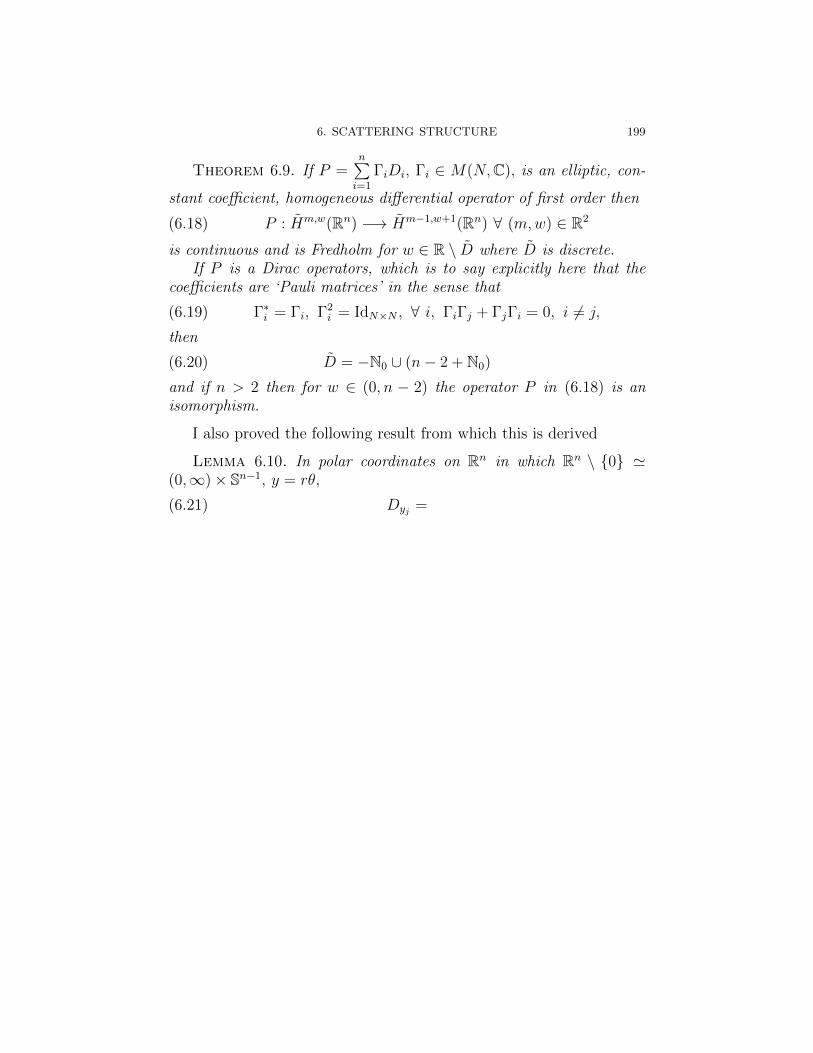
6. SCATTERING STRUCTURE 199
Theorem 6.9. If P =n∑i=1
ΓiDi, Γi ∈ M(N,C), is an elliptic, con-
stant coefficient, homogeneous differential operator of first order then
(6.18) P : Hm,w(Rn) −→ Hm−1,w+1(Rn) ∀ (m,w) ∈ R2
is continuous and is Fredholm for w ∈ R \ D where D is discrete.If P is a Dirac operators, which is to say explicitly here that the
coefficients are ‘Pauli matrices’ in the sense that
(6.19) Γ∗i = Γi, Γ2i = IdN×N , ∀ i, ΓiΓj + ΓjΓi = 0, i 6= j,
then
(6.20) D = −N0 ∪ (n− 2 + N0)
and if n > 2 then for w ∈ (0, n − 2) the operator P in (6.18) is anisomorphism.
I also proved the following result from which this is derived
Lemma 6.10. In polar coordinates on Rn in which Rn \ 0 '(0,∞)× Sn−1, y = rθ,
(6.21) Dyj =

CHAPTER 9
Electromagnetism
1. Maxwell’s equations
Maxwell’s equations in a vacuum take the standard form
(1.1)
div E = ρ div B = 0
curl E = −∂B
∂tcurl B =
∂E
∂t+ J
where E is the electric and B the magnetic field strength, both are3-vectors depending on position z ∈ R3 and time t ∈ R. The externalquantities are ρ, the charge density which is a scalar, and J, the currentdensity which is a vector.
We will be interested here in stationary solutions for which E andB are independent of time and with J = 0, since this also representsmotion in the standard description. Thus we arrive at
(1.2)div E = ρ div B = 0
curl E = 0 curl B = 0.
The simplest interesting solutions represent charged particles, saywith the charge at the origin, ρ = cδ0(z), and with no magnetic field,B = 0. By identifying E with a 1-form, instead of a vector field on R3,
(1.3) E = (E1, E2, E3) =⇒ e = E1dz1 + E2dz2 + E3dz3
we may identify curl E with the 2-form de,
(1.4) de =(∂E2
∂z1
− ∂E1
∂z2
)dz1∧dz2+
(∂E3
∂z2
− ∂E2
∂z3
)dz2∧dz3+
(∂E1
∂z3
− ∂E3
∂z1
)dz3∧dz1.
Thus (1.2) implies that e is a closed 1-form, satisfying
(1.5)∂E1
∂z1
+∂E2
∂z2
+∂E3
∂z3
= cδ0(z).
By the Poincare Lemma, a closed 1-form on R3 is exact, e = dp,with p determined up to an additive constant. If e is smooth (which it
201
202 9. ELECTROMAGNETISM
cannot be, because of (1.5)), then(1.6)
p(z)− p(z′) =
∫ 1
0
γ∗e along γ : [0, 1] −→ R3, γ(0) = z′, γ(1) = z.
It is reasonable to look for a particular p and 1-form e which satisfy(1.5) and are smooth outside the origin. Then (1.6) gives a potentialwhich is well defined, up to an additive constant, outside 0, once z′ isfixed, since de = 0 implies that the integral of γ∗e along a closed curvevanishes. This depends on the fact that R3\0 is simply connected.
So, modulo confirmation of these simple statements, it suffices tolook for p ∈ C∞(R3\0) satisfying e = dp and (1.5), so
(1.7) ∆p = −(∂2p
∂z21
+∂2p
∂z22
+∂2p
∂z23
)= −cδ0(z).
Then E is recovered from e = dp.The operator ‘div’ can also be understood in terms of de Rham d
together with the Hodge star ∗. If we take R3 to have the standard ori-entation and Euclidean metric dz2
1 +dz22 +dz2
3 , the Hodge star operatoris given on 1-forms by
(1.8) ∗dz1 = dz2 ∧ dz3, ∗dz2 = dz3 ∧ dz1, ∗dz3 = dz1 ∧ dz2.
Thus ∗e is a 2-form,
(1.9) ∗ e = E1 dz2 ∧ dz3 + E2 dz3 ∧ dz1 + E3 dz1 ∧ dz2
=⇒ d∗e =
(∂E1
∂z1
+∂E2
∂z2
+∂E3
∂z3
)dz1∧dz2∧dz3 = (div E) dz1∧dz2∧dz3.
The stationary Maxwell’s equations on e become
(1.10) d ∗ e = ρ dz1 ∧ dz2 ∧ dz3, de = 0.
There is essential symmetry in (1.1) except for the appearance of the“source” terms, ρ and J. To reduce (1.1) to two equations, analogousto (1.10) but in 4-dimensional (Minkowski) space requires B to beidentified with a 2-form on R3, rather than a 1-form. Thus, set
(1.11) β = B1 dz2 ∧ dz3 +B2 dz3 ∧ dz1 +B3 dz1 ∧ dz2.
Then
(1.12) dβ = div B dz1 ∧ dz2 ∧ dz3
as follows from (1.9) and the second equation in (1.1) implies β isclosed.
1. MAXWELL’S EQUATIONS 203
Thus e and β are respectively a closed 1-form and a closed 2-formon R3. If we return to the general time-dependent setting then we maydefine a 2-form on R4 by
(1.13) λ = e ∧ dt+ β
where e and β are pulled back by the projection π : R4 → R3. Com-puting directly,
(1.14) dλ = d′e ∧ dt+ d′β +∂β
∂t∧ dt
where d′ is now the differential on R3. Thus
(1.15) dλ = 0⇔ d′e+∂β
∂t= 0, d′β = 0
recovers two of Maxwell’s equations. On the other hand we can definea 4-dimensional analogue of the Hodge star but corresponding to theMinkowski metric, not the Euclidean one. Using the natural analogueof the 3-dimensional Euclidean Hodge by formally inserting an i intothe t-component, gives
(1.16)
∗4dz1 ∧ dz2 = idz3 ∧ dt∗4dz1 ∧ dz3 = idt ∧ dz2
∗4dz1 ∧ dt = −idz2 ∧ dz3
∗4dz2 ∧ dz3 = idz1 ∧ dt∗4dz2 ∧ dt = −idz3 ∧ dz1
∗4dz3 ∧ dt = −idz1 ∧ dz2.
The other two of Maxwell’s equations then become
(1.17) d ∗4 λ = d(−i ∗ e+ i(∗β) ∧ dt) = −i(ρ dz1 ∧ dz2 ∧ dz3 + j ∧ dt)where j is the 1-form associated to J as in (1.3). For our purposes thisis really just to confirm that it is best to think of B as the 2-form βrather than try to make it into a 1-form. There are other good reasonsfor this, related to behaviour under linear coodinate changes.
Returning to the stationary setting, note that (1.7) has a ‘preferred’solution
(1.18) p =1
4π|z|.
This is in fact the only solution which vanishes at infinity.
Proposition 1.1. The only tempered solutions of (1.7) are of theform
(1.19) p =1
4π|z|+ q, ∆q = 0, q a polynomial.
204 9. ELECTROMAGNETISM
Proof. The only solutions are of the form (1.19) where q ∈ S ′(R3)is harmonic. Thus q ∈ S ′(R3) satisfies |ξ|2q = 0, which implies that qis a polynomial.
2. Hodge Theory
The Hodge ∗ operator discussed briefly above in the case of R3 (andMinkowski 4-space) makes sense in any oriented real vector space, V,with a Euclidean inner product—that is, on a finite dimensional realHilbert space. Namely, if e1, . . . , en is an oriented orthonormal basisthen
(2.1) ∗(ei1 ∧ · · · ∧ eik) = sgn(i∗)eik+1∧ · · · ein
extends by linearity to
(2.2) ∗ :∧k V −→
∧n−k V .
Proposition 2.1. The linear map (2.2) is independent of the ori-ented orthonormal basis used to define it and so depends only on thechoice of inner product and orientation of V. Moreover,
(2.3) ∗2 = (−1)k(n−k), on∧k V .
Proof. Note that sgn(i∗), the sign of the permutation defined byi1, . . . , in is fixed by
(2.4) ei1 ∧ · · · ∧ ein = sgn(i∗)e1 ∧ · · · ∧ en.
Thus, on the basis ei1 ∧ . . . ∧ ein of∧k V given by strictly increasing
sequences i1 < i2 < · · · < ik in 1, . . . , n,(2.5) e∗ ∧ ∗e∗ = sgn(i∗)
2e1 ∧ · · · ∧ en = e1 ∧ · · · ∧ en.
The standard inner product on∧k V is chosen so that this basis is
orthonormal. Then (2.5) can be rewritten
(2.6) eI ∧ ∗eJ = 〈eI , eJ〉e1 ∧ · · · ∧ en.This in turn fixes ∗ uniquely since the pairing given by
(2.7)∧k V ×
∧k−1 V 3 (u, v) 7→ (u ∧ v)/e1∧···∧en
is non-degenerate, as can be checked on these bases.Thus it follows from (2.6) that ∗ depends only on the choice of inner
product and orientation as claimed, provided it is shown that the innerproduct on
∧k V only depends on that of V. This is a standard factfollowing from the embedding
(2.8)∧k V → V ⊗k
2. HODGE THEORY 205
as the totally antisymmetric part, the fact that V ⊗k has a natural innerproduct and the fact that this induces one on
∧k V after normalization(depending on the convention used in (2.8). These details are omitted.
Since ∗ is uniquely determined in this way, it necessarily dependssmoothly on the data, in particular the inner product. On an ori-ented Riemannian manifold the induced inner product on T ∗pM variessmoothly with p (by assumption) so
(2.9) ∗ :∧kpM −→
∧n−kp M,
∧kpM =
∧kp(T
∗pM)
varies smoothly and so defines a smooth bundle map
(2.10) ∗ ∈ C∞(M ;∧kM,
∧n−kM).
An oriented Riemannian manifold carries a natural volume formν ∈ C∞(M,
∧nM), and this allows (2.6) to be written in integral form:
(2.11)
∫M
〈α, β〉 ν =
∫M
α ∧ ∗β ∀α, β ∈ C∞(M,∧kM).
Lemma 2.2. On an oriented, (compact) Riemannian manifold theadjoint of d with respect to the Riemannian inner product and volumeform is
(2.12) d∗ = δ = (−1)k+n(n−k+1) ∗ d ∗ on∧kM.
Proof. By definition,
(2.13) d : C∞(M,∧kM) −→ C∞(M,
∧k+1M)
=⇒ δ : C∞(M,∧k+1 M) −→ C∞(M,
∧kM),∫M
〈dα, α′〉 ν =
∫M
〈α, δα′〉 ν ∀α ∈ C∞(M,∧kM), α′ ∈ C∞(M,
∧k+1M).
Applying (2.11) and using Stokes’ theorem, (and compactness of eitherM or the support of at least one of α, α′),∫
M
〈δα, α′〉 ν =
∫M
dα ∧ ∗α′
=
∫M
d(α∧∗α′)+(−1)k+1
∫M
α∧d∗α′ = 0+(−1)k+1
∫M
〈α, ∗−1d∗α′〉 ν.
Taking into account (2.3) to compute ∗−1 on n− k forms shows that
(2.14) δα′ = (−1)k+1+n(n−k) ∗ d ∗ on (k + 1)-forms
which is just (2.12) on k-forms.
206 9. ELECTROMAGNETISM
Notice that changing the orientation simply changes the sign of ∗on all forms. Thus (2.12) does not depend on the orientation and as alocal formula is valid even if M is not orientable — since the existenceof δ = d∗ does not require M to be orientable.
Theorem 2.3 (Hodge/Weyl). On any compact Riemannian man-ifold there is a canonical isomorphism
(2.15) HkdR(M) ∼= Hk
Ho(M) =u ∈ L2(M ;
∧kM); (d+ δ)u = 0
where the left-hand side is either the C∞ or the distributional de Rhamcohomology
(2.16)u ∈ C∞(M ;
∧kM); du = 0/
d C∞(M ;∧kM)
∼=u ∈ C−∞(M ;
∧kM); du = 0/
d C−∞(M ;∧kM).
Proof. The critical point of course is that
(2.17) d+ δ ∈ Diff1(M ;∧∗M) is elliptic.
We know that the symbol of d at a point ζ ∈ T ∗pM is the map
(2.18)∧kM 3 α 7→ iζ ∧ α.
We are only interested in ζ 6= 0 and by homogeneity it is enough toconsider |ζ| = 1. Let e1 = ζ, e2, . . . , en be an orthonormal basis ofT ∗pM , then from (2.12) with a fixed sign throughout:
(2.19) σ(δ, ζ)α = ± ∗ (iζ ∧ ·) ∗ α.
Take α = eI , ∗α = ±eI′ where I ∪ I ′ = 1, . . . , n. Thus
(2.20) σ(δ, ζ)α = 0 1 6∈ I±iαI\1 1 ∈ I .
In particular, σ(d+ δ) is an isomorphism since it satisfies
(2.21) σ(d+ δ)2 = |ζ|2
as follows from (2.18) and (2.20) or directly from the fact that
(2.22) (d+ δ)2 = d2 + dδ + δd+ δ2 = dδ + δd
again using (2.18) and (2.20).Once we know that d+ δ is elliptic we conclude from the discussion
of Fredholm properties above that the distributional null space
(2.23)u ∈ C−∞(M,
∧∗M); (d+ δ)u = 0⊂ C∞(M,
∧∗M)
2. HODGE THEORY 207
is finite dimensional. From this it follows that
(2.24)Hk
Ho =u ∈ C−∞(M,∧kM); (d+ δ)u = 0
=u ∈ C∞(M,∧kM); du = δu = 0
and that the null space in (2.23) is simply the direct sum of these spacesover k. Indeed, from (2.23) the integration by parts in
0 =
∫〈du, (d+ δ)u〉 ν = ‖du‖2
L2 +
∫〈u, δ2u〉 ν = ‖du‖2
L2
is justified.Thus we can consider d+ δ as a Fredholm operator in three forms
(2.25)
d+ δ :C−∞(M,∧∗M) −→ C−∞(M,
∧∗M),
d+ δ :H1(M,∧∗M) −→ H1(M,
∧∗M),
d+ δ :C∞(M,∧∗M) −→ C∞(M,
∧∗M)
and obtain the three direct sum decompositions
(2.26)
C−∞(M,∧∗M) = H∗Ho ⊕ (d+ δ)C−∞(M,
∧∗M),
L2(M,∧∗M) = H∗Ho ⊕ (d+ δ)L2(M,
∧∗M),
C∞(M,∧∗M) = H∗Ho ⊕ (d+ δ)C∞(M,
∧∗M).
The same complement occurs in all three cases in view of (2.24).From (2.24) directly, all the “harmonic” forms in Hk
Ho(M) are closedand so there is a natural map
(2.27) HkHo(M) −→ Hk
dR(M) −→ HkdR,C−∞(M)
where the two de Rham spaces are those in (2.16), not yet shown to beequal.
We proceed to show that the maps in (2.27) are isomorphisms. Firstto show injectivity, suppose u ∈ Hk
Ho(M) is mapped to zero in eitherspace. This means u = dv where v is either C∞ or distributional, soit suffices to suppose v ∈ C−∞(M,
∧k−1M). Since u is smooth theintegration by parts in the distributional pairing
‖u‖2L2 =
∫M
〈u, dv〉 ν =
∫M
〈δu, v〉 ν = 0
is justified, so u = 0 and the maps are injective.To see surjectivity, use the Hodge decomposition (2.26). If u′ ∈
C−∞(M,∧kM) or C∞(M,
∧kM), we find
(2.28) u′ = u0 + (d+ δ)v
where correspondingly, v ∈ C−∞(M,∧∗M) or C∞(M,
∧∗M) and u0 ∈Hk
Ho(M). If u′ is closed, du′ = 0, then dδv = 0 follows from applying
208 9. ELECTROMAGNETISM
d to (2.28) and hence (d + δ)δv = 0, since δ2 = 0. Thus δv ∈ H∗Ho(M)and in particular, δv ∈ C∞(M,
∧∗M). Then the integration by partsin
‖δv‖2L2 =
∫〈δv, δv〉 ν =
∫〈v, (d+ δ)δv〉 ν = 0
is justified, so δv = 0. Then (2.28) shows that any closed form, smoothor distributional, is cohomologous in the same sense to u0 ∈ Hk
Ho(M).Thus the natural maps (2.27) are isomorphisms and the Theorem isproved.
Thus, on a compact Riemannian manifold (whether orientable ornot), each de Rham class has a unique harmonic representative.
3. Coulomb potential
4. Dirac strings
Addenda to Chapter 9
CHAPTER 10
Monopoles
1. Gauge theory
2. Bogomolny equations
(1) Compact operators, spectral theorem(2) Families of Fredholm operators(*)(3) Non-compact self-adjoint operators, spectral theorem(4) Spectral theory of the Laplacian on a compact manifold(5) Pseudodifferential operators(*)(6) Invertibility of the Laplacian on Euclidean space(7) Lie groups(), bundles and gauge invariance(8) Bogomolny equations on R3
(9) Gauge fixing(10) Charge and monopoles(11) Monopole moduli spaces
* I will drop these if it looks as though time will become an issue., I will provide a brief and elementary discussion of manifolds and Liegroups if that is found to be necessary.
3. Problems
Problem 1. Prove that u+, defined by (15.10) is linear.
Problem 2. Prove Lemma 15.7.Hint(s). All functions here are supposed to be continuous, I just
don’t bother to keep on saying it.
(1) Recall, or check, that the local compactness of a metric spaceX means that for each point x ∈ X there is an ε > 0 such thatthe ball y ∈ X; d(x, y) ≤ δ is compact for δ ≤ ε.
(2) First do the case n = 1, so K b U is a compact set in an opensubset.(a) Given δ > 0, use the local compactness of X, to cover K
with a finite number of compact closed balls of radius atmost δ.
209
210 10. MONOPOLES
(b) Deduce that if ε > 0 is small enough then the set x ∈X; d(x,K) ≤ ε, where
d(x,K) = infy∈K
d(x, y),
is compact.(c) Show that d(x,K), for K compact, is continuous.(d) Given ε > 0 show that there is a continuous function
gε : R −→ [0, 1] such that gε(t) = 1 for t ≤ ε/2 andgε(t) = 0 for t > 3ε/4.
(e) Show that f = gεd(·, K) satisfies the conditions for n = 1if ε > 0 is small enough.
(3) Prove the general case by induction over n.(a) In the general case, set K ′ = K ∩ U 1 and show that the
inductive hypothesis applies toK ′ and the Uj for j > 1; letf ′j, j = 2, . . . , n be the functions supplied by the inductiveassumption and put f ′ =
∑j≥2 f
′j.
(b) Show that K1 = K ∩ f ′ ≤ 12 is a compact subset of U1.
(c) Using the case n = 1 construct a function F for K1 andU1.
(d) Use the case n = 1 again to find G such that G = 1 on Kand supp(G) b f ′ + F > 1
2.
(e) Make sense of the functions
f1 = FG
f ′ + F, fj = f ′j
G
f ′ + F, j ≥ 2
and show that they satisfies the inductive assumptions.
Problem 3. Show that σ-algebras are closed under countable in-tersections.
Problem 4. (Easy) Show that if µ is a complete measure andE ⊂ F where F is measurable and has measure 0 then µ(E) = 0.
Problem 5. Show that compact subsets are measurable for anyBorel measure. (This just means that compact sets are Borel sets ifyou follow through the tortuous terminology.)
Problem 6. Show that the smallest σ-algebra containing the sets
(a,∞] ⊂ [−∞,∞]
for all a ∈ R, generates what is called above the ‘Borel’ σ-algebra on[−∞,∞].
Problem 7. Write down a careful proof of Proposition 1.1.
3. PROBLEMS 211
Problem 8. Write down a careful proof of Proposition 1.2.
Problem 9. Let X be the metric space
X = 0 ∪ 1/n;n ∈ N = 1, 2, . . . ⊂ Rwith the induced metric (i.e. the same distance as on R). Recall whyX is compact. Show that the space C0(X) and its dual are infinitedimensional. Try to describe the dual space in terms of sequences; atleast guess the answer.
Problem 10. For the space Y = N = 1, 2, . . . ⊂ R, describeC0(Y ) and guess a description of its dual in terms of sequences.
Problem 11. Let (X,M, µ) be any measure space (so µ is a mea-sure on the σ-algebraM of subsets of X). Show that the set of equiv-alence classes of µ-integrable functions on X, with the equivalence re-lation given by (4.8), is a normed linear space with the usual linearstructure and the norm given by
‖f‖ =
∫X
|f |dµ.
Problem 12. Let (X,M) be a set with a σ-algebra. Let µ :M→R be a finite measure in the sense that µ(φ) = 0 and for any Ei∞i=1 ⊂M with Ei ∩ Ej = φ for i 6= j,
(3.1) µ
(∞⋃i=1
Ei
)=∞∑i=1
µ(Ei)
with the series on the right always absolutely convergenct (i.e., this ispart of the requirement on µ). Define
(3.2) |µ| (E) = sup∞∑i=1
|µ(Ei)|
for E ∈ M, with the supremum over all measurable decompositionsE =
⋃∞i=1Ei with the Ei disjoint. Show that |µ| is a finite, positive
measure.Hint 1. You must show that |µ| (E) =
∑∞i=1 |µ| (Ai) if
⋃iAi = E,
Ai ∈ M being disjoint. Observe that if Aj =⋃lAjl is a measurable
decomposition of Aj then together the Ajl give a decomposition of E.Similarly, if E =
⋃j Ej is any such decomposition of E then Ajl =
Aj ∩ El gives such a decomposition of Aj.Hint 2. See [6] p. 117!
Problem 13. (Hahn Decomposition)With assumptions as in Problem 12:
212 10. MONOPOLES
(1) Show that µ+ = 12(|µ| + µ) and µ− = 1
2(|µ| − µ) are positive
measures, µ = µ+ − µ−. Conclude that the definition of ameasure based on (4.16) is the same as that in Problem 12.
(2) Show that µ± so constructed are orthogonal in the sense thatthere is a set E ∈M such that µ−(E) = 0, µ+(X \ E) = 0.
Hint. Use the definition of |µ| to show that for any F ∈Mand any ε > 0 there is a subset F ′ ∈ M, F ′ ⊂ F such thatµ+(F ′) ≥ µ+(F ) − ε and µ−(F ′) ≤ ε. Given δ > 0 applythis result repeatedly (say with ε = 2−nδ) to find a decreasingsequence of sets F1 = X, Fn ∈ M, Fn+1 ⊂ Fn such thatµ+(Fn) ≥ µ+(Fn−1)−2−nδ and µ−(Fn) ≤ 2−nδ. Conclude thatG =
⋂n Fn has µ+(G) ≥ µ+(X) − δ and µ−(G) = 0. Now let
Gm be chosen this way with δ = 1/m. Show that E =⋃mGm
is as required.
Problem 14. Now suppose that µ is a finite, positive Radon mea-sure on a locally compact metric space X (meaning a finite positiveBorel measure outer regular on Borel sets and inner regular on opensets). Show that µ is inner regular on all Borel sets and hence, givenε > 0 and E ∈ B(X) there exist sets K ⊂ E ⊂ U with K compact andU open such that µ(K) ≥ µ(E)− ε, µ(E) ≥ µ(U)− ε.
Hint. First take U open, then use its inner regularity to find Kwith K ′ b U and µ(K ′) ≥ µ(U) − ε/2. How big is µ(E\K ′)? FindV ⊃ K ′\E with V open and look at K = K ′\V .
Problem 15. Using Problem 14 show that if µ is a finite Borelmeasure on a locally compact metric space X then the following threeconditions are equivalent
(1) µ = µ1 − µ2 with µ1 and µ2 both positive finite Radon mea-sures.
(2) |µ| is a finite positive Radon measure.(3) µ+ and µ− are finite positive Radon measures.
Problem 16. Let ‖ ‖ be a norm on a vector space V . Show that‖u‖ = (u, u)1/2 for an inner product satisfying (1.1) - (1.4) if and onlyif the parallelogram law holds for every pair u, v ∈ V .
Hint (From Dimitri Kountourogiannis)If ‖ · ‖ comes from an inner product, then it must satisfy the polar-
isation identity:
(x, y) = 1/4(‖x+ y‖2 − ‖x− y‖2 − i‖x+ iy‖2 − i‖x− iy‖2)
i.e, the inner product is recoverable from the norm, so use the RHS(right hand side) to define an inner product on the vector space. You
3. PROBLEMS 213
will need the paralellogram law to verify the additivity of the RHS.Note the polarization identity is a bit more transparent for real vectorspaces. There we have
(x, y) = 1/2(‖x+ y‖2 − ‖x− y‖2)
both are easy to prove using ‖a‖2 = (a, a).
Problem 17. Show (Rudin does it) that if u : Rn → C has con-tinuous partial derivatives then it is differentiable at each point in thesense of (6.19).
Problem 18. Consider the function f(x) = 〈x〉−1 = (1 + |x|2)−1/2.Show that
∂f
∂xj= lj(x) · 〈x〉−3
with lj(x) a linear function. Conclude by induction that 〈x〉−1 ∈Ck0 (Rn) for all k.
Problem 19. Show that exp(− |x|2) ∈ S(Rn).
Problem 20. Prove (2.8), probably by induction over k.
Problem 21. Prove Lemma 2.4.
Hint. Show that a set U 3 0 in S(Rn) is a neighbourhood of 0 ifand only if for some k and ε > 0 it contains a set of the formϕ ∈ S(Rn) ;
∑|α|≤k,|β|≤k
sup∣∣xαDβϕ
∣∣ < ε
.
Problem 22. Prove (3.7), by estimating the integrals.
Problem 23. Prove (3.9) where
ψj(z;x′) =
∫ ′0
∂ψ
∂zj(z + tx′) dt .
Problem 24. Prove (3.20). You will probably have to go back tofirst principles to do this. Show that it is enough to assume u ≥ 0 hascompact support. Then show it is enough to assume that u is a simple,and integrable, function. Finally look at the definition of Lebesguemeasure and show that if E ⊂ Rn is Borel and has finite Lebesguemeasure then
lim|t|→∞
µ(E\(E + t)) = 0
where µ = Lebesgue measure and
E + t = p ∈ Rn ; p′ + t , p′ ∈ E .
214 10. MONOPOLES
Problem 25. Prove Leibniz’ formula
Dαx(ϕψ) =
∑β≤α
(α
β
)Dα
xϕ · dα−βx ψ
for any C∞ functions and ϕ and ψ. Here α and β are multiindices,β ≤ α means βj ≤ αj for each j? and(
α
β
)=∏j
(αjβj
).
I suggest induction!
Problem 26. Prove the generalization of Proposition 3.10 thatu ∈ S ′(Rn), supp(w) ⊂ 0 implies there are constants cα , |α| ≤ m,for some m, such that
u =∑|α|≤m
cαDαδ .
Hint This is not so easy! I would be happy if you can show thatu ∈ M(Rn), suppu ⊂ 0 implies u = cδ. To see this, you can showthat
ϕ ∈ S(Rn), ϕ(0) = 0
⇒ ∃ϕj ∈ S(Rn) , ϕj(x) = 0 in |x| ≤ εj > 0(↓ 0) ,
sup |ϕj − ϕ| → 0 as j →∞ .
To prove the general case you need something similar — that given m,if ϕ ∈ S(Rn) and Dα
xϕ(0) = 0 for |α| ≤ m then ∃ϕj ∈ S(Rn), ϕj = 0in |x| ≤ εj , εj ↓ 0 such that ϕj → ϕ in the Cm norm.
Problem 27. If m ∈ N, m′ > 0 show that u ∈ Hm(Rn) andDαu ∈ Hm′(Rn) for all |α| ≤ m implies u ∈ Hm+m′(Rn). Is theconverse true?
Problem 28. Show that every element u ∈ L2(Rn) can be writtenas a sum
u = u0 +n∑j=1
Djuj , uj ∈ H1(Rn) , j = 0, . . . , n .
Problem 29. Consider for n = 1, the locally integrable function(the Heaviside function),
H(x) =
0 x ≤ 01 x > 1 .
Show that DxH(x) = cδ; what is the constant c?
3. PROBLEMS 215
Problem 30. For what range of orders m is it true that δ ∈Hm(Rn) , δ(ϕ) = ϕ(0)?
Problem 31. Try to write the Dirac measure explicitly (as possi-ble) in the form (5.8). How many derivatives do you think are neces-sary?
Problem 32. Go through the computation of ∂E again, but cut-ting out a disk x2 + y2 ≤ ε2 instead.
Problem 33. Consider the Laplacian, (6.4), for n = 3. Show thatE = c(x2 + y2)−1/2 is a fundamental solution for some value of c.
Problem 34. Recall that a topology on a set X is a collection F ofsubsets (called the open sets) with the properties, φ ∈ F , X ∈ F andF is closed under finite intersections and arbitrary unions. Show thatthe following definition of an open set U ⊂ S ′(Rn) defines a topology:
∀ u ∈ U and all ϕ ∈ S(Rn) ∃ε > 0 st.
|(u′ − u)(ϕ)| < ε⇒ u′ ∈ U .This is called the weak topology (because there are very few opensets). Show that uj → u weakly in S ′(Rn) means that for every openset U 3 u ∃N st. uj ∈ U ∀ j ≥ N .
Problem 35. Prove (6.18) where u ∈ S ′(Rn) and ϕ, ψ ∈ S(Rn).
Problem 36. Show that for fixed v ∈ S ′(Rn) with compact support
S(Rn) 3 ϕ 7→ v ∗ ϕ ∈ S(Rn)
is a continuous linear map.
Problem 37. Prove the ?? to properties in Theorem 6.6 for u ∗ vwhere u ∈ S ′(Rn) and v ∈ S ′(Rn) with at least one of them havingcompact support.
Problem 38. Use Theorem 6.9 to show that if P (D) is hypoellipticthen every parametrix F ∈ S(Rn) has sing supp(F ) = 0.
Problem 39. Show that if P (D) is an ellipitic differential operatorof order m, u ∈ L2(Rn) and P (D)u ∈ L2(Rn) then u ∈ Hm(Rn).
Problem 40 (Taylor’s theorem). . Let u : Rn −→ R be a real-valued function which is k times continuously differentiable. Prove thatthere is a polynomial p and a continuous function v such that
u(x) = p(x) + v(x) where lim|x|↓0
|v(x)||x|k
= 0.
216 10. MONOPOLES
Problem 41. Let C(Bn) be the space of continuous functions onthe (closed) unit ball, Bn = x ∈ Rn; |x| ≤ 1. Let C0(Bn) ⊂ C(Bn) bethe subspace of functions which vanish at each point of the boundaryand let C(Sn−1) be the space of continuous functions on the unit sphere.Show that inclusion and restriction to the boundary gives a short exactsequence
C0(Bn) → C(Bn) −→ C(Sn−1)
(meaning the first map is injective, the second is surjective and theimage of the first is the null space of the second.)
Problem 42 (Measures). A measure on the ball is a continuouslinear functional µ : C(Bn) −→ R where continuity is with respect tothe supremum norm, i.e. there must be a constant C such that
|µ(f)| ≤ C supx∈Rn|f(x)| ∀ f ∈ C(Bn).
Let M(Bn) be the linear space of such measures. The space M(Sn−1)of measures on the sphere is defined similarly. Describe an injectivemap
M(Sn−1) −→M(Bn).
Can you define another space so that this can be extended to a shortexact sequence?
Problem 43. Show that the Riemann integral defines a measure
(3.3) C(Bn) 3 f 7−→∫Bnf(x)dx.
Problem 44. If g ∈ C(Bn) and µ ∈M(Bn) show that gµ ∈M(Bn)where (gµ)(f) = µ(fg) for all f ∈ C(Bn). Describe all the measureswith the property that
xjµ = 0 in M(Bn) for j = 1, . . . , n.
Problem 45 (Hormander, Theorem 3.1.4). Let I ⊂ R be an open,non-empty interval.
i) Show (you may use results from class) that there exists ψ ∈C∞c (I) with
∫R ψ(x)ds = 1.
ii) Show that any φ ∈ C∞c (I) may be written in the form
φ = φ+ cψ, c ∈ C, φ ∈ C∞c (I) with
∫Rφ = 0.
iii) Show that if φ ∈ C∞c (I) and∫R φ = 0 then there exists µ ∈
C∞c (I) such that dµdx
= φ in I.
3. PROBLEMS 217
iv) Suppose u ∈ C−∞(I) satisfies dudx
= 0, i.e.
u(−dφdx
) = 0 ∀ φ ∈ C∞c (I),
show that u = c for some constant c.v) Suppose that u ∈ C−∞(I) satisfies du
dx= c, for some constant
c, show that u = cx+ d for some d ∈ C.
Problem 46. [Hormander Theorem 3.1.16]
i) Use Taylor’s formula to show that there is a fixed ψ ∈ C∞c (Rn)such that any φ ∈ C∞c (Rn) can be written in the form
φ = cψ +n∑j=1
xjψj
where c ∈ C and the ψj ∈ C∞c (Rn) depend on φ.ii) Recall that δ0 is the distribution defined by
δ0(φ) = φ(0) ∀ φ ∈ C∞c (Rn);
explain why δ0 ∈ C−∞(Rn).iii) Show that if u ∈ C−∞(Rn) and u(xjφ) = 0 for all φ ∈ C∞c (Rn)
and j = 1, . . . , n then u = cδ0 for some c ∈ C.iv) Define the ‘Heaviside function’
H(φ) =
∫ ∞0
φ(x)dx ∀ φ ∈ C∞c (R);
show that H ∈ C−∞(R).v) Compute d
dxH ∈ C−∞(R).
Problem 47. Using Problems 45 and 46, find all u ∈ C−∞(R)satisfying the differential equation
xdu
dx= 0 in R.
These three problems are all about homogeneous distributions onthe line, extending various things using the fact that
xz+ =
exp(z log x) x > 0
0 x ≤ 0
is a continuous function on R if Re z > 0 and is differentiable if Re z > 1and then satisfies
d
dxxz+ = zxz−1
+ .
218 10. MONOPOLES
We used this to define
(3.4) xz+ =1
z + k
1
z + k − 1· · · 1
z + 1
dk
dxkxz+k+ if z ∈ C \ −N.
Problem 48. [Hadamard regularization]
i) Show that (3.4) just means that for each φ ∈ C∞c (R)
xz+(φ) =(−1)k
(z + k) · · · (z + 1)
∫ ∞0
dkφ
dxk(x)xz+kdx, Re z > −k, z /∈ −N.
ii) Use integration by parts to show that(3.5)
xz+(φ) = limε↓0
[∫ ∞ε
φ(x)xzdx−k∑j=1
Cj(φ)εz+j
], Re z > −k, z /∈ −N
for certain constants Cj(φ) which you should give explicitly.[This is called Hadamard regularization after Jacques Hadamard,feel free to look at his classic book [3].]
iii) Assuming that −k + 1 ≥ Re z > −k, z 6= −k + 1, show thatthere can only be one set of the constants with j < k (for eachchoice of φ ∈ C∞c (R)) such that the limit in (3.5) exists.
iiv) Use ii), and maybe iii), to show that
d
dxxz+ = zxz−1
+ in C−∞(R) ∀ z /∈ −N0 = 0, 1, . . . .
v) Similarly show that xxz+ = xz+1+ for all z /∈ −N.
vi) Show that xz+ = 0 in x < 0 for all z /∈ −N. (Duh.)
Problem 49. [Null space of x ddx− z]
i) Show that if u ∈ C−∞(R) then u(φ) = u(φ), where φ(x) =φ(−x) ∀ φ ∈ C∞c (R), defines an element of C−∞(R). What is
u if u ∈ C0(R)? Compute δ0.
ii) Show that ddxu = − d
dxu.
iii) Define xz− = xz+ for z /∈ −N and show that ddxxz− = −zxz−1
−and xxz− = −xz+1
− .iv) Suppose that u ∈ C−∞(R) satisfies the distributional equation
(x ddx− z)u = 0 (meaning of course, xdu
dx= zu where z is a
constant). Show that
u∣∣x>0
= c+xz−∣∣x>0
and u∣∣x<0
= c−xz−∣∣x<0
3. PROBLEMS 219
for some constants c±. Deduce that v = u − c+xz+ − c−x
z−
satisfies
(3.6) (xd
dx− z)v = 0 and supp(v) ⊂ 0.
v) Show that for each k ∈ N, (x ddx
+ k + 1) dk
dxkδ0 = 0.
vi) Using the fact that any v ∈ C−∞(R) with supp(v) ⊂ 0 is
a finite sum of constant multiples of the dk
dxkδ0, show that, for
z /∈ −N, the only solution of (3.6) is v = 0.vii) Conclude that for z /∈ −N
(3.7)
u ∈ C−∞(R); (x
d
dx− z)u = 0
is a two-dimensional vector space.
Problem 50. [Negative integral order] To do the same thing fornegative integral order we need to work a little differently. Fix k ∈ N.
i) We define weak convergence of distributions by saying un → uin C∞c (X), where un, u ∈ C−∞(X), X ⊂ Rn being open, ifun(φ)→ u(φ) for each φ ∈ C∞c (X). Show that un → u impliesthat ∂un
∂xj→ ∂u
∂xjfor each j = 1, . . . , n and fun → fu if f ∈
C∞(X).ii) Show that (z + k)xz+ is weakly continuous as z → −k in the
sense that for any sequence zn → −k, zn /∈ −N, (zn +k)xzn+ →vk where
vk =1
−1· · · 1
−k + 1
dk+1
dxk+1x+, x+ = x1
+.
iii) Compute vk, including the constant factor.iv) Do the same thing for (z + k)xz− as z → −k.v) Show that there is a linear combination (k + z)(xz+ + c(k)xz−)
such that as z → −k the limit is zero.vi) If you get this far, show that in fact xz+ + c(k)xz− also has a
weak limit, uk, as z → −k. [This may be the hardest part.]vii) Show that this limit distribution satisfies (x d
dx+ k)uk = 0.
viii) Conclude that (3.7) does in fact hold for z ∈ −N as well.[There are still some things to prove to get this.]
Problem 51. Show that for any set G ⊂ Rn
v∗(G) = inf∞∑i=1
v(Ai)
where the infimum is taken over coverings of G by rectangular sets(products of intervals).
220 10. MONOPOLES
Problem 52. Show that a σ-algebra is closed under countable in-tersections.
Problem 53. Show that compact sets are Lebesgue measurableand have finite volume and also show the inner regularity of the Lebesguemeasure on open sets, that is if E is open then
(3.8) v(E) = supv(K);K ⊂ E, K compact.
Problem 54. Show that a set B ⊂ Rn is Lebesgue measurable ifand only if
v∗(E) = v∗(E ∩B) + v∗(E ∩B) ∀ open E ⊂ Rn.
[The definition is this for all E ⊂ Rn.]
Problem 55. Show that a real-valued continuous function f :U −→ R on an open set, is Lebesgue measurable, in the sense thatf−1(I) ⊂ U ⊂ Rn is measurable for each interval I.
Problem 56. Hilbert space and the Riesz representation theorem.If you need help with this, it can be found in lots of places – for instance[7] has a nice treatment.
i) A pre-Hilbert space is a vector space V (over C) with a ‘posi-tive definite sesquilinear inner product’ i.e. a function
V × V 3 (v, w) 7→ 〈v, w〉 ∈ C
satisfying• 〈w, v〉 = 〈v, w〉• 〈a1v1 + a2v2, w〉 = a1〈v1, w〉+ a2〈v2, w〉• 〈v, v〉 ≥ 0• 〈v, v〉 = 0⇒ v = 0.Prove Schwarz’ inequality, that
|〈u, v〉| ≤ 〈u〉12 〈v〉
12 ∀ u, v ∈ V.
Hint: Reduce to the case 〈v, v〉 = 1 and then expand
〈u− 〈u, v〉v, u− 〈u, v〉v〉 ≥ 0.
ii) Show that ‖v‖ = 〈v, v〉1/2 is a norm and that it satisfies theparallelogram law:
(3.9) ‖v1 + v2‖2 + ‖v1 − v2‖2 = 2‖v1‖2 + 2‖v2‖2 ∀ v1, v2 ∈ V.iii) Conversely, suppose that V is a linear space over C with a
norm which satisfies (3.9). Show that
4〈v, w〉 = ‖v + w‖2 − ‖v − w‖2 + i‖v + iw‖2 − i‖v − iw‖2
3. PROBLEMS 221
defines a pre-Hilbert inner product which gives the originalnorm.
iv) Let V be a Hilbert space, so as in (i) but complete as well.Let C ⊂ V be a closed non-empty convex subset, meaningv, w ∈ C ⇒ (v + w)/2 ∈ C. Show that there exists a uniquev ∈ C minimizing the norm, i.e. such that
‖v‖ = infw∈C‖w‖.
Hint: Use the parallelogram law to show that a norm min-imizing sequence is Cauchy.
v) Let u : H → C be a continuous linear functional on a Hilbertspace, so |u(ϕ)| ≤ C‖ϕ‖ ∀ ϕ ∈ H. Show that N = ϕ ∈H;u(ϕ) = 0 is closed and that if v0 ∈ H has u(v0) 6= 0 theneach v ∈ H can be written uniquely in the form
v = cv0 + w, c ∈ C, w ∈ N.
vi) With u as in v), not the zero functional, show that there existsa unique f ∈ H with u(f) = 1 and 〈w, f〉 = 0 for all w ∈ N .
Hint: Apply iv) to C = g ∈ V ;u(g) = 1.vii) Prove the Riesz Representation theorem, that every continu-
ous linear functional on a Hilbert space is of the form
uf : H 3 ϕ 7→ 〈ϕ, f〉 for a unique f ∈ H.
Problem 57. Density of C∞c (Rn) in Lp(Rn).
i) Recall in a few words why simple integrable functions are densein L1(Rn) with respect to the norm ‖f‖L1 =
∫Rn |f(x)|dx.
ii) Show that simple functions∑N
j=1 cjχ(Uj) where the Uj are
open and bounded are also dense in L1(Rn).iii) Show that if U is open and bounded then F (y) = v(U ∩ Uy),
where Uy = z ∈ Rn; z = y + y′, y′ ∈ U is continuous iny ∈ Rn and that
v(U ∩ U y ) + v(U ∩ Uy)→ 0 as y → 0.
iv) If U is open and bounded and ϕ ∈ C∞c (Rn) show that
f(x) =
∫U
ϕ(x− y)dy ∈ C∞c (Rn).
v) Show that if U is open and bounded then
sup|y|≤δ
∫|χU(x)− χU(x− y)|dx→ 0 as δ ↓ 0.
222 10. MONOPOLES
vi) If U is open and bounded and ϕ ∈ C∞c (Rn), ϕ ≥ 0,∫ϕ = 1
then
fδ → χU in L1(Rn) as δ ↓ 0
where
fδ(x) = δ−n∫ϕ(yδ
)χU(x− y)dy.
Hint: Write χU(x) = δ−n∫ϕ(yδ
)χU(x) and use v).
vii) Conclude that C∞c (Rn) is dense in L1(Rn).viii) Show that C∞c (Rn) is dense in Lp(Rn) for any 1 ≤ p <∞.
Problem 58. Schwartz representation theorem. Here we (well you)come to grips with the general structure of a tempered distribution.
i) Recall briefly the proof of the Sobolev embedding theorem andthe corresponding estimate
supx∈Rn|φ(x)| ≤ C‖φ‖Hm ,
n
2< m ∈ R.
ii) For m = n + 1 write down a(n equivalent) norm on the rightin a form that does not involve the Fourier transform.
iii) Show that for any α ∈ N0
|Dα((1 + |x|2)Nφ
)| ≤ Cα,N
∑β≤α
(1 + |x|2)N |Dβφ|.
iv) Deduce the general estimates
sup|α|≤Nx∈Rn
(1 + |x|2)N |Dαφ(x)| ≤ CN‖(1 + |x|2)Nφ‖HN+n+1 .
v) Conclude that for each tempered distribution u ∈ S ′(Rn) thereis an integer N and a constant C such that
|u(φ)| ≤ C‖(1 + |x|2)Nφ‖H2N ∀ φ ∈ S(Rn).
vi) Show that v = (1 + |x|2)−Nu ∈ S ′(Rn) satisfies
|v(φ)| ≤ C‖(1 + |D|2)Nφ‖L2 ∀ φ ∈ S(Rn).
vi) Recall (from class or just show it) that if v is a tempereddistribution then there is a unique w ∈ S ′(Rn) such that (1 +|D|2)Nw = v.
vii) Use the Riesz Representation Theorem to conclude that foreach tempered distribution u there exists N and w ∈ L2(Rn)such that
(3.10) u = (1 + |D|2)N(1 + |x|2)Nw.
3. PROBLEMS 223
viii) Use the Fourier transform on S ′(Rn) (and the fact that it isan isomorphism on L2(Rn)) to show that any tempered distri-bution can be written in the form
u = (1 + |x|2)N(1 + |D|2)Nw for some N and some w ∈ L2(Rn).
ix) Show that any tempered distribution can be written in theform
u = (1+|x|2)N(1+|D|2)N+n+1w for some N and some w ∈ H2(n+1)(Rn).
x) Conclude that any tempered distribution can be written in theform
u = (1 + |x|2)N(1 + |D|2)MU for some N,M
and a bounded continuous function U
Problem 59. Distributions of compact support.
i) Recall the definition of the support of a distribution, definedin terms of its complement
Rn\supp(u) =p ∈ Rn;∃ U ⊂ Rn, open, with p ∈ U such that u
∣∣U
= 0
ii) Show that if u ∈ C−∞(Rn) and φ ∈ C∞c (Rn) satisfy
supp(u) ∩ supp(φ) = ∅then u(φ) = 0.
iii) Consider the space C∞(Rn) of all smooth functions on Rn,without restriction on supports. Show that for each N
‖f‖(N) = sup|α|≤N, |x|≤N
|Dαf(x)|
is a seminorn on C∞(Rn) (meaning it satisfies ‖f‖ ≥ 0, ‖cf‖ =|c|‖f‖ for c ∈ C and the triangle inequality but that ‖f‖ = 0does not necessarily imply that f = 0.)
iv) Show that C∞c (Rn) ⊂ C∞(Rn) is dense in the sense that foreach f ∈ C∞(Rn) there is a sequence fn in C∞c (Rn) such that‖f − fn‖(N) → 0 for each N.
v) Let E ′(Rn) temporarily (or permanantly if you prefer) denotethe dual space of C∞(Rn) (which is also written E(Rn)), thatis, v ∈ E ′(Rn) is a linear map v : C∞(Rn) −→ C which iscontinuous in the sense that for some N
(3.11) |v(f)| ≤ C‖f‖(N) ∀ f ∈ C∞(Rn).
Show that such a v ‘is’ a distribution and that the map E ′(Rn) −→C−∞(Rn) is injective.
224 10. MONOPOLES
vi) Show that if v ∈ E ′(Rn) satisfies (3.11) and f ∈ C∞(Rn) hasf = 0 in |x| < N + ε for some ε > 0 then v(f) = 0.
vii) Conclude that each element of E ′(Rn) has compact supportwhen considered as an element of C−∞(Rn).
viii) Show the converse, that each element of C−∞(Rn) with com-pact support is an element of E ′(Rn) ⊂ C−∞(Rn) and henceconclude that E ′(Rn) ‘is’ the space of distributions of compactsupport.
I will denote the space of distributions of compact support by C−∞c (R).
Problem 60. Hypoellipticity of the heat operator H = iDt +∆ =
iDt +n∑j=1
D2xj
on Rn+1.
(1) Using τ to denote the ‘dual variable’ to t and ξ ∈ Rn to denotethe dual variables to x ∈ Rn observe that H = p(Dt, Dx) wherep = iτ + |ξ|2.
(2) Show that |p(τ, ξ)| > 12
(|τ |+ |ξ|2) .(3) Use an inductive argument to show that, in (τ, ξ) 6= 0 where
it makes sense,
(3.12) DkτD
αξ
1
p(τ, ξ)=
|α|∑j=1
qk,α,j(ξ)
p(τ, ξ)k+j+1
where qk,α,j(ξ) is a polynomial of degree (at most) 2j − |α|.(4) Conclude that if φ ∈ C∞c (Rn+1) is identically equal to 1 in a
neighbourhood of 0 then the function
g(τ, ξ) =1− φ(τ, ξ)
iτ + |ξ|2
is the Fourier transform of a distribution F ∈ S ′(Rn) withsing supp(F ) ⊂ 0. [Remember that sing supp(F ) is the com-plement of the largest open subset of Rn the restriction of Fto which is smooth].
(5) Show that F is a parametrix for the heat operator.(6) Deduce that iDt +∆ is hypoelliptic – that is, if U ⊂ Rn is an
open set and u ∈ C−∞(U) satisfies (iDt + ∆)u ∈ C∞(U) thenu ∈ C∞(U).
(7) Show that iDt −∆ is also hypoelliptic.
Problem 61. Wavefront set computations and more – all prettyeasy, especially if you use results from class.
i) Compute WF(δ) where δ ∈ S ′(Rn) is the Dirac delta functionat the origin.
3. PROBLEMS 225
ii) Compute WF(H(x)) where H(x) ∈ S ′(R) is the Heavisidefunction
H(x) =
1 x > 0
0 x ≤ 0.
Hint: Dx is elliptic in one dimension, hit H with it.iii) Compute WF(E), E = iH(x1)δ(x′) which is the Heaviside in
the first variable on Rn, n > 1, and delta in the others.iv) Show that Dx1E = δ, so E is a fundamental solution of Dx1 .v) If f ∈ C−∞c (Rn) show that u = E ? f solves Dx1u = f.vi) What does our estimate on WF(E ?f) tell us about WF(u) in
terms of WF(f)?
Problem 62. The wave equation in two variables (or one spatialvariable).
i) Recall that the Riemann function
E(t, x) =
−1
4if t > x and t > −x
0 otherwise
is a fundamental solution of D2t −D2
x (check my constant).ii) Find the singular support of E.iii) Write the Fourier transform (dual) variables as τ, ξ and show
that
WF(E) ⊂ 0 × S1 ∪ (t, x, τ, ξ);x = t > 0 and ξ + τ = 0∪ (t, x, τ, ξ);−x = t > 0 and ξ = τ .
iv) Show that if f ∈ C−∞c (R2) then u = E?f satisfies (D2t−D2
x)u =f.
v) With u defined as in iv) show that
supp(u) ⊂ (t, x); ∃(t′, x′) ∈ supp(f) with t′ + x′ ≤ t+ x and t′ − x′ ≤ t− x.
vi) Sketch an illustrative example of v).vii) Show that, still with u given by iv),
sing supp(u) ⊂ (t, x); ∃ (t′, x′) ∈ sing supp(f) with
t ≥ t′ and t+ x = t′ + x′ or t− x = t′ − x′.
viii) Bound WF(u) in terms of WF(f).
Problem 63. A little uniqueness theorems. Suppose u ∈ C−∞c (Rn)recall that the Fourier transform u ∈ C∞(Rn). Now, suppose u ∈
226 10. MONOPOLES
C−∞c (Rn) satisfies P (D)u = 0 for some non-trivial polynomial P, showthat u = 0.
Problem 64. Work out the elementary behavior of the heat equa-tion.
i) Show that the function on R× Rn, for n ≥ 1,
F (t, x) =
t−
n2 exp
(− |x|
2
4t
)t > 0
0 t ≤ 0
is measurable, bounded on the any set |(t, x)| ≥ R and isintegrable on |(t, x)| ≤ R for any R > 0.
ii) Conclude that F defines a tempered distibution on Rn+1.iii) Show that F is C∞ outside the origin.iv) Show that F satisfies the heat equation
(∂t −n∑j=1
∂2xj
)F (t, x) = 0 in (t, x) 6= 0.
v) Show that F satisfies
(3.13) F (s2t, sx) = s−nF (t, x) in S ′(Rn+1)
where the left hand side is defined by duality “F (s2t, sx) = Fs”where
Fs(φ) = s−n−2F (φ1/s), φ1/s(t, x) = φ(t
s2,x
s).
vi) Conclude that
(∂t −n∑j=1
∂2xj
)F (t, x) = G(t, x)
where G(t, x) satisfies
(3.14) G(s2t, sx) = s−n−2G(t, x) in S ′(Rn+1)
in the same sense as above and has support at most 0.vii) Hence deduce that
(3.15) (∂t −n∑j=1
∂2xj
)F (t, x) = cδ(t)δ(x)
for some real constant c.Hint: Check which distributions with support at (0, 0) sat-
isfy (3.14).
3. PROBLEMS 227
viii) If ψ ∈ C∞c (Rn+1) show that u = F ? ψ satisfies
(3.16) u ∈ C∞(Rn+1) and
supx∈Rn, t∈[−S,S]
(1 + |x|)N |Dαu(t, x)| <∞ ∀ S > 0, α ∈ Nn+1, N.
ix) Supposing that u satisfies (3.16) and is a real-valued solutionof
(∂t −n∑j=1
∂2xj
)u(t, x) = 0
in Rn+1, show that
v(t) =
∫Rnu2(t, x)
is a non-increasing function of t.Hint: Multiply the equation by u and integrate over a slab
[t1, t2]× Rn.x) Show that c in (3.15) is non-zero by arriving at a contradiction
from the assumption that it is zero. Namely, show that if c = 0then u in viii) satisfies the conditions of ix) and also vanishesin t < T for some T (depending on ψ). Conclude that u = 0 forall ψ. Using properties of convolution show that this in turnimplies that F = 0 which is a contradiction.
xi) So, finally, we know that E = 1cF is a fundamental solution of
the heat operator which vanishes in t < 0. Explain why thisallows us to show that for any ψ ∈ C∞c (R × Rn) there is asolution of
(3.17) (∂t −n∑j=1
∂2xj
)u = ψ, u = 0 in t < T for some T.
What is the largest value of T for which this holds?xii) Can you give a heuristic, or indeed a rigorous, explanation of
why
c =
∫Rn
exp(−|x|2
4)dx?
xiii) Explain why the argument we used for the wave equation toshow that there is only one solution, u ∈ C∞(Rn+1), of (3.17)does not apply here. (Indeed such uniqueness does not holdwithout some growth assumption on u.)
228 10. MONOPOLES
Problem 65. (Poisson summation formula) As in class, let L ⊂ Rn
be an integral lattice of the form
L =
v =
n∑j=1
kjvj, kj ∈ Z
where the vj form a basis of Rn and using the dual basis wj (so wj ·vi =δij is 0 or 1 as i 6= j or i = j) set
L =
w = 2π
n∑j=1
kjwj, kj ∈ Z
.
Recall that we defined
(3.18) C∞(TL) = u ∈ C∞(Rn);u(z + v) = u(z) ∀ z ∈ Rn, v ∈ L.
i) Show that summation over shifts by lattice points:
(3.19) AL : S(Rn) 3 f 7−→ ALf(z) =∑v∈L
f(z − v) ∈ C∞(TL).
defines a map into smooth periodic functions.ii) Show that there exists f ∈ C∞c (Rn) such that ALf ≡ 1 is the
costant function on Rn.iii) Show that the map (3.19) is surjective. Hint: Well obviously
enough use the f in part ii) and show that if u is periodic thenAL(uf) = u.
iv) Show that the infinite sum
(3.20) F =∑v∈L
δ(· − v) ∈ S ′(Rn)
does indeed define a tempered distribution and that F is L-periodic and satisfies exp(iw · z)F (z) = F (z) for each w ∈ Lwith equality in S ′(Rn).
v) Deduce that F , the Fourier transform of F, is L periodic,conclude that it is of the form
(3.21) F (ξ) = c∑w∈L
δ(ξ − w)
vi) Compute the constant c.vii) Show that AL(f) = F ? f.
viii) Using this, or otherwise, show that AL(f) = 0 in C∞(TL) if
and only if f = 0 on L.
3. PROBLEMS 229
Problem 66. For a measurable set Ω ⊂ Rn, with non-zero measure,set H = L2(Ω) and let B = B(H) be the algebra of bounded linearoperators on the Hilbert space H with the norm on B being
(3.22) ‖B‖B = sup‖Bf‖H ; f ∈ H, ‖f‖H = 1.i) Show that B is complete with respect to this norm. Hint (prob-
ably not necessary!) For a Cauchy sequence Bn observe thatBnf is Cauchy for each f ∈ H.
ii) If V ⊂ H is a finite-dimensional subspace and W ⊂ H is aclosed subspace with a finite-dimensional complement (that isW + U = H for some finite-dimensional subspace U) showthat there is a closed subspace Y ⊂ W with finite-dimensionalcomplement (in H) such that V ⊥ Y, that is 〈v, y〉 = 0 for allv ∈ V and y ∈ Y.
iii) If A ∈ B has finite rank (meaning AH is a finite-dimensionalvector space) show that there is a finite-dimensional space V ⊂H such that AV ⊂ V and AV ⊥ = 0 where
V ⊥ = f ∈ H; 〈f, v〉 = 0 ∀ v ∈ V .Hint: Set R = AH, a finite dimensional subspace by hypoth-esis. Let N be the null space of A, show that N⊥ is finitedimensional. Try V = R +N⊥.
iv) If A ∈ B has finite rank, show that (Id−zA)−1 exists for allbut a finite set of λ ∈ C (just quote some matrix theory).What might it mean to say in this case that (Id−zA)−1 ismeromorphic in z? (No marks for this second part).
v) Recall that K ⊂ B is the algebra of compact operators, definedas the closure of the space of finite rank operators. Show thatK is an ideal in B.
vi) If A ∈ K show that
Id +A = (Id +B)(Id +A′)
where B ∈ K, (Id +B)−1 exists and A′ has finite rank. Hint:Use the invertibility of Id +B when ‖B‖B < 1 proved in class.
vii) Conclude that if A ∈ K then
f ∈ H; (Id +A)f = 0 and((Id +A)H
)⊥are finite dimensional.
Problem 67. [Separable Hilbert spaces]
i) (Gramm-Schmidt Lemma). Let vii∈N be a sequence in aHilbert space H. Let Vj ⊂ H be the span of the first j elementsand set Nj = dimVj. Show that there is an orthonormal se-quence e1, . . . , ej (finite if Nj is bounded above) such that Vj is
230 10. MONOPOLES
the span of the first Nj elements. Hint: Proceed by inductionover N such that the result is true for all j with Nj < N. So,consider what happens for a value of j with Nj = Nj−1 +1 andadd element eNj ∈ Vj which is orthogonal to all the previousek’s.
ii) A Hilbert space is separable if it has a countable dense subset(sometimes people say Hilbert space when they mean separa-ble Hilbert space). Show that every separable Hilbert spacehas a complete orthonormal sequence, that is a sequence ejsuch that 〈u, ej〉 = 0 for all j implies u = 0.
iii) Let ej an orthonormal sequence in a Hilbert space, showthat for any aj ∈ C,
‖N∑j=1
ajej‖2 =N∑j=1
|aj|2.
iv) (Bessel’s inequality) Show that if ej is an orthormal sequencein a Hilbert space and u ∈ H then
‖N∑j=1
〈u, ej〉ej‖2 ≤ ‖u‖2
and conclude (assuming the sequence of ej’s to be infinite)that the series
∞∑j=1
〈u, ej〉ej
converges in H.v) Show that if ej is a complete orthonormal basis in a separable
Hilbert space then, for each u ∈ H,
u =∞∑j=1
〈u, ej〉ej.
Problem 68. [Compactness] Let’s agree that a compact set in ametric space is one for which every open cover has a finite subcover.You may use the compactness of closed bounded sets in a finite dimen-sional vector space.
i) Show that a compact subset of a Hilbert space is closed andbounded.
ii) If ej is a complete orthonormal subspace of a separable Hilbertspace and K is compact show that given ε > 0 there exists N
3. PROBLEMS 231
such that
(3.23)∑j≥N
|〈u, ej〉|2 ≤ ε ∀ u ∈ K.
iii) Conversely show that any closed bounded set in a separableHilbert space for which (3.23) holds for some orthonormal basisis indeed compact.
iv) Show directly that any sequence in a compact set in a Hilbertspace has a convergent subsequence.
v) Show that a subspace of H which has a precompact unit ballmust be finite dimensional.
vi) Use the existence of a complete orthonormal basis to show thatany bounded sequence uj, ‖uj‖ ≤ C, has a weakly conver-gent subsequence, meaning that 〈v, uj〉 converges in C alongthe subsequence for each v ∈ H. Show that the subsequncecan be chosen so that 〈ek, uj〉 converges for each k, where ekis the complete orthonormal sequence.
Problem 69. [Spectral theorem, compact case] Recall that a boundedoperator A on a Hilbert space H is compact if A‖u‖ ≤ 1 is precom-pact (has compact closure). Throughout this problem A will be acompact operator on a separable Hilbert space, H.
i) Show that if 0 6= λ ∈ C then
Eλ = u ∈ H;Au = λu.is finite dimensional.
ii) If A is self-adjoint show that all eigenvalues (meaning Eλ 6=0) are real and that different eigenspaces are orthogonal.
iii) Show that αA = sup|〈Au, u〉|2; ‖u‖ = 1 is attained. Hint:Choose a sequence such that |〈Auj, uj〉|2 tends to the supre-mum, pass to a weakly convergent sequence as discussed aboveand then using the compactness to a furhter subsequence suchthat Auj converges.
iv) If v is such a maximum point and f ⊥ v show that 〈Av, f〉 +〈Af, v〉 = 0.
v) If A is also self-adjoint and u is a maximum point as in iii)deduce that Au = λu for some λ ∈ R and that λ = ±α.
vi) Still assuming A to be self-adjoint, deduce that there is a finite-dimensional subspace M ⊂ H, the sum of eigenspaces witheigenvalues ±α, containing all the maximum points.
vii) Continuing vi) show that A restricts to a self-adjoint boundedoperator on the Hilbert space M⊥ and that the supremum iniii) for this new operator is smaller.
232 10. MONOPOLES
viii) Deduce that for any compact self-adjoint operator on a sep-arable Hilbert space there is a complete orthonormal basis ofeigenvectors. Hint: Be careful about the null space – it couldbe big.
Problem 70. Show that a (complex-valued) square-integrable func-tion u ∈ L2(Rn) is continuous in the mean, in the sense that
(3.24) limε↓0
sup|y|<ε
∫|u(x+ y)− u(x)|2dx = 0.
Hint: Show that it is enough to prove this for non-negative functionsand then that it suffices to prove it for non-negative simple functionsand finally that it is enough to check it for the characteristic functionof an open set of finite measure. Then use Problem 57 to show that itis true in this case.
Problem 71. [Ascoli-Arzela] Recall the proof of the theorem ofAscoli and Arzela, that a subset of C0
0(Rn) is precompact (with respectto the supremum norm) if and only if it is equicontinuous and equi-small at infinity, i.e. given ε > 0 there exists δ > 0 such that for allelements u ∈ B(3.25)|y| < δ =⇒ sup
x∈Rn|u(x+ y) = u(x)| < ε and |x| > 1/δ =⇒ |u(x)| < ε.
Problem 72. [Compactness of sets in L2(Rn).] Show that a subsetB ⊂ L2(Rn) is precompact in L2(Rn) if and only if it satisfies thefollowing two conditions:
i) (Equi-continuity in the mean) For each ε > 0 there exists δ > 0such that
(3.26)
∫Rn|u(x+ y)− u(x)|2dx < ε ∀ |y| < δ, u ∈ B.
ii) (Equi-smallness at infinity) For each ε > 0 there exists R suchthat
(3.27)
∫|x|>R|
|u|2dx < ε ∀ u ∈ B.
Hint: Problem 70 shows that (3.26) holds for each u ∈ L2(Rn); checkthat (3.27) also holds for each function. Then use a covering argumentto prove that both these conditions must hold for a compact subsetof L2(R) and hence for a precompact set. One method to prove theconverse is to show that if (3.26) and (3.27) hold then B is boundedand to use this to extract a weakly convergent sequence from any givensequence in B. Next show that (3.26) is equivalent to (3.27) for the
3. PROBLEMS 233
set F(B), the image of B under the Fourier transform. Show, possi-bly using Problem 71, that if χR is cut-off to a ball of radius R thenχRG(χRun) converges strongly if un converges weakly. Deduce fromthis that the weakly convergent subsequence in fact converges stronglyso B is sequently compact, and hence is compact.
Problem 73. Consider the space Cc(Rn) of all continuous functionson Rn with compact support. Thus each element vanishes in |x| > Rfor some R, depending on the function. We want to give this a toplogyin terms of which is complete. We will use the inductive limit topology.Thus the whole space can be written as a countable union(3.28)
Cc(Rn) =⋃n
u : Rn;u is continuous and u(x) = 0 for |x| > R.
Each of the space on the right is a Banach space for the supremumnorm.
(1) Show that the supreumum norm is not complete on the wholeof this space.
(2) Define a subset U ⊂ Cc(Rn) to be open if its intersection witheach of the subspaces on the right in (3.28) is open w.r.t. thesupremum norm.
(3) Show that this definition does yield a topology.(4) Show that any sequence fn which is ‘Cauchy’ in the sense
that for any open neighbourhood U of 0 there exists N suchthat fn − fm ∈ U for all n,m ≥ N, is convergent (in thecorresponding sense that there exists f in the space such thatf − fn ∈ U eventually).
(5) If you are determined, discuss the corresponding issue for nets.
Problem 74. Show that the continuity of a linear functional u :C∞c (Rn) −→ C with respect to the inductive limit topology defined in(1.16) means precisely that for each n ∈ N there exists k = k(n) andC = Cn such that
(3.29) |u(ϕ)| ≤ C‖ϕ‖Ck , ∀ ϕ ∈ C∞(B(n)).
The point of course is that the ‘order’ k and the constnat C can bothincrease as n, measuring the size of the support, increases.
Problem 75. [Restriction from Sobolev spaces] The Sobolev em-bedding theorem shows that a function in Hm(Rn), for m > n/2 iscontinuous – and hence can be restricted to a subspace of Rn. In factthis works more generally. Show that there is a well defined restriction
234 10. MONOPOLES
map
(3.30) Hm(Rn) −→ Hm− 12 (Rn) if m >
1
2with the following properties:
(1) On S(Rn) it is given by u 7−→ u(0, x′), x′ ∈ Rn−1.(2) It is continuous and linear.
Hint: Use the usual method of finding a weak version of the map onsmooth Schwartz functions; namely show that in terms of the Fouriertransforms on Rn and Rn−1
(3.31) u(0, ·)(ξ′) = (2π)−1
∫Ru(ξ1, ξ
′)dξ1, ∀ ξ′ ∈ Rn−1.
Use Cauchy’s inequality to show that this is continuous as a map onSobolev spaces as indicated and then the density of S(Rn) in Hm(Rn)to conclude that the map is well-defined and unique.
Problem 76. [Restriction by WF] From class we know that theproduct of two distributions, one with compact support, is definedprovided they have no ‘opposite’ directions in their wavefront set:
(3.32) (x, ω) ∈WF(u) =⇒ (x,−ω) /∈WF(v) then uv ∈ C−∞c (Rn).
Show that this product has the property that f(uv) = (fu)v = u(fv)if f ∈ C∞(Rn). Use this to define a restriction map to x1 = 0 fordistributions of compact support satisfying ((0, x′), (ω1, 0)) /∈ WF(u)as the product
(3.33) u0 = uδ(x1).
[Show that u0(f), f ∈ C∞(Rn) only depends on f(0, ·) ∈ C∞(Rn−1).
Problem 77. [Stone’s theorem] For a bounded self-adjoint opera-torA show that the spectral measure can be obtained from the resolventin the sense that for φ, ψ ∈ H
(3.34) limε↓0
1
2πi〈[(A− t− iε)−1 − (A+ t+ iε)−1]φ, ψ〉 −→ µφ,ψ
in the sense of distributions – or measures if you are prepared to workharder!
Problem 78. If u ∈ S(Rn) and ψ′ = ψR + µ is, as in the proof ofLemma 7.5, such that
supp(ψ′) ∩ Css(u) = ∅show that
S(Rn) 3 φ 7−→ φψ′u ∈ S(Rn)
3. PROBLEMS 235
is continuous and hence (or otherwise) show that the functional u1u2
defined by (7.20) is an element of S ′(Rn).
Problem 79. Under the conditions of Lemma 7.10 show that(3.35)
Css(u∗v)∩Sn−1 ⊂ sx+ ty
|sx+ ty|, |x| = |y| = 1, x ∈ Css(u), y ∈ Css(v), 0 ≤ s, t ≤ 1.
Notice that this make sense exactly because sx + ty = 0 implies thatt/s = 1 but x + y 6= 0 under these conditions by the assumption ofLemma 7.10.
Problem 80. Show that the pairing u(v) of two distributions u, v ∈bS ′(Rn) may be defined under the hypothesis (7.50).
Problem 81. Show that under the hypothesis (7.51)
(3.36)
WFsc(u∗v) ⊂ (x+y, p); (x, p) ∈WFsc(u)∩(Rn×Sn−1), (y, p) ∈WFsc(v)∩(Rn×Sn−1)
∪ (θ, q) ∈ Sn−1 × Bn; θ =s′θ′ + s′′θ′′
|s′θ′ + s′′θ′′|, 0 ≤ s′, s′′ ≤ 1,
(θ′, q) ∈WFsc(u) ∩ (Sn−1 × Bn), (θ′′, q) ∈WFsc(v) ∩ (Sn−1 × Bn).
Problem 82. Formulate and prove a bound similar to (3.36) forWFsc(uv) when u, v ∈ S ′(Rn) satisfy (7.50).
Problem 83. Show that for convolution u ∗ v defined under con-dition (7.51) it is still true that
(3.37) P (D)(u ∗ v) = (P (D)u) ∗ v = u ∗ (P (D)v).
Problem 84. Using Problem 80 (or otherwise) show that integra-tion is defined as a functional
(3.38) u ∈ S ′(Rn); (Sn−1 × 0) ∩WFsc(u) = ∅ −→ C.If u satisfies this condition, show that
∫P (D)u = c
∫u where c is the
constant term in P (D), i.e. P (D)1 = c.
Problem 85. Compute WFsc(E) where E = C/|x−y| is the stan-dard fundamental solution for the Laplacian on R3. Using Problem 83give a condition on WFsc(f) under which u = E ∗ f is defined andsatisfies ∆u = f. Show that under this condition
∫f is defined using
Problem 84. What can you say about WFsc(u)? Why is it not the casethat
∫∆u = 0, even though this is true if u has compact support?
236 10. MONOPOLES
4. Solutions to (some of) the problems
Solution 4.1 (To Problem 10). (by Matjaz Konvalinka).Since the topology on N, inherited from R, is discrete, a set is
compact if and only if it is finite. If a sequence xn (i.e. a functionN→ C) is in C0(N) if and only if for any ε > 0 there exists a compact(hence finite) set Fε so that |xn| < ε for any n not in Fε. We canassume that Fε = 1, . . . , nε, which gives us the condition that xnis in C0(N) if and only if it converges to 0. We denote this space by c0,and the supremum norm by ‖ ·‖0. A sequence xn will be abbreviatedto x.
Let l1 denote the space of (real or complex) sequences x with afinite 1-norm
‖x‖1 =∞∑n=1
|xn|.
We can define pointwise summation and multiplication with scalars,and (l1, ‖ · ‖1) is a normed (in fact Banach) space. Because the func-tional
y 7→∞∑n=1
xnyn
is linear and bounded (|∑∞
n=1 xnyn| ≤∑∞
n=1 |xn||yn| ≤ ‖x‖0 ‖y‖1) by‖x‖0, the mapping
Φ: l1 7−→ c∗0defined by
x 7→
(y 7→
∞∑n=1
xnyn
)is a (linear) well-defined mapping with norm at most 1. In fact, Φ isan isometry because if |xj| = ‖x‖0 then |Φ(x)(ej)| = 1 where ej isthe j-th unit vector. We claim that Φ is also surjective (and hence anisometric isomorphism). If ϕ is a functional on c0 let us denote ϕ(ej)by xj. Then Φ(x)(y) =
∑∞n=1 ϕ(en)yn =
∑∞n=1 ϕ(ynen) = ϕ(y) (the
last equality holds because∑∞
n=1 ynen converges to y in c0 and ϕ iscontinuous with respect to the topology in c0), so Φ(x) = ϕ.
Solution 4.2 (To Problem 29). (Matjaz Konvalinka) Since
DxH(ϕ) = H(−Dxϕ) = i
∫ ∞−∞
H(x)ϕ′(x) dx =
i
∫ ∞0
ϕ′(x) dx = i(0− ϕ(0)) = −iδ(ϕ),
we get DxH = Cδ for C = −i.
4. SOLUTIONS TO (SOME OF) THE PROBLEMS 237
Solution 4.3 (To Problem 40). (Matjaz Konvalinka) Let us provethis in the case where n = 1. Define (for b 6= 0)
U(x) = u(b)− u(x)− (b− x)u′(x)− . . .− (b− x)k−1
(k − 1)!u(k−1)(x);
then
U ′(x) = −(b− x)k−1
(k − 1)!u(k)(x).
For the continuously differentiable function V (x) = U(x)−(1−x/b)kU(0)we have V (0) = V (b) = 0, so by Rolle’s theorem there exists ζ between0 and b with
V ′(ζ) = U ′(ζ) +k(b− ζ)k−1
bkU(0) = 0
Then
U(0) = − bk
k(b− ζ)k−1U ′(ζ),
u(b) = u(0) + u′(0)b+ . . .+u(k−1)(0)
(k − 1)!bk−1 +
u(k)(ζ)
k!bk.
The required decomposition is u(x) = p(x) + v(x) for
p(x) = u(0) + u′(0)x+u′′(0)
2x2 + . . .+
u(k−1)(0)
(k − 1)!xk−1 +
u(k)(0)
k!xk,
v(x) = u(x)− p(x) =u(k)(ζ)− u(k)(0)
k!xk
for ζ between 0 and x, and since u(k) is continuous, (u(x) − p(x))/xk
tends to 0 as x tends to 0.The proof for general n is not much more difficult. Define the
function wx : I → R by wx(t) = u(tx). Then wx is k-times continuouslydifferentiable,
w′x(t) =n∑i=1
∂u
∂xi(tx)xi,
w′′x(t) =n∑
i,j=1
∂2u
∂xi∂xj(tx)xixj,
w(l)x (t) =
∑l1+l2+...+li=l
l!
l1!l2! · · · li!∂lu
∂xl11 ∂xl22 · · · ∂x
lii
(tx)xl11 xl22 · · · x
lii
238 10. MONOPOLES
so by above u(x) = wx(1) is the sum of some polynomial p (od degreek), and we have
u(x)− p(x)
|x|k=vx(1)
|x|k=w
(k)x (ζx)− w(k)
x (0)
k!|x|k,
so it is bounded by a positive combination of terms of the form∣∣∣∣ ∂lu
∂xl11 ∂xl22 · · · ∂x
lii
(ζxx)− ∂lu
∂xl11 ∂xl22 · · · ∂x
lii
(0)
∣∣∣∣with l1 + . . . + li = k and 0 < ζx < 1. This tends to zero as x → 0because the derivative is continuous.
Solution 4.4 (Solution to Problem 41). (Matjz Konvalinka) Obvi-ously the map C0(Bn)→ C(Bn) is injective (since it is just the inclusionmap), and f ∈ C(Bn) is in C0(Bn) if and only if it is zero on ∂Bn, ie. ifand only if f |Sn−1 = 0. It remains to prove that any map g on Sn−1 isthe restriction of a continuous function on Bn. This is clear since
f(x) =
|x|g(x/|x|) x 6= 0
0 x = 0
is well-defined, coincides with f on Sn−1, and is continuous: if M isthe maximum of |g| on Sn−1, and ε > 0 is given, then |f(x)| < ε for|x| < ε/M.
Solution 4.5. (partly Matjaz Konvalinka)For any ϕ ∈ S(R) we have
|∫ ∞−∞
ϕ(x)dx| ≤∫ ∞−∞|ϕ(x)|dx ≤ sup((1+x|2)|ϕ(x)|)
∫ ∞−∞
(1+|x|2)−1dx
≤ C sup((1 + x|2)|ϕ(x)|).
Thus S(R) 3 ϕ 7−→∫R ϕdx is continous.
Now, choose φ ∈ C∞c (R) with∫R φ(x)dx = 1. Then, for ψ ∈ S(R),
set
(4.1) Aψ(x) =
∫ x
−∞(ψ(t)− c(ψ)φ(t)) dt, c(ψ) =
∫ ∞−∞
ψ(s) ds.
Note that the assumption on φ means that
(4.2) Aψ(x) = −∫ ∞x
(ψ(t)− c(ψ)φ(t)) dt
Clearly Aψ is smooth, and in fact it is a Schwartz function since
(4.3)d
dx(Aψ(x)) = ψ(x)− cφ(x) ∈ S(R)
4. SOLUTIONS TO (SOME OF) THE PROBLEMS 239
so it suffices to show that xkAψ is bounded for any k as |x| → ±∞.Since ψ(t)− cφ(t) ≤ Ckt
−k−1 in t ≥ 1 it follows from (4.2) that
|xkAψ(x)| ≤ Cxk∫ ∞x
t−k−1dt ≤ C ′, k > 1, in x > 1.
A similar estimate as x → −∞ follows from (4.1). Now, A is clearlylinear, and it follows from the estimates above, including that on theintegral, that for any k there exists C and j such that
supα,β≤k
|xαDβAψ| ≤ C∑
α′,β′≤j
supx∈R|xα′Dβ′ψ|.
Finally then, given u ∈ S ′(R) define v(ψ) = −u(Aψ). From thecontinuity of A, v ∈ S(R) and from the definition of A, A(ψ′) = ψ.Thus
dv/dx(ψ) = v(−ψ′) = u(Aψ′) = u(ψ) =⇒ dv
dx= u.
Solution 4.6. We have to prove that 〈ξ〉m+m′u ∈ L2(Rn), in otherwords, that ∫
Rn〈ξ〉2(m+m′)|u|2 dξ <∞.
But that is true since∫Rn〈ξ〉2(m+m′)|u|2 dξ =
∫Rn〈ξ〉2m′(1 + ξ2
1 + . . .+ ξ2n)m|u|2 dξ =
=
∫Rn〈ξ〉2m′
∑|α|≤m
Cαξ2α
|u|2 dξ =∑|α|≤m
Cα
(∫Rn〈ξ〉2m′ξ2α|u|2 dξ
)and since 〈ξ〉m′ξαu = 〈ξ〉m′Dαu is in L2(Rn) (note that u ∈ Hm(Rn)follows from Dαu ∈ Hm′(Rn), |α| ≤ m). The converse is also true sinceCα in the formula above are strictly positive.
Solution 4.7. Take v ∈ L2(Rn), and define subsets of Rn by
E0 = x : |x| ≤ 1,
Ei = x : |x| ≥ 1, |xi| = maxj|xj|.
Then obviously we have 1 =∑n
i=0 χEj a.e., and v =∑n
j=0 vj for vj =
χEjv. Then 〈x〉 is bounded by√
2 on E0, and 〈x〉v0 ∈ L2(Rn); and onEj, 1 ≤ j ≤ n, we have
〈x〉|xj|≤ (1 + n|xj|2)1/2
|xj|=(n+ 1/|xj|2
)1/2 ≤ (2n)1/2,
240 10. MONOPOLES
so 〈x〉vj = xjwj for wj ∈ L2(Rn). But that means that 〈x〉v = w0 +∑nj=1 xjwj for wj ∈ L2(Rn).
If u is in L2(Rn) then u ∈ L2(Rn), and so there exist w0, . . . , wn ∈L2(Rn) so that
〈ξ〉u = w0 +n∑j=1
ξjwj,
in other words
u = u0 +n∑j=1
ξjuj
where 〈ξ〉uj ∈ L2(Rn). Hence
u = u0 +n∑j=1
Djuj
where uj ∈ H1(Rn).
Solution 4.8. Since
DxH(ϕ) = H(−Dxϕ) = i
∫ ∞−∞
H(x)ϕ′(x) dx = i
∫ ∞0
ϕ′(x) dx = i(0−ϕ(0)) = −iδ(ϕ),
we get DxH = Cδ for C = −i.
Solution 4.9. It is equivalent to ask when 〈ξ〉mδ0 is in L2(Rn).Since
δ0(ψ) = δ0(ψ) = ψ(0) =
∫Rnψ(x) dx = 1(ψ),
this is equivalent to finding m such that 〈ξ〉2m has a finite integral overRn. One option is to write 〈ξ〉 = (1 + r2)1/2 in spherical coordinates,and to recall that the Jacobian of spherical coordinates in n dimensionshas the form rn−1Ψ(ϕ1, . . . , ϕn−1), and so 〈ξ〉2m is integrable if and onlyif ∫ ∞
0
rn−1
(1 + r2)mdr
converges. It is obvious that this is true if and only if n−1−2m < −1,ie. if and only if m > n/2.
Solution 4.10 (Solution to Problem31). We know that δ ∈ Hm(Rn)for any m < −n/1. Thus is just because 〈ξ〉p ∈ L2(Rn) when p < −n/2.Now, divide Rn into n+1 regions, as above, being A0 = ξ; |ξ| ≤ 1 andAi = ξ; |ξi| = supj |ξj|, |ξ| ≥ 1. Let v0 have Fourier transform χA0
and for i = 1, . . . , n, vi ∈ S; (Rn) have Fourier transforms ξ−n−1i χAi .
Since |ξi| > c〈ξ〉 on the support of vi for each i = 1, . . . , n, each term
4. SOLUTIONS TO (SOME OF) THE PROBLEMS 241
is in Hm for any m < 1 + n/2 so, by the Sobolev embedding theorem,each vi ∈ C0
0(Rn) and
(4.4) 1 = v0
n∑i=1
ξn+1i vi =⇒ δ = v0 +
∑i
Dn+1i vi.
How to see that this cannot be done with n or less derivatives? Forthe moment I do not have a proof of this, although I believe it is true.Notice that we are actually proving that δ can be written
(4.5) δ =∑|α|≤n+1
Dαuα, uα ∈ Hn/2(Rn).
This cannot be improved to n from n + 1 since this would mean thatδ ∈ H−n/2(Rn), which it isn’t. However, what I am asking is a littlemore subtle than this.

Bibliography
[1] G.B. Folland, Real analysis, Wiley, 1984.[2] F. G. Friedlander, Introduction to the theory of distributions, second ed., Cam-
bridge University Press, Cambridge, 1998, With additional material by M. Joshi.MR 2000g:46002
[3] J. Hadamard, Le probleme de Cauchy et les equatons aux derivees partielleslineaires hyperboliques, Hermann, Paris, 1932.
[4] L. Hormander, The analysis of linear partial differential operators, vol. 2,Springer-Verlag, Berlin, Heidelberg, New York, Tokyo, 1983.
[5] , The analysis of linear partial differential operators, vol. 3, Springer-Verlag, Berlin, Heidelberg, New York, Tokyo, 1985.
[6] W. Rudin, Real and complex analysis, third edition ed., McGraw-Hill, 1987.[7] George F. Simmons, Introduction to topology and modern analysis, Robert E.
Krieger Publishing Co. Inc., Melbourne, Fla., 1983, Reprint of the 1963 original.MR 84b:54002
243