DESIGN OF STIFFENED SLABS-ON- GRADE ON … Slabs on Grade on... · DESIGN OF STIFFENED...
91
J.L. Briaud –Texas A&M University . DESIGN OF STIFFENED SLABS-ON- GRADE ON SHRINK-SWELL SOILS Jean-Louis Briaud President of ISSMGE, Professor Texas A&M University, USA Remon Abdelmalak Geo-Engineer, Dar Al-Handasah Group, Cairo, Egypt Xiong Zhang Assistant Professor, University of Alaska, USA
-
Upload
duongkhuong -
Category
Documents
-
view
244 -
download
4
Transcript of DESIGN OF STIFFENED SLABS-ON- GRADE ON … Slabs on Grade on... · DESIGN OF STIFFENED...

J.L. Briaud –Texas A&M University.
DESIGN OF STIFFENED SLABS-ON-
GRADE ON SHRINK-SWELL SOILS
Jean-Louis BriaudPresident of ISSMGE, Professor Texas A&M University, USA
Remon AbdelmalakGeo-Engineer, Dar Al-Handasah Group, Cairo, Egypt
Xiong ZhangAssistant Professor, University of Alaska, USA
J.L. Briaud –Texas A&M University.
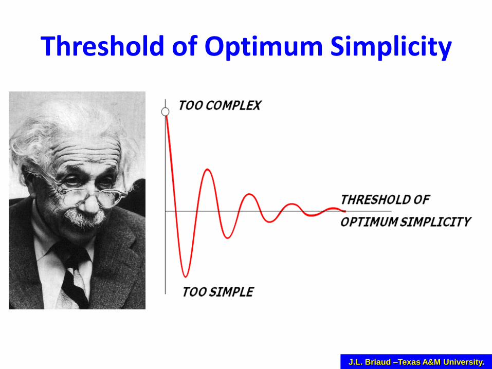
Threshold of Optimum Simplicity
J.L. Briaud –Texas A&M University.
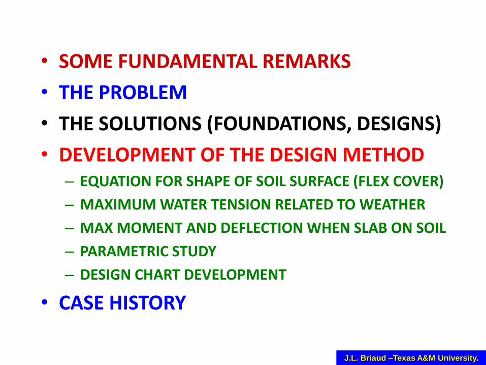
• SOME FUNDAMENTAL REMARKS
• THE PROBLEM
• THE SOLUTIONS (FOUNDATIONS, DESIGNS)
• DEVELOPMENT OF THE DESIGN METHOD– EQUATION FOR SHAPE OF SOIL SURFACE (FLEX COVER)
– MAXIMUM WATER TENSION RELATED TO WEATHER
– MAX MOMENT AND DEFLECTION WHEN SLAB ON SOIL
– PARAMETRIC STUDY
– DESIGN CHART DEVELOPMENT
• CASE HISTORY

J.L. Briaud –Texas A&M University.
Soil State Swell Shrink
Unsaturated Yes No
Saturated Yes Yes
Saturated No Yes
GWL
THE THREE ZONES

J.L. Briaud –Texas A&M University.
WATER NORMAL STRESS
TENSION COMPRESSION
0
(SUCTION)
(pF )
uw (kPa)
(PORE PRESSURE)
J.L. Briaud –Texas A&M University.
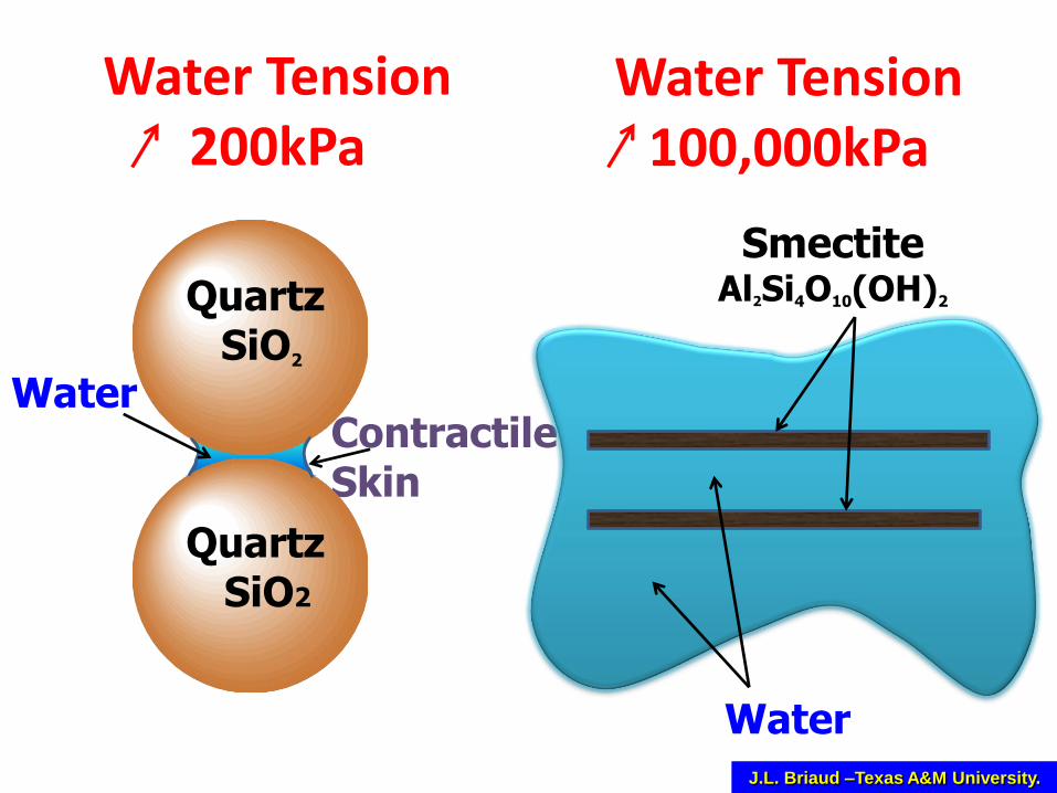
Water Tension 200kPa
Water Tension 100,000kPa
WaterContractile Skin
SmectiteAl2Si4O10(OH)2
Water
QuartzSiO2
QuartzSiO2
J.L. Briaud –Texas A&M University.
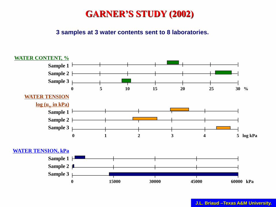
GARNER’S STUDY (2002)
3 samples at 3 water contents sent to 8 laboratories.
WATER CONTENT, %
Sample 1
Sample 2
Sample 3
WATER TENSION
log (uw in kPa)
Sample 1
Sample 2
Sample 3
WATER TENSION, kPa
Sample 1
Sample 2
Sample 3
0 5 10 15 20 25 30 %
0 1 2 3 4 5 log kPa
0 15000 30000 45000 60000 kPa
J.L. Briaud –Texas A&M University.
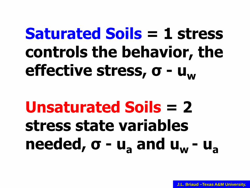
Saturated Soils = 1 stress controls the behavior, theeffective stress, σ - uw
Unsaturated Soils = 2 stress state variables needed, σ - ua and uw - ua
J.L. Briaud –Texas A&M University.
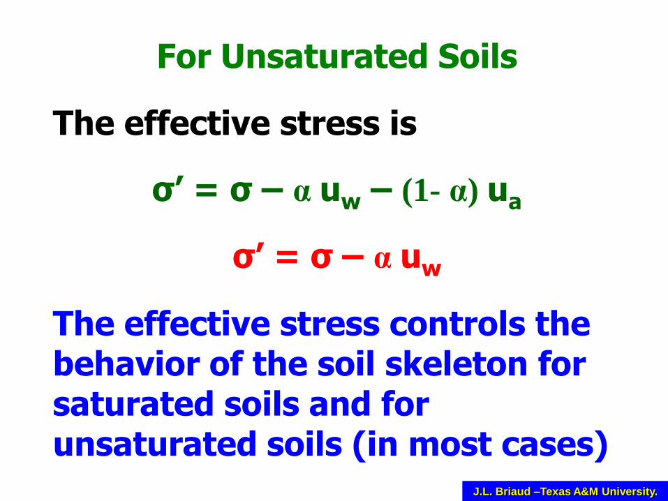
For Unsaturated Soils
The effective stress is
σ’ = σ – α uw – (1- α) ua
σ’ = σ – α uw
The effective stress controls the behavior of the soil skeleton for saturated soils and for unsaturated soils (in most cases)

J.L. Briaud –Texas A&M University.

J.L. Briaud –Texas A&M University.
w
wSW
DV/V
wSH
0
gw/gdShrink-Swell
Index1

J.L. Briaud –Texas A&M University.
CLASSIFICATION OF SHRINK-SWELL POTENTIAL
ACCORDING TO SHRINK-SWELL INDEX
Potential
Very High
High
Moderate
Low
Iss
> 60%
40 – 60
20 – 40
< 20%
J.L. Briaud –Texas A&M University.13
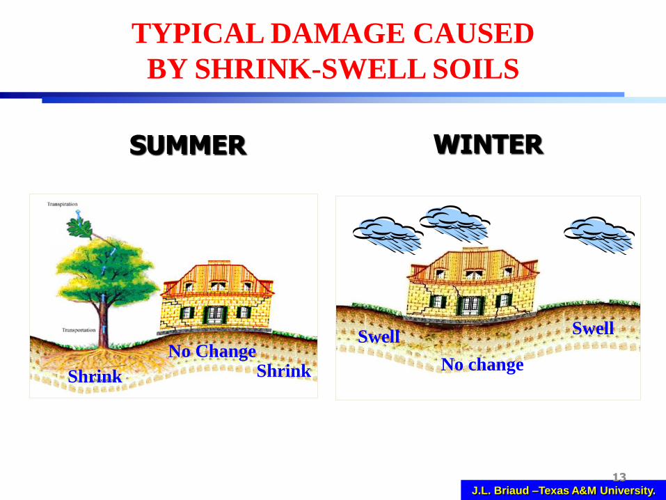
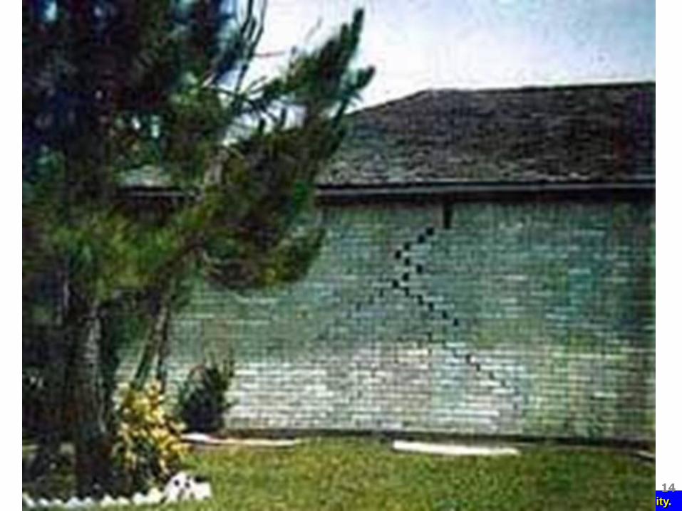
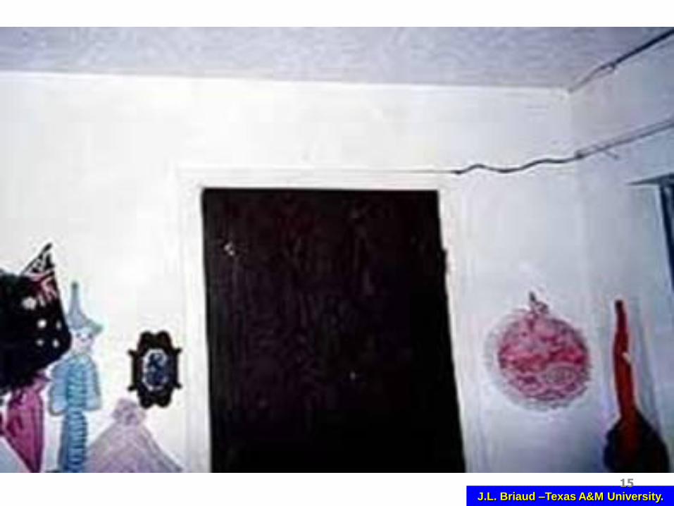
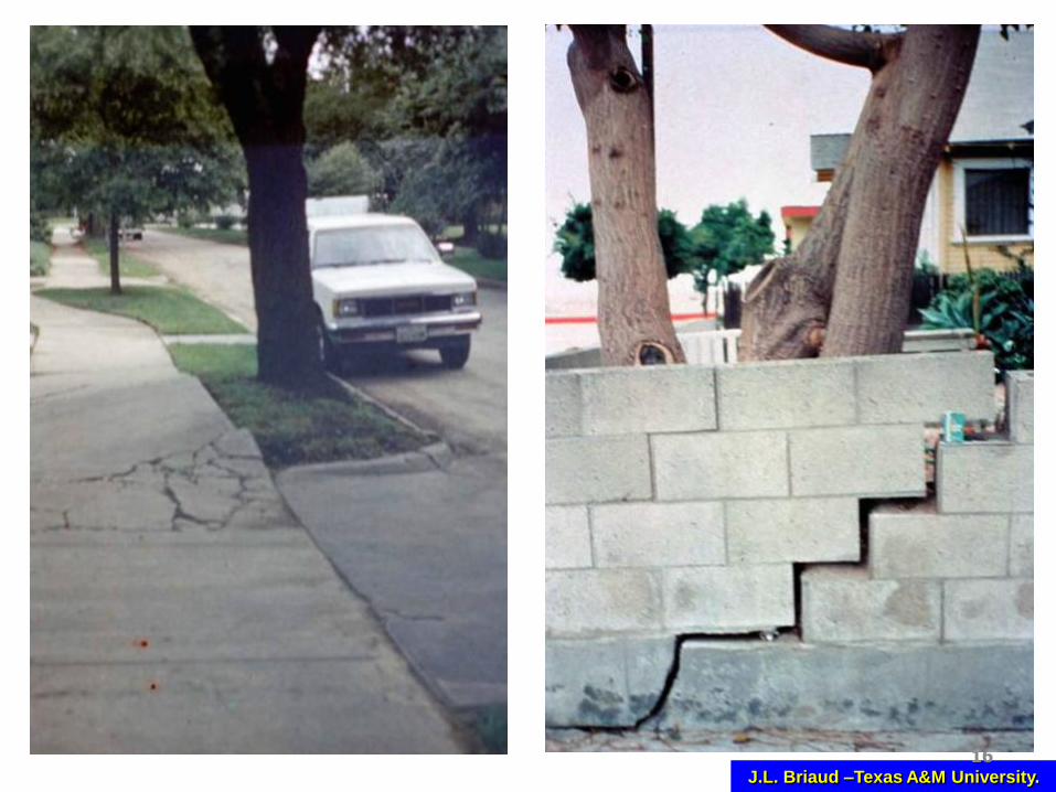
TYPICAL DAMAGE CAUSED
BY SHRINK-SWELL SOILS
SUMMER WINTER
SwellSwell
No changeNo Change
Shrink Shrink
J.L. Briaud –Texas A&M University.14
J.L. Briaud –Texas A&M University.15
J.L. Briaud –Texas A&M University.16

J.L. Briaud –Texas A&M University.17

18
FOUNDATION SOLUTIONS
air gap
• Stiffened Slab on Grade
• Elevated Structural Slab on Piers
• Stiffened Slab on Grade and on Piers
• Thin Post Tensioned Slab

J.L. Briaud –Texas A&M University.
SOME DESIGN METHODS FOR
SLAB-ON-GROUND ON
SHRINK-SWELL SOILS
• BRAB (1968)
• Lytton (1970, 1972, 1973)
• Walsh (1974, 1978)
• Swinburne (1980)
• PTI (1980, 1996, 2004)
• AS 2870 (1980, 1996)
• WRI (1981, 1996)

J.L. Briaud –Texas A&M University.20
..
.
Tributary Load Area
..
.0
.
.0 0
.
.0 0
.
.
Leqv
Leqv

J.L. Briaud –Texas A&M University.21
Q (kN/m)
Mmax
Leqv Δ = f ( Q, EI, L)
EI
Tolerable Distortion
Δ / L = 1/480 Edge drop
Δ / L = 1/960 Edge liftACI 302
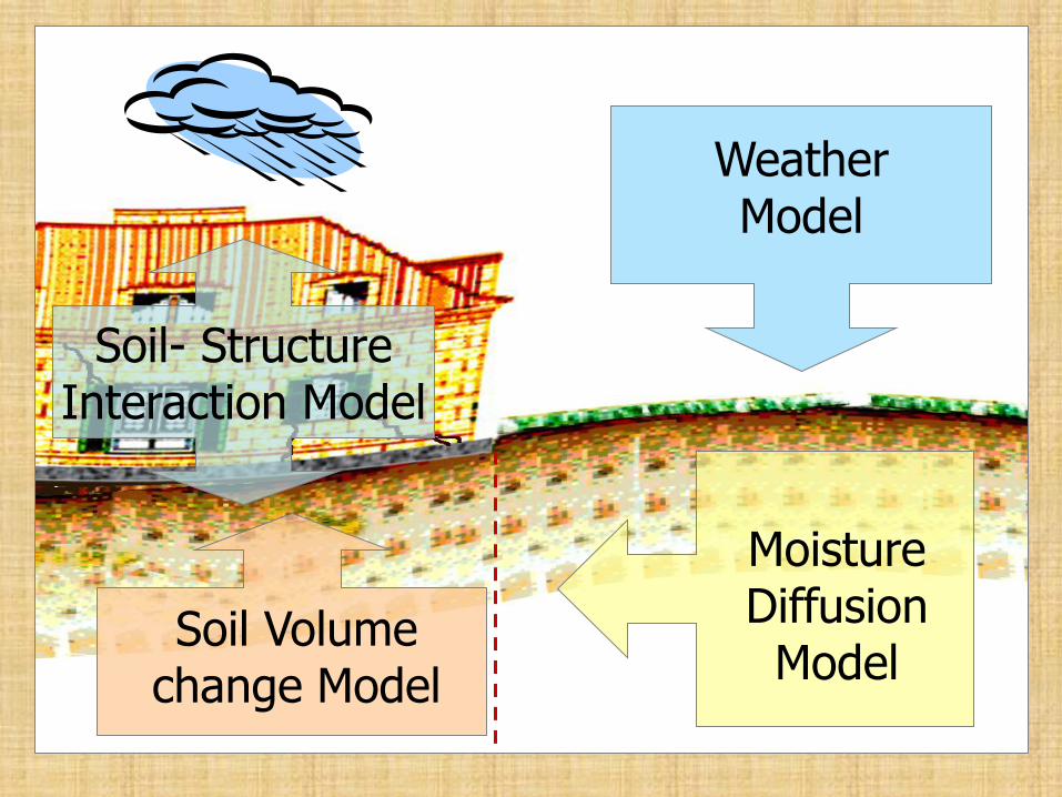
Weather Model
Moisture Diffusion Model
Soil Volume change Model
Soil- Structure Interaction Model

J.L. Briaud –Texas A&M University.
1. Develop a realistic shape of the soil mound partially covered by a flexible cover, function of ΔlogUff
2. Simulate the effect of the weather for 6 cities over a 20 year period to get ΔlogUff.
3. Place the foundation on top of that mound, and obtain Mmax and Δmax
4. Perform an extensive parametric study to find the most important parameters
5. Develop simple design charts based on the results of tasks 1 through 4 to obtain the beam depth and the beam spacing without having to use a computer
DEVELOPMENT OF THE METHOD

VARARIATION OF WATER TENSION
WITH DEPTH
DU(zmax) = 0.1 2DU0
Tension, U
Dep
th, z
Ue0
zmax
U(z,t)
DU0DU0
After Mitchell (1979)
2
2
10log w
U U
t z
U u
J.L. Briaud –Texas A&M University.25
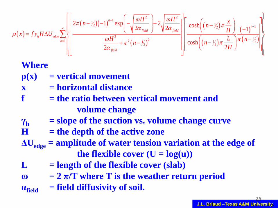
Where
ρ(x) = vertical movement
x = horizontal distance
f = the ratio between vertical movement and
volume change
γh = slope of the suction vs. volume change curve
H = the depth of the active zone
ΔUedge = amplitude of water tension variation at the edge of
the flexible cover (U = log(u))
L = length of the flexible cover (slab)
ω = 2 π/T where T is the weather return period
αfield = field diffusivity of soil.
2 21
112 12
2 1221 21122
2 1 exp 2 cosh2 2 1
cosh22
n
nfield field
h edge
n
field
H H xn nH
x f H ULH n
nnH
g
D

J.L. Briaud –Texas A&M University.26
Developed a procedure to include the influence of the cracks
in the field on the value of alpha in the lab.
β = ratio of crack depth over depth of active zone (Hact)
FCrkDif = ratio of field diffusivity over lab diffusivity (αlab)
To = weather return period
Cracked Soil Diffusion Factor
0
10
20
30
40
50
60
70
1.00E-04 1.00E-03 1.00E-02 1.00E-01 1.00E+00
lab T0 / Hact2
FC
rkD
if
Beta = 0.6667
Beta= 0.80
Beta = 0.5
Influence of cracks is minimum
when diffusivity
is very largeor very small

J.L. Briaud –Texas A&M University.27
Ran 18 simulations of weatherfor 6 cities and
for 20 years each to get the change in water tension Δuff and Δuedge
at the ground surfaceusing the FAO-56 methodology
m
y
y
x
1.5
L
L0.5L
40 Columns of equal
width elements20 Columns of elements with
bias 1.1
25 C
olum
ns o
f el
emen
ts w
ith
bias
1.1
Edge Drop Mound
Cen
ter
Lin
e (
Lin
e of
sym
met
ry)
Foundation slab
ΔuedgeΔuff

J.L. Briaud –Texas A&M University.28
Osborne (1999)

29
Current available methods
Temperature (Thornthwaite, MBC) temp only
Radiation (MMBC, Harg, Turc) temp + radiation
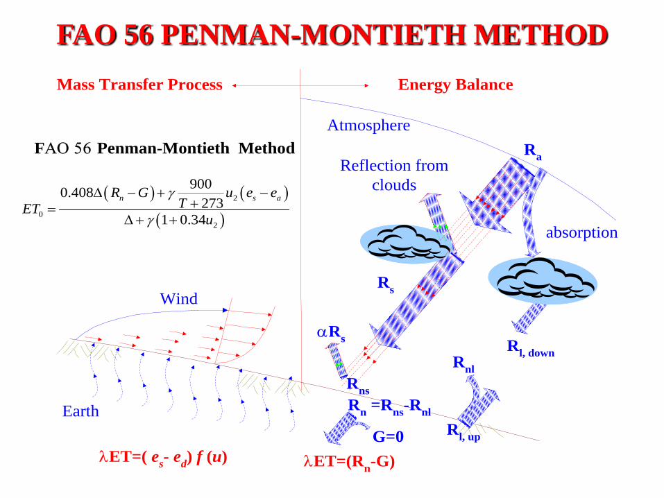
Combination ( FAO 56 PM, ASCE2000 PM) many factors
FAO 56 Penman-Monteith method
International standard, globally valid
Can use daily or hourly weather data
EVAPOTRANSPIRATION METHODS
J.L. Briaud –Texas A&M University.30
FAO 56 PENMAN-MONTIETH METHOD
Ra
Rs
Rs
Rns
Rnl
Rn =R
ns-R
nlEarth
G=0
ET=(Rn-G)
absorption
Reflection from
clouds
Wind
Mass Transfer Process Energy Balance
Atmosphere
ET=( es- e
d) f (u)
Rl, down
Rl, up
2
0
2
9000.408
273
1 0.34
n s aR G u e eTET
u
g
g
D
D
FPenman-Montieth Method
31
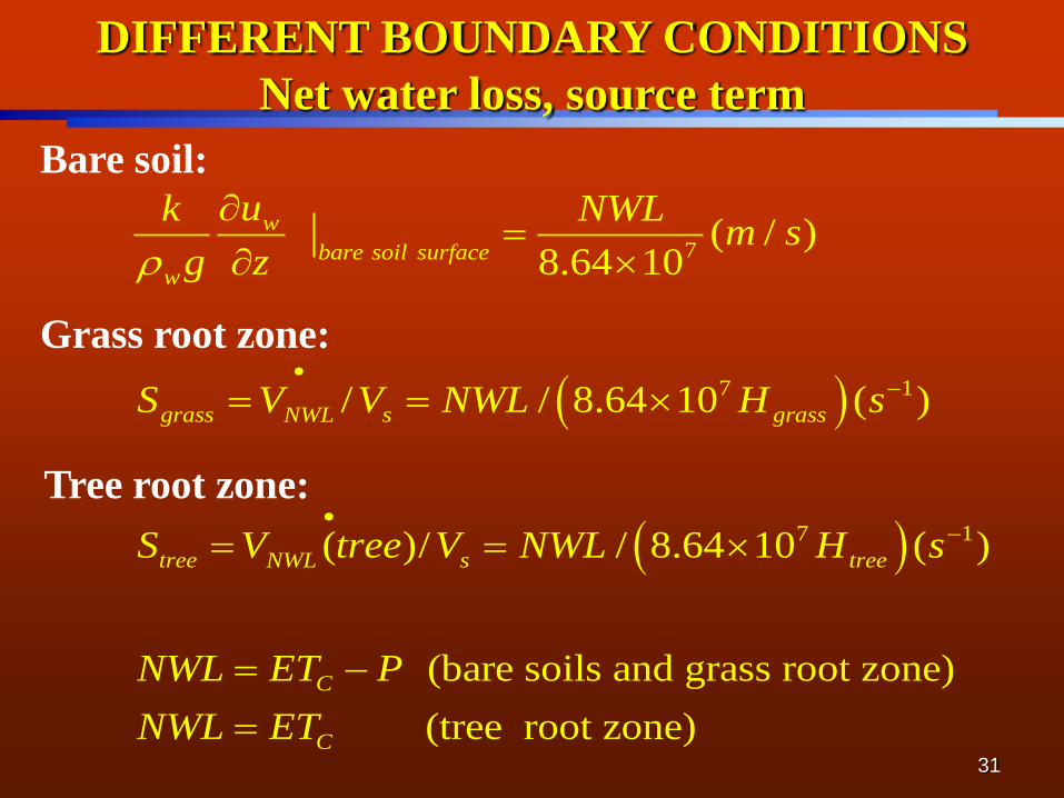
7
7 1
7 1
( / )8.64 10
/ / 8.64 10 ( )
( )/ / 8.64 10 ( )
(bare soils and grass root zone)
w
bare soil surfacew
grass NWL s grass
tree NWL s tree
C
uk NWLm s
g z
S V V NWL H s
S V tree V NWL H s
NWL ET P
(tree root zone) CNWL ET
DIFFERENT BOUNDARY CONDITIONS
Net water loss, source term
Bare soil:
Grass root zone:
Tree root zone:
J.L. Briaud –Texas A&M University.32
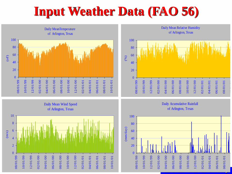
Daily MeanTemperature
of Arlington, Texas
0
20
40
60
80
100
08
/01
/99
10
/01
/99
12
/01
/99
02
/01
/00
04
/01
/00
06
/01
/00
08
/01
/00
10
/01
/00
12
/01
/00
02
/01
/01
04
/01
/01
06
/01
/01
08
/01
/01
10
/01
/01
(oF
)
Daily Mean Relative Humidity
of Arlington, Texas
0
20
40
60
80
100
08
/01
/99
10
/01
/99
12
/01
/99
02
/01
/00
04
/01
/00
06
/01
/00
08
/01
/00
10
/01
/00
12
/01
/00
02
/01
/01
04
/01
/01
06
/01
/01
08
/01
/01
10
/01
/01
(%
)
Daily Mean Wind Speed
of Arlington, Texas
0
2
4
6
8
10
08
/01
/99
10
/01
/99
12
/01
/99
02
/01
/00
04
/01
/00
06
/01
/00
08
/01
/00
10
/01
/00
12
/01
/00
02
/01
/01
04
/01
/01
06
/01
/01
08
/01
/01
10
/01
/01
(m/s
)
Daily Acumulative Rainfall
of Arlington, Texas
0
20
40
60
80
100
08
/01
/99
10
/01
/99
12
/01
/99
02
/01
/00
04
/01
/00
06
/01
/00
08
/01
/00
10
/01
/00
12
/01
/00
02
/01
/01
04
/01
/01
06
/01
/01
08
/01
/01
10
/01
/01
(mm
/day
)
Input Weather Data (FAO 56)

J.L. Briaud –Texas A&M University.
Weather DlogUff(kPa) 1.392 0.788 1.283
Soil-weather
H (m) 3.3 2.4 1.8
Soil ISS (%) 60 45 30
StructuralDimensions
(m)12X12 24X24 24X12
College
Station
TX
San
Antonio
TX
Austin
TX
Dallas
TX
Houston
TX
Denver
CO
DlogUff(kPa) 0.788 1.392 0.866 1.295 1.283 1.374
DlogUedge(kPa) 0.394 0.696 0.433 0.648 0.642 0.687
J.L. Briaud –Texas A&M University.
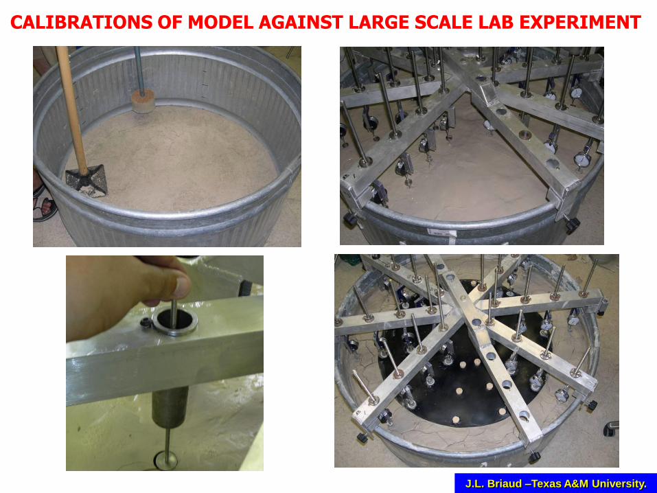
CALIBRATIONS OF MODEL AGAINST LARGE SCALE LAB EXPERIMENT
J.L. Briaud –Texas A&M University.
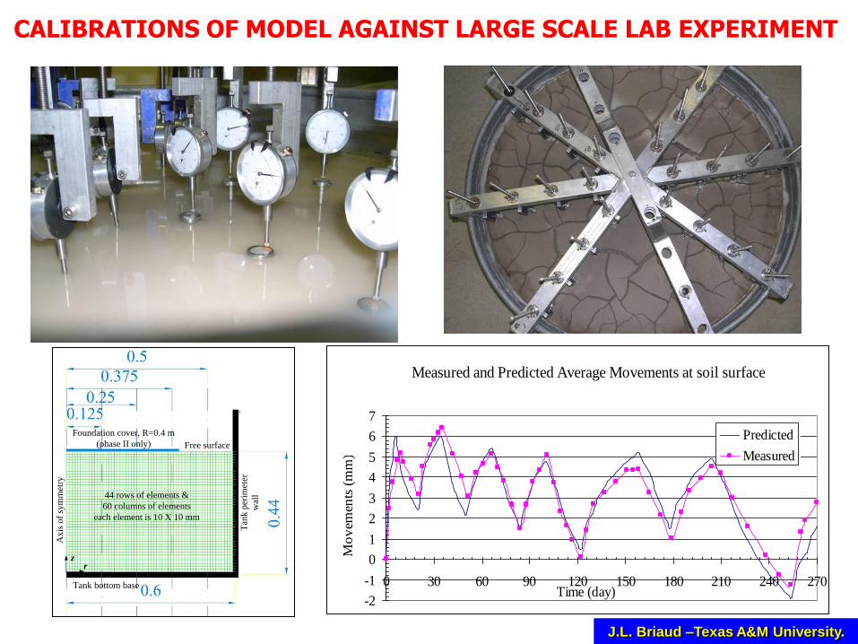
CALIBRATIONS OF MODEL AGAINST LARGE SCALE LAB EXPERIMENT
44 rows of elements &
60 columns of elements
each element is 10 X 10 mm
Foundation cover, R=0.4 m
(phase II only)
zr
Ax
is o
f sy
mm
etry
Tank bottom base
Tan
k p
erim
eter
wal
l
Free surface
Measured and Predicted Average Movements at soil surface
-2
-1
0
1
2
3
4
5
6
7
0 30 60 90 120 150 180 210 240 270Time (day)
Mo
vem
ents
(m
m)
Predicted
Measured
J.L. Briaud –Texas A&M University.
m
y
y
x
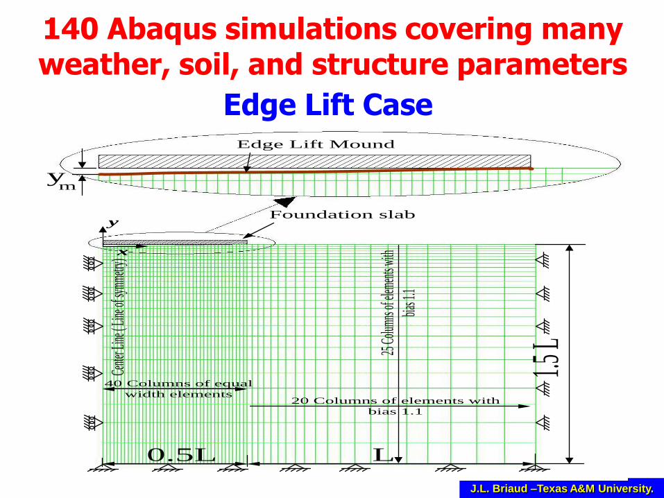
1.5 L
L0.5L
40 Columns of equal
width elements20 Columns of elements with
bias 1.1
25 C
olumn
s of e
lemen
ts wi
th
bias 1
.1
Edge Lift Mound
Cente
r Line
( Line
of sy
mmetr
y)
Foundation slab
Edge Lift Case
140 Abaqus simulations covering manyweather, soil, and structure parameters
J.L. Briaud –Texas A&M University.
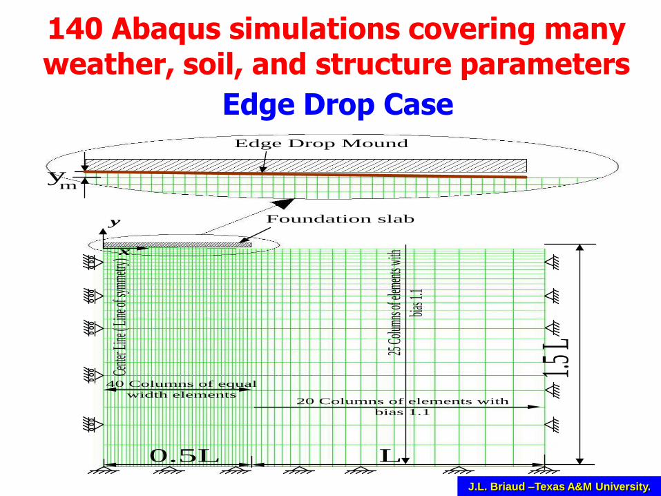
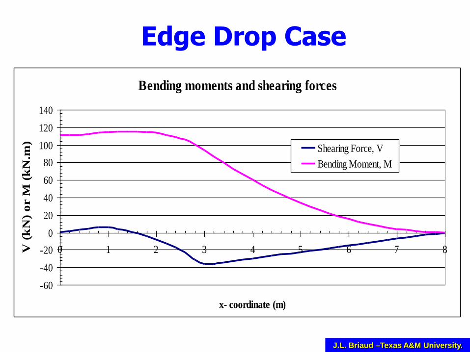
Edge Drop Case
140 Abaqus simulations covering manyweather, soil, and structure parameters
m
y
y
x
1.5 L
L0.5L
40 Columns of equal
width elements20 Columns of elements with
bias 1.1
25 C
olumn
s of e
lemen
ts wi
th
bias 1
.1
Edge Drop Mound
Cente
r Line
( Line
of sy
mmetr
y)
Foundation slab

J.L. Briaud –Texas A&M University.
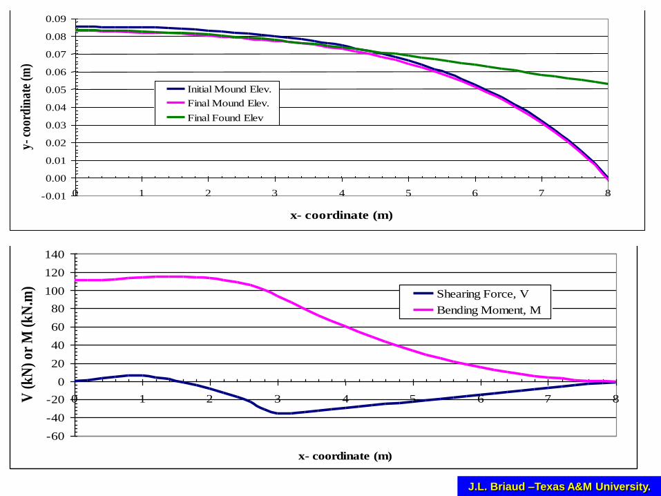
Soil mound and foundation elevations
-0.01
0.00
0.01
0.02
0.03
0.04
0.05
0.06
0.07
0.08
0.09
0 1 2 3 4 5 6 7 8
x- coordinate (m)
y-
co
ord
ina
te (
m)
Initial Mound Elev.
Final Mound Elev.
Final Found Elev
Edge Drop Case
J.L. Briaud –Texas A&M University.
Bending moments and shearing forces
-60
-40
-20
0
20
40
60
80
100
120
140
0 1 2 3 4 5 6 7 8
x- coordinate (m)
V (
kN
) o
r M
(k
N.m
)
Shearing Force, V
Bending Moment, M
Edge Drop Case
J.L. Briaud –Texas A&M University.
Soil mound and foundation elevations
-0.01
0.00
0.01
0.02
0.03
0.04
0.05
0.06
0.07
0.08
0.09
0 1 2 3 4 5 6 7 8
x- coordinate (m)
y- c
oord
inat
e (m
)
Initial Mound Elev.
Final Mound Elev.
Final Found Elev
Bending moments and shearing forces
-60
-40
-20
0
20
40
60
80
100
120
140
0 1 2 3 4 5 6 7 8
x- coordinate (m)
V (
kN
) or
M (
kN
.m)
Shearing Force, V
Bending Moment, M
J.L. Briaud –Texas A&M University.41
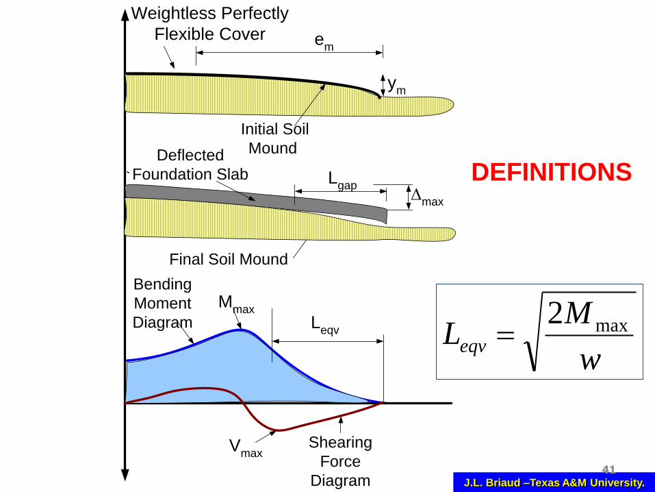
w
MLeqv
max2
Bending
Moment
Diagram
Shearing
Force
Diagram
Mmax
Vmax
Weightless Perfectly
Flexible Cover
Initial Soil
Mound
ym
em
Deflected
Foundation Slab Lgap
Leqv
Final Soil Mound
Dmax
DEFINITIONS

J.L. Briaud –Texas A&M University.
IS-W Comment Iss (%) H (m) DU0 (pF) D (m) L (m) wimposed (kPa)
0 No mound 45 3.5 0 0.9 16 3.5
2.0475 reference 45 3.5 1.3 0.9 16 3.5
3.4125 Iss- Very High 75 3.5 1.3 0.9 16 3.5
2.73 Iss- High 60 3.5 1.3 0.9 16 3.5
1.365 Iss- Moderate 30 3.5 1.3 0.9 16 3.5
0.6825 Iss- Low 15 3.5 1.3 0.9 16 3.5
3.2175 H- Very High 45 5.5 1.3 0.9 16 3.5
2.6325 H- High 45 4.5 1.3 0.9 16 3.5
1.4625 H- Moderate 45 2.5 1.3 0.9 16 3.5
0.8775 H- Low 45 1.5 1.3 0.9 16 3.5
2.52 DU-Very High 45 3.5 1.6 0.9 16 3.5
2.28375 DU-High 45 3.5 1.45 0.9 16 3.5
1.81125 DU-Moderate 45 3.5 1.15 0.9 16 3.5
1.575 DU-Low 45 3.5 1 0.9 16 3.5
2.0475 wimposed-Very High 45 3.5 1.3 0.9 16 5
2.0475 wimposed -High 45 3.5 1.3 0.9 16 4.25
2.0475 wimposed-Moderate 45 3.5 1.3 0.9 16 2.75
2.0475 wimposed-Low 45 3.5 1.3 0.9 16 2
6.6 All maximums 75 5.5 1.6 0.9 16 3.5
0.225 All minimums 15 1.5 1 0.9 16 3.5
DlogUff

J.L. Briaud –Texas A&M University.
Influence of soil shrink-swell potential on Leqv
0
0.2
0.4
0.6
0.8
1
1.2
1.4
0 0.5 1 1.5 2
Normalized Iss ( Iss / Iss (reference case))
No
rmal
ized
Leq
v
(Leq
v/
Leq
v (
refe
ren
ce c
ase
))
Edge drop case
Edge lift case
Influence of soil surface suction change on Leqv
0
0.2
0.4
0.6
0.8
1
1.2
0 0.2 0.4 0.6 0.8 1 1.2 1.4
Normalized DU0 ( DU0 / DU0 (reference case))
No
rmal
ized
Leq
v
(Leq
v/
Leq
v (
refe
ren
ce c
ase)
)
Edge drop case
Edge lift case
Influence of slab beam depth on Leqv
0
0.2
0.4
0.6
0.8
1
1.2
1.4
1.6
0 0.5 1 1.5 2
Normalized D ( D / D (reference case))
No
rmal
ized
Leq
v
(Leq
v/
Leq
v (
refe
ren
ce c
ase
))
Edge drop case
Edge lift case
Influence of slab imposed loads on Leqv
0
0.2
0.4
0.6
0.8
1
1.2
0 0.5 1 1.5
Normalized wimposed ( wimposed / wimposed (reference case))
No
rmal
ized
Leq
v
(Leq
v/
Leq
v (
refe
ren
ce c
ase
))Edge drop case
Edge lift case
Influence of slab length on Leqv
0
0.2
0.4
0.6
0.8
1
1.2
0 1 2 3 4
Normalized L ( L / 2H (reference case))
No
rmal
ized
Leq
v
(Leq
v/
Leq
v (
refe
ren
ce c
ase
))
Edge drop case
Edge lift case
Influence of depth of active moisture zone on Leqv
0
0.2
0.4
0.6
0.8
1
1.2
1.4
0 0.5 1 1.5 2
Normalized H ( H / H (reference case))
No
rmal
ized
Leq
v
(Leq
v/
Leq
v (
refe
ren
ce c
ase
))
Edge drop case
Edge lift case
Leqv
as a f()of
Iss
ΔlogUff
HDLw
J.L. Briaud –Texas A&M University.
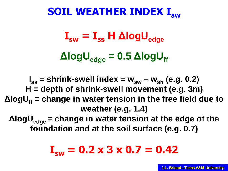
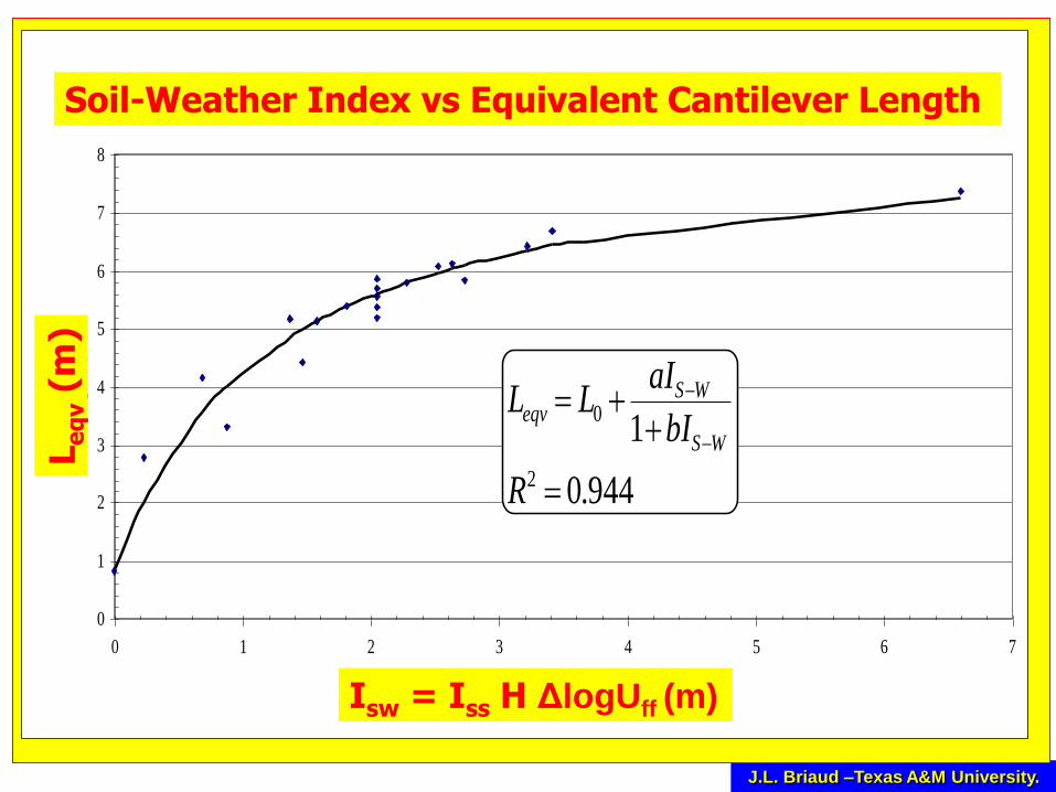
SOIL WEATHER INDEX Isw
Isw = Iss H ΔlogUedge
ΔlogUedge = 0.5 ΔlogUff
Iss = shrink-swell index = wsw – wsh (e.g. 0.2)
H = depth of shrink-swell movement (e.g. 3m)
ΔlogUff = change in water tension in the free field due to
weather (e.g. 1.4)
ΔlogUedge = change in water tension at the edge of the
foundation and at the soil surface (e.g. 0.7)
Isw = 0.2 x 3 x 0.7 = 0.42
J.L. Briaud –Texas A&M University.
Soil-Weather Index versus Equivalent cantilever length.
0
1
2
3
4
5
6
7
8
0 1 2 3 4 5 6 7
Iss H DU0 (m)
Leqv. (m
)
944.0
12
0
R
bI
aILL
WS
WSeqv
Isw = Iss H ΔlogUff (m)
Le
qv
(m)
Soil-Weather Index vs Equivalent Cantilever Length
J.L. Briaud –Texas A&M University.46
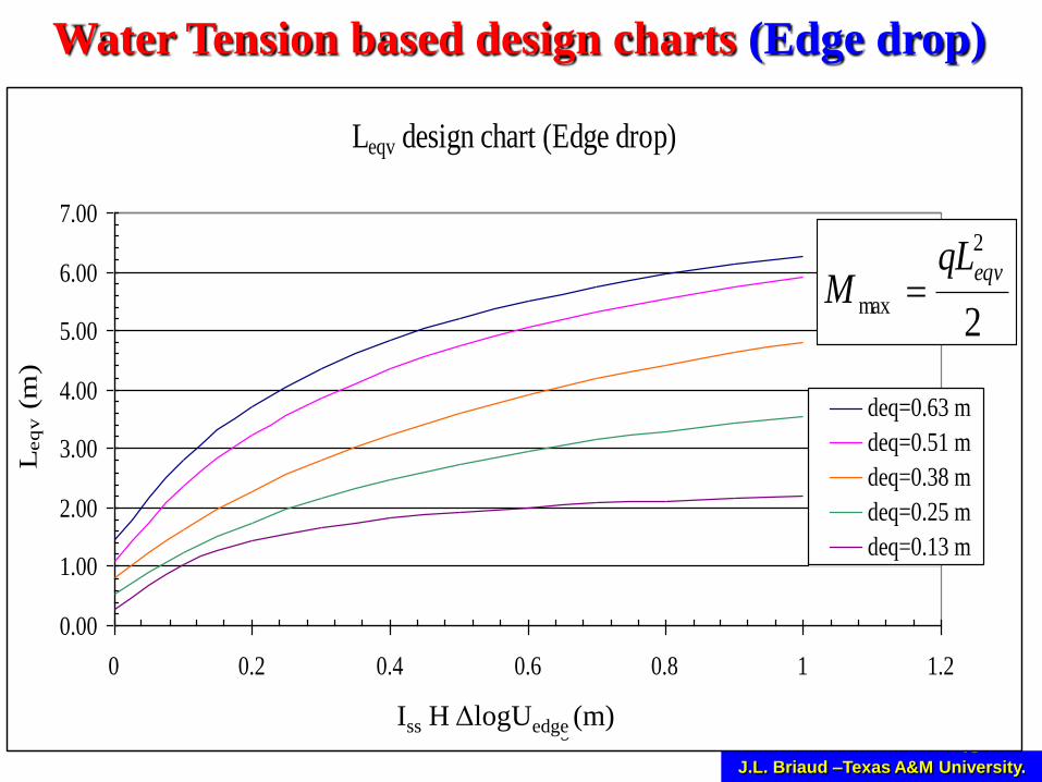
Water Tension based design charts (Edge drop)
Leqv design chart (Edge drop)
0.00
1.00
2.00
3.00
4.00
5.00
6.00
7.00
0 0.2 0.4 0.6 0.8 1 1.2
Iss. H. DUedge (m)
Leq
v (
m)
deq=0.63 m
deq=0.51 m
deq=0.38 m
deq=0.25 m
deq=0.13 m
2
2
max
eqvqLM
Iss H ΔlogUedge (m)

J.L. Briaud –Texas A&M University.47
Lgap design chart (Edge drop)
0.00
0.50
1.00
1.50
2.00
2.50
3.00
3.50
4.00
4.50
5.00
0 0.2 0.4 0.6 0.8 1 1.2
Iss. H. DUedge (m)
Lg
ap (
m)
deq=0.63 m
deq=0.51 m
deq=0.38 m
deq=0.25 m
deq=0.13 m
Water Tension based design charts (Edge drop)
Iss H ΔlogUedge (m)

J.L. Briaud –Texas A&M University.48
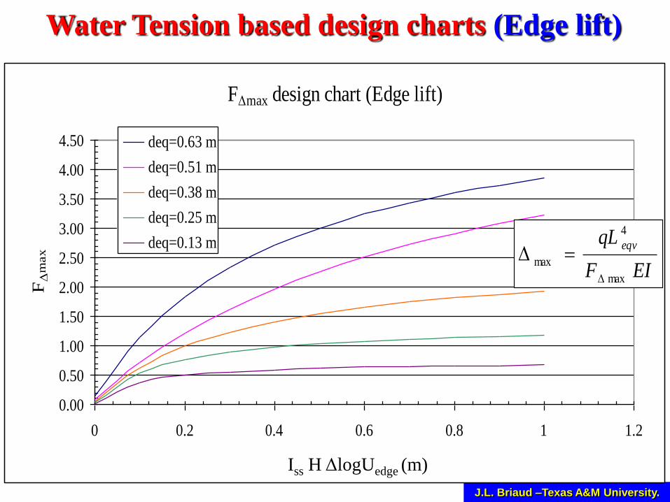
FDmax design chart (Edge drop)
0.00
0.50
1.00
1.50
2.00
2.50
3.00
3.50
4.00
4.50
0 0.2 0.4 0.6 0.8 1 1.2
Iss. H. DUedge (m)
FD
max
deq=0.63 m
deq=0.51 m
deq=0.38 m
deq=0.25 m
deq=0.13 m
EIF
qL eqv
max
4
max
D
D
Water Tension based design charts (Edge drop)
Iss H ΔlogUedge (m)
J.L. Briaud –Texas A&M University.49
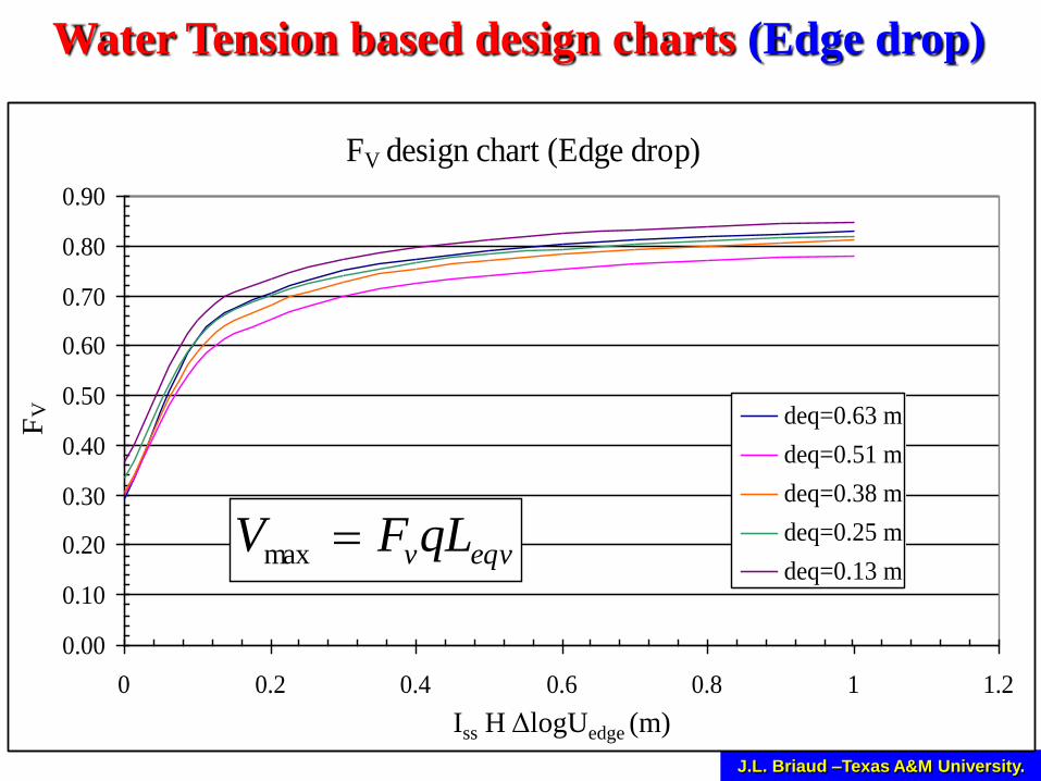
FV design chart (Edge drop)
0.00
0.10
0.20
0.30
0.40
0.50
0.60
0.70
0.80
0.90
0 0.2 0.4 0.6 0.8 1 1.2
Iss. H. DUedge (m)
FV
deq=0.63 m
deq=0.51 m
deq=0.38 m
deq=0.25 m
deq=0.13 meqvvqLFV max
Water Tension based design charts (Edge drop)
Iss H ΔlogUedge (m)

J.L. Briaud –Texas A&M University.50
Leqv design chart (Edge lift)
0.00
1.00
2.00
3.00
4.00
5.00
6.00
7.00
8.00
0 0.2 0.4 0.6 0.8 1 1.2
Iss. H. DUedge (m)
Leq
v (
m)
deq=0.63 m
deq=0.51 m
deq=0.38 m
deq=0.25 m
deq=0.13 m
2
2
max
eqvqLM
Water Tension based design charts (Edge lift)
Iss H ΔlogUedge (m)
J.L. Briaud –Texas A&M University.51
FDmax design chart (Edge lift)
0.00
0.50
1.00
1.50
2.00
2.50
3.00
3.50
4.00
4.50
0 0.2 0.4 0.6 0.8 1 1.2
Iss. H. DUedge (m)
FD
max
deq=0.63 m
deq=0.51 m
deq=0.38 m
deq=0.25 m
deq=0.13 m
EIF
qL eqv
max
4
max
D
D
Water Tension based design charts (Edge lift)
Iss H ΔlogUedge (m)
J.L. Briaud –Texas A&M University.52
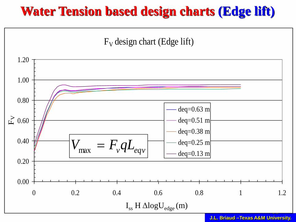
FV design chart (Edge lift)
0.00
0.20
0.40
0.60
0.80
1.00
1.20
0 0.2 0.4 0.6 0.8 1 1.2
Iss. H.DUedge (m)
FV
deq=0.63 m
deq=0.51 m
deq=0.38 m
deq=0.25 m
deq=0.13 meqvvqLFV max
Water Tension based design charts (Edge lift)
Iss H ΔlogUedge (m)

J.L. Briaud –Texas A&M University.
Developed a simple correlation between theSlope of the SWCC Cw and the shrink-swell index Iss.
CW = 0.51 ISS
R2 = 0.889
0
5
10
15
20
25
15 20 25 30 35 40 45
Iss (%)
Cw
(%
)
ThereforeΔwedge = Cw ΔlogUedge = 0.5 Iss ΔlogUedge
Then ISW (for water tension) = ISS H ΔlogUedge = 2 H Δwedge
ISW (for water content) = H Δwedge
ISW (for water tension) = 2 ISW (for water content)
ISS = 0.734 PI
R2 = 0.4965
15
20
25
30
35
40
45
20 25 30 35 40 45 50
PI (%)
I SS
(%)
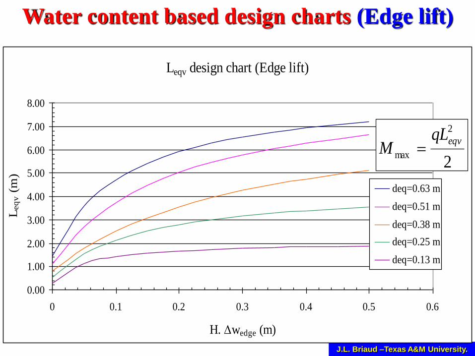
J.L. Briaud –Texas A&M University.54
Leqv design chart (Edge drop)
0.00
1.00
2.00
3.00
4.00
5.00
6.00
7.00
0 0.1 0.2 0.3 0.4 0.5 0.6
H. Dwedge (m)
Leq
v (
m)
deq=0.63 m
deq=0.51 m
deq=0.38 m
deq=0.25 m
deq=0.13 m
2
2
max
eqvqLM
Water content based design charts (Edge drop)

J.L. Briaud –Texas A&M University.55
Lgap design chart (Edge drop)
0.00
0.50
1.00
1.50
2.00
2.50
3.00
3.50
4.00
4.50
5.00
0 0.1 0.2 0.3 0.4 0.5 0.6
H. Dwedge (m)
Lg
ap (
m)
deq=0.63 m
deq=0.51 m
deq=0.38 m
deq=0.25 m
deq=0.13 m
Water content based design charts (Edge drop)

J.L. Briaud –Texas A&M University.56
Water content based design charts (Edge drop)
FDmax design chart (Edge drop)
0.00
0.50
1.00
1.50
2.00
2.50
3.00
3.50
4.00
4.50
0 0.1 0.2 0.3 0.4 0.5 0.6
H. Dwedge (m)
FD
max
deq=0.63 m
deq=0.51 m
deq=0.38 m
deq=0.25 m
deq=0.13 m
EIF
qL eqv
max
4
max
D
D
J.L. Briaud –Texas A&M University.57
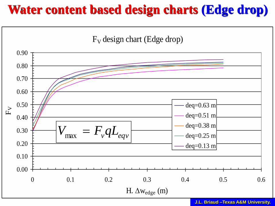
Water content based design charts (Edge drop)
FV design chart (Edge drop)
0.00
0.10
0.20
0.30
0.40
0.50
0.60
0.70
0.80
0.90
0 0.1 0.2 0.3 0.4 0.5 0.6
H. Dwedge (m)
FV
deq=0.63 m
deq=0.51 m
deq=0.38 m
deq=0.25 m
deq=0.13 m
eqvvqLFV max
J.L. Briaud –Texas A&M University.58
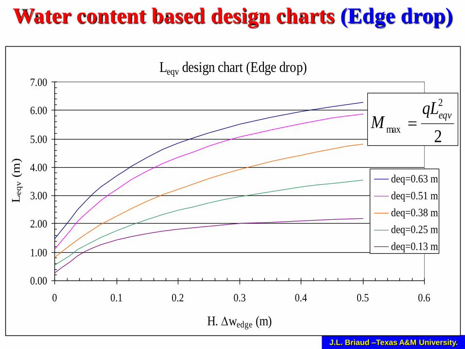
Water content based design charts (Edge lift)
Leqv design chart (Edge lift)
0.00
1.00
2.00
3.00
4.00
5.00
6.00
7.00
8.00
0 0.1 0.2 0.3 0.4 0.5 0.6
H. Dwedge (m)
Leq
v (
m)
deq=0.63 m
deq=0.51 m
deq=0.38 m
deq=0.25 m
deq=0.13 m
2
2
max
eqvqLM

J.L. Briaud –Texas A&M University.59
Water content based design charts (Edge lift)
FDmax design chart (Edge lift)
0.00
0.50
1.00
1.50
2.00
2.50
3.00
3.50
4.00
4.50
0 0.1 0.2 0.3 0.4 0.5 0.6
H. Dwedge (m)
FD
max
deq=0.63 m
deq=0.51 m
deq=0.38 m
deq=0.25 m
deq=0.13 mEIF
qL eqv
max
4
max
D
D

J.L. Briaud –Texas A&M University.60
Water content based design charts (Edge lift)
FV design chart (Edge lift)
0.00
0.20
0.40
0.60
0.80
1.00
1.20
0 0.1 0.2 0.3 0.4 0.5 0.6
H.Dwedge (m)
FV
deq=0.63 m
deq=0.51 m
deq=0.38 m
deq=0.25 m
deq=0.13 m
eqvvqLFV max

J.L. Briaud –Texas A&M University.61
PROPOSED
DESIGN PROCEDURE
1.Water content version: one version of
the method uses the water content of the
soil.
2.Water tension version: one version of
the method uses the water tension in the
soil.

J.L. Briaud –Texas A&M University.62
PROPOSED
DESIGN PROCEDURE
1.Gather site specific information on
active depth and amplitude of water
content or water tension variation at the
foundation level.
2.Use 3 charts to obtain maximum
bending moment, maximum shear force,
and maximum deflection (distortion)
J.L. Briaud –Texas A&M University.
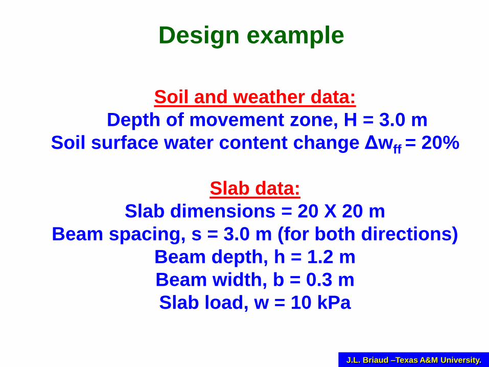
Design example
Soil and weather data:
Depth of movement zone, H = 3.0 m
Soil surface water content change Δwff = 20%
Slab data:
Slab dimensions = 20 X 20 m
Beam spacing, s = 3.0 m (for both directions)
Beam depth, h = 1.2 m
Beam width, b = 0.3 m
Slab load, w = 10 kPa

J.L. Briaud –Texas A&M University.
Soil-Weather Index Is-w
Δwedge = 0.5 Δwff = 0.5 x 0.2 = 0.1 or 10%
Is-w = Δwedge x H = 0.1 x 3 = 0.3 m
Slab bending stiffness
EI = E bh3/12 = 2 x 107 x 0.3 x 1.23 / 12 = 8.64 x 10⁵ kN.m2
Equivalent slab thickness
b h3/12 = s deq3/12
deq = h (b/s)1/3 = 1.2 (0.3/3)1/3 = 0.56 m
Values from charts
Leq = 5.3 m for maximum moment
Lgap = 3.6 m for information
FΔmax = 2.9 for maximum deflection
Fv = 0.8 for maximum shear
J.L. Briaud –Texas A&M University.
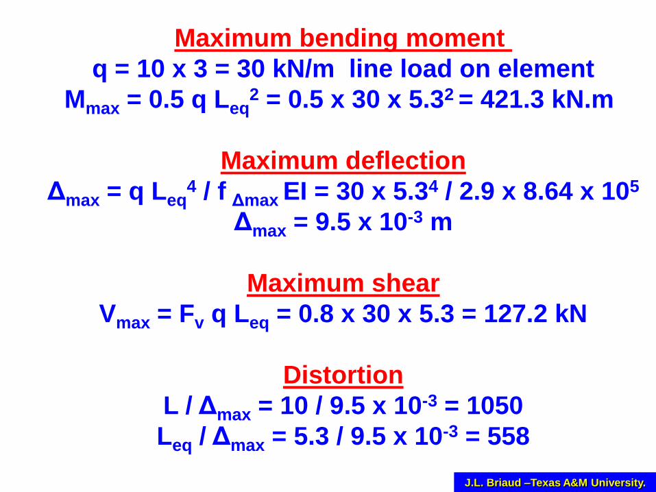
Maximum bending moment
q = 10 x 3 = 30 kN/m line load on element
Mmax = 0.5 q Leq2 = 0.5 x 30 x 5.32 = 421.3 kN.m
Maximum deflection
Δmax = q Leq4 / f Δmax EI = 30 x 5.34 / 2.9 x 8.64 x 105
Δmax = 9.5 x 10⁻³ m
Maximum shear
Vmax = Fv q Leq = 0.8 x 30 x 5.3 = 127.2 kN
Distortion
L / Δmax = 10 / 9.5 x 10-3 = 1050
Leq / Δmax = 5.3 / 9.5 x 10-3 = 558

J.L. Briaud –Texas A&M University.66
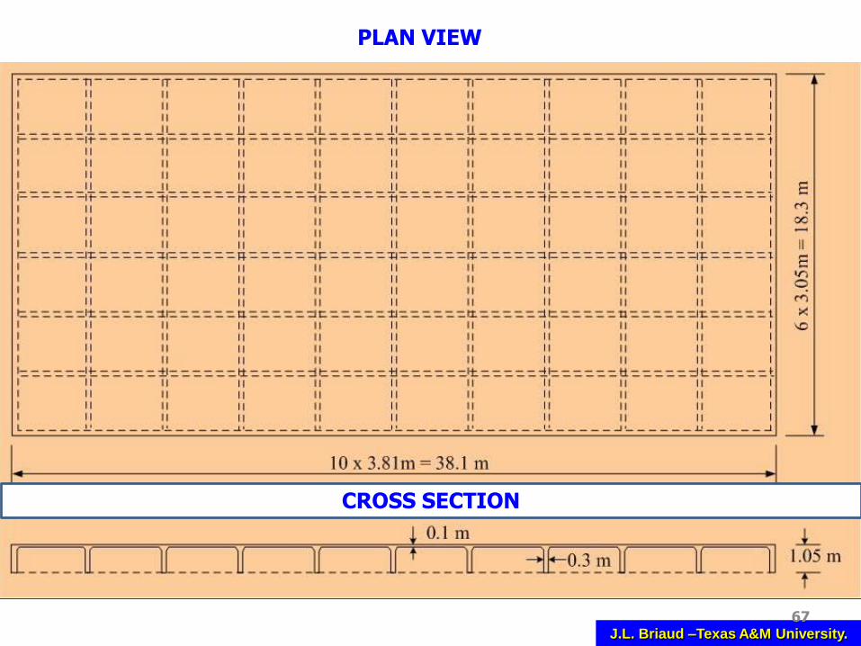
ELLISON BUILDING CASE
STUDY
J.L. Briaud –Texas A&M University.67
CROSS SECTION
PLAN VIEW
J.L. Briaud –Texas A&M University.68
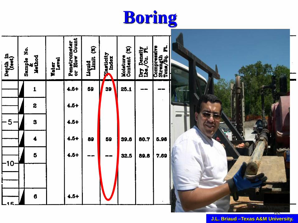
Boring

J.L. Briaud –Texas A&M University.69
Soil properties- Soil type: CH- PL=30%,LL=80%,PI= 50%- Percent clay = 60%- Allowable bearing pres. = 75 kPa- Depth to constant suction = 2.1 m- Modulus of Elasticity = 7000 kPa- Total unit weight = 20 kN/m3
Loads- No interior load- Perimeter loading = 32 kN/m- Live load = 2 kPa
LocationCollege Station, TX, USA
Concrete Slab properties- Compressive Strength = 20 MPa- Creep Modulus = 10000 MPA- Unit Weight = 23 kN/m3
- Beam width = 0.3 m- Slab thickness = 100 mm- Allowable distortion Δ/L=1/500
CASE HISTORY DATA

J.L. Briaud –Texas A&M University.
#4@16" OCEW
0.1 m
1.05 m
3-#6
#3 TIES @ 24" C-C
2-#5
6 MIL POLY
0.3 m
3-#6
70
J.L. Briaud –Texas A&M University.
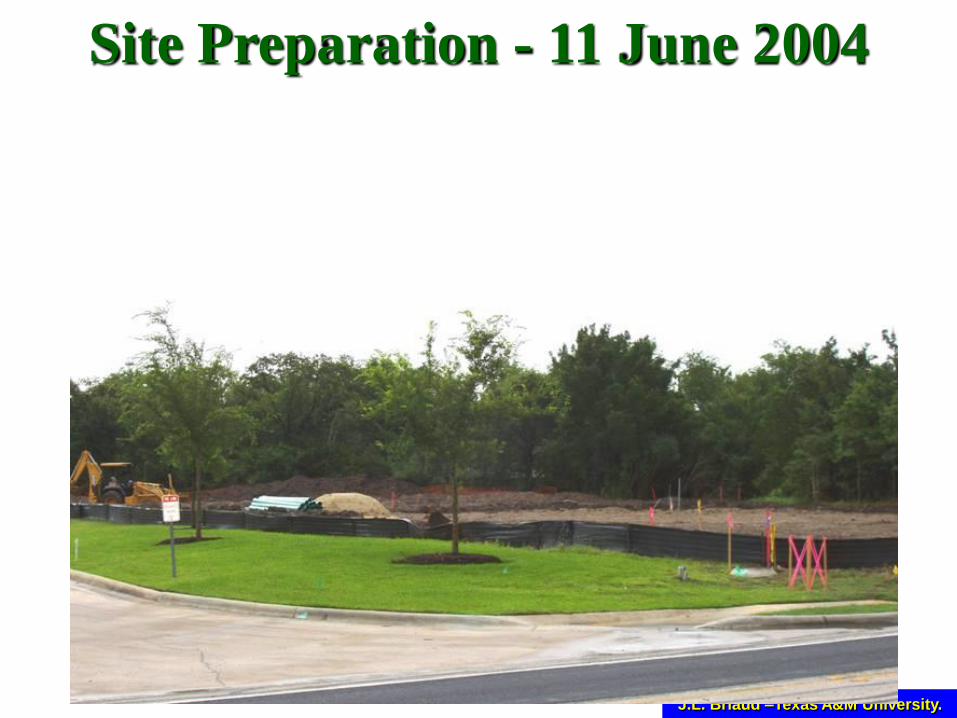
Site Preparation - 11 June 2004
J.L. Briaud –Texas A&M University.
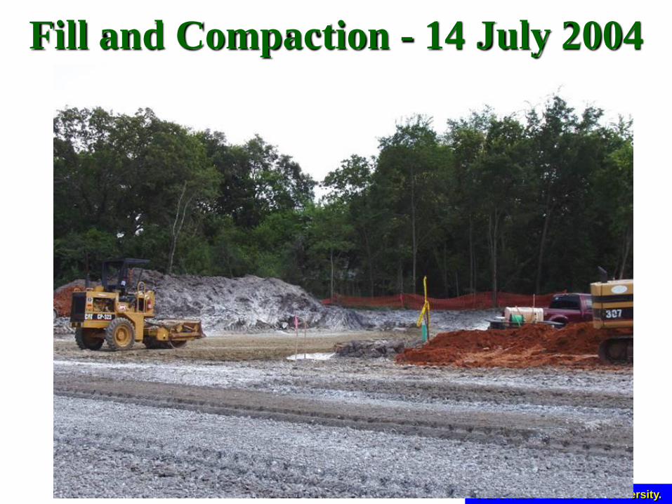
Fill and Compaction - 14 July 2004

J.L. Briaud –Texas A&M University.73
Excavation and steel - 16 July 2004
J.L. Briaud –Texas A&M University.

J.L. Briaud –Texas A&M University.

J.L. Briaud –Texas A&M University.

J.L. Briaud –Texas A&M University.

J.L. Briaud –Texas A&M University.

J.L. Briaud –Texas A&M University.79

J.L. Briaud –Texas A&M University.80
Installing Tell Tales – 13 Aug 2004
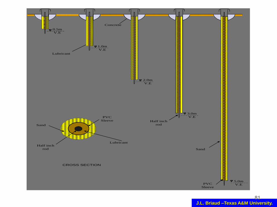
J.L. Briaud –Texas A&M University.81
0.5m
V.E
1.0m
V.E
2.0m
V.E
3.0m
V.E
5.0m
V.E
Lubricant
Concrete
Half inch
rod
Sand
PVC
Sleeve
Half inch
rod
Lubricant
Sand
PVC
Sleeve
CROSS SECTION

J.L. Briaud –Texas A&M University.82
Installing Benchmark - 13Aug 2004

J.L. Briaud –Texas A&M University.83
Installing Slab Bolts – 13 Aug 2004

J.L. Briaud –Texas A&M University.84
Steel Framing - 13-25 Aug 2004

J.L. Briaud –Texas A&M University.85
Wall Construction - Sept 2004
J.L. Briaud –Texas A&M University.
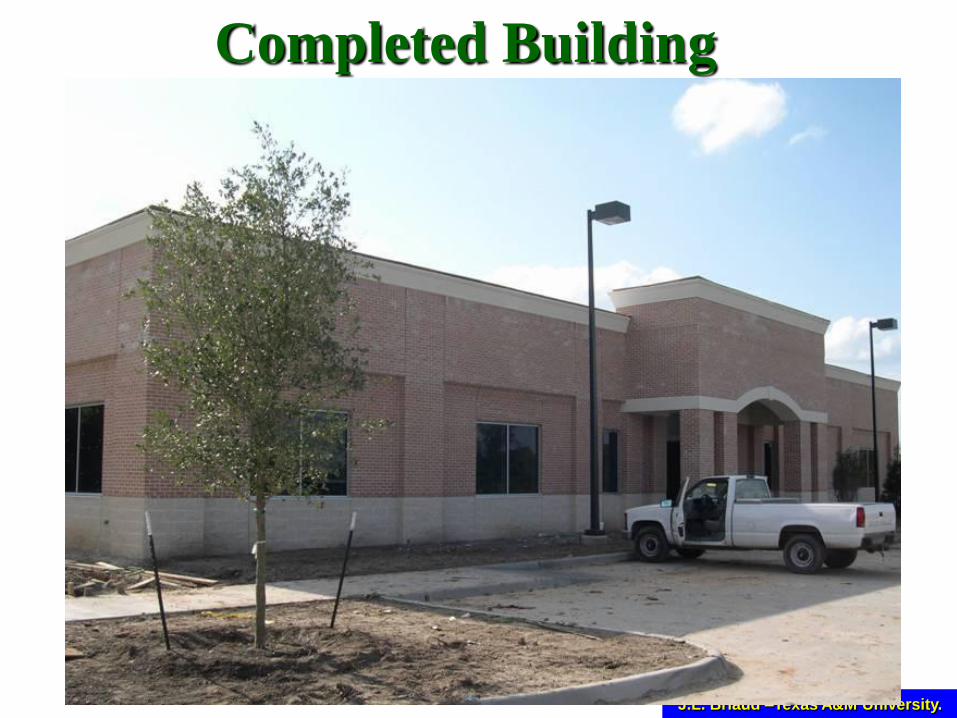
Completed Building

J.L. Briaud –Texas A&M University.87
0.0
4.4
8.9
13.3
17.7
22.2
26.6
31.0
35.4
18.314.2
10.26.1
2.0-0.005
0
0.005
0.01
0.015
0.02
0.025
Elevation (m)
Length (m)
Width (m)
Elevation is referenced to the lowest point on Sept 1, 2004
0.02-0.025
0.015-0.02
0.01-0.015
0.005-0.01
0-0.005
-0.01-0Entrance
INITIAL ELEVATIONS - 1 Sept 2004
J.L. Briaud –Texas A&M University.88
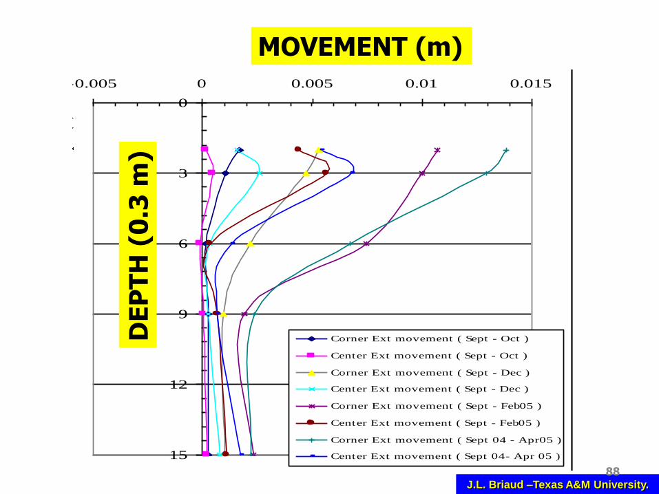
Soil movement log
0
3
6
9
12
15
-0.005 0 0.005 0.01 0.015
Movements (m)D
epth
(ft)
Corner Ext movement ( Sept - Oct )
Center Ext movement ( Sept - Oct )
Corner Ext movement ( Sept - Dec )
Center Ext movement ( Sept - Dec )
Corner Ext movement ( Sept - Feb05 )
Center Ext movement ( Sept - Feb05 )
Corner Ext movement ( Sept 04 - Apr05 )
Center Ext movement ( Sept 04- Apr 05 )
MOVEMENT (m)
DE
PT
H (
0.3
m)

J.L. Briaud –Texas A&M University.89
Perimeter average level vs. Interior average level
-0.003
-0.002
-0.001
0
0.001
0.002
0.003
0.004
0.005
0.006
0.007
0 30 60 90 120 150 180 210 240 270
Time (days)
Re
lati
ve
ele
va
tio
ns
in
(m
)
Perimeter average level
Interior average level
Difference (per-int)
SLAB MOVEMENT over 1 YEAR
J.L. Briaud –Texas A&M University.
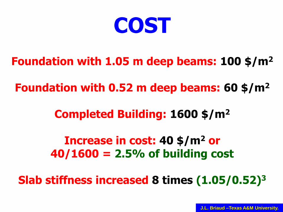
COST
Foundation with 1.05 m deep beams: 100 $/m2
Foundation with 0.52 m deep beams: 60 $/m2
Completed Building: 1600 $/m2
Increase in cost: 40 $/m2 or40/1600 = 2.5% of building cost
Slab stiffness increased 8 times (1.05/0.52)3

J.L. Briaud –Texas A&M University.91
Weather ModelFAO 56
(simulation for different cities)
Soil-Water Diffusion
ModelISS,lab, field
Soil Volume Change DU & H
Suction Envelopes
Soil- Structure Model
New Design Charts
The proposed method