1

POLITECNICO DI MILANO Facoltà di Ingegneria Edile - Architettura Corso di laurea magistrale in Ingegneria dei Sistemi Edilizi

Composite Slabs with Lightweight Concrete

Experimental evaluation of steel decking and lightweight concrete

Relatore: Prof. Giandomenico TONIOLO

Tesi di Laurea di: Aurelia PENZA matricola 735168

Anno Accademico 2009 – 2010

2

Summary

Abstract ...................................................................................................................................... 3

Abstract ...................................................................................................................................... 4

Symbols ...................................................................................................................................... 5

Introduction ............................................................................................................................. 8

Composite Slabs ...................................................................................................................... 9 General notions ................................................................................................................................ 9 History of composite slabs .........................................................................................................11

Steel decking ......................................................................................................................... 12 General Notions ..............................................................................................................................12

Lightweight concrete .......................................................................................................... 14 General Notions ..............................................................................................................................14 History of Lightweight Concrete ..............................................................................................16 Lightweight Aggregate: LECA ....................................................................................................18

Experimental process: Lightweight concrete ............................................................ 20

Composite slabs: .................................................................................................................. 37 General Notions ..............................................................................................................................37 Ultimate Limit states: ...................................................................................................................43 Serviceability Limit State ............................................................................................................54 Testing of composite floor slabs ..............................................................................................56

Experimental process: Lightweight concrete composite slab ............................. 62

Comparison LWC composite slabs with NC composite slabs ............................... 83

Conclusion .............................................................................................................................. 92

References ............................................................................................................................. 94

Figure index ........................................................................................................................... 97

Table index ............................................................................................................................ 99

3

Abstract

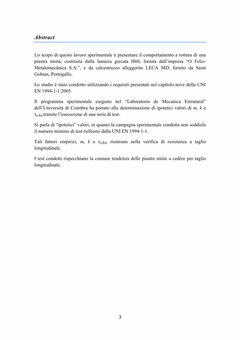
Lo scopo di questo lavoro sperimentale è presentare il comportamento a rottura di una piastra mista, costituita dalla lamiera grecata H60, fornita dall’impresa “O Feliz-Metalomecânica S.A.”, e da calcestruzzo alleggerito LECA MD, fornito da Saint Gobain, Portogallo.

Lo studio è stato condotto utilizzando i requisiti presentati nel capitolo nove della UNI EN 1994-1-1:2005.

Il programma sperimentale eseguito nel “Laboratorio de Mecanica Estrutural” dell’Università di Coimbra ha portato alla determinazione di ipotetici valori di m, k e τu,Rd tramite l’esecuzione di una serie di test.

Si parla di “ipotetici” valori, in quanto la campagna sperimentale condotta non soddisfa il numero minimo di test richiesto dalla UNI EN 1994-1-1.

Tali fattori empirici, m, k e τu,Rd, rientrano nella verifica di resistenza a taglio longitudinale.

I test condotti rispecchiano la comune tendenza delle piastre miste a cedere per taglio longitudinale.

4

Abstract

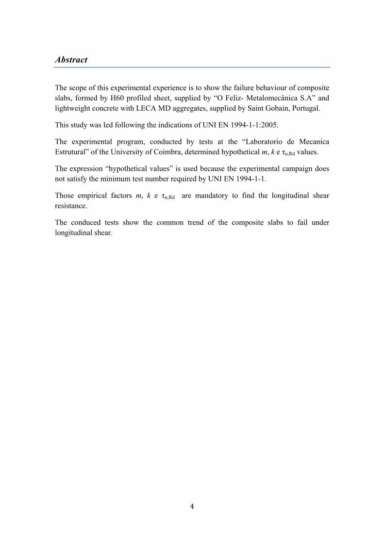
The scope of this experimental experience is to show the failure behaviour of composite slabs, formed by H60 profiled sheet, supplied by “O Feliz- Metalomecânica S.A” and lightweight concrete with LECA MD aggregates, supplied by Saint Gobain, Portugal.

This study was led following the indications of UNI EN 1994-1-1:2005.

The experimental program, conducted by tests at the “Laboratorio de Mecanica Estrutural” of the University of Coimbra, determined hypothetical m, k e τu,Rd values.

The expression “hypothetical values” is used because the experimental campaign does not satisfy the minimum test number required by UNI EN 1994-1-1.

Those empirical factors m, k e τu,Rd are mandatory to find the longitudinal shear resistance.

The conduced tests show the common trend of the composite slabs to fail under longitudinal shear.

5

Symbols Latin upper case letters A Cross-sectional area of the effective composite section neglecting concrete in

tension Ac Cross-sectional area of concrete A’p Cross-sectional area of profiled steel sheeting per unit width Ap Cross-sectional area of profiled steel sheeting Ape Effective cross-sectional area of profiled steel sheeting As Cross-sectional area of reinforcement As,x Cross-sectional area of reinforcement in x-axis As,y Cross-sectional area of reinforcement in y-axis Ecm Secant modulus of elasticity of concrete Es Modulus of elasticity of structural steel F Applied force Ic Second moment of area of the un-cracked concrete section, L Length; span; effective span Le Equivalent span Lo Length of overhang Lp Distance from centre of a concentrated load to the nearest support Ls Shear span Lx Distance from a cross-section to the nearest support LDC Low density concrete LWAC Lightweight aggregate concrete LWA Lightweight aggregate LWC Lightweight concrete M Bending moment MEd Design bending moment Mpa Design value of the plastic resistance moment of the effective cross-section of the

profiled steel sheeting Mpl,Rd Design value of the plastic resistance moment of the composite section with full

shear connection Mpr Reduced plastic resistance moment of the profiled steel sheeting MRd Design value of the resistance moment of a composite section or joint Mtest Test moment value N Compressive normal force; Nc Design value of the compressive normal force in the concrete flange Nc,f Design value of the compressive normal force in the concrete flange with full

shear connection NC Normal concrete Va,Ed Design value of the shear force acting on the structural steel section Vb,Rd Design value of the shear buckling resistance of a steel web VEd Design value of the shear force acting on the composite section Vl,Rd Design value of the resistance to shear Vpl,Rd Design value of the plastic resistance of the composite section to vertical shear

6

Vpl,a,Rd Design value of the plastic resistance of the structural steel section to vertical shear

Vp,Rd Design value of the resistance of a composite slab to punching shear VRd Design value of the resistance of the composite section to vertical shear Vt Support reaction Vv,Rd Design value of the resistance of a composite slab to vertical shear Wt Measured failure load Latin lower case letters b Width of the flange of a steel section; width of slab bem Effective width of a composite slab bm Width of a composite slab over which a load is distributed bp Length of concentrated line load br Width of rib of profiled steel sheeting bs Distance between centres of adjacent ribs of profiled steel sheeting b0 Distance between the centres of the outstand shear connectors; mean width of a

concrete rib (minimum width for re-entrant sheeting profiles) dp Distance between the centroidal axis of the profiled steel sheeting and the

extreme fibre of the composite slab in compression ds Distance between the steel reinforcement in tension to the extreme fibre of the

composite slab in compression e Distance from the centroidal axis of profiled steel sheeting to the extreme fibre

of the composite slab in tension ep Distance from the plastic neutral axis of profiled steel sheeting to the extreme

fibre of the composite slab in tension es Distance from the steel reinforcement in tension to the extreme fibre of the

composite slab in tension fcd Design value of the cylinder compressive strength of concrete fck Characteristic value of the cylinder compressive strength of concrete at 28 days fcm Mean value of the measured cylinder compressive strength of concrete fctm Mean value of the axial tensile strength of concrete flctm Mean value of the axial tensile strength of lightweight concrete fsd Design value of the yield strength of reinforcing steel fsk Characteristic value of the yield strength of reinforcing steel fu Specified ultimate tensile strength fy Nominal value of the yield strength of structural steel fyd Design value of the yield strength of structural steel fyp,d Design value of the yield strength of profiled steel sheeting fypm Mean value of the measured yield strength of profiled steel sheeting h Overall depth; thickness hc Thickness of concrete above the main flat surface of the top of the ribs of the

sheeting hp Overall depth of the profiled steel sheeting excluding embossments hs Distance between the longitudinal reinforcement in tension and the centre of

compression ht Overall thickness of test specimen k Empirical factor for design shear resistance

7

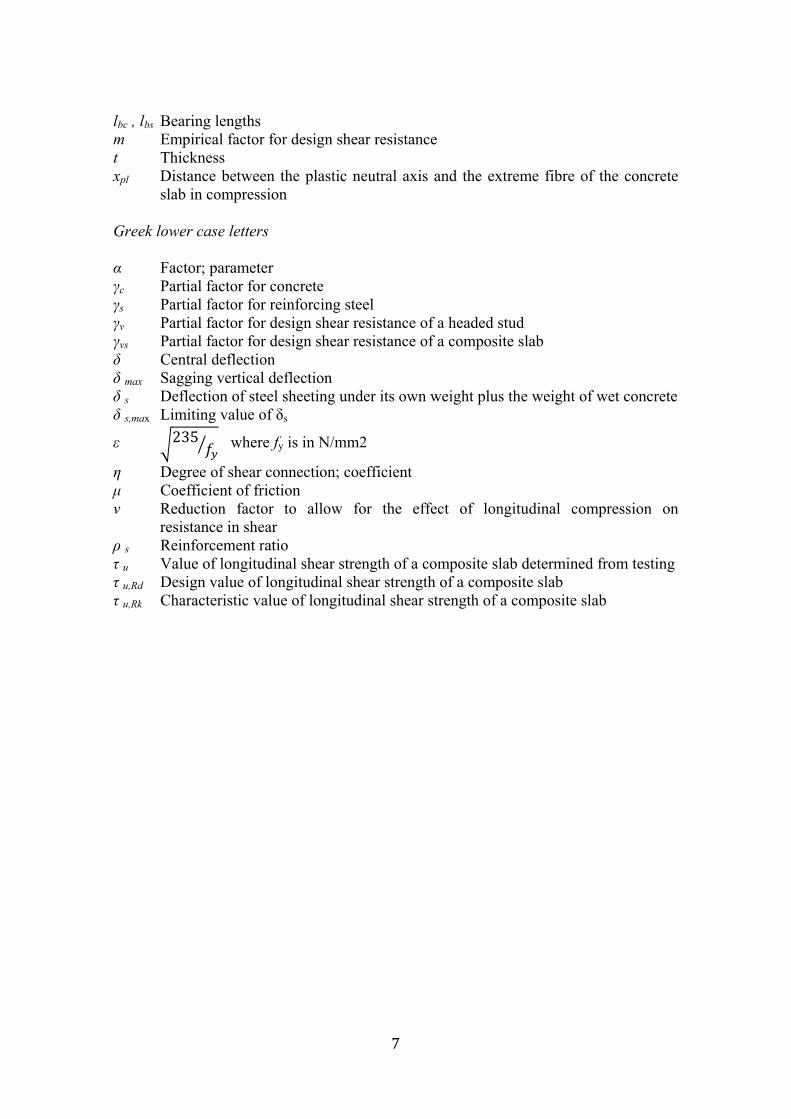
lbc , lbs Bearing lengths m Empirical factor for design shear resistance t Thickness xpl Distance between the plastic neutral axis and the extreme fibre of the concrete

slab in compression Greek lower case letters α Factor; parameter γc Partial factor for concrete γs Partial factor for reinforcing steel γv Partial factor for design shear resistance of a headed stud γvs Partial factor for design shear resistance of a composite slab δ Central deflection δ max Sagging vertical deflection δ s Deflection of steel sheeting under its own weight plus the weight of wet concrete δ s,max Limiting value of δs

ε �235𝑓𝑦� where fy is in N/mm2

η Degree of shear connection; coefficient μ Coefficient of friction ν Reduction factor to allow for the effect of longitudinal compression on

resistance in shear ρ s Reinforcement ratio τ u Value of longitudinal shear strength of a composite slab determined from testing τ u,Rd Design value of longitudinal shear strength of a composite slab τ u,Rk Characteristic value of longitudinal shear strength of a composite slab

8

Introduction

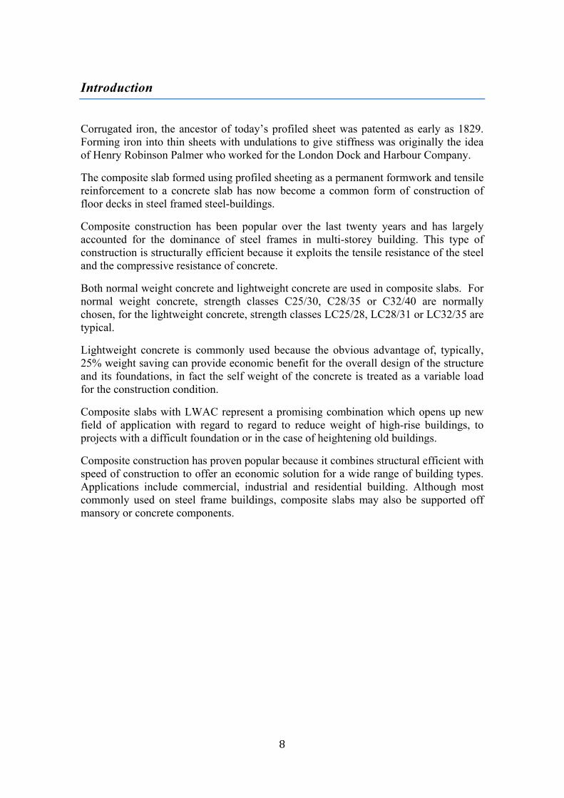
Corrugated iron, the ancestor of today’s profiled sheet was patented as early as 1829. Forming iron into thin sheets with undulations to give stiffness was originally the idea of Henry Robinson Palmer who worked for the London Dock and Harbour Company.

The composite slab formed using profiled sheeting as a permanent formwork and tensile reinforcement to a concrete slab has now become a common form of construction of floor decks in steel framed steel-buildings.

Composite construction has been popular over the last twenty years and has largely accounted for the dominance of steel frames in multi-storey building. This type of construction is structurally efficient because it exploits the tensile resistance of the steel and the compressive resistance of concrete.

Both normal weight concrete and lightweight concrete are used in composite slabs. For normal weight concrete, strength classes C25/30, C28/35 or C32/40 are normally chosen, for the lightweight concrete, strength classes LC25/28, LC28/31 or LC32/35 are typical.

Lightweight concrete is commonly used because the obvious advantage of, typically, 25% weight saving can provide economic benefit for the overall design of the structure and its foundations, in fact the self weight of the concrete is treated as a variable load for the construction condition.

Composite slabs with LWAC represent a promising combination which opens up new field of application with regard to regard to reduce weight of high-rise buildings, to projects with a difficult foundation or in the case of heightening old buildings.

Composite construction has proven popular because it combines structural efficient with speed of construction to offer an economic solution for a wide range of building types. Applications include commercial, industrial and residential building. Although most commonly used on steel frame buildings, composite slabs may also be supported off mansory or concrete components.

9

Composite Slabs

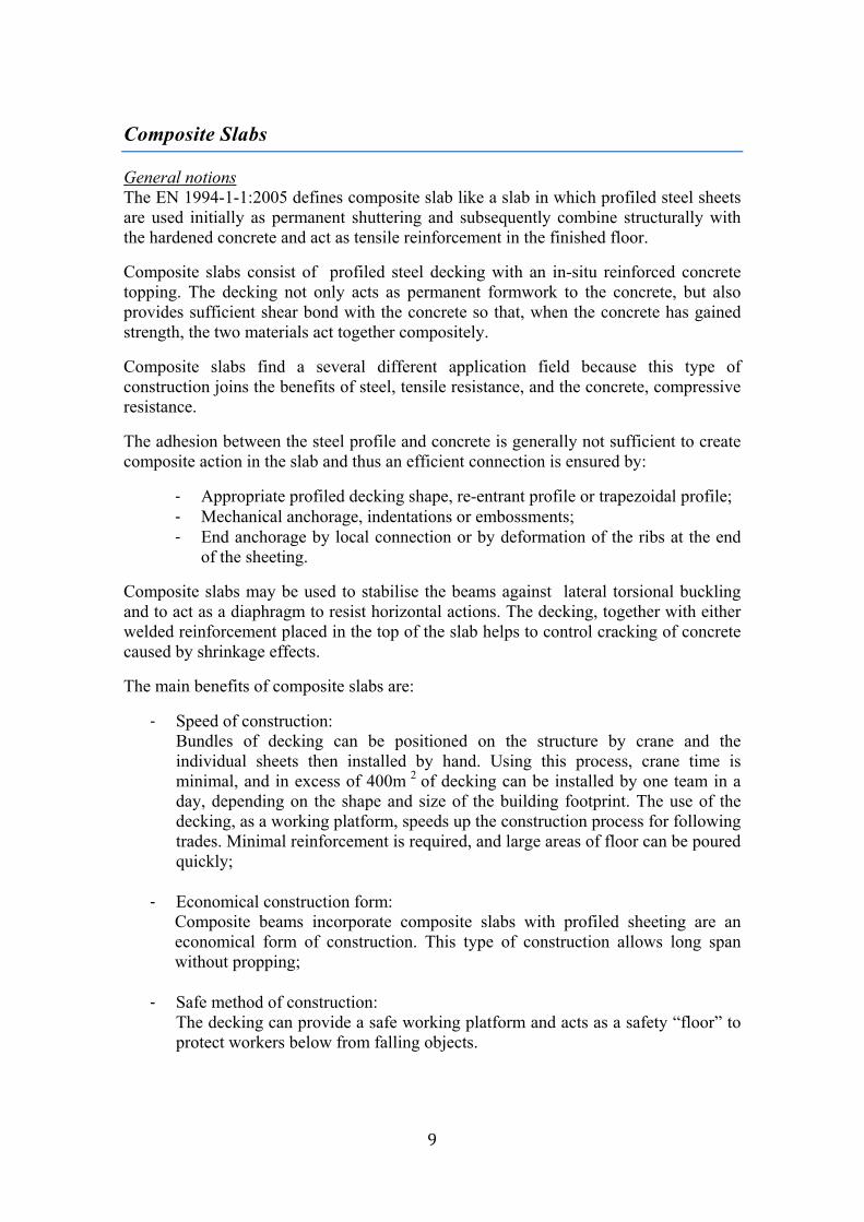
General notions The EN 1994-1-1:2005 defines composite slab like a slab in which profiled steel sheets are used initially as permanent shuttering and subsequently combine structurally with the hardened concrete and act as tensile reinforcement in the finished floor.

Composite slabs consist of profiled steel decking with an in-situ reinforced concrete topping. The decking not only acts as permanent formwork to the concrete, but also provides sufficient shear bond with the concrete so that, when the concrete has gained strength, the two materials act together compositely.

Composite slabs find a several different application field because this type of construction joins the benefits of steel, tensile resistance, and the concrete, compressive resistance.

The adhesion between the steel profile and concrete is generally not sufficient to create composite action in the slab and thus an efficient connection is ensured by:

- Appropriate profiled decking shape, re-entrant profile or trapezoidal profile; - Mechanical anchorage, indentations or embossments; - End anchorage by local connection or by deformation of the ribs at the end

of the sheeting.

Composite slabs may be used to stabilise the beams against lateral torsional buckling and to act as a diaphragm to resist horizontal actions. The decking, together with either welded reinforcement placed in the top of the slab helps to control cracking of concrete caused by shrinkage effects.

The main benefits of composite slabs are:

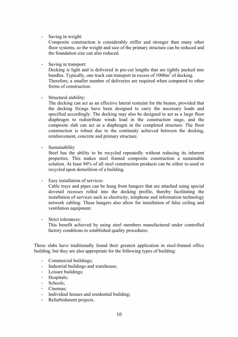
- Speed of construction: Bundles of decking can be positioned on the structure by crane and the individual sheets then installed by hand. Using this process, crane time is minimal, and in excess of 400m 2 of decking can be installed by one team in a day, depending on the shape and size of the building footprint. The use of the decking, as a working platform, speeds up the construction process for following trades. Minimal reinforcement is required, and large areas of floor can be poured quickly;

- Economical construction form: Composite beams incorporate composite slabs with profiled sheeting are an economical form of construction. This type of construction allows long span without propping;

- Safe method of construction:

The decking can provide a safe working platform and acts as a safety “floor” to protect workers below from falling objects.

10

- Saving in weight: Composite construction is considerably stiffer and stronger than many other floor systems, so the weight and size of the primary structure can be reduced and the foundation size can also reduced.

- Saving in transport: Decking is light and is delivered in pre-cut lengths that are tightly packed into bundles. Typically, one truck can transport in excess of 1000m2 of decking. Therefore, a smaller number of deliveries are required when compared to other forms of construction.

- Structural stability: The decking can act as an effective lateral restraint for the beams, provided that the decking fixings have been designed to carry the necessary loads and specified accordingly. The decking may also be designed to act as a large floor diaphragm to redistribute winds load in the construction stage, and the composite slab can act as a diaphragm in the completed structure. The floor construction is robust due to the continuity achieved between the decking, reinforcement, concrete and primary structure.

- Sustainability Steel has the ability to be recycled repeatedly without reducing its inherent properties. This makes steel framed composite construction a sustainable solution. At least 94% of all steel construction products can be either re-used or recycled upon demolition of a building.

- Easy installation of services: Cable trays and pipes can be hung from hangers that are attached using special dovetail recesses rolled into the decking profile, thereby facilitating the installation of services such as electricity, telephone and information technology network cabling. These hangers also allow for installation of false ceiling and ventilation equipment.

- Strict tolerances:

This benefit achieved by using steel members manufactured under controlled factory conditions to established quality procedures.

These slabs have traditionally found their greatest application in steel-framed office building, but they are also appropriate for the following types of building:

- Commercial buildings; - Industrial buildings and warehouse; - Leisure buildings; - Hospitals; - Schools; - Cinemas; - Individual houses and residential building; - Refurbishment projects.

11

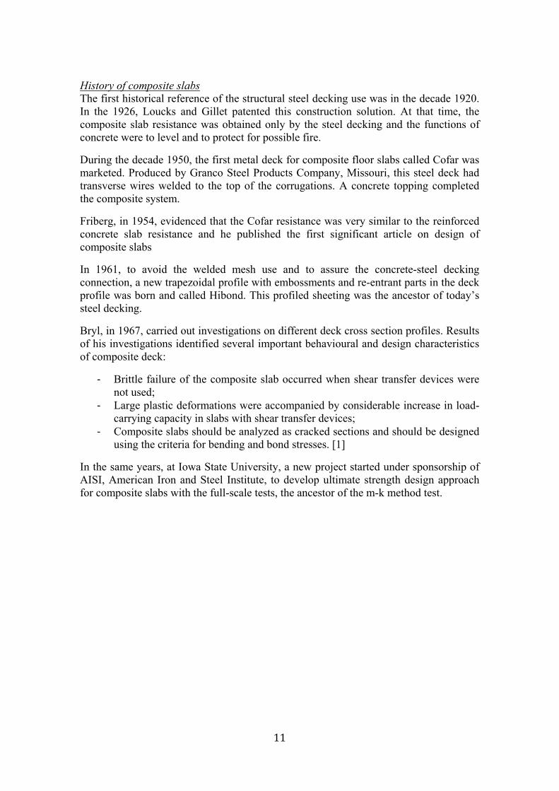
History of composite slabs The first historical reference of the structural steel decking use was in the decade 1920. In the 1926, Loucks and Gillet patented this construction solution. At that time, the composite slab resistance was obtained only by the steel decking and the functions of concrete were to level and to protect for possible fire.

During the decade 1950, the first metal deck for composite floor slabs called Cofar was marketed. Produced by Granco Steel Products Company, Missouri, this steel deck had transverse wires welded to the top of the corrugations. A concrete topping completed the composite system.

Friberg, in 1954, evidenced that the Cofar resistance was very similar to the reinforced concrete slab resistance and he published the first significant article on design of composite slabs

In 1961, to avoid the welded mesh use and to assure the concrete-steel decking connection, a new trapezoidal profile with embossments and re-entrant parts in the deck profile was born and called Hibond. This profiled sheeting was the ancestor of today’s steel decking.

Bryl, in 1967, carried out investigations on different deck cross section profiles. Results of his investigations identified several important behavioural and design characteristics of composite deck:

- Brittle failure of the composite slab occurred when shear transfer devices were not used;

- Large plastic deformations were accompanied by considerable increase in load-carrying capacity in slabs with shear transfer devices;

- Composite slabs should be analyzed as cracked sections and should be designed using the criteria for bending and bond stresses. [1]

In the same years, at Iowa State University, a new project started under sponsorship of AISI, American Iron and Steel Institute, to develop ultimate strength design approach for composite slabs with the full-scale tests, the ancestor of the m-k method test.

12

Steel decking

General Notions Numerous types of profiled decking are used in composite slabs. The different sheeting types present different shapes, depth and distance between ribs, width, lateral covering, plane stiffeners and mechanical connections between steel sheeting and concrete. The profiled sheeting characteristics are generally the following:

- Thickness between 0,75mm and 1,5mm and in most cases between 0,75mm and 1mm; the recommended values in the National Annex of EN 1994-1-1 is t ≥ 0,70mm;

- Standard protection against corrosion by a thin layer of galvanizing on both

faces for durability purpose: peculiar care should be taken on the thickness that is used in design owing to the fact that the sheet thickness that is often quoted by manufacturers in the overall thickness, including the galvanized coating. The steel is galvanized before forming, and this is designated in the steel grade by the letter GD, followed by a number corresponding to the number of grams of zinc per m2.

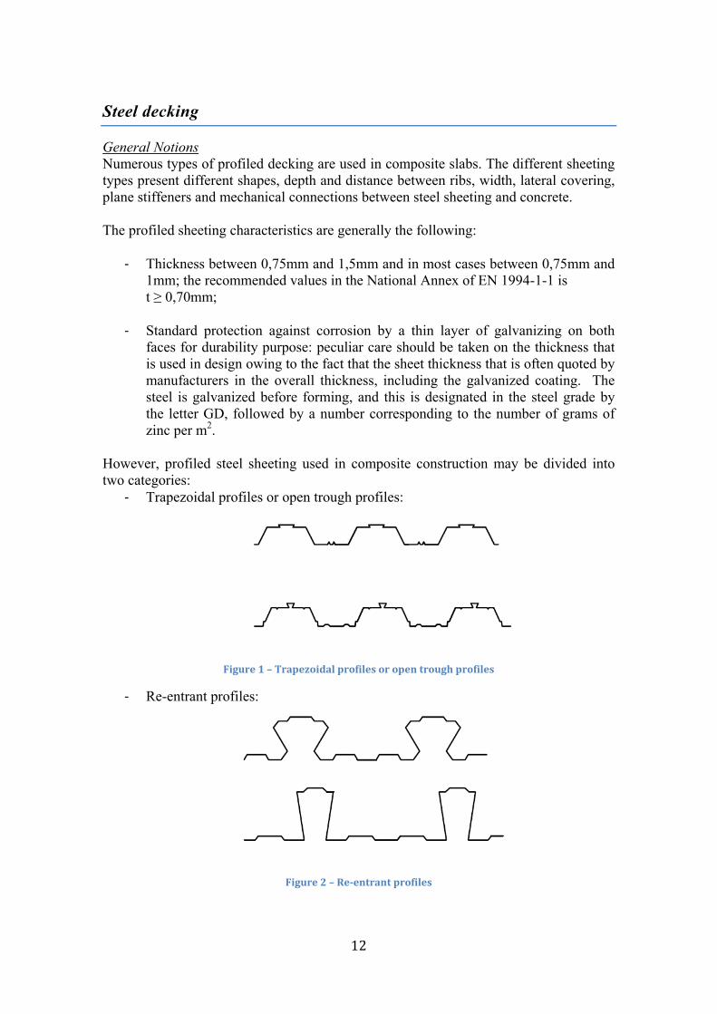
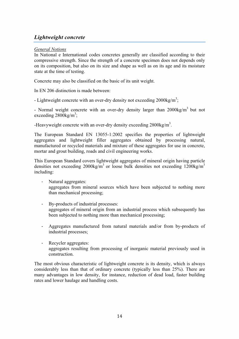
However, profiled steel sheeting used in composite construction may be divided into two categories:

- Trapezoidal profiles or open trough profiles:

Figure 1 – Trapezoidal profiles or open trough profiles

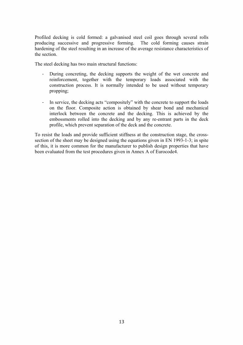
- Re-entrant profiles:

Figure 2 – Re-entrant profiles

13

Profiled decking is cold formed: a galvanised steel coil goes through several rolls producing successive and progressive forming. The cold forming causes strain hardening of the steel resulting in an increase of the average resistance characteristics of the section.

The steel decking has two main structural functions:

- During concreting, the decking supports the weight of the wet concrete and reinforcement, together with the temporary loads associated with the construction process. It is normally intended to be used without temporary propping;

- In service, the decking acts “compositely” with the concrete to support the loads on the floor. Composite action is obtained by shear bond and mechanical interlock between the concrete and the decking. This is achieved by the embossments rolled into the decking and by any re-entrant parts in the deck profile, which prevent separation of the deck and the concrete.

To resist the loads and provide sufficient stiffness at the construction stage, the cross-section of the sheet may be designed using the equations given in EN 1993-1-3; in spite of this, it is more common for the manufacturer to publish design properties that have been evaluated from the test procedures given in Annex A of Eurocode4.

14

Lightweight concrete

General Notions In National e International codes concretes generally are classified according to their compressive strength. Since the strength of a concrete specimen does not depends only on its composition, but also on its size and shape as well as on its age and its moisture state at the time of testing.

Concrete may also be classified on the basic of its unit weight.

In EN 206 distinction is made between:

- Lightweight concrete with an over-dry density not exceeding 2000kg/m3;

- Normal weight concrete with an over-dry density larger than 2000kg/m3 but not exceeding 2800kg/m3;

-Heavyweight concrete with an over-dry density exceeding 2800kg/m3.

The European Standard EN 13055-1:2002 specifies the properties of lightweight aggregates and lightweight filler aggregates obtained by processing natural, manufactured or recycled materials and mixture of these aggregates for use in concrete, mortar and grout building, roads and civil engineering works.

This European Standard covers lightweight aggregates of mineral origin having particle densities not exceeding 2000kg/m3 or loose bulk densities not exceeding 1200kg/m3 including:

- Natural aggregates: aggregates from mineral sources which have been subjected to nothing more than mechanical processing;

- By-products of industrial processes: aggregates of mineral origin from an industrial process which subsequently has been subjected to nothing more than mechanical processing;

- Aggregates manufactured from natural materials and/or from by-products of industrial processes;

- Recycler aggregates: aggregates resulting from processing of inorganic material previously used in construction.

The most obvious characteristic of lightweight concrete is its density, which is always considerably less than that of ordinary concrete (typically less than 25%). There are many advantages in low density, for instance, reduction of dead load, faster building rates and lower haulage and handling costs.

15

The economy of LWAC (lightweight aggregate concrete) relies on a large extent on the possible reduction of weight. The strength of the aggregates appears, in particular when the weight is reduced to a minimum, to be the decisive factor for the LWAC. The challenges for the aggregate industry are thus to produce an aggregate with:

-High strength;

-Low weight;

-Good production properties, low water absorption;

-Reasonable price.

Industries has demonstrated under laboratory conditions the possibilities to produce LWA satisfying the first three requirement, but for the last requirement there is still a lot of problem.

Another characteristic of LWAC has been showed experimentally and by practical experience in the industry that faster building rates can be achieved with lightweight concrete than with the more traditional materials, and for this reason many builders today are prefer to pay considerably more for lightweight concrete units than for bricks, for the same area.

A less obvious but none the less important characteristic of lightweight concrete is the relatively low thermal conductivity that it possesses; this property improves with decreasing density.

Quite apart from their technical advantage in building, some lightweight concretes have the additional merit of providing an outlet for industrial wastes (clinker, pulverised fuel ash and blast-furnace slag).

Waste represented an ever-increasing problem in society. A promising possibility is to use waste materials as raw materials for manufactured aggregates. When the raw material has a negative price, the economy in the aggregates produced is very influenced. Sintered fly ash is an example of a manufactured aggregate of this type.

16

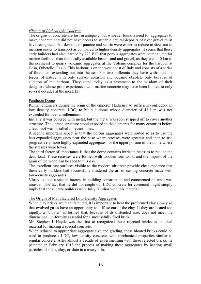
History of Lightweight Concrete The origins of concrete are lost in antiquity, but whoever found a need for aggregates to make concrete and did not have access to suitable natural deposits of river gravel must have recognized that deposits of pumice and scoria were easier to reduce to size, not to mention easier to transport as compared to higher density aggregates. It seems that these early builders had also learned by 273 B.C. that porous aggregates were better suited for marine facilities than the locally available beach sand and gravel, as they went 40 km to the northeast to quarry volcanic aggregates at the Volcine complex for the harbour at Cosa, Orbetello, Lazio. This harbour is on the west coast of Italy and consists of a series of four piers extending out into the sea. For two millennia they have withstood the forces of nature with only surface abrasion and became obsolete only because of siltation of the harbour. They stand today as a testament to the wisdom of their designers whose prior experiences with marine concrete may have been limited to only several decades at the most. [2] Pantheon Dome Roman engineers during the reign of the emperor Hadrian had sufficient confidence in low density concrete, LDC, to build a dome whose diameter of 43.3 m was not exceeded for over a millennium. Initially it was covered with metal, but the metal was soon stripped off to cover another structure. The domed structure stood exposed to the elements for many centuries before a lead roof was installed in recent times. A second important aspect is that the porous aggregates were sorted so as to use the less-expanded aggregates near the base where stresses were greatest and then to use progressively more highly expanded aggregates for the upper portion of the dome where the stresses were lower. The third factor of importance is that the dome contains intricate recesses to reduce the dead load. These recesses were formed with wooden formwork, and the imprint of the grain of the wood can be seen to this day. The excellent cast surfaces visible to the modern observer provide clear evidence that these early builders had successfully mastered the art of casting concrete made with low-density aggregates. Vitruvius took a special interest in building construction and commented on what was unusual. The fact that he did not single out LDC concrete for comment might simply imply that these early builders were fully familiar with this material. The Origin of Manufactured Low-Density Aggregates When clay bricks are manufactured, it is important to heat the preformed clay slowly so that evolved gases have an opportunity to diffuse out of the clay. If they are heated too rapidly, a “bloater” is formed that, because of its distended size, does not meet the dimensional uniformity essential for a successfully fired brick. Mr. Stephen J. Hayde was the first to recognized those rejected bricks as an ideal material for making a special concrete. When reduced to appropriate aggregate size and grading, these bloated bricks could be used to produce a LDC, low density concrete, with mechanical properties similar to regular concrete. After almost a decade of experimenting with these rejected bricks, he patented in February 1918 the process of making these aggregates by heating small particles of shale, clay, or slate in a rotary kiln.

17

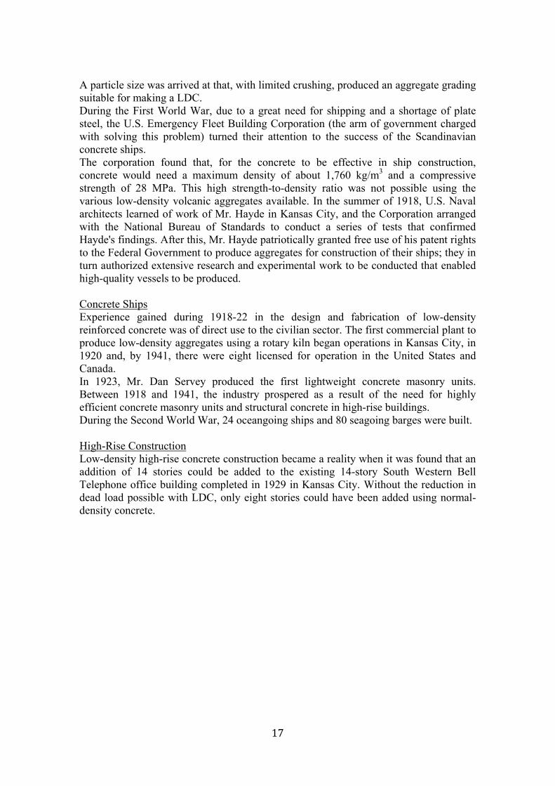
A particle size was arrived at that, with limited crushing, produced an aggregate grading suitable for making a LDC. During the First World War, due to a great need for shipping and a shortage of plate steel, the U.S. Emergency Fleet Building Corporation (the arm of government charged with solving this problem) turned their attention to the success of the Scandinavian concrete ships. The corporation found that, for the concrete to be effective in ship construction, concrete would need a maximum density of about 1,760 kg/m3 and a compressive strength of 28 MPa. This high strength-to-density ratio was not possible using the various low-density volcanic aggregates available. In the summer of 1918, U.S. Naval architects learned of work of Mr. Hayde in Kansas City, and the Corporation arranged with the National Bureau of Standards to conduct a series of tests that confirmed Hayde's findings. After this, Mr. Hayde patriotically granted free use of his patent rights to the Federal Government to produce aggregates for construction of their ships; they in turn authorized extensive research and experimental work to be conducted that enabled high-quality vessels to be produced. Concrete Ships Experience gained during 1918-22 in the design and fabrication of low-density reinforced concrete was of direct use to the civilian sector. The first commercial plant to produce low-density aggregates using a rotary kiln began operations in Kansas City, in 1920 and, by 1941, there were eight licensed for operation in the United States and Canada. In 1923, Mr. Dan Servey produced the first lightweight concrete masonry units. Between 1918 and 1941, the industry prospered as a result of the need for highly efficient concrete masonry units and structural concrete in high-rise buildings. During the Second World War, 24 oceangoing ships and 80 seagoing barges were built. High-Rise Construction Low-density high-rise concrete construction became a reality when it was found that an addition of 14 stories could be added to the existing 14-story South Western Bell Telephone office building completed in 1929 in Kansas City. Without the reduction in dead load possible with LDC, only eight stories could have been added using normal-density concrete.

18

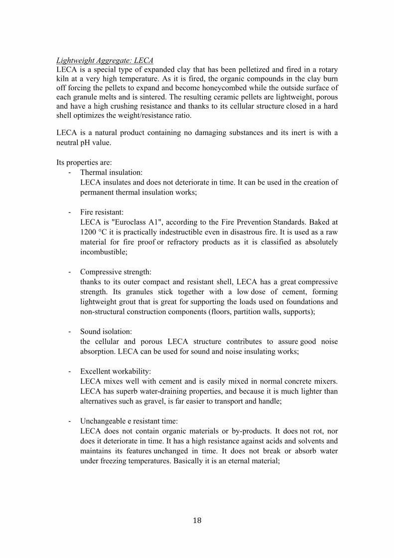
Lightweight Aggregate: LECA LECA is a special type of expanded clay that has been pelletized and fired in a rotary kiln at a very high temperature. As it is fired, the organic compounds in the clay burn off forcing the pellets to expand and become honeycombed while the outside surface of each granule melts and is sintered. The resulting ceramic pellets are lightweight, porous and have a high crushing resistance and thanks to its cellular structure closed in a hard shell optimizes the weight/resistance ratio.

LECA is a natural product containing no damaging substances and its inert is with a neutral pH value. Its properties are:

- Thermal insulation: LECA insulates and does not deteriorate in time. It can be used in the creation of permanent thermal insulation works;

- Fire resistant:

LECA is "Euroclass A1", according to the Fire Prevention Standards. Baked at 1200 °C it is practically indestructible even in disastrous fire. It is used as a raw material for fire proof or refractory products as it is classified as absolutely incombustible;

- Compressive strength: thanks to its outer compact and resistant shell, LECA has a great compressive strength. Its granules stick together with a low dose of cement, forming lightweight grout that is great for supporting the loads used on foundations and non-structural construction components (floors, partition walls, supports);

- Sound isolation: the cellular and porous LECA structure contributes to assure good noise absorption. LECA can be used for sound and noise insulating works;

- Excellent workability:

LECA mixes well with cement and is easily mixed in normal concrete mixers. LECA has superb water-draining properties, and because it is much lighter than alternatives such as gravel, is far easier to transport and handle;

- Unchangeable e resistant time: LECA does not contain organic materials or by-products. It does not rot, nor does it deteriorate in time. It has a high resistance against acids and solvents and maintains its features unchanged in time. It does not break or absorb water under freezing temperatures. Basically it is an eternal material;

19

- Natural e environment-friendly: LECA does not contain, nor releases silica, fibrous substances, radon gas or other harmful materials, not even in the event of fire. It is a natural and environment-friendly product.

Before to use, LECA specific humidity must know. In fact if the aggregate is dry, it is able to absorb part of the water of mixture. This means that the concrete needs more water and consequently the mix design and all of its performances change.

20

Experimental process: Lightweight concrete

The mix design study of LWC has been developed in the University of Minho, in Guimaraes, with the collaboration of the Prof. Isabel Valente.

The first step in the LWC study was the test for geometrical proprieties of aggregates. This part has been developed with the EN 933-1:2000 to determine the particle size distribution with the sieving method.

This part of the standard specifies nominal aperture sizes and shape for woven wire cloth and perforated plate in test sieves used for test methods for aggregates. It applies to aggregates of natural or artificial origin including lightweight aggregates.

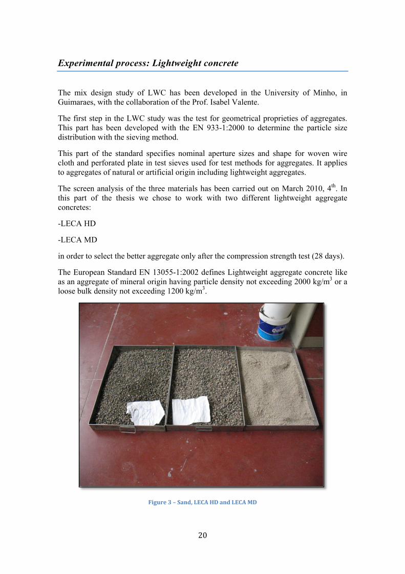
The screen analysis of the three materials has been carried out on March 2010, 4th. In this part of the thesis we chose to work with two different lightweight aggregate concretes:

-LECA HD

-LECA MD

in order to select the better aggregate only after the compression strength test (28 days).

The European Standard EN 13055-1:2002 defines Lightweight aggregate concrete like as an aggregate of mineral origin having particle density not exceeding 2000 kg/m3 or a loose bulk density not exceeding 1200 kg/m3.

Figure 3 – Sand, LECA HD and LECA MD

21

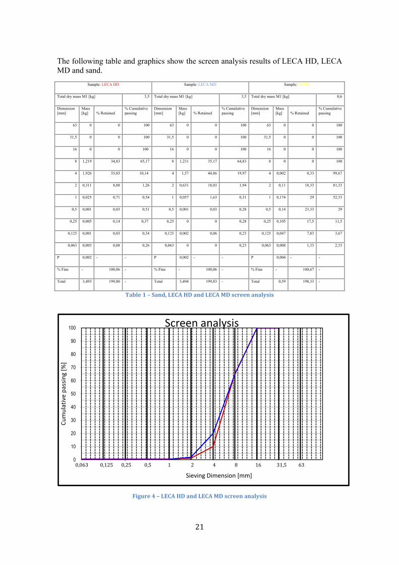
The following table and graphics show the screen analysis results of LECA HD, LECA MD and sand.

Sample: LECA HD Sample: LECA MD Sample: SAND

Total dry mass M1 [kg] 3,5 Total dry mass M1 [kg] 3,5 Total dry mass M1 [kg] 0,6

Dimension [mm]

Mass [kg] % Retained

% Cumulative passing

Dimension [mm]

Mass [kg] % Retained

% Cumulative passing

Dimension [mm]

Mass [kg] % Retained

% Cumulative passing

63 0 0 100 63 0 0 100 63 0 0 100

31,5 0 0 100 31,5 0 0 100 31,5 0 0 100

16 0 0 100 16 0 0 100 16 0 0 100

8 1,219 34,83 65,17 8 1,231 35,17 64,83 8 0 0 100

4 1,926 55,03 10,14 4 1,57 44,86 19,97 4 0,002 0,33 99,67

2 0,311 8,88 1,26 2 0,631 18,03 1,94 2 0,11 18,33 81,33

1 0,025 0,71 0,54 1 0,057 1,63 0,31 1 0,174 29 52,33

0,5 0,001 0,03 0,51 0,5 0,001 0,03 0,28 0,5 0,14 23,33 29

0,25 0,005 0,14 0,37 0,25 0 0 0,28 0,25 0,105 17,5 11,5

0,125 0,001 0,03 0,34 0,125 0,002 0,06 0,23 0,125 0,047 7,83 3,67

0,063 0,003 0,08 0,26 0,063 0 0 0,23 0,063 0,008 1,33 2,33

P 0,002 - - P 0,002 - - P 0,004 - -

% Fine - 100,06 - % Fine - 100,06 - % Fine - 100,67 -

Total 3,493 199,80 - Total 3,494 199,83 - Total 0,59 198,33 -

Table 1 – Sand, LECA HD and LECA MD screen analysis

Figure 4 – LECA HD and LECA MD screen analysis

0

10

20

30

40

50

60

70

80

90

100

Cum

ulat

ive

pass

ing

[%]

Sieving Dimension [mm]

Screen analysis

0,063 0,125 0,25 0,5 1 2 4 8 16 31,5 63

22

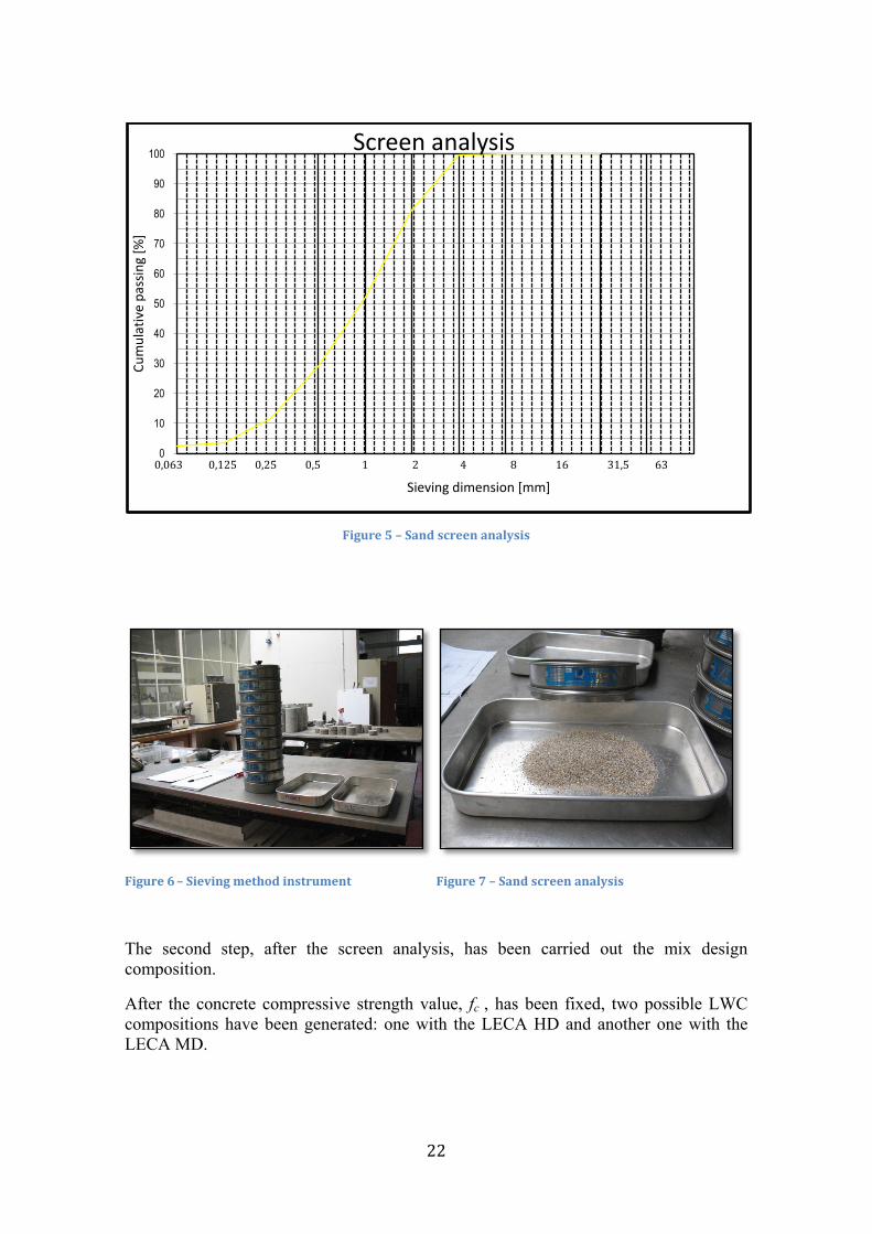
Figure 5 – Sand screen analysis

Figure 6 – Sieving method instrument Figure 7 – Sand screen analysis

The second step, after the screen analysis, has been carried out the mix design composition.

After the concrete compressive strength value, fc , has been fixed, two possible LWC compositions have been generated: one with the LECA HD and another one with the LECA MD.

0

10

20

30

40

50

60

70

80

90

100Cu

mul

ativ

e pa

ssin

g [%

]

Sieving dimension [mm]

Screen analysis

0,063 0,125 0,25 0,5 1 2 4 8 16 31,5 63

23

The following table shows mix design with LECA HD and LECA MD only for 50l of concrete, 0,05m2, equivalent to 6 cylindrical moulds and 4 cubic moulds.

LECA HD LECA MD Sand [kg] 32.8 30.8 LECA [kg] 20.5 15 Cement [kg] 20 20 Water [l] 5.622 5.622 Superplasticizer [l] 0.25 0.25

Table 2 - Mix design

The low amount of LECA MD in the mix design permitted to pond only 6 cylindrical moulds and 2 cubic moulds.

The concrete mixing has been prepared on March 5th, and in the same day we estimated the concrete drop below the mould; this represents the slump.

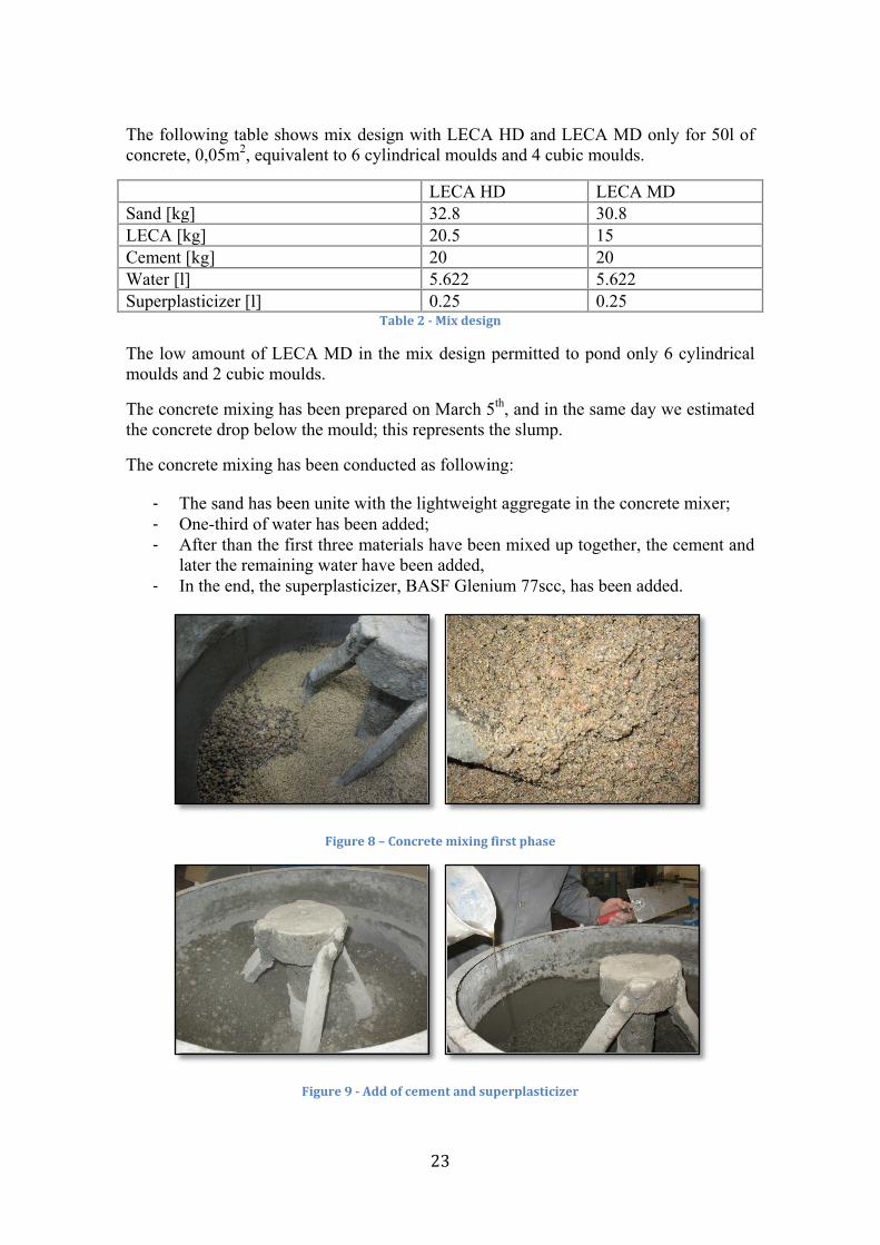
The concrete mixing has been conducted as following:

- The sand has been unite with the lightweight aggregate in the concrete mixer; - One-third of water has been added; - After than the first three materials have been mixed up together, the cement and

later the remaining water have been added, - In the end, the superplasticizer, BASF Glenium 77scc, has been added.

Figure 8 – Concrete mixing first phase

Figure 9 - Add of cement and superplasticizer

24

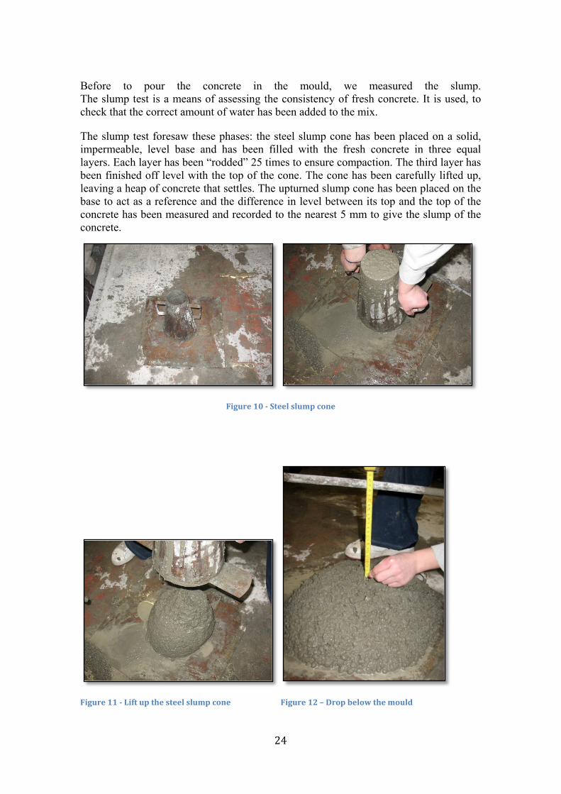
Before to pour the concrete in the mould, we measured the slump. The slump test is a means of assessing the consistency of fresh concrete. It is used, to check that the correct amount of water has been added to the mix.

The slump test foresaw these phases: the steel slump cone has been placed on a solid, impermeable, level base and has been filled with the fresh concrete in three equal layers. Each layer has been “rodded” 25 times to ensure compaction. The third layer has been finished off level with the top of the cone. The cone has been carefully lifted up, leaving a heap of concrete that settles. The upturned slump cone has been placed on the base to act as a reference and the difference in level between its top and the top of the concrete has been measured and recorded to the nearest 5 mm to give the slump of the concrete.

Figure 10 - Steel slump cone

Figure 11 - Lift up the steel slump cone Figure 12 – Drop below the mould

25

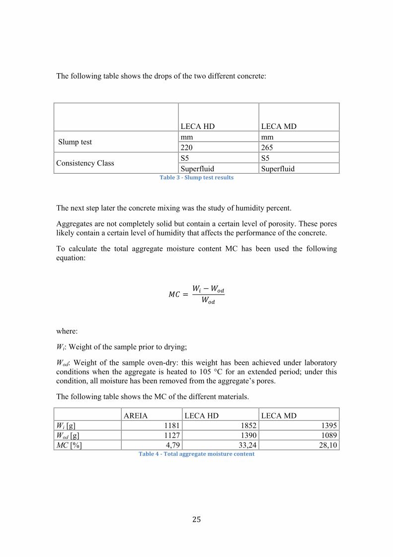
The following table shows the drops of the two different concrete:

LECA HD LECA MD

Slump test mm mm 220 265

Consistency Class S5 S5 Superfluid Superfluid

Table 3 - Slump test results

The next step later the concrete mixing was the study of humidity percent.

Aggregates are not completely solid but contain a certain level of porosity. These pores likely contain a certain level of humidity that affects the performance of the concrete.

To calculate the total aggregate moisture content MC has been used the following equation:

𝑀𝐶 = 𝑊𝑖 −𝑊𝑜𝑑

𝑊𝑜𝑑

where:

Wi: Weight of the sample prior to drying;

Wod: Weight of the sample oven-dry: this weight has been achieved under laboratory conditions when the aggregate is heated to 105 °C for an extended period; under this condition, all moisture has been removed from the aggregate’s pores.

The following table shows the MC of the different materials.

AREIA LECA HD LECA MD Wi [g] 1181 1852 1395 Wod [g] 1127 1390 1089 MC [%] 4,79 33,24 28,10

Table 4 - Total aggregate moisture content

26

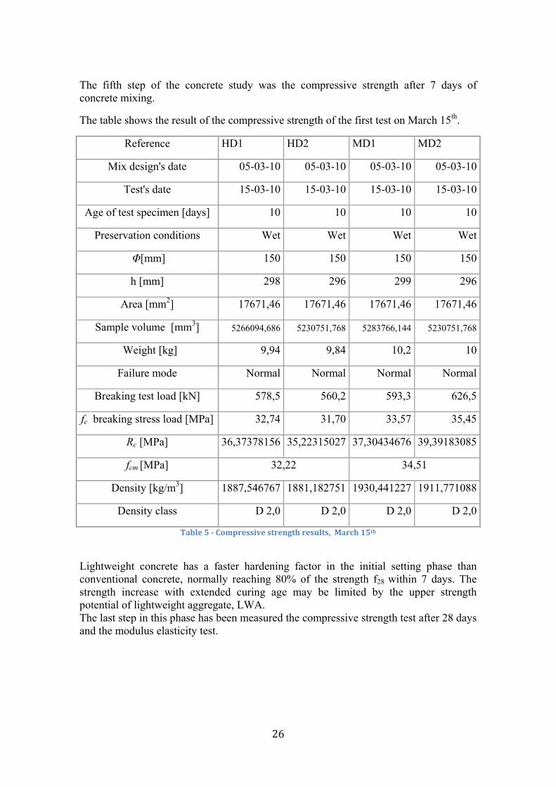
The fifth step of the concrete study was the compressive strength after 7 days of concrete mixing.

The table shows the result of the compressive strength of the first test on March 15th.

Reference HD1 HD2 MD1 MD2

Mix design's date 05-03-10 05-03-10 05-03-10 05-03-10

Test's date 15-03-10 15-03-10 15-03-10 15-03-10

Age of test specimen [days] 10 10 10 10

Preservation conditions Wet Wet Wet Wet

Φ[mm] 150 150 150 150

h [mm] 298 296 299 296

Area [mm2] 17671,46 17671,46 17671,46 17671,46

Sample volume [mm3] 5266094,686 5230751,768 5283766,144 5230751,768

Weight [kg] 9,94 9,84 10,2 10

Failure mode Normal Normal Normal Normal

Breaking test load [kN] 578,5 560,2 593,3 626,5

fc breaking stress load [MPa] 32,74 31,70 33,57 35,45

Rc [MPa] 36,37378156 35,22315027 37,30434676 39,39183085

fcm [MPa] 32,22 34,51

Density [kg/m3] 1887,546767 1881,182751 1930,441227 1911,771088

Density class D 2,0 D 2,0 D 2,0 D 2,0

Table 5 - Compressive strength results, March 15th

Lightweight concrete has a faster hardening factor in the initial setting phase than conventional concrete, normally reaching 80% of the strength f28 within 7 days. The strength increase with extended curing age may be limited by the upper strength potential of lightweight aggregate, LWA. The last step in this phase has been measured the compressive strength test after 28 days and the modulus elasticity test.

27

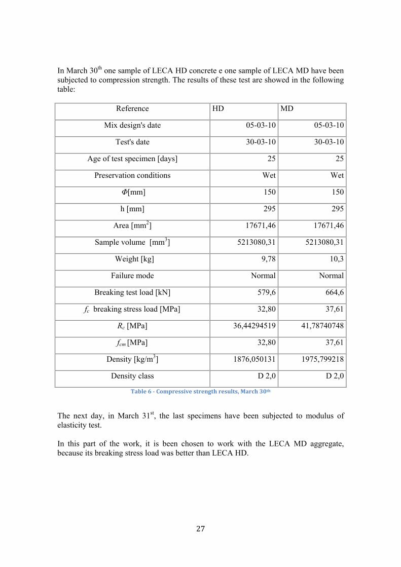
In March 30th one sample of LECA HD concrete e one sample of LECA MD have been subjected to compression strength. The results of these test are showed in the following table:

Reference HD MD

Mix design's date 05-03-10 05-03-10

Test's date 30-03-10 30-03-10

Age of test specimen [days] 25 25

Preservation conditions Wet Wet

Φ[mm] 150 150

h [mm] 295 295

Area [mm2] 17671,46 17671,46

Sample volume [mm3] 5213080,31 5213080,31

Weight [kg] 9,78 10,3

Failure mode Normal Normal

Breaking test load [kN] 579,6 664,6

fc breaking stress load [MPa] 32,80 37,61

Rc [MPa] 36,44294519 41,78740748

fcm [MPa] 32,80 37,61

Density [kg/m3] 1876,050131 1975,799218

Density class D 2,0 D 2,0

Table 6 - Compressive strength results, March 30th

The next day, in March 31st, the last specimens have been subjected to modulus of elasticity test. In this part of the work, it is been chosen to work with the LECA MD aggregate, because its breaking stress load was better than LECA HD.

28

The modulus of elasticity is defined as the ratio between the stress and the reversible strain. The section 3.1.3 of UNI EN 1992-1-1:2005 says that the modulus of elasticity of a concrete is controlled by the modulus of elasticity of its components. An estimate mean values of the secant modulus Elcm for LWC may be obtained by multiplying the values shows in the Table 3.1 of EN 1992-1-1, for normal density concrete, by the following coefficient:

𝜂𝐸 = (𝜌 − 2200)2 where ρ denotes the oven-dry density in accordance with EN 206-1 Section 4:

Density class 1 1,2 1,4 1,6 1,8 2

Density [kg/m3] 801 1001 1201 1401 1601 1801 1000 1200 1400 1600 1800 2000

Table 7 - Density class

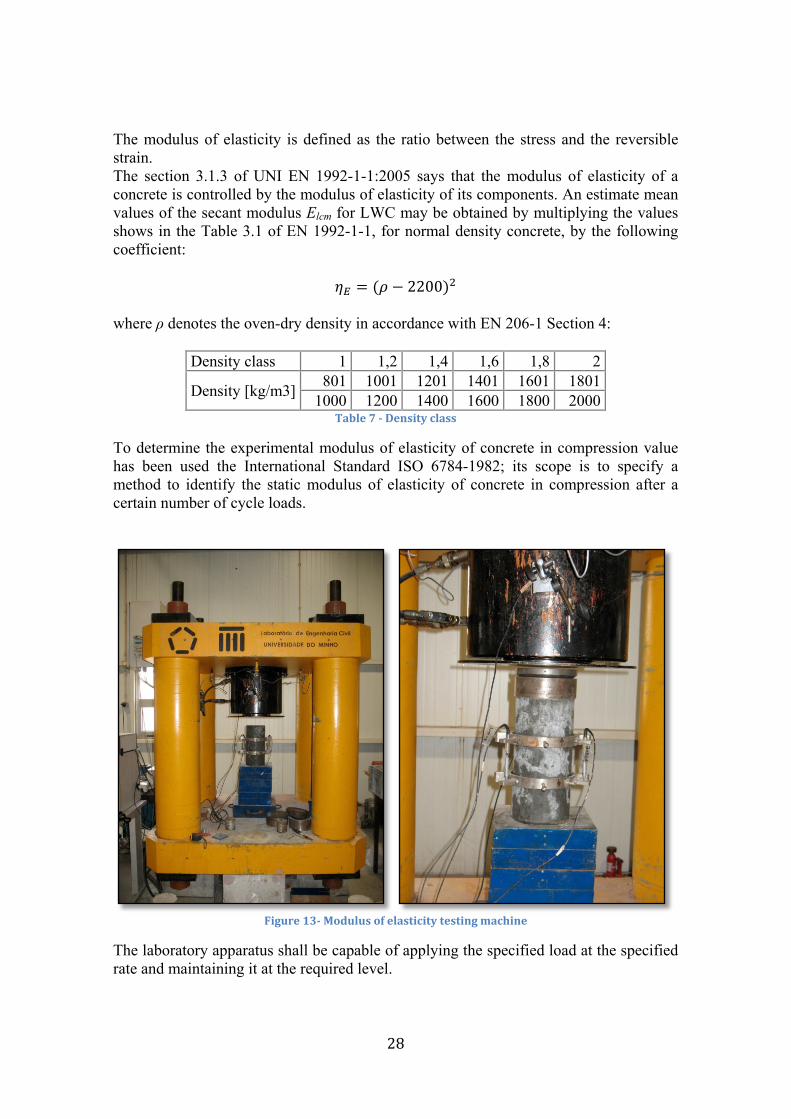
To determine the experimental modulus of elasticity of concrete in compression value has been used the International Standard ISO 6784-1982; its scope is to specify a method to identify the static modulus of elasticity of concrete in compression after a certain number of cycle loads.

Figure 13- Modulus of elasticity testing machine

The laboratory apparatus shall be capable of applying the specified load at the specified rate and maintaining it at the required level.

29

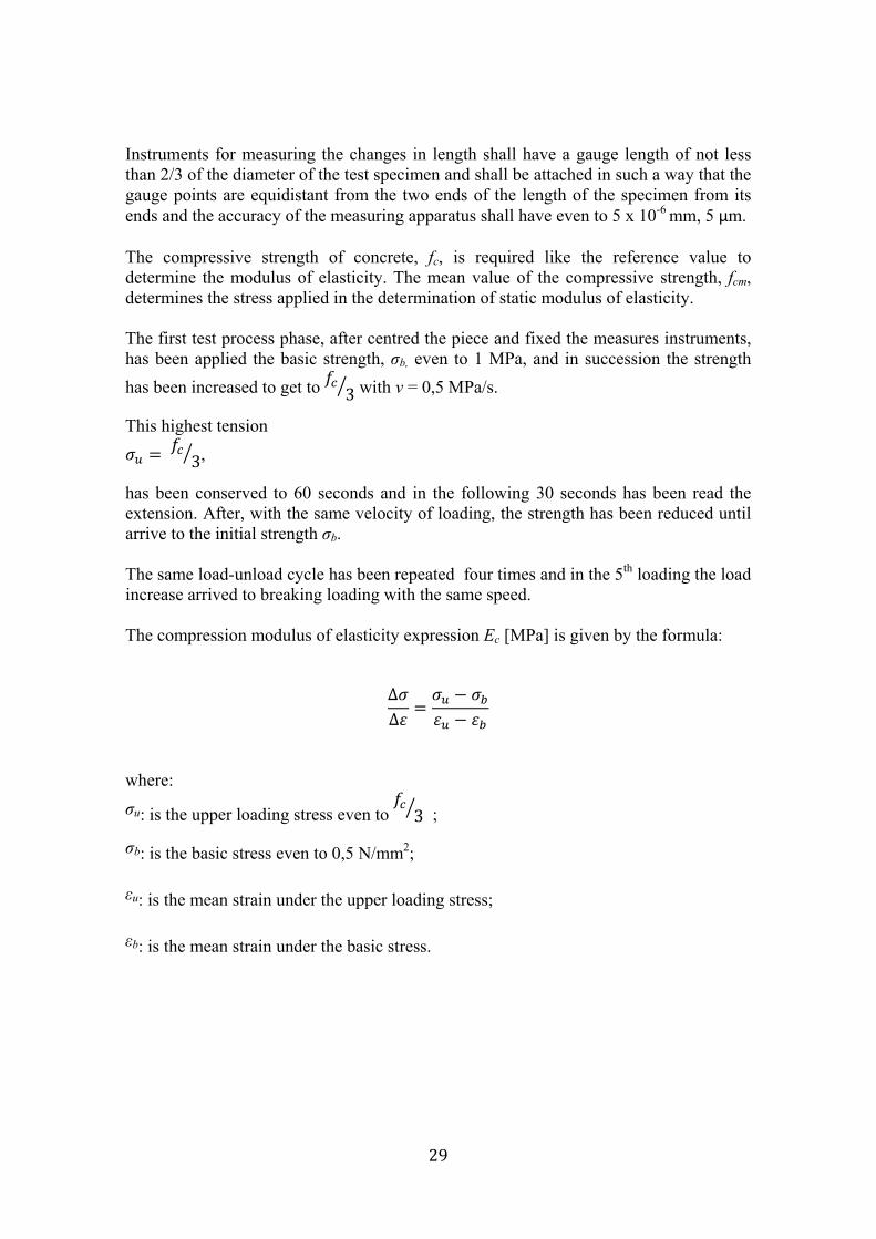
Instruments for measuring the changes in length shall have a gauge length of not less than 2/3 of the diameter of the test specimen and shall be attached in such a way that the gauge points are equidistant from the two ends of the length of the specimen from its ends and the accuracy of the measuring apparatus shall have even to 5 x 10-6 mm, 5 μm. The compressive strength of concrete, fc, is required like the reference value to determine the modulus of elasticity. The mean value of the compressive strength, fcm, determines the stress applied in the determination of static modulus of elasticity. The first test process phase, after centred the piece and fixed the measures instruments, has been applied the basic strength, σb, even to 1 MPa, and in succession the strength has been increased to get to 𝑓𝑐 3� with v = 0,5 MPa/s.

This highest tension 𝜎𝑢 = 𝑓𝑐 3� ,

has been conserved to 60 seconds and in the following 30 seconds has been read the extension. After, with the same velocity of loading, the strength has been reduced until arrive to the initial strength σb. The same load-unload cycle has been repeated four times and in the 5th loading the load increase arrived to breaking loading with the same speed. The compression modulus of elasticity expression Ec [MPa] is given by the formula:

∆𝜎∆𝜀

=𝜎𝑢 − 𝜎𝑏𝜀𝑢 − 𝜀𝑏

where: σu: is the upper loading stress even to 𝑓𝑐 3� ;

σb: is the basic stress even to 0,5 N/mm2; εu: is the mean strain under the upper loading stress; εb: is the mean strain under the basic stress.

30

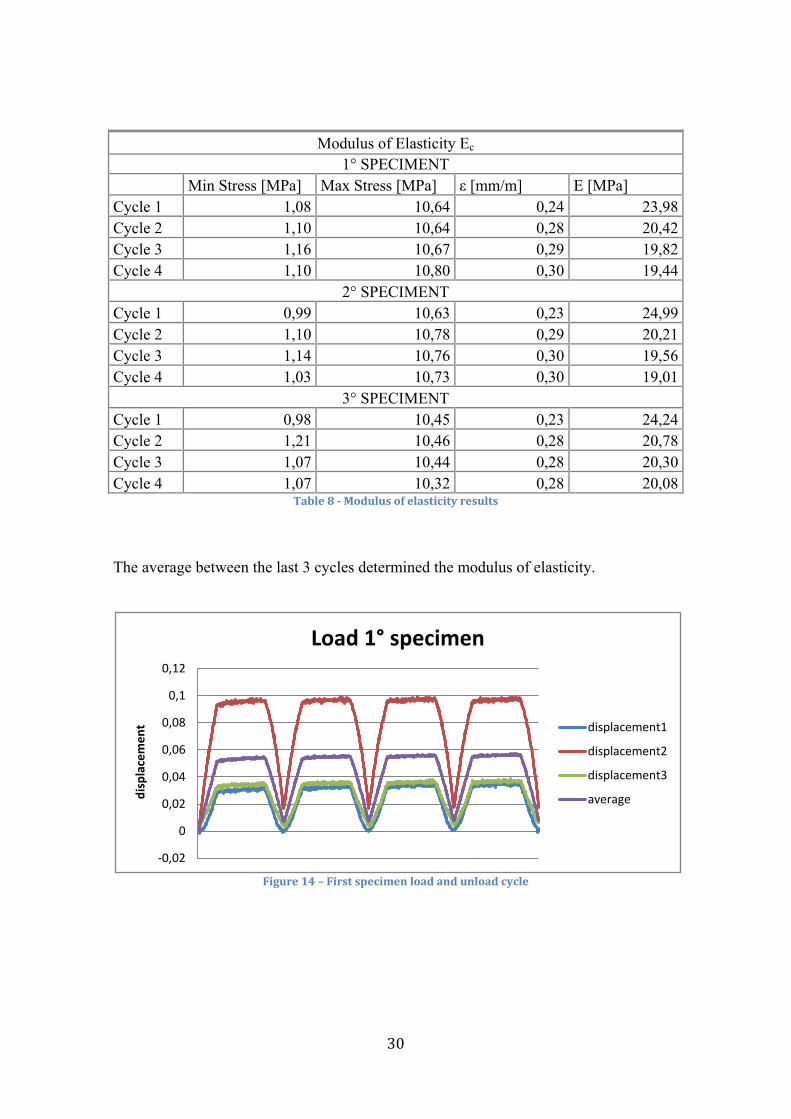
Modulus of Elasticity Ec

1° SPECIMENT Min Stress [MPa] Max Stress [MPa] ε [mm/m] E [MPa] Cycle 1 1,08 10,64 0,24 23,98 Cycle 2 1,10 10,64 0,28 20,42 Cycle 3 1,16 10,67 0,29 19,82 Cycle 4 1,10 10,80 0,30 19,44

2° SPECIMENT Cycle 1 0,99 10,63 0,23 24,99 Cycle 2 1,10 10,78 0,29 20,21 Cycle 3 1,14 10,76 0,30 19,56 Cycle 4 1,03 10,73 0,30 19,01

3° SPECIMENT Cycle 1 0,98 10,45 0,23 24,24 Cycle 2 1,21 10,46 0,28 20,78 Cycle 3 1,07 10,44 0,28 20,30 Cycle 4 1,07 10,32 0,28 20,08

Table 8 - Modulus of elasticity results

The average between the last 3 cycles determined the modulus of elasticity.

Figure 14 – First specimen load and unload cycle

-0,02

0

0,02

0,04

0,06

0,08

0,1

0,12

disp

lace

men

t

Load 1° specimen

displacement1

displacement2

displacement3

average

31

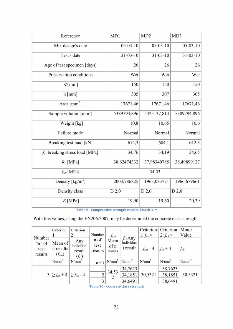
Reference MD1 MD2 MD3

Mix design's date 05-03-10 05-03-10 05-03-10

Test's date 31-03-10 31-03-10 31-03-10

Age of test specimen [days] 26 26 26

Preservation conditions Wet Wet Wet

Φ[mm] 150 150 150

h [mm] 305 307 305

Area [mm2] 17671,46 17671,46 17671,46

Sample volume [mm3] 5389794,896 5425137,814 5389794,896

Weight [kg] 10,8 10,65 10,6

Failure mode Normal Normal Normal

Breaking test load [kN] 614,3 604,1 612,3

fc breaking stress load [MPa] 34,76 34,19 34,65

Rc [MPa] 38,62474332 37,98340785 38,49899127

fcm [MPa] 34,53

Density [kg/m3] 2003,786825 1963,083771 1966,679661

Density class D 2,0 D 2,0 D 2,0

E [MPa] 19,90 19,60 20,39

Table 9 - Compressive strength results, March 31st

With this values, using the EN206:2007, may be determined the concrete class strength.

Number “n” of

test results

Criterion 1

Criterion 2 Number

n of test

results

fcm Mean of n

results

fci Any individual result

Criterion 1: fck ≤

Criterion 2: fck ≤

Minor Value

Mean of n results

(fcm)

Any individual

result (fci)

fcm - 4 fci + 4 fck

N/mm2 N/mm2 n = 3 N/mm2 N/mm2 N/mm2 N/mm2 N/mm2

3 ≥ fck + 4 ≥ fck - 4 1

34,532

34,7623 30,5321

38,7623 30,5321 2 34,1851 38,1851

3 34,6491 38,6491 Table 10 - Concrete class strength

32

The strength class of these LWC samples was higher than the reference normal concrete stress class C25/30; in fact the strength class of these specimens was LC 30/33, but the request strength class was LC 25/28 because, in the second part of the thesis, the scope is compare the failure mode of LWC composite slabs with NC composite slabs. This error is common because the mix-proportioning criteria of LWC is different to NC, in fact the absolute volume method:

𝑉 = �𝑊 + 𝐶𝑆𝑐

+𝑓𝑎𝑝𝑆𝑓𝑎

�10−3

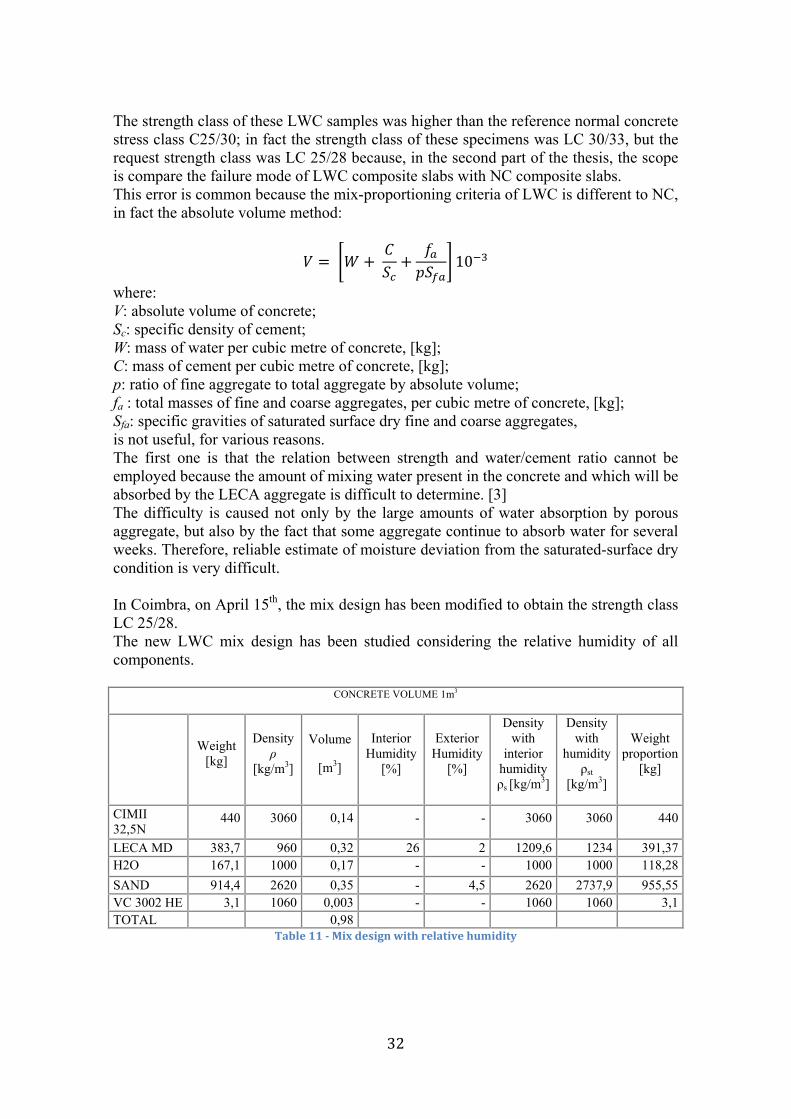
where: V: absolute volume of concrete; Sc: specific density of cement; W: mass of water per cubic metre of concrete, [kg]; C: mass of cement per cubic metre of concrete, [kg]; p: ratio of fine aggregate to total aggregate by absolute volume; fa : total masses of fine and coarse aggregates, per cubic metre of concrete, [kg]; Sfa: specific gravities of saturated surface dry fine and coarse aggregates, is not useful, for various reasons. The first one is that the relation between strength and water/cement ratio cannot be employed because the amount of mixing water present in the concrete and which will be absorbed by the LECA aggregate is difficult to determine. [3] The difficulty is caused not only by the large amounts of water absorption by porous aggregate, but also by the fact that some aggregate continue to absorb water for several weeks. Therefore, reliable estimate of moisture deviation from the saturated-surface dry condition is very difficult. In Coimbra, on April 15th, the mix design has been modified to obtain the strength class LC 25/28. The new LWC mix design has been studied considering the relative humidity of all components.

CONCRETE VOLUME 1m3

Weight [kg]

Density ρ

[kg/m3]

Volume

[m3]

Interior Humidity

[%]

Exterior Humidity

[%]

Density with

interior humidity ρs [kg/m3]

Density with

humidity ρst

[kg/m3]

Weight proportion

[kg]

CIMII 32,5N

440 3060 0,14 - - 3060 3060 440

LECA MD 383,7 960 0,32 26 2 1209,6 1234 391,37 H2O 167,1 1000 0,17 - - 1000 1000 118,28 SAND 914,4 2620 0,35 - 4,5 2620 2737,9 955,55 VC 3002 HE 3,1 1060 0,003 - - 1060 1060 3,1 TOTAL 0,98

Table 11 - Mix design with relative humidity

33

In this the table the total volume result is 0,98m3, because the remaining 0,20m3 is occupied by air.

The two columns concerning the interior and exterior humidity are basic to calculate the density with humidity with the following expression:

Density with interior humidity:

𝜌𝑠 = 𝜌 �1 +𝐻𝑖

100�

Density with humidity:

𝜌𝑠𝑡 = 𝜌 �1 +𝐻𝑖

100� �1 +

𝐻𝑒100�

The last column indicates the truth weight of all components considering the humidity: the only changes between the first and the last column concern the LECA, the water and the sand.

The weight proportion is calculated multiplicand the density with humidity and the volume and the real weight of water is calculated with the following expression:

𝑤′ = 𝑤 − �𝑆 × 𝜌 ×𝐻𝑒

100�𝑠𝑎𝑛𝑑− �𝐿 × 𝜌 × �1 +

𝐻𝑖100� �

𝐻𝑒100�

�𝐿𝐸𝐶𝐴

where:

w’: real weight of water,

w: water weight, before the humidity study,

S: sand volume,

L: LECA volume,

ρ: density,

Hi: interior humidity,

He: exterior humidity.

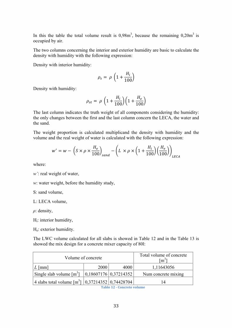
The LWC volume calculated for all slabs is showed in Table 12 and in the Table 13 is showed the mix design for a concrete mixer capacity of 80l:

Volume of concrete Total volume of concrete [m3]

L [mm] 2000 4000 1,11643056 Single slab volume [m3] 0,18607176 0,37214352 Num concrete mixing

4 slabs total volume [m3] 0,37214352 0,74428704 14 Table 12 - Concrete volume

34

MIX DESIGN 15/04/2010 [80L]

CIM II 32,5 N 35,2 [kg]

LECA MD 31,1 [kg]

H2O 9,45 [kg]

SAND 76,73 [kg]

VC 3002 HE 0,247 [kg]

Table 13 - Mix design 80l

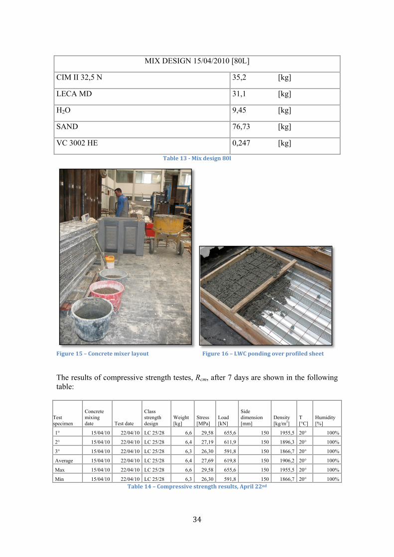
Figure 15 – Concrete mixer layout Figure 16 – LWC ponding over profiled sheet

The results of compressive strength testes, Rcm, after 7 days are shown in the following table:

Test specimen

Concrete mixing date Test date

Class strength design

Weight [kg]

Stress [MPa]

Load [kN]

Side dimension [mm]

Density [kg/m3]

T [°C]

Humidity [%]

1° 15/04/10 22/04/10 LC 25/28 6,6 29,58 655,6 150 1955,5 20° 100%

2° 15/04/10 22/04/10 LC 25/28 6,4 27,19 611,9 150 1896,3 20° 100%

3° 15/04/10 22/04/10 LC 25/28 6,3 26,30 591,8 150 1866,7 20° 100%

Average 15/04/10 22/04/10 LC 25/28 6,4 27,69 619,8 150 1906,2 20° 100%

Max 15/04/10 22/04/10 LC 25/28 6,6 29,58 655,6 150 1955,5 20° 100%

Min 15/04/10 22/04/10 LC 25/28 6,3 26,30 591,8 150 1866,7 20° 100% Table 14 – Compressive strength results, April 22nd

35

The same test has been done to calculate the LWC’s Rcm after 28 days:

Test specimen

Concrete mixing date Test date

Class strength design

Weight [kg]

Stress [MPa]

Load [kN]

Side dimension [mm]

Density [kg/m3]

T [°C]

Humidity [%]

1° 15/04/10 14/05/10 LC 25/28 6,3 33,13 745,52 150 1866,7 20° 100%

2° 15/04/10 14/05/10 LC 25/28 6,3 32,64 734,44 150 1866,7 20° 100%

3° 15/04/10 14/05/10 LC 25/28 6,1 30,45 685,06 150 1807,4 20° 100%

Average 15/04/10 14/05/10 LC 25/28 6,2 32,1 721,7 150 1866,7 20° 100%

Max 15/04/10 14/05/10 LC 25/28 6,3 33,1 745,5 150 1866,7 20° 100%

Min 15/04/10 14/05/10 LC 25/28 6,1 30,4 685,1 150 1866,7 20° 100% Table 15 – Compressive strength result, May 14th

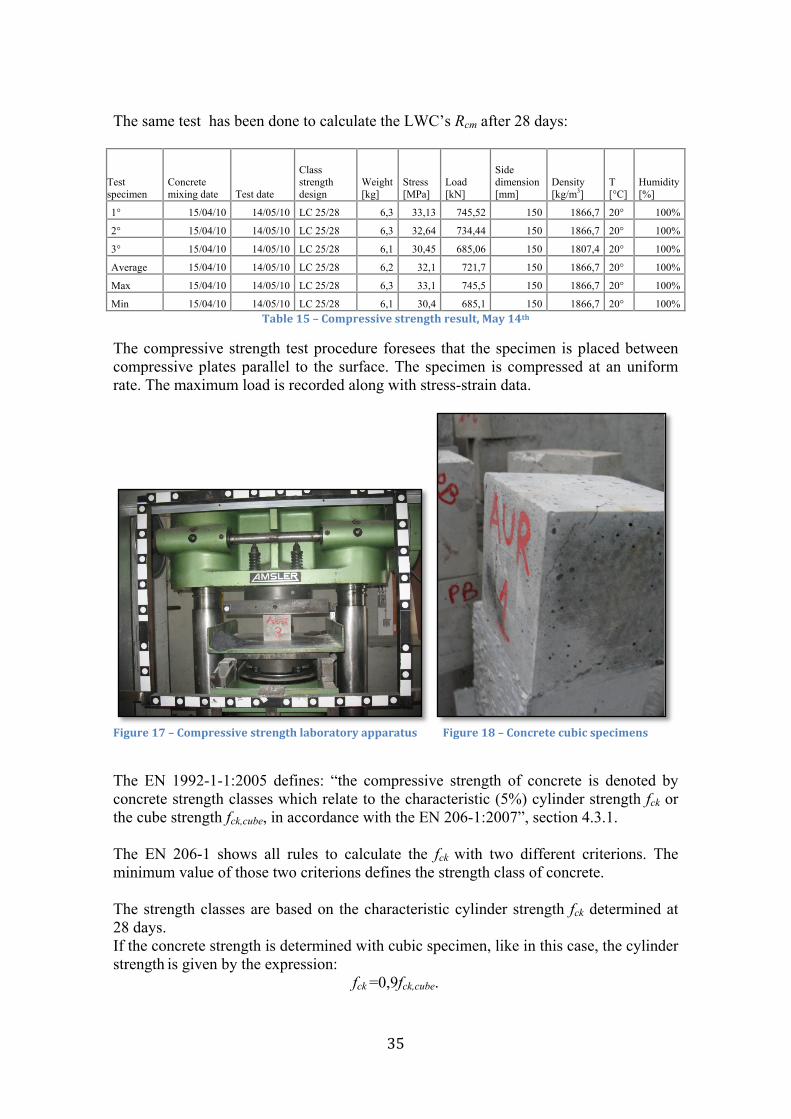
The compressive strength test procedure foresees that the specimen is placed between compressive plates parallel to the surface. The specimen is compressed at an uniform rate. The maximum load is recorded along with stress-strain data.

Figure 17 – Compressive strength laboratory apparatus Figure 18 – Concrete cubic specimens

The EN 1992-1-1:2005 defines: “the compressive strength of concrete is denoted by concrete strength classes which relate to the characteristic (5%) cylinder strength fck or the cube strength fck,cube, in accordance with the EN 206-1:2007”, section 4.3.1. The EN 206-1 shows all rules to calculate the fck with two different criterions. The minimum value of those two criterions defines the strength class of concrete. The strength classes are based on the characteristic cylinder strength fck determined at 28 days. If the concrete strength is determined with cubic specimen, like in this case, the cylinder strength is given by the expression:

fck =0,9fck,cube.

36

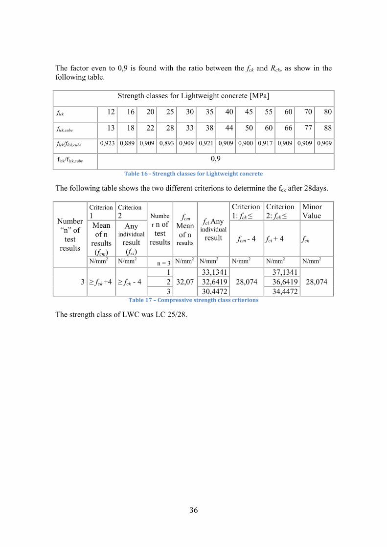
The factor even to 0,9 is found with the ratio between the fck and Rck, as show in the following table.

Strength classes for Lightweight concrete [MPa]

flck 12 16 20 25 30 35 40 45 55 60 70 80

flck,cube 13 18 22 28 33 38 44 50 60 66 77 88

flck/flck,cube 0,923 0,889 0,909 0,893 0,909 0,921 0,909 0,900 0,917 0,909 0,909 0,909

flck/flck,cube 0,9

Table 16 - Strength classes for Lightweight concrete

The following table shows the two different criterions to determine the fck after 28days.

Number “n” of

test results

Criterion 1

Criterion 2 Numbe

r n of test

results

fcm Mean of n

results

fci Any individual

result

Criterion 1: fck ≤

Criterion 2: fck ≤

Minor Value

Mean of n

results (fcm)

Any individual

result (fci)

fcm - 4 fci + 4 fck

N/mm2 N/mm2 n = 3 N/mm2 N/mm2 N/mm2 N/mm2 N/mm2

3 ≥ fck +4 ≥ fck - 4 1

32,07 33,1341

28,074 37,1341

28,074 2 32,6419 36,6419 3 30,4472 34,4472

Table 17 – Compressive strength class criterions

The strength class of LWC was LC 25/28.

37

Composite slabs:

General Notions In this section is made a widen approach of the section 9 of EN 1994-1-1:2005 about the composite slabs with profiled steel sheeting for building.

The general scope of section 9 deals with composite floor slabs spanning only in the direction of the ribs.

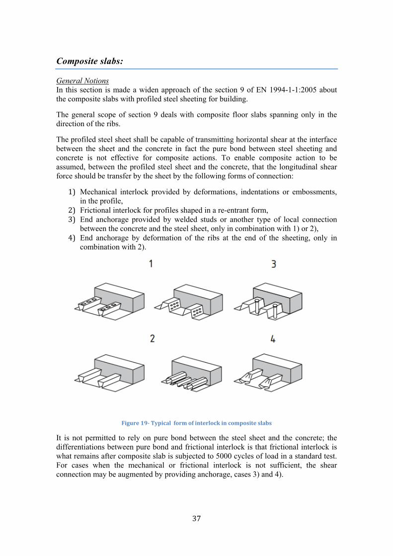
The profiled steel sheet shall be capable of transmitting horizontal shear at the interface between the sheet and the concrete in fact the pure bond between steel sheeting and concrete is not effective for composite actions. To enable composite action to be assumed, between the profiled steel sheet and the concrete, that the longitudinal shear force should be transfer by the sheet by the following forms of connection:

1) Mechanical interlock provided by deformations, indentations or embossments, in the profile,

2) Frictional interlock for profiles shaped in a re-entrant form, 3) End anchorage provided by welded studs or another type of local connection

between the concrete and the steel sheet, only in combination with 1) or 2), 4) End anchorage by deformation of the ribs at the end of the sheeting, only in

combination with 2).

Figure 19- Typical form of interlock in composite slabs

It is not permitted to rely on pure bond between the steel sheet and the concrete; the differentiations between pure bond and frictional interlock is that frictional interlock is what remains after composite slab is subjected to 5000 cycles of load in a standard test. For cases when the mechanical or frictional interlock is not sufficient, the shear connection may be augmented by providing anchorage, cases 3) and 4).

38

The minimum design slab thicknesses, recommended in EN 1994-1-1, are classified in two different classes on the basis of the slab-beam behaviour show in the following table:

Compositely slab-beam behaviour or diaphragm

use

No-compositely slab-beam behaviour or no stabilising

function

Overall depth of the slab h ≥ 90 mm h ≥ 80 mm

Thickness of concrete above the main flat surface of the top of the ribs of the sheeting hc ≥ 50 mm hc ≥ 40 mm

Table 18 – Slab-beam behaviour

It is generally useful to provide reinforcement in the concrete slab for the following reasons:

- Load distribution of line or point loads; - Local reinforcement of slab openings; - Fire resistance; - Upper reinforcement in hogging moment area; - To control cracking due to shrinkage.

Mesh reinforcement may be placed at the top of the profiled decking ribs. Length of, and cover to, reinforcement should satisfy the usual requirements for reinforced concrete, to be more precise:

- Transverse and longitudinal reinforcement shall be provide within the depth hc of the concrete;

- The amount of reinforcement in both directions should be not less than 80mm2/m, which is based on the smallest value of hc and the minimum percentage of crack-control reinforcement for unpropped construction;

- The spacing of the reinforcement bars should not exceed 2h and 350mm, whichever is the lesser.

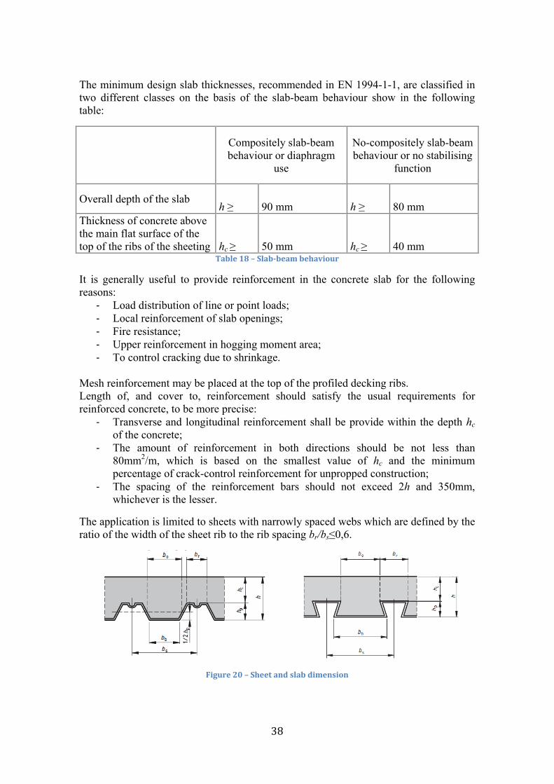
The application is limited to sheets with narrowly spaced webs which are defined by the ratio of the width of the sheet rib to the rib spacing br/bs≤0,6.

Figure 20 – Sheet and slab dimension

39

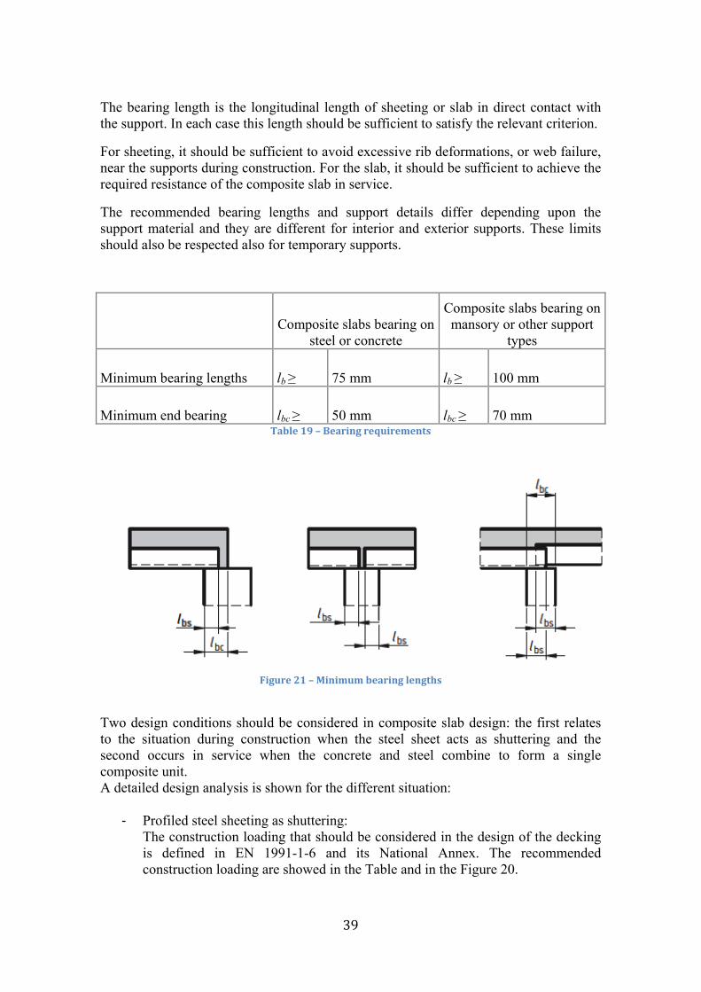
The bearing length is the longitudinal length of sheeting or slab in direct contact with the support. In each case this length should be sufficient to satisfy the relevant criterion.

For sheeting, it should be sufficient to avoid excessive rib deformations, or web failure, near the supports during construction. For the slab, it should be sufficient to achieve the required resistance of the composite slab in service.

The recommended bearing lengths and support details differ depending upon the support material and they are different for interior and exterior supports. These limits should also be respected also for temporary supports.

Composite slabs bearing on

steel or concrete

Composite slabs bearing on mansory or other support

types

Minimum bearing lengths lb ≥ 75 mm lb ≥ 100 mm

Minimum end bearing lbc ≥ 50 mm lbc ≥ 70 mm Table 19 – Bearing requirements

Figure 21 – Minimum bearing lengths

Two design conditions should be considered in composite slab design: the first relates to the situation during construction when the steel sheet acts as shuttering and the second occurs in service when the concrete and steel combine to form a single composite unit. A detailed design analysis is shown for the different situation:

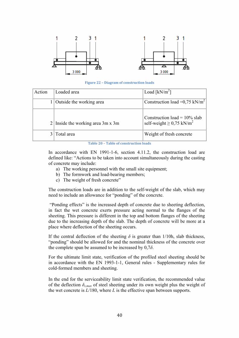
- Profiled steel sheeting as shuttering: The construction loading that should be considered in the design of the decking is defined in EN 1991-1-6 and its National Annex. The recommended construction loading are showed in the Table and in the Figure 20.

40

Figure 22 – Diagram of construction loads

Action Loaded area Load [kN/m2]

1 Outside the working area Construction load =0,75 kN/m2

2 Inside the working area 3m x 3m Construction load = 10% slab self-weight ≥ 0,75 kN/m2

3 Total area Weight of fresh concrete

Table 20 – Table of construction loads

In accordance with EN 1991-1-6, section 4.11.2, the construction load are defined like: “Actions to be taken into account simultaneously during the casting of concrete may include:

a) The working personnel with the small site equipment; b) The formwork and load-bearing members; c) The weight of fresh concrete”

The construction loads are in addition to the self-weight of the slab, which may need to include an allowance for “ponding” of the concrete.

“Ponding effects” is the increased depth of concrete due to sheeting deflection, in fact the wet concrete exerts pressure acting normal to the flanges of the sheeting. This pressure is different in the top and bottom flanges of the sheeting due to the increasing depth of the slab. The depth of concrete will be more at a place where deflection of the sheeting occurs.

If the central deflection of the sheeting δ is greater than 1/10h, slab thickness, “ponding” should be allowed for and the nominal thickness of the concrete over the complete span be assumed to be increased by 0,7δ.

For the ultimate limit state, verification of the profiled steel sheeting should be in accordance with the EN 1993-1-1, General rules - Supplementary rules for cold-formed members and sheeting. In the end for the serviceability limit state verification, the recommended value of the deflection δs,max of steel sheeting under its own weight plus the weight of the wet concrete is L/180, where L is the effective span between supports.

41

In the end the requirement for verification of the profiled sheeting at serviceability limit states is expressed in term of the deflection under the weight of the wet concrete and is no requirement to check that such deflection should be elastic.

- Composite slab: Composite slab design verification is required for the floor slab after composite behaviour has hardened and any props have been removed. The actions on the composite slab should be in accordance with EN 1991-1-1. At the ULS, ultimate limit states, the following analysis methods may be used for the composite slabs: a) Linear-elastic analysis:

i. without moment redistribution: at internal supports if cracking effects are considered;

ii. with moment redistribution: at internal supports (limited to 30%) without considering concrete cracking effects.

b) Rigid plastic global analysis provided that is shown that the sections where plastic rotations are required have sufficient rotation capacity;

c) Elastic-plastic analysis, taking into account the non-linear material properties.

Linear methods of analysis should be used for the SLS too.

Before to show the ultimate limit states behaviour of composite slabs is better deal with composite behaviour, that which occurs when the steel sheeting plus any additional reinforcement and hardened concrete have combined to form a single structural element.

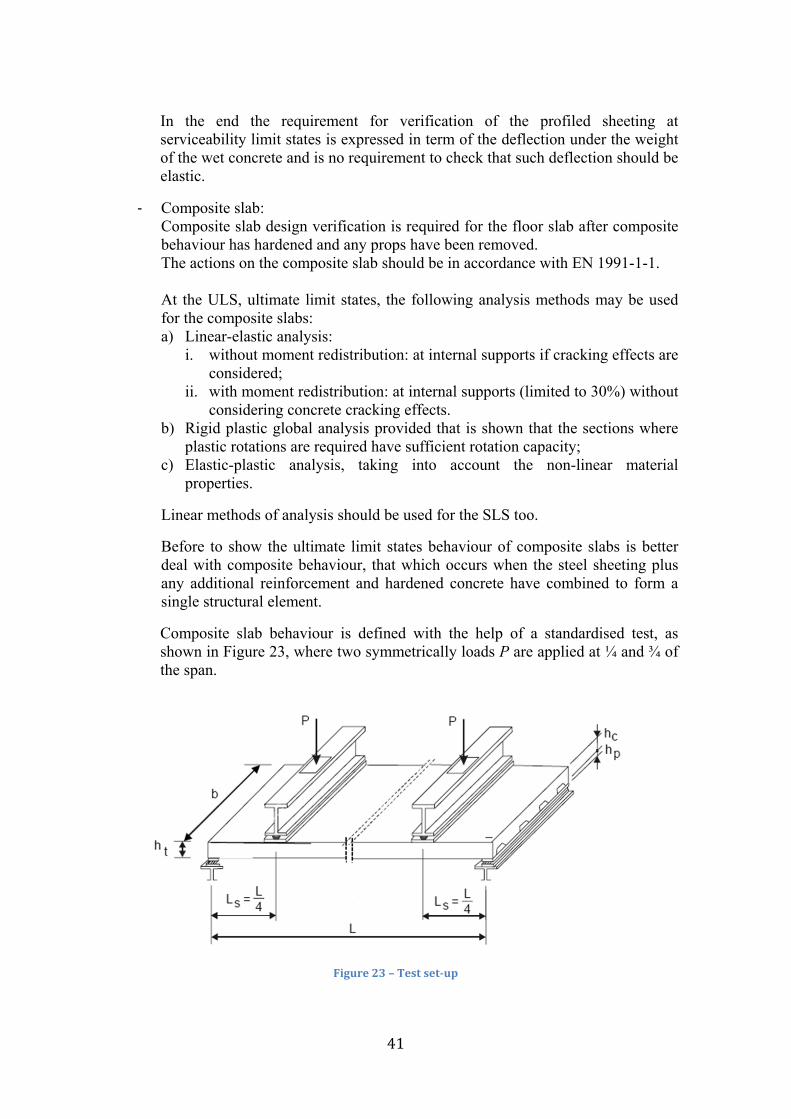
Composite slab behaviour is defined with the help of a standardised test, as shown in Figure 23, where two symmetrically loads P are applied at ¼ and ¾ of the span.

Figure 23 – Test set-up

42

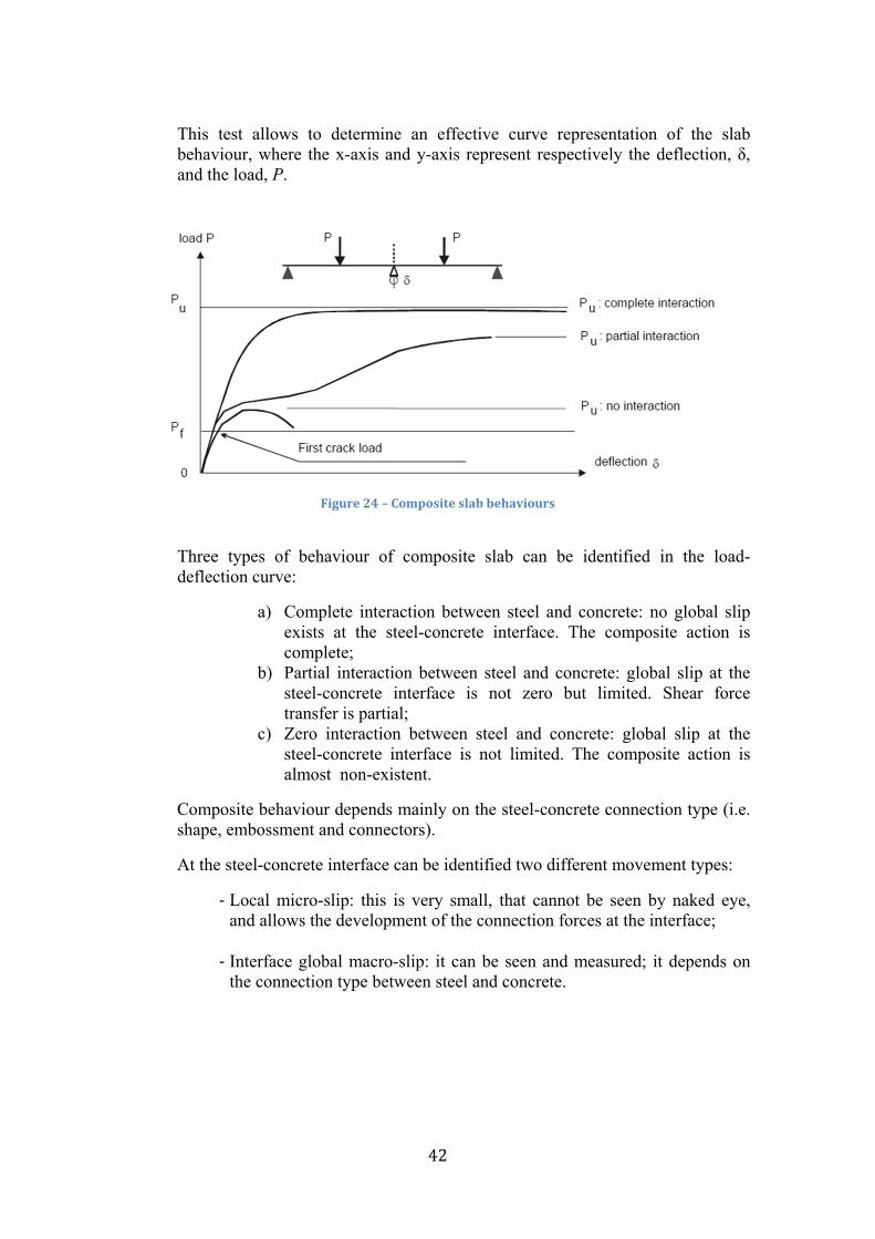
This test allows to determine an effective curve representation of the slab behaviour, where the x-axis and y-axis represent respectively the deflection, δ, and the load, P.

Figure 24 – Composite slab behaviours

Three types of behaviour of composite slab can be identified in the load-deflection curve:

a) Complete interaction between steel and concrete: no global slip exists at the steel-concrete interface. The composite action is complete;

b) Partial interaction between steel and concrete: global slip at the steel-concrete interface is not zero but limited. Shear force transfer is partial;

c) Zero interaction between steel and concrete: global slip at the steel-concrete interface is not limited. The composite action is almost non-existent.

Composite behaviour depends mainly on the steel-concrete connection type (i.e. shape, embossment and connectors).

At the steel-concrete interface can be identified two different movement types:

- Local micro-slip: this is very small, that cannot be seen by naked eye, and allows the development of the connection forces at the interface;

- Interface global macro-slip: it can be seen and measured; it depends on the connection type between steel and concrete.

43

Three types of bond exist between steel and concrete:

- Physical-chemical bond which is always low but exists for all profiles; this phenomena accounts for most of the initial bond, from 0 to Pf;

- Friction bond which develops as soon as micro slip appear; - Mechanical anchorage bond which acts after the first slip and depends on

the steel-concrete interface shape.

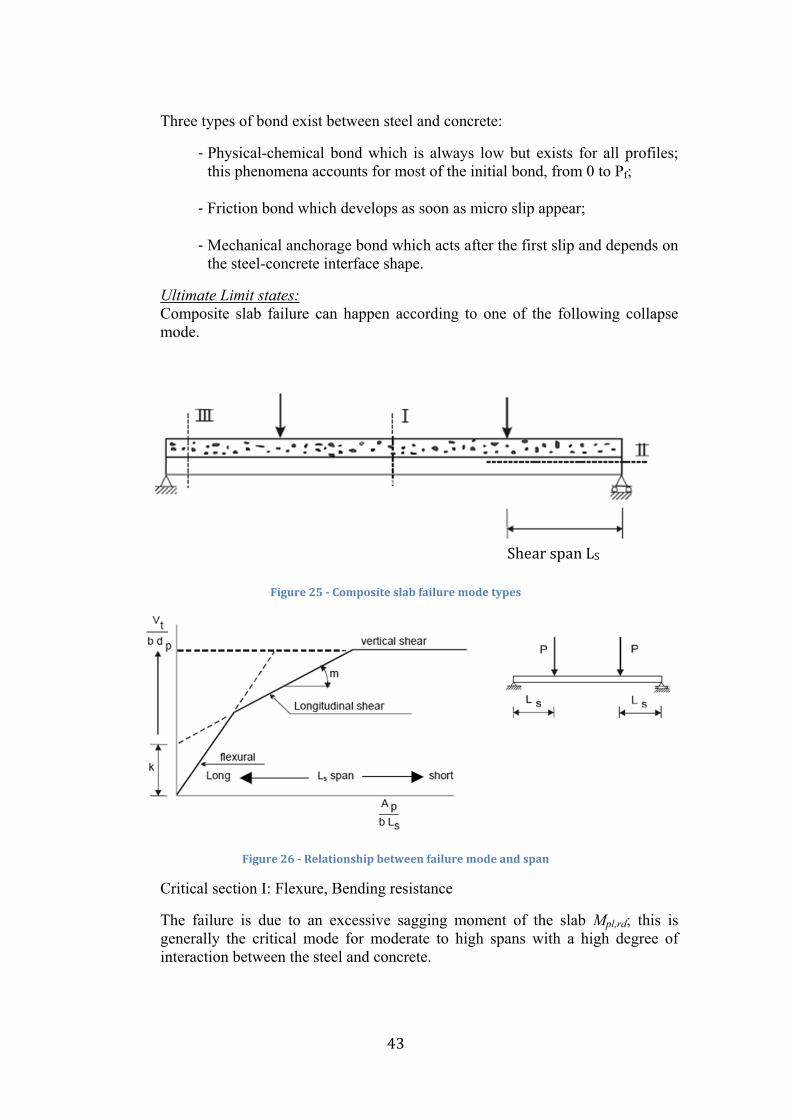
Ultimate Limit states: Composite slab failure can happen according to one of the following collapse mode.

Figure 25 - Composite slab failure mode types

Figure 26 - Relationship between failure mode and span

Critical section I: Flexure, Bending resistance

The failure is due to an excessive sagging moment of the slab Mpl,rd; this is generally the critical mode for moderate to high spans with a high degree of interaction between the steel and concrete.

Shear span LS

44

Flexural failure occurs when the plastic capacity of the slab is reached. This is possible if the resistance for the longitudinal shear transfer in the shear span is large enough to allow yielding of the entire cross section of the sheeting. This section can be critical if there is complete shear connection at the interface between the sheet and the concrete. In other words, it means the bond provides full interaction.

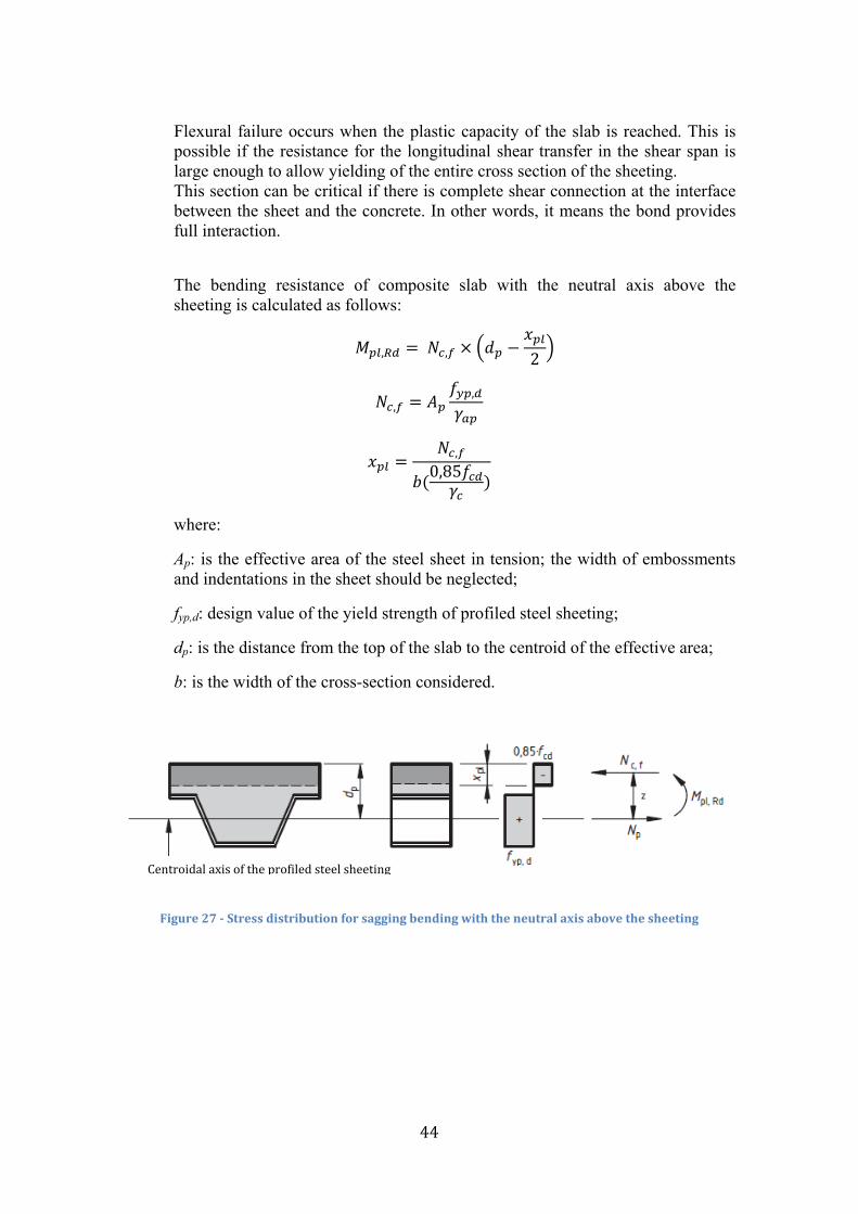
The bending resistance of composite slab with the neutral axis above the sheeting is calculated as follows:

𝑀𝑝𝑙,𝑅𝑑 = 𝑁𝑐,𝑓 × �𝑑𝑝 −𝑥𝑝𝑙2�

𝑁𝑐,𝑓 = 𝐴𝑝𝑓𝑦𝑝,𝑑

𝛾𝑎𝑝

𝑥𝑝𝑙 =𝑁𝑐,𝑓

𝑏(0,85𝑓𝑐𝑑𝛾𝑐

)

where:

Ap: is the effective area of the steel sheet in tension; the width of embossments and indentations in the sheet should be neglected;

fyp,d: design value of the yield strength of profiled steel sheeting;

dp: is the distance from the top of the slab to the centroid of the effective area;

b: is the width of the cross-section considered.

Figure 27 - Stress distribution for sagging bending with the neutral axis above the sheeting

Centroidal axis of the profiled steel sheeting

45

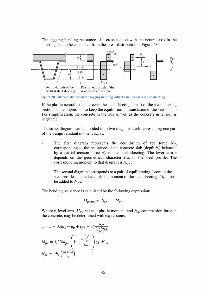
The sagging bending resistance of a cross-section with the neutral axis in the sheeting should be calculated from the stress distribution in Figure 28:

Figure 28 - Stress distribution for sagging bending with the neutral axis in the sheeting

If the plastic neutral axis intercepts the steel sheeting, a part of the steel sheeting section is in compression to keep the equilibrium in translation of the section. For simplification, the concrete in the ribs as well as the concrete in tension is neglected. The stress diagram can be divided in to two diagrams each representing one part of the design resistant moment MpsRd: - The first diagram represents the equilibrium of the force Ncf,

corresponding to the resistance of the concrete slab (depth hc) balanced by a partial tension force Np in the steel sheeting. The lever arm z depends on the geometrical characteristics of the steel profile. The corresponding moment to that diagram is Ncf z;

- The second diagram corresponds to a pair of equilibrating forces in the steel profile. The reduced plastic moment of the steel sheeting, Mpr , must be added to Ncf z.

The bending resistance is calculated by the following expression:

𝑀𝑝𝑠,𝑅𝑑 = 𝑁𝑐𝑓𝑧 + 𝑀𝑝𝑟 Where z, level arm, Mpr, reduced plastic moment, and Ncf, compression force in the concrete, may be determined with expressions:

𝑧 = ℎ − 0,5ℎ𝑐 − 𝑒𝑝 + (𝑒𝑝 − 𝑒) 𝑁𝑐𝑓𝐴𝑝𝑒𝑓𝑦𝑝,𝑑

𝛾𝑎𝑝

𝑀𝑝𝑟 = 1,25𝑀𝑝𝑎 �1 −𝑁𝑐𝑓

𝐴𝑝𝑓𝑦𝑝,𝑑

𝛾𝑎𝑝� ≤ 𝑀𝑝𝑎

𝑁𝑐𝑓 = 𝑏ℎ𝑐 �0,85𝑓𝑐𝑑

𝛾𝑐�

Centroidal axis of the profiled steel sheeting

Plastic neutral axis of the profiled steel sheeting

46

with:

ep: distance of the plastic neutral axis of the effective area of the sheeting to its underside;

e: distance from the centroidal axis of profiled steel sheeting to the extreme fibre of the composite slab in tension.

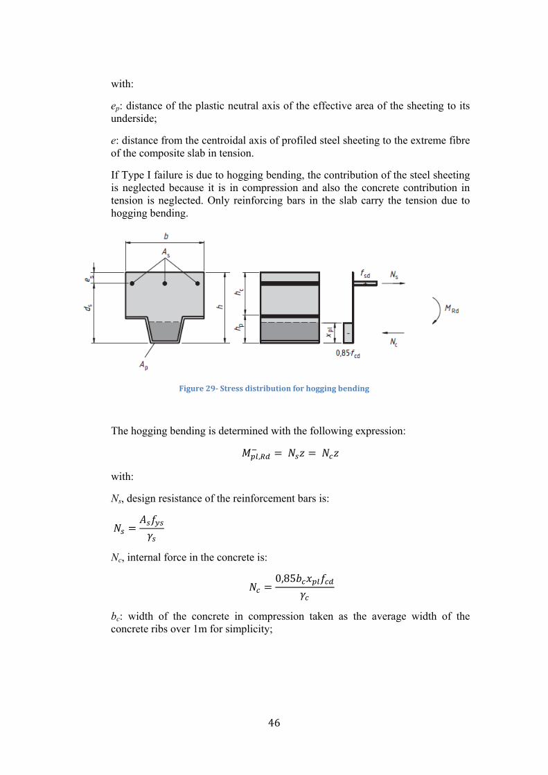
If Type I failure is due to hogging bending, the contribution of the steel sheeting is neglected because it is in compression and also the concrete contribution in tension is neglected. Only reinforcing bars in the slab carry the tension due to hogging bending.

Figure 29- Stress distribution for hogging bending

The hogging bending is determined with the following expression:

𝑀𝑝𝑙,𝑅𝑑− = 𝑁𝑠𝑧 = 𝑁𝑐𝑧

with:

Ns, design resistance of the reinforcement bars is:

𝑁𝑠 =𝐴𝑠𝑓𝑦𝑠𝛾𝑠

Nc, internal force in the concrete is:

𝑁𝑐 =0,85𝑏𝑐𝑥𝑝𝑙𝑓𝑐𝑑

𝛾𝑐

bc: width of the concrete in compression taken as the average width of the concrete ribs over 1m for simplicity;

47

xpl, depth of concrete in compression:

𝑥𝑝𝑙 = 𝐴𝑠𝑓𝑦𝑠𝛾𝑠

0,85𝑏𝑐𝑓𝑐𝑑𝛾𝑐

z, level arm of the resulting internal forces Nc and Ns:

𝑧 = 𝑑𝑠 −𝑥𝑝𝑙2

Critical section II: Longitudinal shear

Failure in longitudinal shear is indicated by relative movement, end slip, between the sheeting and the concrete at the end of the test specimen at a load lower than the load, which would cause flexural bending failure. Longitudinal shear failure occurs if the shear span is not sufficiently long for the mechanical interlocking strength to develop the plastic resistance. The resistance of shear connection determines the maximum load on the slab. The ultimate moment of resistance MP, Rd at section I cannot be reached. The design resistance against longitudinal shear should be determined by two different experimental methods: - m-k Method; - Partial connection Method. Both methods rely on tests on composite slabs to evaluate the shear connection and the test results are presented in terms of empirical constants, either m and k or τ. As far as slab design is concerned, the structural designer will not undertake tests to determine the m and k or τ factors; these constants are used by the decking manufacturers themselves in order to present designers with a range of load-span table for uniformly loaded conditions for their specific products. Designers should take care to ensure that they do not use this information for situations that are not covered by the scope of the testing especially if concentrated line or point loads are applied to the slab. From the load-deflection curve recorded from tests, the composite slab behaviour is classified as ductile or brittle. Ductility is the ability of a member to continue to deform while maintaining its load carrying capacity. The longitudinal shear behaviour may be considered ductile if the failure load exceeds the load causing a recorded end slip of 0,1mm by more than 10%; it means the mechanical interlock can provide greater bond effect than the chemical bond. If the maximum load is reached at a mid-span deflection exceeding L/50, the failure load should be taken at the mid-span deflection of L/50. Otherwise the behaviour is classified as brittle. Brittle behaviour is characterised by a significant decrease in load.

48

Moreover the load will never attain its maximum value again. This behaviour is due to the fact that the mechanical interlock is not able to ensure bond greater than the chemical bond and failure occurs by longitudinal shear. m-k Method without end anchorage:

The rules are based on the work by Porter and Eckberg, 1976. As implied by the name, the m-k method is based on establishing the gradient and the intercept of a linear relationship evaluated from two groups of three full-scale composite slab tests.

This method uses the vertical shear force Vt to check the longitudinal shear failure along the shear span Ls. The direct relationship between the vertical shear and the longitudinal shear is only known for elastic behaviour, if the behaviour is elastic-plastic, the relationship is not simple and the m-k method is used.

The m-k method is a semi-empirical approach, it does not have a definite physical representation and cannot be related directly to the shear bond, then m and k factors do not have a direct physical significance and they are simply empirical constants.

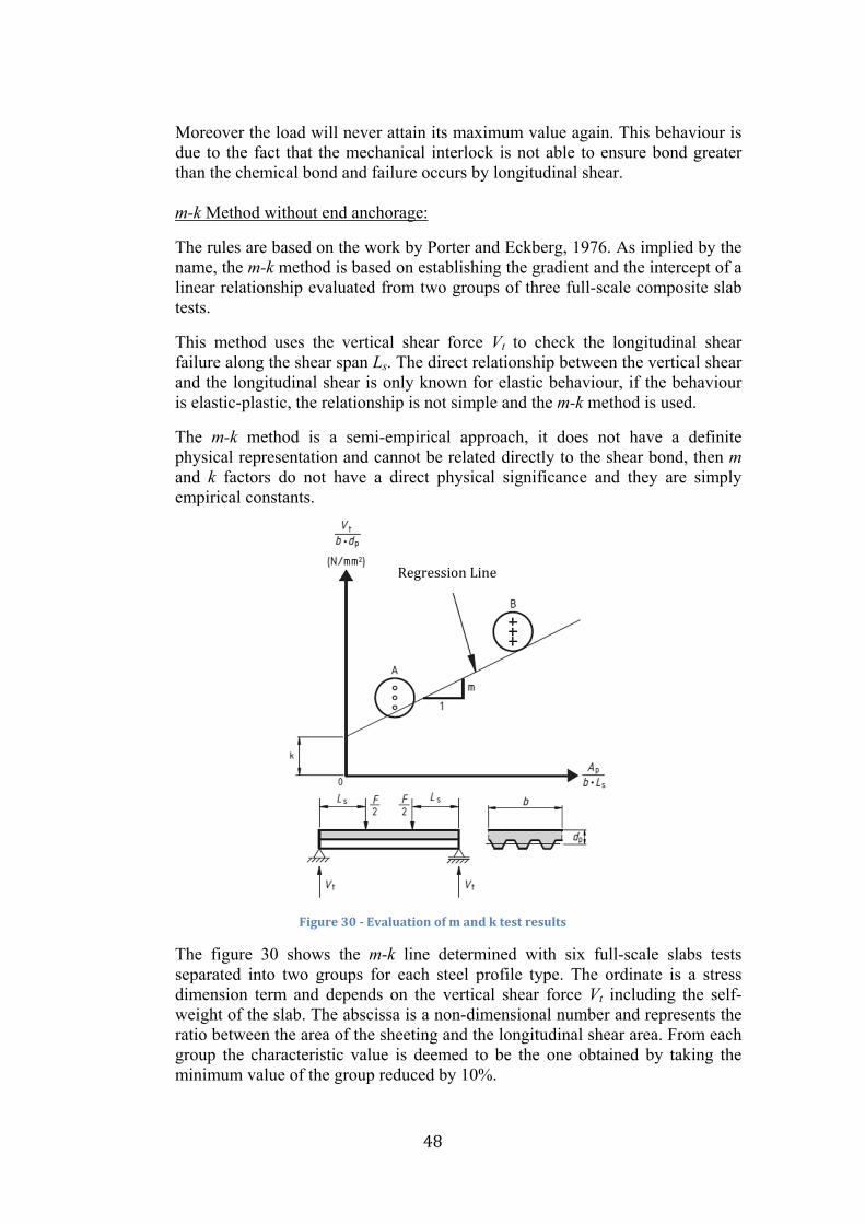
Figure 30 - Evaluation of m and k test results

The figure 30 shows the m-k line determined with six full-scale slabs tests separated into two groups for each steel profile type. The ordinate is a stress dimension term and depends on the vertical shear force Vt including the self-weight of the slab. The abscissa is a non-dimensional number and represents the ratio between the area of the sheeting and the longitudinal shear area. From each group the characteristic value is deemed to be the one obtained by taking the minimum value of the group reduced by 10%.

Regression Line

49

The design relationship is formed by the straight line, the so called “regression line”, through these characteristic values for groups A and B.

The design value of the resistance to shear for the composite slab is given by:

𝑉𝑙,𝑅𝑑 =𝑏𝑑𝑝𝛾𝑉𝑆

�𝑚𝐴𝑝𝑏𝐿𝑠

+ 𝑘�

For design, Ls depends on the type of loading. For a uniform load applied to the entire span L of a simply supported beam, equals L/4. This value is obtained by equating the area under shear force diagram for the uniformly distributed load to that due to a symmetrical two points load system applied at distance Ls from the supports. For other loading arrangement, Ls is obtained by similar assessment. Where the composite slab is designed as continuous, it is permitted to use an equivalent simple span between points of contraflexure for the determination of shear resistance. For end spans, however, the full exterior span length should be used in design.

Composite slab

Ls Simple supported

Continuous span

Internal span External span

L/4 0,8L 0,9L Table 21 - Span length

Partial connection method without end anchorage:

The rules in this section of EN 1994-1-1 are primarily based on the research by Stark and Brekelmans. As implied by the name, the partial connection method is based on establishing the amount of shear connection between the concrete and the sheet for given bending resistance. The bending resistance of the composite slab is based on simple plastic theory using rectangular stress block for the concrete and profiled steel sheeting. It is also assumed that, before the maximum moment is reached, there is a complete redistribution of longitudinal shear stress at the interface between the sheet and the concrete such that a mean value for the longitudinal shear strength τu can be calculated. This method should be used only for composite slabs with ductile behaviour. The design bending moment resistance MRd should be determined with the same conditions show in the critical section I, but with Ncf replaced by Nc and z replaced with z’.

𝑁𝑐 = 𝜏𝑢,𝑅𝑑𝑏𝐿𝑥

𝑧′ = 𝑧′ = ℎ − 0,5𝑥𝑝𝑙 − 𝑒𝑝 + �𝑒𝑝 − 𝑒�𝑁𝑐

𝐴𝑝𝑒𝑓𝑦𝑝.𝑑

50

where: τu,Rd: is the design shear strength �𝜏𝑢,𝑅𝑘

𝛾𝑉𝑠� obtained from slab tests meeting the

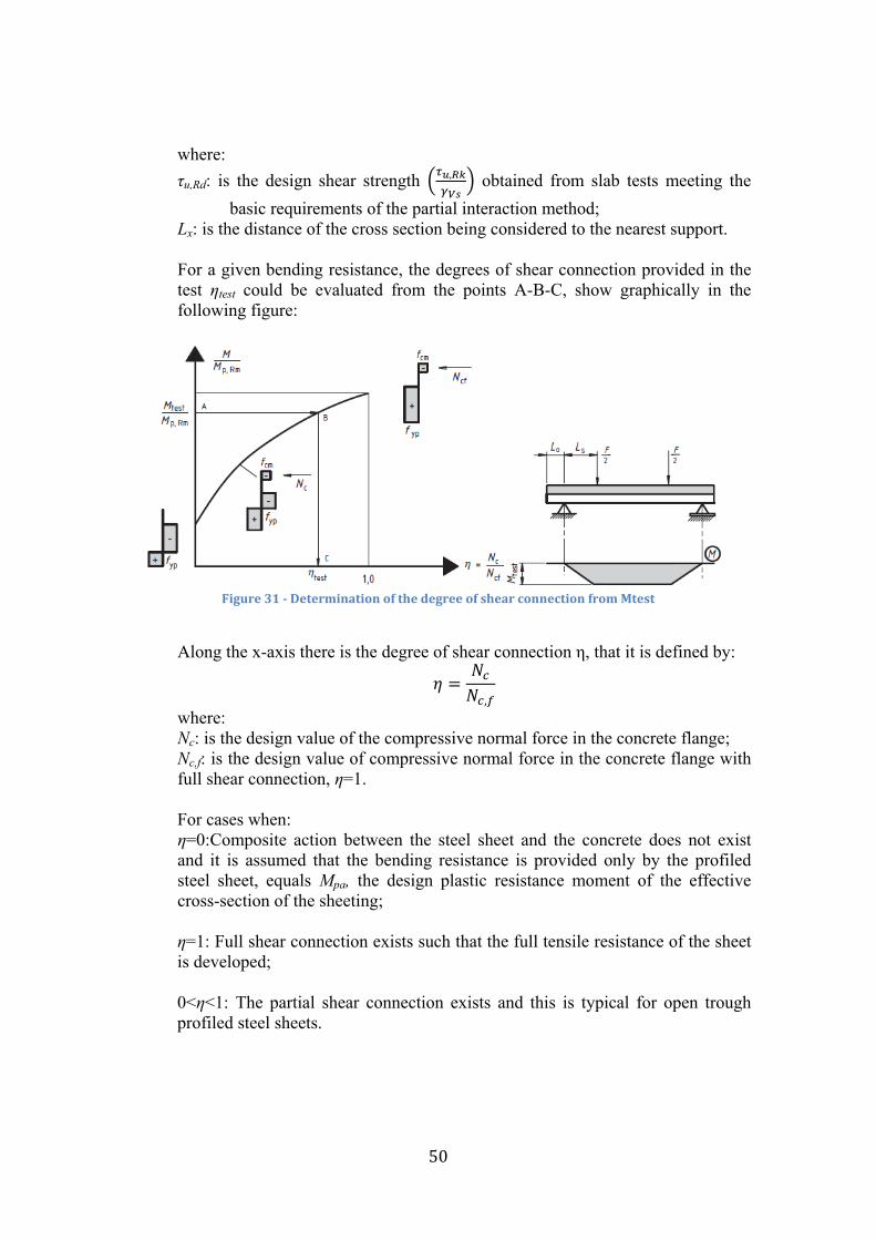
basic requirements of the partial interaction method; Lx: is the distance of the cross section being considered to the nearest support. For a given bending resistance, the degrees of shear connection provided in the test ηtest could be evaluated from the points A-B-C, show graphically in the following figure:

Figure 31 - Determination of the degree of shear connection from Mtest

Along the x-axis there is the degree of shear connection η, that it is defined by:

𝜂 =𝑁𝑐𝑁𝑐,𝑓

where: Nc: is the design value of the compressive normal force in the concrete flange;

Nc,f: is the design value of compressive normal force in the concrete flange with full shear connection, η=1. For cases when: η=0:Composite action between the steel sheet and the concrete does not exist and it is assumed that the bending resistance is provided only by the profiled steel sheet, equals Mpa, the design plastic resistance moment of the effective cross-section of the sheeting; η=1: Full shear connection exists such that the full tensile resistance of the sheet is developed; 0<η<1: The partial shear connection exists and this is typical for open trough profiled steel sheets.

51

To find the longitudinal shear strength τu it is possible analyse two different situation: - without the support reaction contribution:

𝜏𝑢 = 𝜂𝑡𝑒𝑠𝑡𝑁𝑐𝑓𝑏(𝐿𝑠 + 𝐿𝑜)

- with the support reaction contribution:

𝜏𝑢 = 𝜂𝑡𝑒𝑠𝑡𝑁𝑐𝑓 − 𝜇𝑉𝑡𝑏(𝐿𝑠 + 𝐿𝑜)

where: Lo: is the length of the overhang; μ: is the default value of the friction coefficient to be taken as 0,5; Vt: is the support reaction under the ultimate test load. In the end the characteristic shear strength τu,Rk should be calculated from the test values as the 5% fractile using an appropriate statistical model, in accordance with EN 1990, Annex D section 7.2.

End anchorage:

In this section only rules for through-deck welded studs are provided, because the design resistance against longitudinal shear of slabs with the end anchorage, 3) and 4) show in the figure 19 may be determined by the partial connection method with Nc increased by the design resistance of the end anchorage.

The design resistance of a headed stud welded trough the steel sheet used for end anchorage should be taken as the smaller of the design shear resistance of a headed stud welded, PRd, and the design value of the bearing resistance of a stud, Ppb,Rd.

𝑃𝑝𝑏,𝑅𝑑 = min (𝑃𝑅𝑑; 𝑃𝑝𝑏,𝑅𝑑)

In accordance with the section 6.6.3.1 of EN 1994-1-1, PRd should be determined from:

𝑃𝑅𝑑 = 0,8𝑓𝑢𝜋𝑑2/4𝛾𝑉

or:

𝑃𝑅𝑑 =0,29𝛼𝑑2�𝑓𝑐𝑘𝐸𝑐𝑚

𝛾𝑉

52

whichever is smaller, whit:

𝛼 = 0,2 �ℎ𝑠𝑐𝑑

+ 1� for 3 ≤ ℎ𝑠𝑐𝑑≤ 4

𝛼 = 1 for ℎ𝑠𝑐𝑑

> 4

where:

d: is the diameter of the shank of the stud,

hsc: is the overall nominal height of the stud.

fu: is the specified ultimate tensile strength of the material of the stud but not greater than 500N/mm2,

fck: is the characteristic cylinder compressive strength of the concrete at the age considered, of density not less than 1750 kg/m3.

The bearing resistance of the sheet is determined with the following expression:

𝑃𝑝𝑏,𝑅𝑑 = 𝑘𝜑𝑑𝑑𝑜𝑡𝑓𝑦𝑝,𝑑

𝑘𝜑 = 1 +𝑎𝑑𝑑𝑜

≤ 6,0

where:

ddo: is the diameter of the weld collar which may be taken as 1,1 times diameter of the shank of the stud;

𝑎: is the distance from the centre of the stud to the end of the sheeting, to be not less than 1,5ddo;

t: is the thickness of the sheeting.

Critical section III: Vertical shear and punching shear

The vertical shear resistance of a composite slab Vv,Rd should be determined using EN 1992-1-1, which depends on the effective depth cross-section to the centroid of the tensile reinforcement. EN 1994-1-1 permittes to take the sheeting as the tensile reinforcement provided that it is fully anchored beyond the section considered but the sheeting is unlikely to satisfy this condition. The resistance of a composite slab with ribs of effective width bo at spacing b is then: 𝑉𝑣,𝑅𝑑 = �𝑏𝑜

𝑏� 𝑑𝑝𝜐𝑚𝑖𝑛 per unit width

where: dp: is the depth to the centroidal axis, taken as not less than 200mm, νmin: is the shear strength of the concrete, expressed by the equation: 𝜈𝑚𝑖𝑛 = 0,035𝑘3/2𝑓𝑐𝑘

1/2

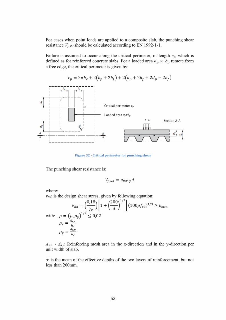
53

For cases when point loads are applied to a composite slab, the punching shear resistance Vp,Rd should be calculated according to EN 1992-1-1. Failure is assumed to occur along the critical perimeter, of length cp, which is defined as for reinforced concrete slabs. For a loaded area 𝑎𝑝 × 𝑏𝑝 remote from a free edge, the critical perimeter is given by:

𝑐𝑝 = 2𝜋ℎ𝑐 + 2�𝑏𝑝 + 2ℎ𝑓� + 2�𝑎𝑝 + 2ℎ𝑓 + 2𝑑𝑝 − 2ℎ𝑓�

Figure 32 - Critical perimeter for punching shear

The punching shear resistance is:

𝑉𝑝,𝑅𝑑 = 𝜐𝑅𝑑𝑐𝑝𝑑 where: νRd: is the design shear stress, given by following equation:

𝜈𝑅𝑑 = �0,18𝛾𝑐

� �1 + �200𝑑 �

1/2

� (100𝜌𝑓𝑐𝑘)1/3 ≥ 𝜐𝑚𝑖𝑛

with: 𝜌 = �𝜌𝑥𝜌𝑦�1/2 ≤ 0,02

𝜌𝑥 = 𝐴𝑠,𝑥ℎ𝑐

𝜌𝑦 = 𝐴𝑠,𝑦

ℎ𝑐

As,x - As,y: Reinforcing mesh area in the x-direction and in the y-direction per unit width of slab.

d: is the mean of the effective depths of the two layers of reinforcement, but not less than 200mm.

Critical perimeter cp

Loaded area apxbp

Section A-A

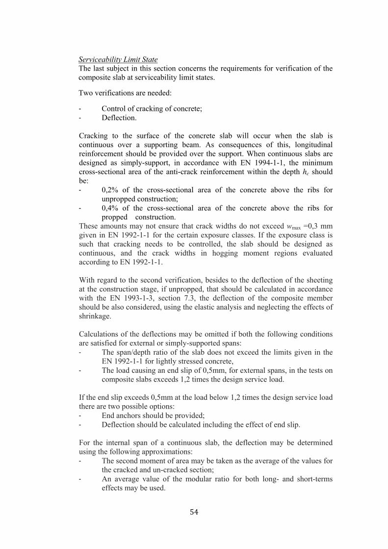
54

Serviceability Limit State The last subject in this section concerns the requirements for verification of the composite slab at serviceability limit states.

Two verifications are needed:

- Control of cracking of concrete; - Deflection. Cracking to the surface of the concrete slab will occur when the slab is continuous over a supporting beam. As consequences of this, longitudinal reinforcement should be provided over the support. When continuous slabs are designed as simply-support, in accordance with EN 1994-1-1, the minimum cross-sectional area of the anti-crack reinforcement within the depth hc should be: - 0,2% of the cross-sectional area of the concrete above the ribs for

unpropped construction; - 0,4% of the cross-sectional area of the concrete above the ribs for

propped construction. These amounts may not ensure that crack widths do not exceed wmax =0,3 mm given in EN 1992-1-1 for the certain exposure classes. If the exposure class is such that cracking needs to be controlled, the slab should be designed as continuous, and the crack widths in hogging moment regions evaluated according to EN 1992-1-1. With regard to the second verification, besides to the deflection of the sheeting at the construction stage, if unpropped, that should be calculated in accordance with the EN 1993-1-3, section 7.3, the deflection of the composite member should be also considered, using the elastic analysis and neglecting the effects of shrinkage. Calculations of the deflections may be omitted if both the following conditions are satisfied for external or simply-supported spans: - The span/depth ratio of the slab does not exceed the limits given in the

EN 1992-1-1 for lightly stressed concrete, - The load causing an end slip of 0,5mm, for external spans, in the tests on

composite slabs exceeds 1,2 times the design service load. If the end slip exceeds 0,5mm at the load below 1,2 times the design service load there are two possible options: - End anchors should be provided; - Deflection should be calculated including the effect of end slip. For the internal span of a continuous slab, the deflection may be determined using the following approximations: - The second moment of area may be taken as the average of the values for

the cracked and un-cracked section; - An average value of the modular ratio for both long- and short-terms

effects may be used.

55

In a cross-section where the concrete in tension is considered as cracked, the second moment of area Icc can be obtained from:

𝐼𝑐𝑐 =𝑏𝑥𝑐3

12𝑛+𝑏𝑥𝑐 �

𝑥𝑐2 �

2

𝑛+ 𝐴𝑝�𝑑𝑝 − 𝑥𝑐�

2 + 𝐼𝑝

with:

Ip: second moment of area of the profiled sheeting,

n: modulo ratio

xc: position of the elastic neutral axis to the upper side of the slab obtained by the following formula:

𝑥𝑐 = 𝑛𝐴𝑝𝑏 �1 + 2𝑏𝑑𝑝

𝑛𝐴𝑝− 1

In a section under sagging moment considering the concrete in tension as not cracked, the second moment of area Icu is given by:

𝐼𝑐𝑢 = 𝑏ℎ𝑐3

12𝑛+

𝑏ℎ𝑐�𝑥𝑢−ℎ𝑐2 �

2

𝑛+ 𝑏𝑚ℎ𝑝3

12𝑛+ 𝑏𝑚ℎ𝑝

𝑛�ℎ𝑡 − 𝑥𝑢 −

ℎ𝑝2�2

+ 𝐴𝑝�𝑑𝑝 − 𝑥𝑢�2 + 𝐼𝑝

where:

xu: is the position of the elastic neutral axis to the upper side of the slab, given by:

𝑥𝑢 = ∑𝐴𝑖𝑧𝑖 /∑𝐴𝑖

n: in this formula the modular ratio can be considered as the average value of the short and long term modular ratio:

𝑛 = 𝐸𝑎𝐸𝑐𝑚′

= 𝐸𝑎12�𝐸𝑐𝑚+

𝐸𝑐𝑚3 �

[4]

56

Testing of composite floor slabs All the tests are carried out in accordance with Annex B of EN 1994-1-1. Tests according to this section should be used for the determination of the factors m and k or τu,Rd to be used for the verification of the resistance to longitudinal shear.

From the load-deflection curves, obtained from the tests, the longitudinal shear behaviour is to be classified as brittle or ductile. Slab behaviour influences the determination of m and k factor.

The variable to be investigated include:

- Thickness; - Type of steel sheeting; - Steel grade; - Coating of the steel sheet; - Density and the quality of concrete; - Slab thickness; - Shear span length Ls.

For a complete investigation, it possible to reduce the number of tests avoid a prolonged and expensive research, if the results obtained may be used also for other values of variables as:

- The steel sheeting thickness t larger than tests; - The specified strength concrete fck not less than 0,8fcm, where fcm is the mean

value of the concrete strength in tests; - The yield strength of steel sheeting not less than 0,8fypm, where fypm is the mean

value of the yield strength in the test.

The test set-up foresees that: - The composite slab specimens are simply supported; - Two equal line loads are placed symmetrically at quarter span distance from the

centre line of supports; - A distance of 100mm is left between the centre line of the supports and the end

of the slab; - A distance of 100mm is left between the width of the bearing plates and the line

loads; - Neoprene pad with area not more than 100mm x b under the concentrated line

loads; - Single hydraulic jack is used to apply the load, which is distributed to the slab

trough a spreader beam system; - Mid-span and end-slip are measured by deflectometer and strain gauge; - Crack inducers are cast in place at the loading positions.

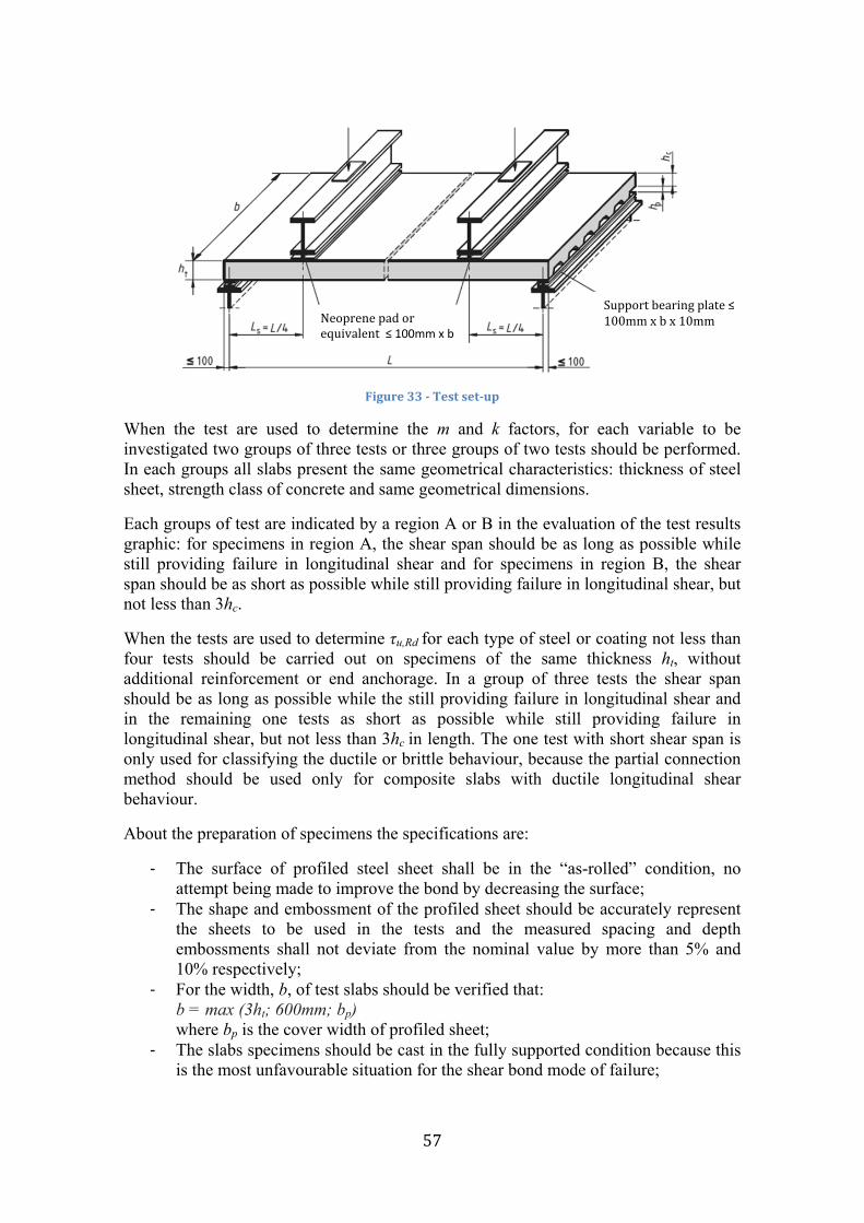
57

Figure 33 - Test set-up

When the test are used to determine the m and k factors, for each variable to be investigated two groups of three tests or three groups of two tests should be performed. In each groups all slabs present the same geometrical characteristics: thickness of steel sheet, strength class of concrete and same geometrical dimensions.

Each groups of test are indicated by a region A or B in the evaluation of the test results graphic: for specimens in region A, the shear span should be as long as possible while still providing failure in longitudinal shear and for specimens in region B, the shear span should be as short as possible while still providing failure in longitudinal shear, but not less than 3hc.

When the tests are used to determine τu,Rd for each type of steel or coating not less than four tests should be carried out on specimens of the same thickness ht, without additional reinforcement or end anchorage. In a group of three tests the shear span should be as long as possible while the still providing failure in longitudinal shear and in the remaining one tests as short as possible while still providing failure in longitudinal shear, but not less than 3hc in length. The one test with short shear span is only used for classifying the ductile or brittle behaviour, because the partial connection method should be used only for composite slabs with ductile longitudinal shear behaviour.

About the preparation of specimens the specifications are:

- The surface of profiled steel sheet shall be in the “as-rolled” condition, no attempt being made to improve the bond by decreasing the surface;

- The shape and embossment of the profiled sheet should be accurately represent the sheets to be used in the tests and the measured spacing and depth embossments shall not deviate from the nominal value by more than 5% and 10% respectively;

- For the width, b, of test slabs should be verified that: b = max (3ht; 600mm; bp) where bp is the cover width of profiled sheet;

- The slabs specimens should be cast in the fully supported condition because this is the most unfavourable situation for the shear bond mode of failure;

Neoprene pad or equivalent ≤ 100mm x b

Support bearing plate ≤ 100mm x b x 10mm

58

- The mesh reinforcement must be placed such that it acts in compression under the sagging moment;

- The concrete should be of the same mix and cured under the same conditions. For each group of slabs that will be tested within 48 hours, a minimum of four concrete specimens, for the determination of the cylinder or cube strength, should be prepared at time of casting the test slabs. The concrete strength fcm of each group should be taken as the mean value, when the deviation of each specimen from the mean value does not exceed 10%, otherwise when the deviation of the compressive strength from the mean value exceeds 10% the concrete strength should be taken as the maximum observed value;

- The tensile strength and yield strength of the profiled steel sheet should be obtained from coupon tests on specimens cut from each of the sheets used to form the test slabs.

The loading of slabs is of two types, dynamic or cyclic loading and static loading, where the slab is loaded to failure under an increasing load.

One of the test specimens in each group may be subject to just the static test without the cyclic loading in order to determine the level of the cyclic load for the other tests.

Initial test consists to load the slab under an imposed cyclic load, which varies between a lower value not greater than 0,2Wt and an upper value not less than 0,6Wt, where Wt is the measured failure load of the preliminary static test.

The loading should be applied for 5000 cycles in a time not less than 3 hours.

Subsequent test is a completion of the initial test, in fact the slab should be subjected to a static test where the imposed load is increased progressively, such the failure does not occur in less than 1 hour.

The failure load Wt is the maximum load imposed on the slab at failure plus the weight of the composite slab and spreader beams.

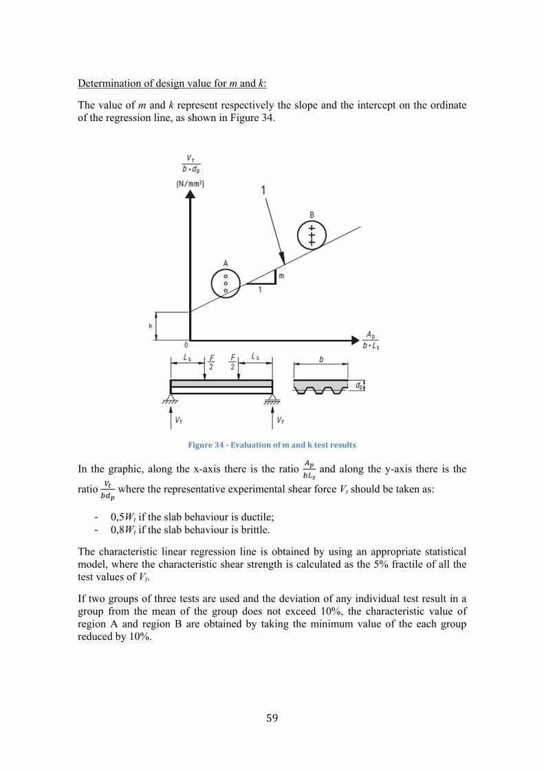
59

Determination of design value for m and k:

The value of m and k represent respectively the slope and the intercept on the ordinate of the regression line, as shown in Figure 34.

Figure 34 - Evaluation of m and k test results

In the graphic, along the x-axis there is the ratio 𝐴𝑝𝑏𝐿𝑠

and along the y-axis there is the

ratio 𝑉𝑡𝑏𝑑𝑝

where the representative experimental shear force Vt should be taken as:

- 0,5Wt if the slab behaviour is ductile; - 0,8Wt if the slab behaviour is brittle.

The characteristic linear regression line is obtained by using an appropriate statistical model, where the characteristic shear strength is calculated as the 5% fractile of all the test values of Vt.

If two groups of three tests are used and the deviation of any individual test result in a group from the mean of the group does not exceed 10%, the characteristic value of region A and region B are obtained by taking the minimum value of the each group reduced by 10%.

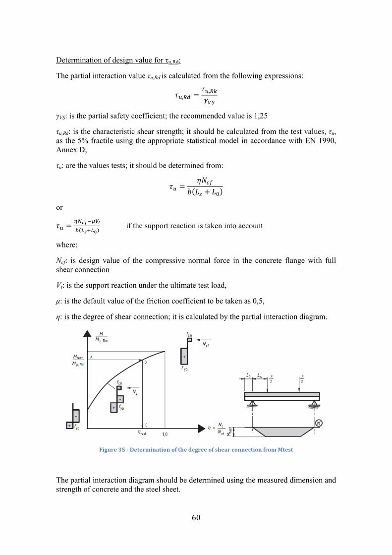
60

Determination of design value for τu,Rd:

The partial interaction value τu,Rd is calculated from the following expressions:

𝜏𝑢,𝑅𝑑 =𝜏𝑢,𝑅𝑘

𝛾𝑉𝑆

γVS: is the partial safety coefficient; the recommended value is 1,25

τu,Rk: is the characteristic shear strength; it should be calculated from the test values, τu, as the 5% fractile using the appropriate statistical model in accordance with EN 1990, Annex D;

τu: are the values tests; it should be determined from:

𝜏𝑢 =𝜂𝑁𝑐𝑓

𝑏(𝐿𝑠 + 𝐿0)

or

𝜏𝑢 = 𝜂𝑁𝑐𝑓−𝜇𝑉𝑡𝑏(𝐿𝑠+𝐿0)

if the support reaction is taken into account

where:

Ncf: is design value of the compressive normal force in the concrete flange with full shear connection

Vt: is the support reaction under the ultimate test load,

μ: is the default value of the friction coefficient to be taken as 0,5,

η: is the degree of shear connection; it is calculated by the partial interaction diagram.

Figure 35 - Determination of the degree of shear connection from Mtest

The partial interaction diagram should be determined using the measured dimension and strength of concrete and the steel sheet.

61

From the maximum applied loads, the bending moment M at the cross-section under the point load due to the applied load, dead weight of the slab and spreader beams should be determined with the following equation:

𝑀𝑡𝑒𝑠𝑡 = 𝑉𝑡 ×𝐿4

and when 𝜂 = 0, Mtest=Mpl,a

The path A -> B -> C gives a value η for each test.

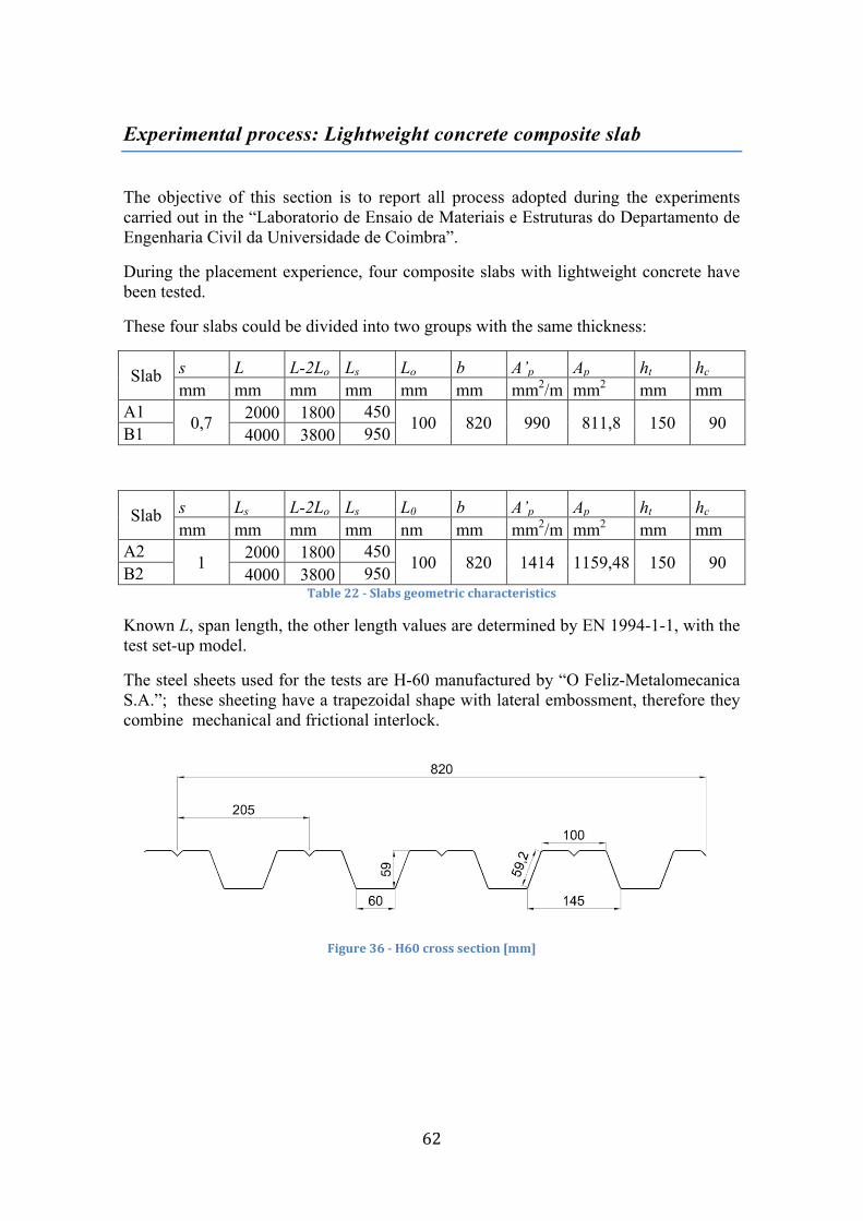
62

Experimental process: Lightweight concrete composite slab

The objective of this section is to report all process adopted during the experiments carried out in the “Laboratorio de Ensaio de Materiais e Estruturas do Departamento de Engenharia Civil da Universidade de Coimbra”.

During the placement experience, four composite slabs with lightweight concrete have been tested.

These four slabs could be divided into two groups with the same thickness:

Slab s L L-2Lo Ls Lo b A’p Ap ht hc mm mm mm mm mm mm mm2/m mm2 mm mm

A1 0,7 2000 1800 450 100 820 990 811,8 150 90 B1 4000 3800 950

Slab s Ls L-2Lo Ls L0 b A’p Ap ht hc mm mm mm mm nm mm mm2/m mm2 mm mm

A2 1 2000 1800 450 100 820 1414 1159,48 150 90 B2 4000 3800 950 Table 22 - Slabs geometric characteristics

Known L, span length, the other length values are determined by EN 1994-1-1, with the test set-up model.

The steel sheets used for the tests are H-60 manufactured by “O Feliz-Metalomecanica S.A.”; these sheeting have a trapezoidal shape with lateral embossment, therefore they combine mechanical and frictional interlock.

Figure 36 - H60 cross section [mm]

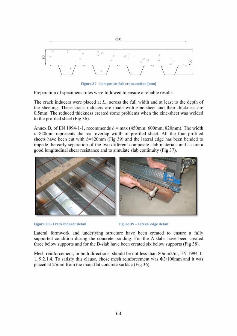
63

Figure 37 - Composite slab cross section [mm]

Preparation of specimens rules were followed to ensure a reliable results.

The crack inducers were placed at Ls, across the full width and at least to the depth of the sheeting. These crack inducers are made with zinc-sheet and their thickness are 0,5mm. The reduced thickness created some problems when the zinc-sheet was welded to the profiled sheet (Fig 36).

Annex B, of EN 1994-1-1, recommends b = max (450mm; 600mm; 820mm). The width b=820mm represents the real overlap width of profiled sheet. All the four profiled sheets have been cut with b=820mm (Fig 39) and the lateral edge has been bended to impede the early separation of the two different composite slab materials and assure a good longitudinal shear resistance and to simulate slab continuity (Fig 37).

Figure 38 – Crack inducer detail Figure 39 – Lateral edge detail

Lateral formwork and underlying structure have been created to ensure a fully supported condition during the concrete ponding. For the A-slabs have been created three below supports and for the B-slab have been created six below supports (Fig 38).

Mesh reinforcement, in both directions, should be not less than 80mm2/m, EN 1994-1-1, 9.2.1.4. To satisfy this clause, chose mesh reinforcement was Φ3/100mm and it was placed at 25mm from the main flat concrete surface (Fig 36).

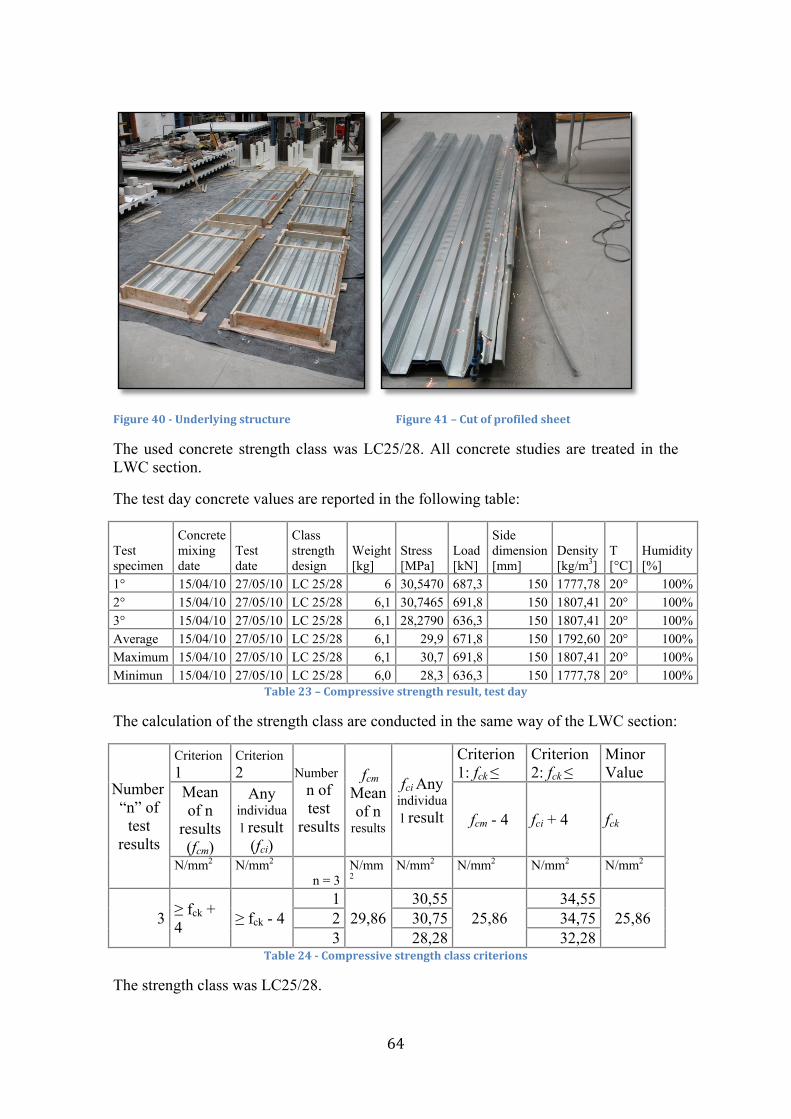
64

Figure 40 - Underlying structure Figure 41 – Cut of profiled sheet

The used concrete strength class was LC25/28. All concrete studies are treated in the LWC section.

The test day concrete values are reported in the following table:

Test specimen

Concrete mixing date

Test date

Class strength design

Weight [kg]

Stress [MPa]

Load [kN]

Side dimension [mm]

Density [kg/m3]

T [°C]

Humidity [%]

1° 15/04/10 27/05/10 LC 25/28 6 30,5470 687,3 150 1777,78 20° 100% 2° 15/04/10 27/05/10 LC 25/28 6,1 30,7465 691,8 150 1807,41 20° 100% 3° 15/04/10 27/05/10 LC 25/28 6,1 28,2790 636,3 150 1807,41 20° 100% Average 15/04/10 27/05/10 LC 25/28 6,1 29,9 671,8 150 1792,60 20° 100% Maximum 15/04/10 27/05/10 LC 25/28 6,1 30,7 691,8 150 1807,41 20° 100% Minimun 15/04/10 27/05/10 LC 25/28 6,0 28,3 636,3 150 1777,78 20° 100%

Table 23 – Compressive strength result, test day

The calculation of the strength class are conducted in the same way of the LWC section:

Number “n” of

test results

Criterion 1

Criterion 2 Number

n of test

results

fcm Mean of n

results

fci Any individual result

Criterion 1: fck ≤

Criterion 2: fck ≤

Minor Value

Mean of n

results (fcm)

Any individual result

(fci) fcm - 4 fci + 4 fck

N/mm2 N/mm2 n = 3

N/mm2

N/mm2 N/mm2 N/mm2 N/mm2

3 ≥ fck + 4 ≥ fck - 4

1 29,86

30,55 25,86

34,55 25,86 2 30,75 34,75

3 28,28 32,28 Table 24 - Compressive strength class criterions

The strength class was LC25/28.

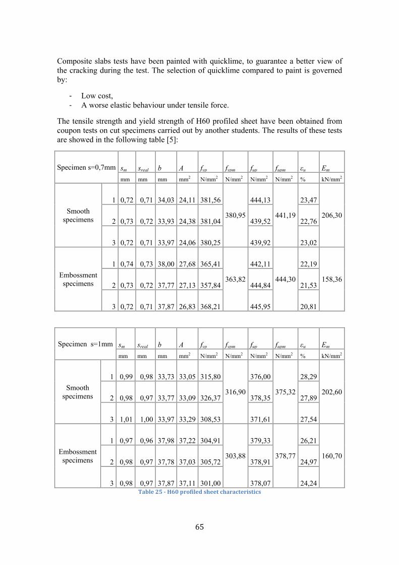
65

Composite slabs tests have been painted with quicklime, to guarantee a better view of the cracking during the test. The selection of quicklime compared to paint is governed by:

- Low cost, - A worse elastic behaviour under tensile force.

The tensile strength and yield strength of H60 profiled sheet have been obtained from coupon tests on cut specimens carried out by another students. The results of these tests are showed in the following table [5]:

Specimen s=0,7mm sm sreal b A fyp fypm fup fupm εu Em mm mm mm mm2 N/mm2 N/mm2 N/mm2 N/mm2 % kN/mm2

Smooth specimens

1 0,72 0,71 34,03 24,11 381,56

380,95

444,13

441,19

23,47

206,30 2 0,73 0,72 33,93 24,38 381,04 439,52 22,76

3 0,72 0,71 33,97 24,06 380,25 439,92 23,02

Embossment specimens

1 0,74 0,73 38,00 27,68 365,41

363,82

442,11

444,30

22,19

158,36 2 0,73 0,72 37,77 27,13 357,84 444,84 21,53

3 0,72 0,71 37,87 26,83 368,21 445,95 20,81

Specimen s=1mm sm sreal b A fyp fypm fup fupm εu Em mm mm mm mm2 N/mm2 N/mm2 N/mm2 N/mm2 % kN/mm2

Smooth specimens

1 0,99 0,98 33,73 33,05 315,80

316,90

376,00

375,32

28,29

202,60 2 0,98 0,97 33,77 33,09 326,37 378,35 27,89

3 1,01 1,00 33,97 33,29 308,53 371,61 27,54

Embossment specimens

1 0,97 0,96 37,98 37,22 304,91

303,88

379,33

378,77

26,21

160,70 2 0,98 0,97 37,78 37,03 305,72 378,91 24,97

3 0,98 0,97 37,87 37,11 301,00 378,07 24,24 Table 25 - H60 profiled sheet characteristics

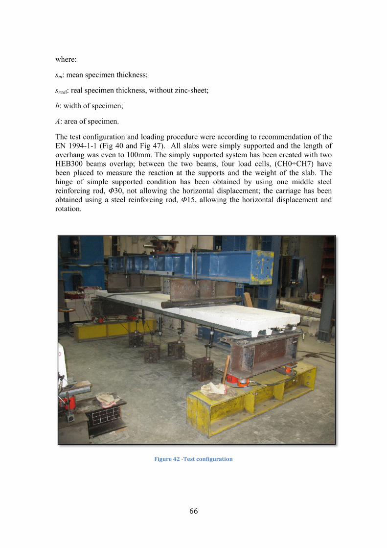
66

where:

sm: mean specimen thickness;

sreal: real specimen thickness, without zinc-sheet;

b: width of specimen;

A: area of specimen.

The test configuration and loading procedure were according to recommendation of the EN 1994-1-1 (Fig 40 and Fig 47). All slabs were simply supported and the length of overhang was even to 100mm. The simply supported system has been created with two HEB300 beams overlap; between the two beams, four load cells, (CH0÷CH7) have been placed to measure the reaction at the supports and the weight of the slab. The hinge of simple supported condition has been obtained by using one middle steel reinforcing rod, Φ30, not allowing the horizontal displacement; the carriage has been obtained using a steel reinforcing rod, Φ15, allowing the horizontal displacement and rotation.

Figure 42 -Test configuration

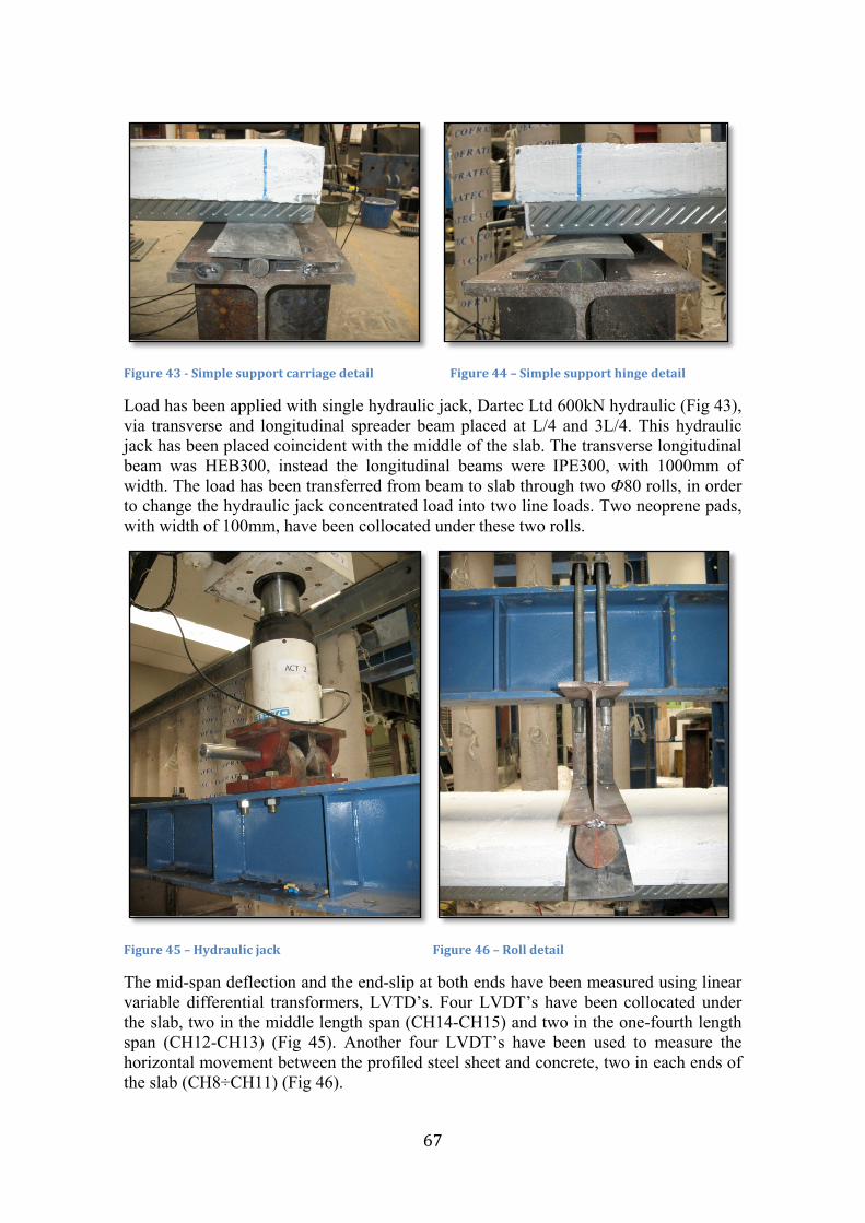
67

Figure 43 - Simple support carriage detail Figure 44 – Simple support hinge detail

Load has been applied with single hydraulic jack, Dartec Ltd 600kN hydraulic (Fig 43), via transverse and longitudinal spreader beam placed at L/4 and 3L/4. This hydraulic jack has been placed coincident with the middle of the slab. The transverse longitudinal beam was HEB300, instead the longitudinal beams were IPE300, with 1000mm of width. The load has been transferred from beam to slab through two Φ80 rolls, in order to change the hydraulic jack concentrated load into two line loads. Two neoprene pads, with width of 100mm, have been collocated under these two rolls.

Figure 45 – Hydraulic jack Figure 46 – Roll detail

The mid-span deflection and the end-slip at both ends have been measured using linear variable differential transformers, LVTD’s. Four LVDT’s have been collocated under the slab, two in the middle length span (CH14-CH15) and two in the one-fourth length span (CH12-CH13) (Fig 45). Another four LVDT’s have been used to measure the horizontal movement between the profiled steel sheet and concrete, two in each ends of the slab (CH8÷CH11) (Fig 46).

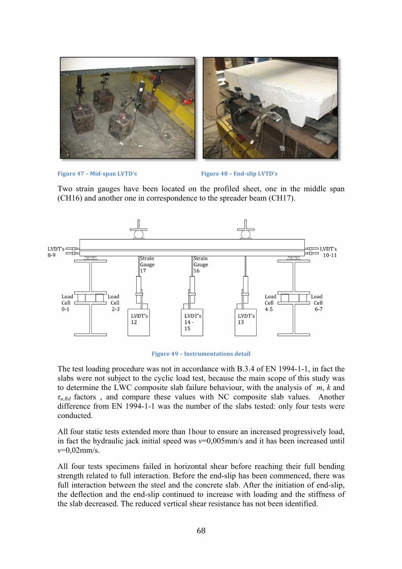
68

Figure 47 – Mid-span LVTD’s Figure 48 – End-slip LVTD’s

Two strain gauges have been located on the profiled sheet, one in the middle span (CH16) and another one in correspondence to the spreader beam (CH17).

Figure 49 – Instrumentations detail

The test loading procedure was not in accordance with B.3.4 of EN 1994-1-1, in fact the slabs were not subject to the cyclic load test, because the main scope of this study was to determine the LWC composite slab failure behaviour, with the analysis of m, k and τu,Rd factors , and compare these values with NC composite slab values. Another difference from EN 1994-1-1 was the number of the slabs tested: only four tests were conducted.

All four static tests extended more than 1hour to ensure an increased progressively load, in fact the hydraulic jack initial speed was v=0,005mm/s and it has been increased until v=0,02mm/s.

All four tests specimens failed in horizontal shear before reaching their full bending strength related to full interaction. Before the end-slip has been commenced, there was full interaction between the steel and the concrete slab. After the initiation of end-slip, the deflection and the end-slip continued to increase with loading and the stiffness of the slab decreased. The reduced vertical shear resistance has not been identified.

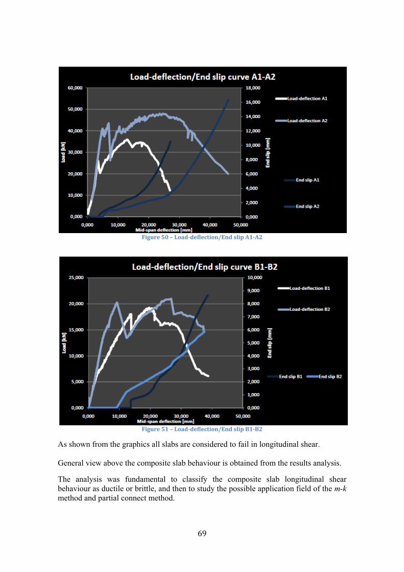
69

Figure 50 – Load-deflection/End slip A1-A2

Figure 51 – Load-deflection/End slip B1-B2

As shown from the graphics all slabs are considered to fail in longitudinal shear. General view above the composite slab behaviour is obtained from the results analysis.

The analysis was fundamental to classify the composite slab longitudinal shear behaviour as ductile or brittle, and then to study the possible application field of the m-k method and partial connect method.

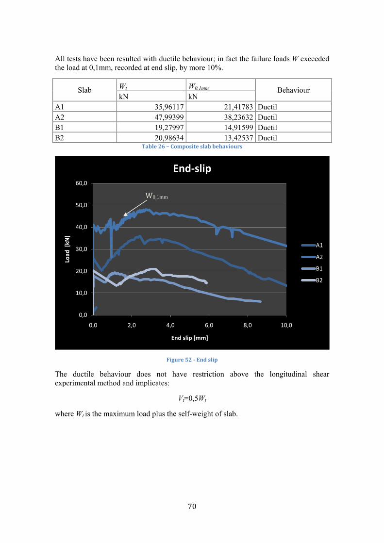
70

All tests have been resulted with ductile behaviour; in fact the failure loads W exceeded the load at 0,1mm, recorded at end slip, by more 10%.

Slab Wt W0,1mm Behaviour kN kN

A1 35,96117 21,41783 Ductil A2 47,99399 38,23632 Ductil B1 19,27997 14,91599 Ductil B2 20,98634 13,42537 Ductil

Table 26 – Composite slab behaviours

Figure 52 - End slip

The ductile behaviour does not have restriction above the longitudinal shear experimental method and implicates:

Vt=0,5Wt

where Wt is the maximum load plus the self-weight of slab.

0,0

10,0

20,0

30,0

40,0

50,0

60,0

0,0 2,0 4,0 6,0 8,0 10,0

Load

[kN

]

End slip [mm]

End-slip

A1

A2

B1

B2

W0,1mm

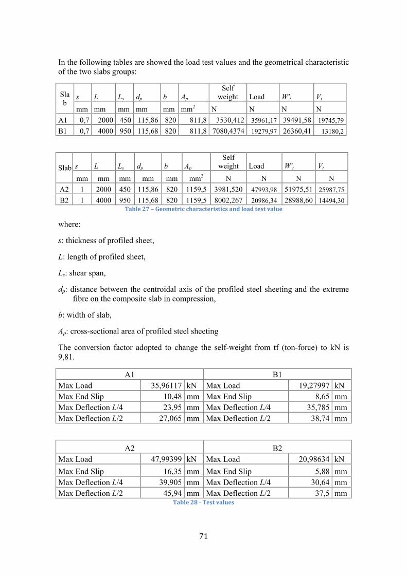
71

In the following tables are showed the load test values and the geometrical characteristic of the two slabs groups:

Slab

s L Ls dp b Ap Self

weight Load W't Vt mm mm mm mm mm mm2 N N N N

A1 0,7 2000 450 115,86 820 811,8 3530,412 35961,17 39491,58 19745,79 B1 0,7 4000 950 115,68 820 811,8 7080,4374 19279,97 26360,41 13180,2

Slab s L Ls dp b Ap Self

weight Load W't Vt mm mm mm mm mm mm2 N N N N

A2 1 2000 450 115,86 820 1159,5 3981,520 47993,98 51975,51 25987,75 B2 1 4000 950 115,68 820 1159,5 8002,267 20986,34 28988,60 14494,30

Table 27 – Geometric characteristics and load test value

where:

s: thickness of profiled sheet,

L: length of profiled sheet,

Ls: shear span,

dp: distance between the centroidal axis of the profiled steel sheeting and the extreme fibre on the composite slab in compression,

b: width of slab,

Ap: cross-sectional area of profiled steel sheeting

The conversion factor adopted to change the self-weight from tf (ton-force) to kN is 9,81.

A1 B1 Max Load 35,96117 kN Max Load 19,27997 kN Max End Slip 10,48 mm Max End Slip 8,65 mm Max Deflection L/4 23,95 mm Max Deflection L/4 35,785 mm Max Deflection L/2 27,065 mm Max Deflection L/2 38,74 mm

A2 B2 Max Load 47,99399 kN Max Load 20,98634 kN Max End Slip 16,35 mm Max End Slip 5,88 mm Max Deflection L/4 39,905 mm Max Deflection L/4 30,64 mm Max Deflection L/2 45,94 mm Max Deflection L/2 37,5 mm

Table 28 - Test values

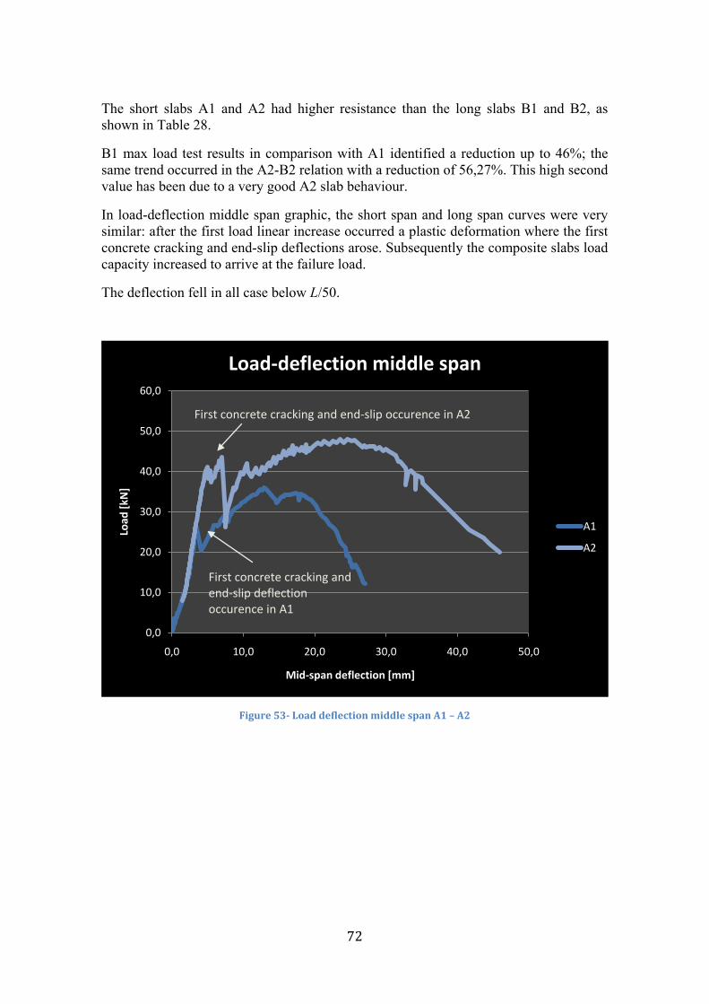
72

The short slabs A1 and A2 had higher resistance than the long slabs B1 and B2, as shown in Table 28.

B1 max load test results in comparison with A1 identified a reduction up to 46%; the same trend occurred in the A2-B2 relation with a reduction of 56,27%. This high second value has been due to a very good A2 slab behaviour.

In load-deflection middle span graphic, the short span and long span curves were very similar: after the first load linear increase occurred a plastic deformation where the first concrete cracking and end-slip deflections arose. Subsequently the composite slabs load capacity increased to arrive at the failure load.

The deflection fell in all case below L/50.

Figure 53- Load deflection middle span A1 – A2

0,0

10,0

20,0

30,0

40,0

50,0

60,0

0,0 10,0 20,0 30,0 40,0 50,0

Load

[kN

]

Mid-span deflection [mm]

Load-deflection middle span

A1

A2

First concrete cracking and end-slip occurence in A2

First concrete cracking and end-slip deflection occurence in A1

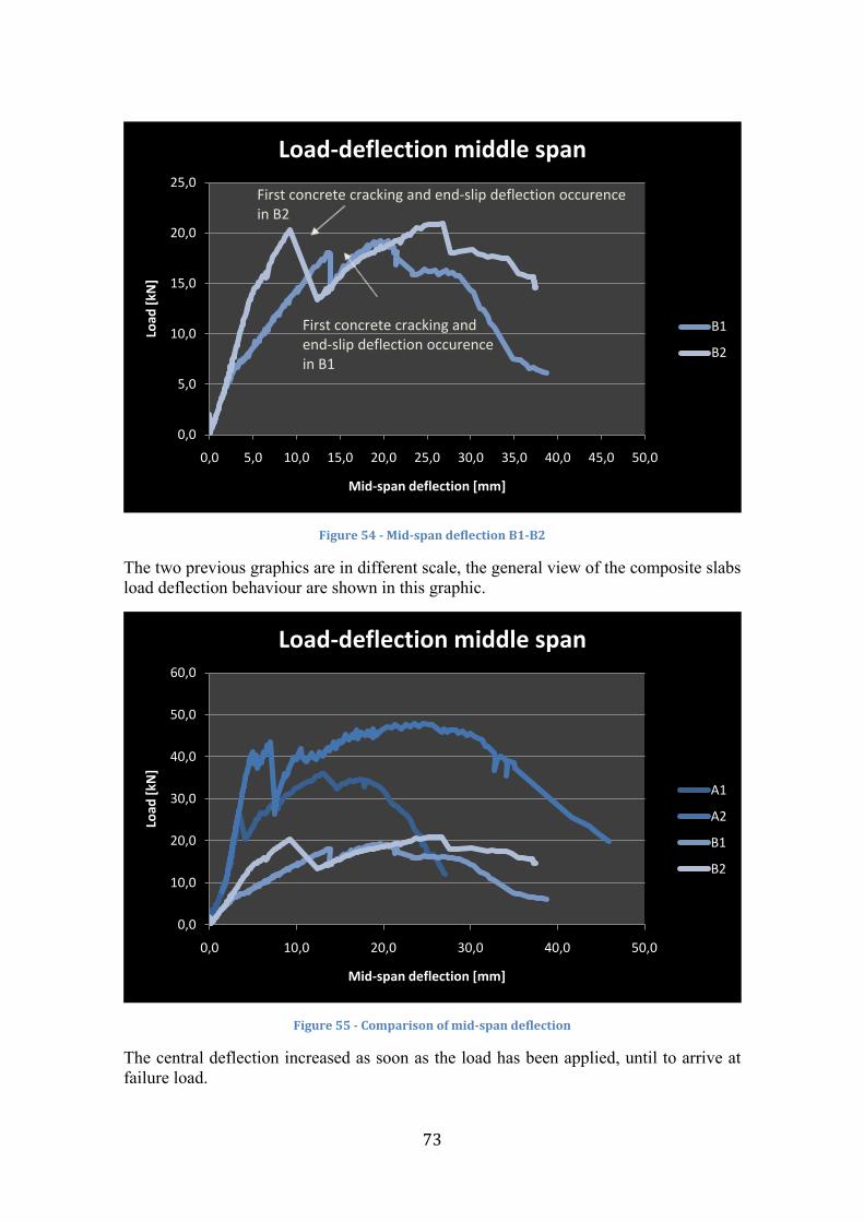
73

Figure 54 - Mid-span deflection B1-B2

The two previous graphics are in different scale, the general view of the composite slabs load deflection behaviour are shown in this graphic.

Figure 55 - Comparison of mid-span deflection

The central deflection increased as soon as the load has been applied, until to arrive at failure load.

0,0

5,0

10,0

15,0

20,0

25,0

0,0 5,0 10,0 15,0 20,0 25,0 30,0 35,0 40,0 45,0 50,0

Load

[kN

]

Mid-span deflection [mm]

Load-deflection middle span

B1

B2

First concrete cracking and end-slip deflection occurence in B2

First concrete cracking and end-slip deflection occurence in B1

0,0

10,0

20,0

30,0

40,0

50,0

60,0

0,0 10,0 20,0 30,0 40,0 50,0

Load

[kN

]

Mid-span deflection [mm]

Load-deflection middle span

A1

A2

B1

B2

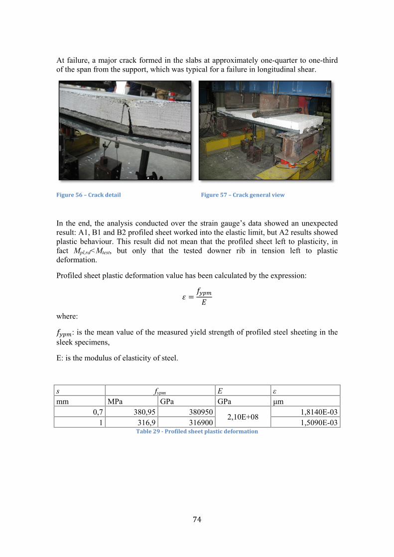
74

At failure, a major crack formed in the slabs at approximately one-quarter to one-third of the span from the support, which was typical for a failure in longitudinal shear.

Figure 56 – Crack detail Figure 57 – Crack general view

In the end, the analysis conducted over the strain gauge’s data showed an unexpected result: A1, B1 and B2 profiled sheet worked into the elastic limit, but A2 results showed plastic behaviour. This result did not mean that the profiled sheet left to plasticity, in fact Mpl,rd<Mtest, but only that the tested downer rib in tension left to plastic deformation.

Profiled sheet plastic deformation value has been calculated by the expression:

𝜀 =𝑓𝑦𝑝𝑚𝐸

where:

𝑓𝑦𝑝𝑚: is the mean value of the measured yield strength of profiled steel sheeting in the sleek specimens,

E: is the modulus of elasticity of steel.

s fypm E ε mm MPa GPa GPa μm

0,7 380,95 380950 2,10E+08 1,8140E-03 1 316,9 316900 1,5090E-03

Table 29 - Profiled sheet plastic deformation

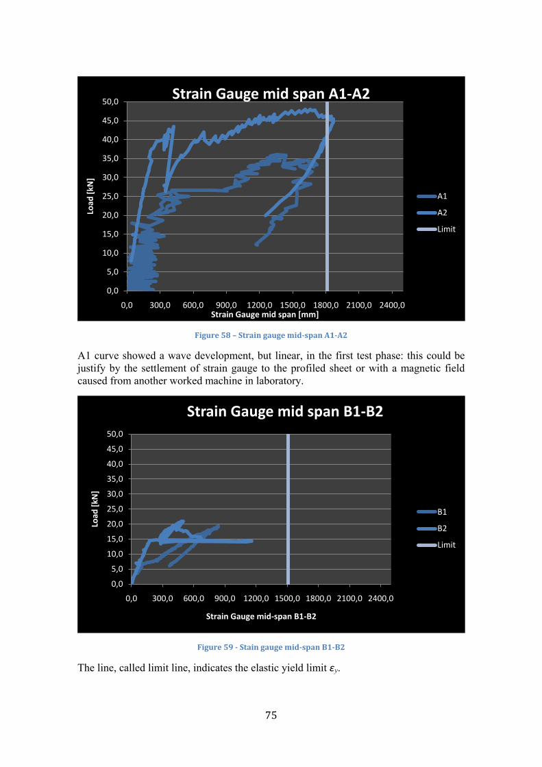
75

Figure 58 – Strain gauge mid-span A1-A2

A1 curve showed a wave development, but linear, in the first test phase: this could be justify by the settlement of strain gauge to the profiled sheet or with a magnetic field caused from another worked machine in laboratory.

Figure 59 - Stain gauge mid-span B1-B2

The line, called limit line, indicates the elastic yield limit εy.

0,0

5,0

10,0

15,0

20,0

25,0

30,0

35,0

40,0

45,0

50,0

0,0 300,0 600,0 900,0 1200,0 1500,0 1800,0 2100,0 2400,0

Load

[kN

]

Strain Gauge mid span [mm]

Strain Gauge mid span A1-A2

A1

A2

Limit

0,0

5,0

10,0

15,0

20,0

25,0

30,0

35,0

40,0

45,0

50,0

0,0 300,0 600,0 900,0 1200,0 1500,0 1800,0 2100,0 2400,0

Load

[kN

]

Strain Gauge mid-span B1-B2

Strain Gauge mid span B1-B2

B1

B2

Limit

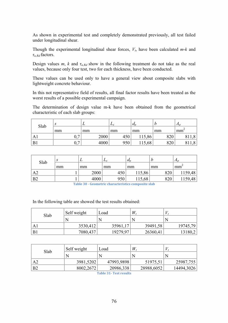
76

As shown in experimental test and completely demonstrated previously, all test failed under longitudinal shear.

Though the experimental longitudinal shear forces, Vt, have been calculated m-k and τu,Rd factors.

Design values m, k and τu,Rd show in the following treatment do not take as the real values, because only four test, two for each thickness, have been conducted.

These values can be used only to have a general view about composite slabs with lightweight concrete behaviour.

In this not representative field of results, all final factor results have been treated as the worst results of a possible experimental campaign.

The determination of design value m-k have been obtained from the geometrical characteristic of each slab groups:

Slab s L Ls dp b Ap mm mm mm mm mm mm2

A1 0,7 2000 450 115,86 820 811,8 B1 0,7 4000 950 115,68 820 811,8

Slab s L Ls dp b Ap mm mm mm mm mm mm2

A2 1 2000 450 115,86 820 1159,48 B2 1 4000 950 115,68 820 1159,48

Table 30 - Geometric characteristics composite slab

In the following table are showed the test results obtained:

Slab Self weight Load Wt Vt N N N N

A1 3530,412 35961,17 39491,58 19745,79 B1 7080,437 19279,97 26360,41 13180,2

Slab Self weight Load Wt Vt N N N N

A2 3981,5202 47993,9898 51975,51 25987,755 B2 8002,2672 20986,338 28988,6052 14494,3026

Table 31- Test results

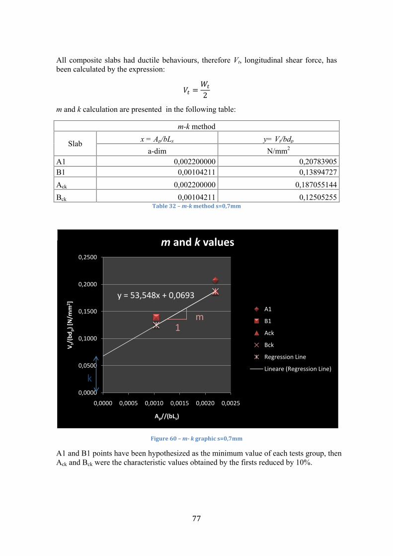
77

All composite slabs had ductile behaviours, therefore Vt, longitudinal shear force, has been calculated by the expression:

𝑉𝑡 =𝑊𝑡

2

m and k calculation are presented in the following table:

m-k method

Slab x = Ap/bLs y= Vt/bdp a-dim N/mm2

A1 0,002200000 0,20783905 B1 0,00104211 0,13894727 Ack 0,002200000 0,187055144 Bck 0,00104211 0,12505255

Table 32 – m-k method s=0,7mm

Figure 60 – m- k graphic s=0,7mm

A1 and B1 points have been hypothesized as the minimum value of each tests group, then Ack and Bck were the characteristic values obtained by the firsts reduced by 10%.

y = 53,548x + 0,0693

0,0000

0,0500

0,1000

0,1500

0,2000

0,2500

0,0000 0,0005 0,0010 0,0015 0,0020 0,0025

V t/(b

d p) [N

/mm

2 ]

Ap//(bLs)

m and k values

A1

B1

Ack

Bck

Regression Line

Lineare (Regression Line)

k

m1

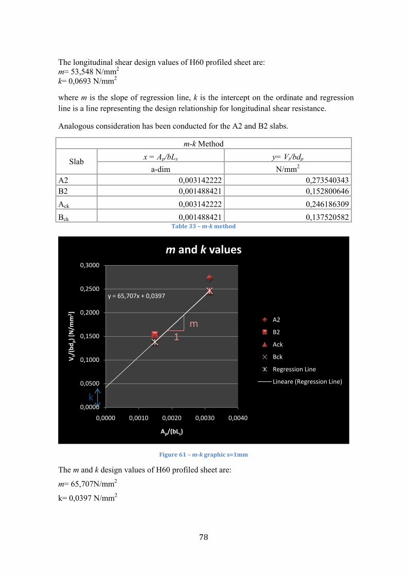
78

The longitudinal shear design values of H60 profiled sheet are: m= 53,548 N/mm2 k= 0,0693 N/mm2

where m is the slope of regression line, k is the intercept on the ordinate and regression line is a line representing the design relationship for longitudinal shear resistance.

Analogous consideration has been conducted for the A2 and B2 slabs.

m-k Method

Slab x = Ap/bLs y= Vt/bdp a-dim N/mm2

A2 0,003142222 0,273540343 B2 0,001488421 0,152800646 Ack 0,003142222 0,246186309 Bck 0,001488421 0,137520582

Table 33 – m-k method

Figure 61 – m-k graphic s=1mm

The m and k design values of H60 profiled sheet are:

m= 65,707N/mm2

k= 0,0397 N/mm2

y = 65,707x + 0,0397

0,0000

0,0500

0,1000

0,1500

0,2000

0,2500

0,3000

0,0000 0,0010 0,0020 0,0030 0,0040

V t/(b

d p) [N

/mm

2 ]

Ap/(bLs)

m and k values

A2

B2

Ack

Bck

Regression Line

Lineare (Regression Line)

k

m1

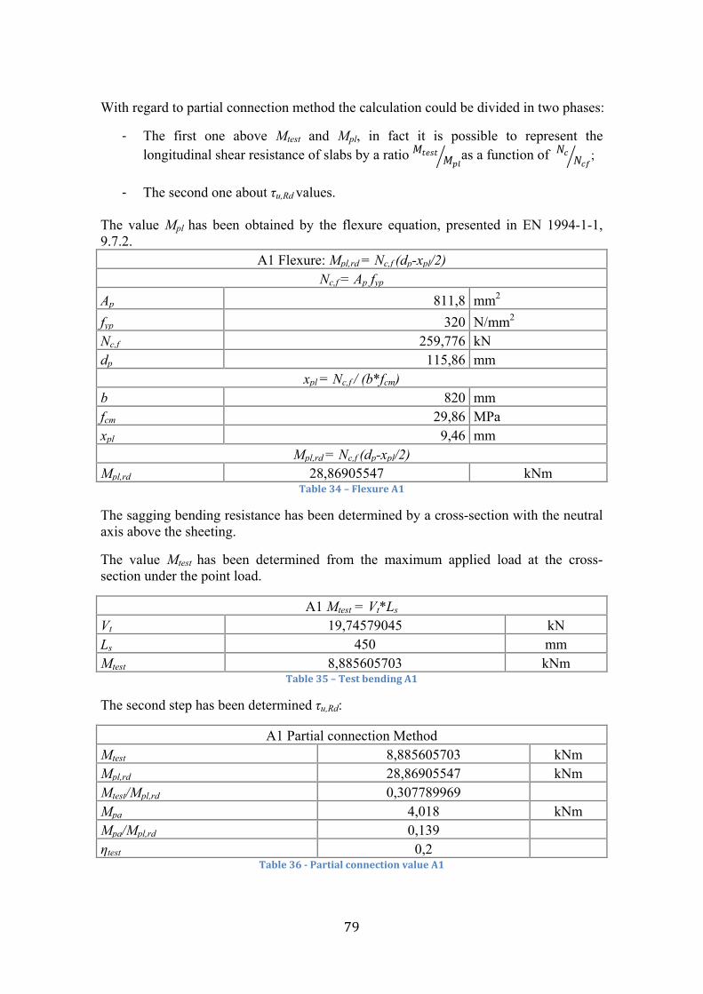
79

With regard to partial connection method the calculation could be divided in two phases:

- The first one above Mtest and Mpl, in fact it is possible to represent the longitudinal shear resistance of slabs by a ratio 𝑀𝑡𝑒𝑠𝑡

𝑀𝑝𝑙� as a function of 𝑁𝑐 𝑁𝑐𝑓� ;

- The second one about τu,Rd values.

The value Mpl has been obtained by the flexure equation, presented in EN 1994-1-1, 9.7.2.

A1 Flexure: Mpl,rd = Nc,f (dp-xpl/2) Nc,f = Ap fyp

Ap 811,8 mm2 fyp 320 N/mm2 Nc,f 259,776 kN dp 115,86 mm

xpl = Nc,f / (b*fcm) b 820 mm fcm 29,86 MPa xpl 9,46 mm

Mpl,rd = Nc,f (dp-xpl/2) Mpl,rd 28,86905547 kNm

Table 34 – Flexure A1

The sagging bending resistance has been determined by a cross-section with the neutral axis above the sheeting.

The value Mtest has been determined from the maximum applied load at the cross-section under the point load.

A1 Mtest = Vt*Ls Vt 19,74579045 kN Ls 450 mm Mtest 8,885605703 kNm

Table 35 – Test bending A1

The second step has been determined τu,Rd:

A1 Partial connection Method Mtest 8,885605703 kNm Mpl,rd 28,86905547 kNm Mtest/Mpl,rd 0,307789969 Mpa 4,018 kNm Mpa/Mpl,rd 0,139 ηtest 0,2

Table 36 - Partial connection value A1

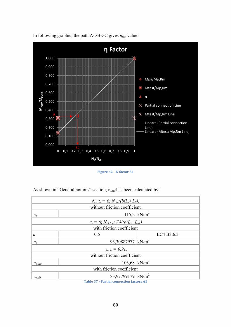
80

In following graphic, the path A->B->C gives ηtest value:

Figure 62 – N factor A1

As shown in “General notions” section, τu,Rd has been calculated by:

A1 τu = (η Ncf)/(b(Ls+L0)) without friction coefficient

τu 115,2 kN/m2 τu = (η Ncf - μ Vt)/(b(Ls+L0))

with friction coefficient μ 0,5 EC4 B3.6.3 τu 93,30887977 kN/m2

τu,Rk = 0,9τu without friction coefficient

τu,Rk 103,68 kN/m2 with friction coefficient

τu,Rk 83,97799179 kN/m2 Table 37 - Partial connection factors A1

0,000

0,100

0,200

0,300

0,400

0,500

0,600

0,700

0,800

0,900

1,000

0 0,1 0,2 0,3 0,4 0,5 0,6 0,7 0,8 0,9 1

Mt es

t/M

pl,R

d

Nc/Ncf

η Factor

Mpa/Mp,Rm

Mtest/Mp,Rm

n

Partial connection Line

Mtest/Mp,Rm Line

Lineare (Partial connection Line)Lineare (Mtest/Mp,Rm Line)

B A

C

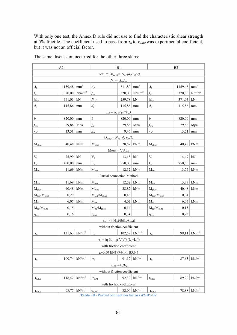
81

With only one test, the Annex D rule did not use to find the characteristic shear strength at 5% fractile. The coefficient used to pass from τu to τu,Rd was experimental coefficient, but it was not an official factor.

The same discussion occurred for the other three slabs:

A2 B1 B2

Flexure: Mpl,rd = Nc,f (dp-xpl/2)

Nc,f = Ap fyp

Ap 1159,48 mm2 Ap 811,80 mm2 Ap 1159,48 mm2

fyp 320,00 N/mm2 fyp 320,00 N/mm2 fyp 320,00 N/mm2

Nc,f 371,03 kN Nc,f 259,78 kN Nc,f 371,03 kN

dp 115,86 mm dp 115,86 mm dp 115,86 mm

xpl = Nc,f / (b*fcm)

b 820,00 mm b 820,00 mm b 820,00 mm

fcm 29,86 Mpa fcm 29,86 Mpa fcm 29,86 Mpa

xpl 13,51 mm xpl 9,46 mm xpl 13,51 mm

Mpl,rd = Nc,f (dp-xpl/2)

Mpl,rd 40,48 kNm Mpl,rd 28,87 kNm Mpl,rd 40,48 kNm

Mtest = Vt*Ls

Vt 25,99 kN Vt 13,18 kN Vt 14,49 kN

Ls 450,00 mm Ls 950,00 mm Ls 950,00 mm

Mtest 11,69 kNm Mtest 12,52 kNm Mtest 13,77 kNm

Partial connection Method

Mtest 11,69 kNm Mtest 12,52 kNm Mtest 13,77 kNm

Mpl,rd 40,48 kNm Mpl,rd 28,87 kNm Mpl,rd 40,48 kNm

Mtest/Mpl,rd 0,29 Mtest/Mpl,rd 0,43 Mtest/Mpl,rd 0,34

Mpa 6,07 kNm Mpa 4,02 kNm Mpa 6,07 kNm

Mpa/Mpl,rd 0,15 Mpa/Mpl,rd 0,14 Mpa/Mpl,rd 0,15

ηtest 0,16 ηtest 0,34 ηtest 0,23

τu = (η Ncf)/(b(Ls+L0))

without friction coefficient

τu 131,63 kN/m2 τu 102,58 kN/m2 τu 99,11 kN/m2

τu = (η Ncf - μ Vt)/(b(Ls+L0))

with friction coefficient

μ=0,50 EN1994-1-1 B3.6.3

τu 109,74 kN/m2 τu 91,12 kN/m2 τu 87,65 kN/m2

τu,Rk = 0,9τu

without friction coefficient

τu,Rk 118,47 kN/m2 τu,Rk 92,32 kN/m2 τu,Rk 89,20 kN/m2

with friction coefficient

τu,Rk 98,77 kN/m2 τu,Rk 82,00 kN/m2 τu,Rk 78,88 kN/m2 Table 38 - Partial connection factors A2-B1-B2

82

The calculations showed Mtest<Mpl,Rd; this meant that the composite slabs did not failure in the first critical section and it was another confirmation that A2 composite slab did not leave at plastic behaviour.

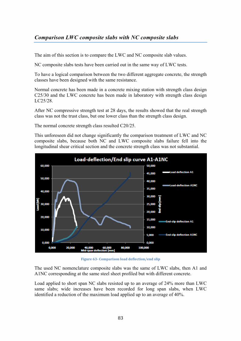
83

Comparison LWC composite slabs with NC composite slabs

The aim of this section is to compare the LWC and NC composite slab values.

NC composite slabs tests have been carried out in the same way of LWC tests.

To have a logical comparison between the two different aggregate concrete, the strength classes have been designed with the same resistance.

Normal concrete has been made in a concrete mixing station with strength class design C25/30 and the LWC concrete has been made in laboratory with strength class design LC25/28.

After NC compressive strength test at 28 days, the results showed that the real strength class was not the trust class, but one lower class than the strength class design.

The normal concrete strength class resulted C20/25.

This unforeseen did not change significantly the comparison treatment of LWC and NC composite slabs, because both NC and LWC composite slabs failure fell into the longitudinal shear critical section and the concrete strength class was not substantial.

Figure 63- Comparison load deflection/end slip

The used NC nomenclature composite slabs was the same of LWC slabs, then A1 and A1NC corresponding at the same steel sheet profiled but with different concrete.

Load applied to short span NC slabs resisted up to an average of 24% more than LWC same slabs; wide increases have been recorded for long span slabs, when LWC identified a reduction of the maximum load applied up to an average of 40%.

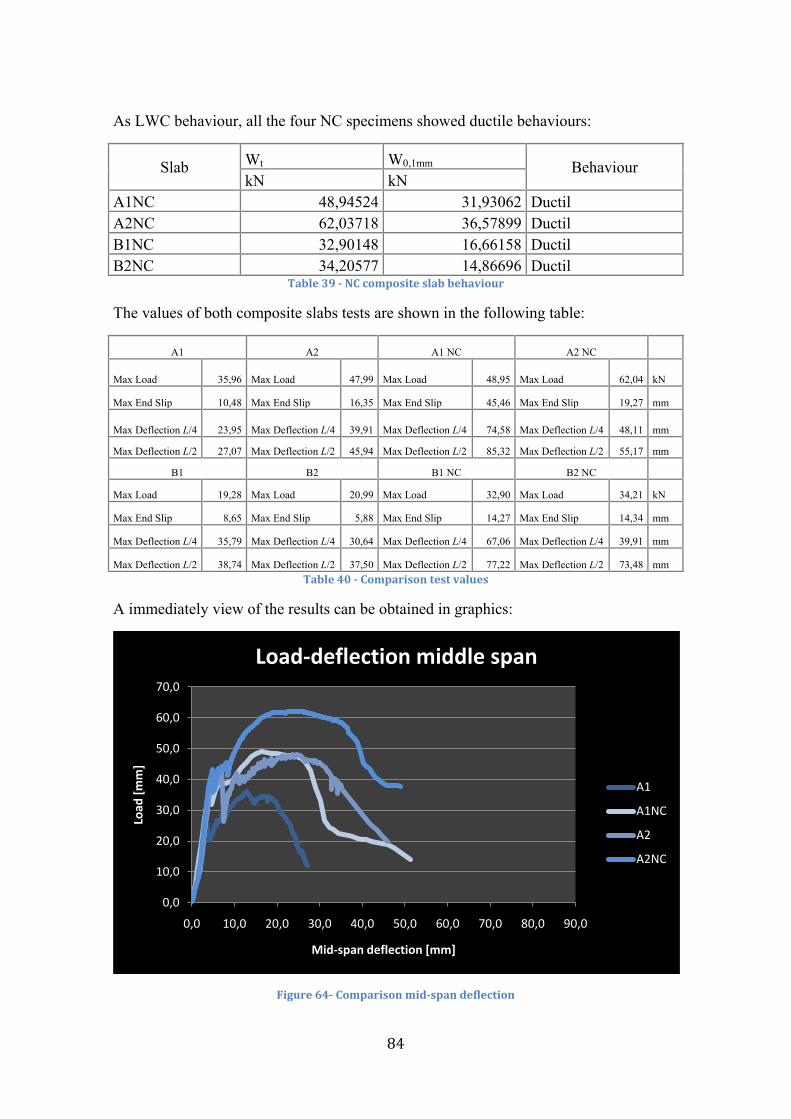
84

As LWC behaviour, all the four NC specimens showed ductile behaviours:

Slab Wt W0,1mm Behaviour kN kN

A1NC 48,94524 31,93062 Ductil A2NC 62,03718 36,57899 Ductil B1NC 32,90148 16,66158 Ductil B2NC 34,20577 14,86696 Ductil

Table 39 - NC composite slab behaviour

The values of both composite slabs tests are shown in the following table:

A1 A2 A1 NC A2 NC

Max Load 35,96 Max Load 47,99 Max Load 48,95 Max Load 62,04 kN

Max End Slip 10,48 Max End Slip 16,35 Max End Slip 45,46 Max End Slip 19,27 mm

Max Deflection L/4 23,95 Max Deflection L/4 39,91 Max Deflection L/4 74,58 Max Deflection L/4 48,11 mm

Max Deflection L/2 27,07 Max Deflection L/2 45,94 Max Deflection L/2 85,32 Max Deflection L/2 55,17 mm

B1 B2 B1 NC B2 NC

Max Load 19,28 Max Load 20,99 Max Load 32,90 Max Load 34,21 kN

Max End Slip 8,65 Max End Slip 5,88 Max End Slip 14,27 Max End Slip 14,34 mm

Max Deflection L/4 35,79 Max Deflection L/4 30,64 Max Deflection L/4 67,06 Max Deflection L/4 39,91 mm

Max Deflection L/2 38,74 Max Deflection L/2 37,50 Max Deflection L/2 77,22 Max Deflection L/2 73,48 mm Table 40 - Comparison test values

A immediately view of the results can be obtained in graphics:

Figure 64- Comparison mid-span deflection

0,0

10,0

20,0

30,0

40,0

50,0

60,0

70,0

0,0 10,0 20,0 30,0 40,0 50,0 60,0 70,0 80,0 90,0

Load

[mm

]

Mid-span deflection [mm]

Load-deflection middle span

A1

A1NC

A2

A2NC

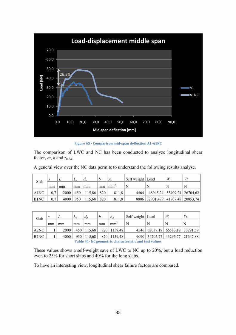
85

Figure 65 - Comparison mid-span deflection A1-A1NC

The comparison of LWC and NC has been conducted to analyze longitudinal shear factor, m, k and τu,Rd.

A general view over the NC data permits to understand the following results analyse.

Slab s L Ls dp b Ap Self weight Load Wt Vt

mm mm mm mm mm mm2 N N N N A1NC 0,7 2000 450 115,86 820 811,8 4464 48945,24 53409,24 26704,62 B1NC 0,7 4000 950 115,68 820 811,8 8806 32901,479 41707,48 20853,74

Slab s L Ls dp b Ap Self weight Load Wt Vt

mm mm mm mm mm mm2 N N N N A2NC 1 2000 450 115,68 820 1159,48 4546 62037,18 66583,18 33291,59 B2NC 1 4000 950 115,68 820 1159,48 9090 34205,77 43295,77 21647,88

Table 41- NC geometric characteristic and test values

These values shows a self-weight save of LWC to NC up to 20%, but a load reduction even to 25% for short slabs and 40% for the long slabs.

To have an interesting view, longitudinal shear failure factors are compared.

0,0

10,0

20,0

30,0

40,0

50,0

60,0

70,0

0,0 10,0 20,0 30,0 40,0 50,0 60,0 70,0 80,0 90,0

Load

[kN

]

Mid-span deflection [mm]

Load-displacement middle span

A1

A1NC

26,5%

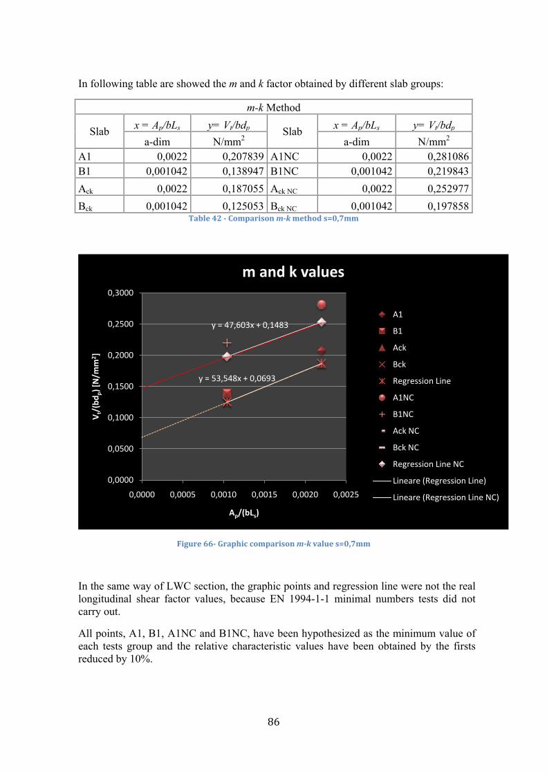
86

In following table are showed the m and k factor obtained by different slab groups:

m-k Method

Slab x = Ap/bLs y= Vt/bdp Slab x = Ap/bLs y= Vt/bdp a-dim N/mm2 a-dim N/mm2

A1 0,0022 0,207839 A1NC 0,0022 0,281086 B1 0,001042 0,138947 B1NC 0,001042 0,219843 Ack 0,0022 0,187055 Ack NC 0,0022 0,252977 Bck 0,001042 0,125053 Bck NC 0,001042 0,197858

Table 42 - Comparison m-k method s=0,7mm

Figure 66- Graphic comparison m-k value s=0,7mm

In the same way of LWC section, the graphic points and regression line were not the real longitudinal shear factor values, because EN 1994-1-1 minimal numbers tests did not carry out.

All points, A1, B1, A1NC and B1NC, have been hypothesized as the minimum value of each tests group and the relative characteristic values have been obtained by the firsts reduced by 10%.

y = 53,548x + 0,0693

y = 47,603x + 0,1483

0,0000

0,0500

0,1000

0,1500

0,2000

0,2500

0,3000

0,0000 0,0005 0,0010 0,0015 0,0020 0,0025

V t/(b

d p) [N

/mm

2 ]

Ap/(bLs)

m and k values

A1

B1

Ack

Bck

Regression Line

A1NC

B1NC

Ack NC

Bck NC

Regression Line NC

Lineare (Regression Line)

Lineare (Regression Line NC)

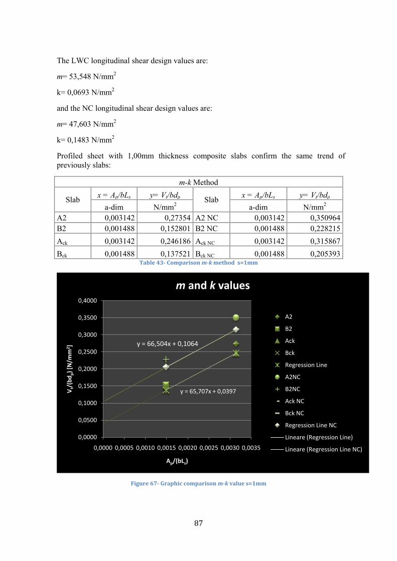
87

The LWC longitudinal shear design values are:

m= 53,548 N/mm2

k= 0,0693 N/mm2

and the NC longitudinal shear design values are:

m= 47,603 N/mm2

k= 0,1483 N/mm2

Profiled sheet with 1,00mm thickness composite slabs confirm the same trend of previously slabs:

m-k Method

Slab x = Ap/bLs y= Vt/bdp Slab x = Ap/bLs y= Vt/bdp a-dim N/mm2 a-dim N/mm2

A2 0,003142 0,27354 A2 NC 0,003142 0,350964 B2 0,001488 0,152801 B2 NC 0,001488 0,228215 Ack 0,003142 0,246186 Ack NC 0,003142 0,315867 Bck 0,001488 0,137521 Bck NC 0,001488 0,205393

Table 43- Comparison m-k method s=1mm

Figure 67- Graphic comparison m-k value s=1mm

y = 65,707x + 0,0397

y = 66,504x + 0,1064

0,0000

0,0500

0,1000

0,1500

0,2000

0,2500

0,3000

0,3500

0,4000

0,0000 0,0005 0,0010 0,0015 0,0020 0,0025 0,0030 0,0035

V t/(b

d p) [N

/mm

2 ]

Ap/(bLs)

m and k values

A2

B2

Ack

Bck

Regression Line

A2NC

B2NC

Ack NC

Bck NC

Regression Line NC

Lineare (Regression Line)

Lineare (Regression Line NC)

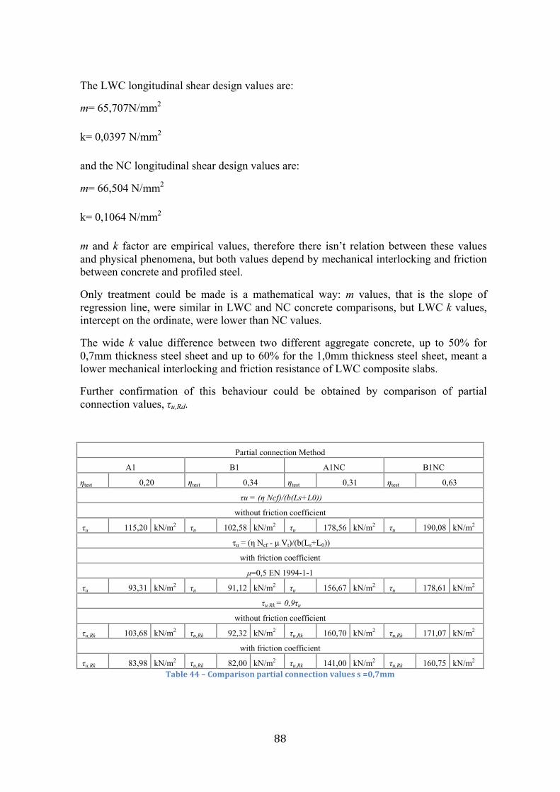
88

The LWC longitudinal shear design values are:

m= 65,707N/mm2

k= 0,0397 N/mm2

and the NC longitudinal shear design values are:

m= 66,504 N/mm2

k= 0,1064 N/mm2

m and k factor are empirical values, therefore there isn’t relation between these values and physical phenomena, but both values depend by mechanical interlocking and friction between concrete and profiled steel.

Only treatment could be made is a mathematical way: m values, that is the slope of regression line, were similar in LWC and NC concrete comparisons, but LWC k values, intercept on the ordinate, were lower than NC values.

The wide k value difference between two different aggregate concrete, up to 50% for 0,7mm thickness steel sheet and up to 60% for the 1,0mm thickness steel sheet, meant a lower mechanical interlocking and friction resistance of LWC composite slabs.

Further confirmation of this behaviour could be obtained by comparison of partial connection values, τu,Rd.

Partial connection Method

A1 B1 A1NC B1NC

ηtest 0,20 ηtest 0,34 ηtest 0,31 ηtest 0,63

τu = (η Ncf)/(b(Ls+L0))

without friction coefficient

τu 115,20 kN/m2 τu 102,58 kN/m2 τu 178,56 kN/m2 τu 190,08 kN/m2

τu = (η Ncf - μ Vt)/(b(Ls+L0))

with friction coefficient

μ=0,5 EN 1994-1-1

τu 93,31 kN/m2 τu 91,12 kN/m2 τu 156,67 kN/m2 τu 178,61 kN/m2

τu,Rk = 0,9τu

without friction coefficient

τu,Rk 103,68 kN/m2 τu,Rk 92,32 kN/m2 τu,Rk 160,70 kN/m2 τu,Rk 171,07 kN/m2

with friction coefficient

τu,Rk 83,98 kN/m2 τu,Rk 82,00 kN/m2 τu,Rk 141,00 kN/m2 τu,Rk 160,75 kN/m2 Table 44 – Comparison partial connection values s =0,7mm

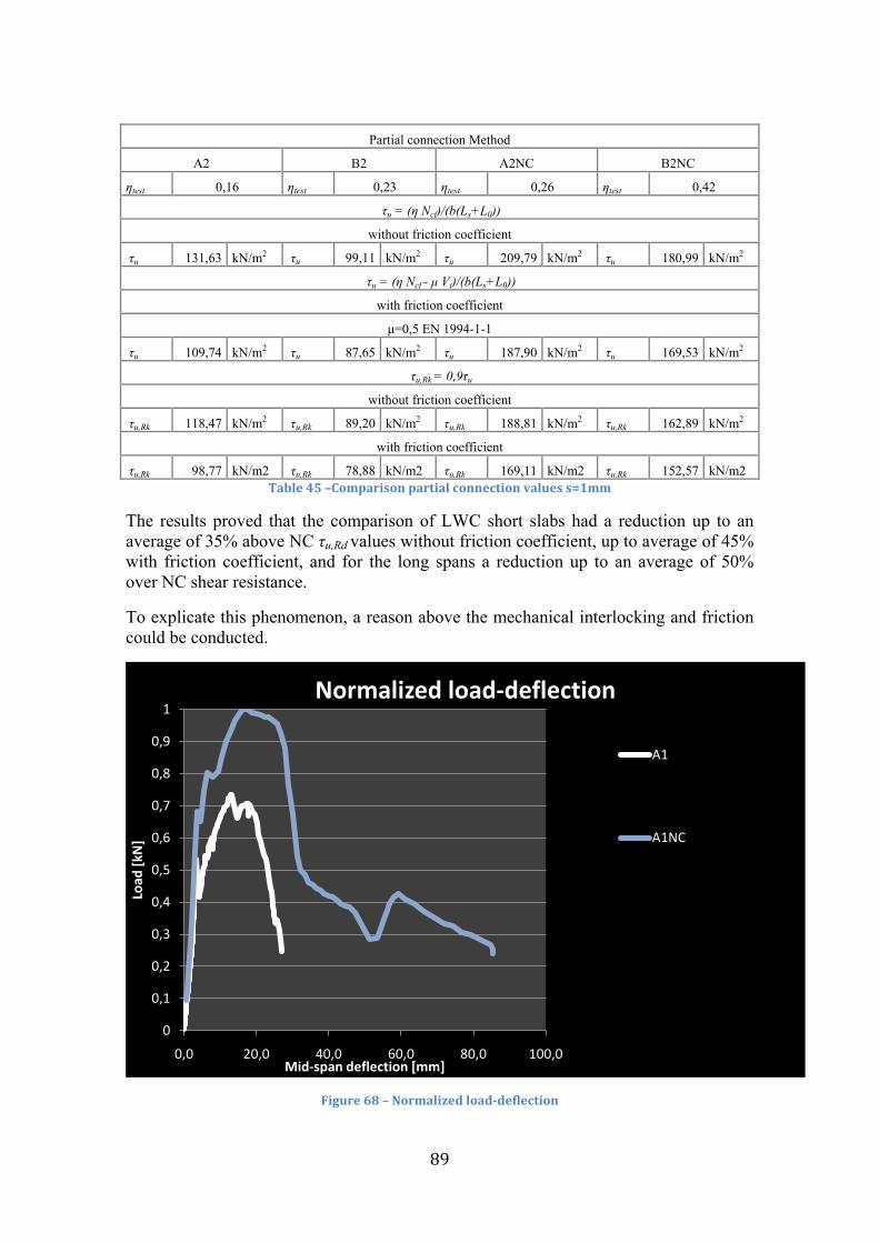
89

Partial connection Method

A2 B2 A2NC B2NC

ηtest 0,16 ηtest 0,23 ηtest 0,26 ηtest 0,42

τu = (η Ncf)/(b(Ls+L0))

without friction coefficient

τu 131,63 kN/m2 τu 99,11 kN/m2 τu 209,79 kN/m2 τu 180,99 kN/m2

τu = (η Ncf - μ Vt)/(b(Ls+L0))

with friction coefficient

μ=0,5 EN 1994-1-1

τu 109,74 kN/m2 τu 87,65 kN/m2 τu 187,90 kN/m2 τu 169,53 kN/m2

τu,Rk = 0,9τu

without friction coefficient

τu,Rk 118,47 kN/m2 τu,Rk 89,20 kN/m2 τu,Rk 188,81 kN/m2 τu,Rk 162,89 kN/m2

with friction coefficient

τu,Rk 98,77 kN/m2 τu,Rk 78,88 kN/m2 τu,Rk 169,11 kN/m2 τu,Rk 152,57 kN/m2 Table 45 –Comparison partial connection values s=1mm

The results proved that the comparison of LWC short slabs had a reduction up to an average of 35% above NC τu,Rd values without friction coefficient, up to average of 45% with friction coefficient, and for the long spans a reduction up to an average of 50% over NC shear resistance.

To explicate this phenomenon, a reason above the mechanical interlocking and friction could be conducted.

Figure 68 – Normalized load-deflection

0

0,1

0,2

0,3

0,4

0,5

0,6

0,7

0,8

0,9

1

0,0 20,0 40,0 60,0 80,0 100,0

Load

[kN

]

Mid-span deflection [mm]

Normalized load-deflection

A1

A1NC

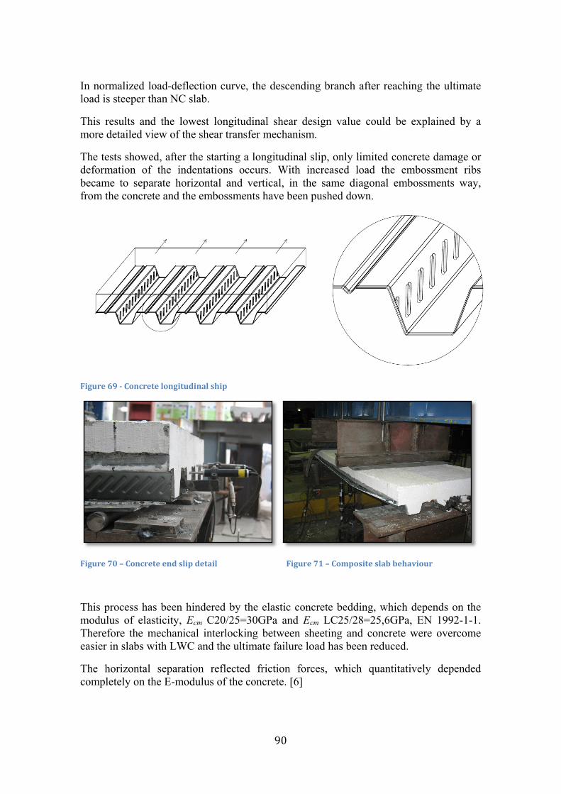
90

In normalized load-deflection curve, the descending branch after reaching the ultimate load is steeper than NC slab.

This results and the lowest longitudinal shear design value could be explained by a more detailed view of the shear transfer mechanism.

The tests showed, after the starting a longitudinal slip, only limited concrete damage or deformation of the indentations occurs. With increased load the embossment ribs became to separate horizontal and vertical, in the same diagonal embossments way, from the concrete and the embossments have been pushed down.

Figure 69 - Concrete longitudinal ship

Figure 70 – Concrete end slip detail Figure 71 – Composite slab behaviour

This process has been hindered by the elastic concrete bedding, which depends on the modulus of elasticity, Ecm C20/25=30GPa and Ecm LC25/28=25,6GPa, EN 1992-1-1. Therefore the mechanical interlocking between sheeting and concrete were overcome easier in slabs with LWC and the ultimate failure load has been reduced.

The horizontal separation reflected friction forces, which quantitatively depended completely on the E-modulus of the concrete. [6]

91

Thus, in case of LWC the loss of mechanical interlock after reaching the maximum load could not be compensated by activation of friction interlock in the same manner as with NC. This initiates the steep descending branch.

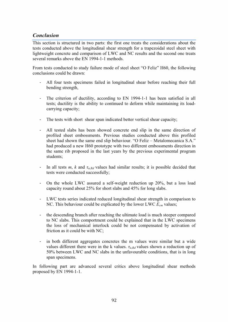
92

Conclusion This section is structured in two parts: the first one treats the considerations about the tests conducted above the longitudinal shear strength for a trapezoidal steel sheet with lightweight concrete and comparison of LWC and NC results and the second one treats several remarks above the EN 1994-1-1 methods.

From tests conducted to study failure mode of steel sheet “O Feliz” H60, the following conclusions could be drawn:

- All four tests specimens failed in longitudinal shear before reaching their full bending strength,

- The criterion of ductility, according to EN 1994-1-1 has been satisfied in all tests; ductility is the ability to continued to deform while maintaining its load-carrying capacity;

- The tests with short shear span indicated better vertical shear capacity;

- All tested slabs has been showed concrete end slip in the same direction of profiled sheet embossments. Previous studies conducted above this profiled sheet had shown the same end slip behaviour. “O Feliz – Metalomecanica S.A.” had produced a new H60 prototype with two different embossments direction in the same rib proposed in the last years by the previous experimental program students;

- In all tests m, k and τu,Rd values had similar results; it is possible decided that tests were conducted successfully;

- On the whole LWC assured a self-weight reduction up 20%, but a loss load capacity round about 25% for short slabs and 45% for long slabs.

- LWC tests series indicated reduced longitudinal shear strength in comparison to NC. This behaviour could be explicated by the lower LWC Ecm values;

- the descending branch after reaching the ultimate load is much steeper compared to NC slabs. This comportment could be explained that in the LWC specimens the loss of mechanical interlock could be not compensated by activation of friction as it could be with NC;

- in both different aggregates concretes the m values were similar but a wide values different there were in the k values. τu,Rd values shown a reduction up of 50% between LWC and NC slabs in the unfavourable conditions, that is in long span specimens.

In following part are advanced several critics above longitudinal shear methods proposed by EN 1994-1-1.

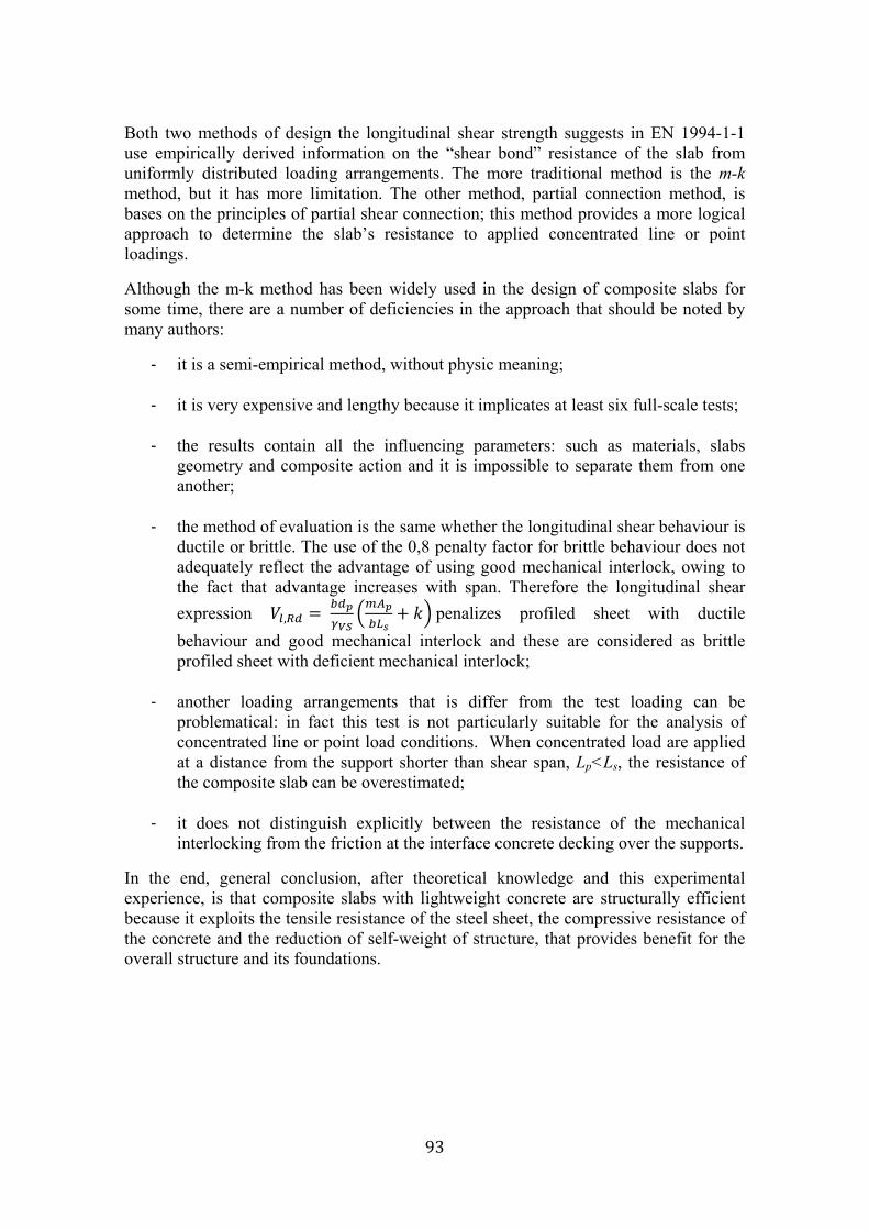
93

Both two methods of design the longitudinal shear strength suggests in EN 1994-1-1 use empirically derived information on the “shear bond” resistance of the slab from uniformly distributed loading arrangements. The more traditional method is the m-k method, but it has more limitation. The other method, partial connection method, is bases on the principles of partial shear connection; this method provides a more logical approach to determine the slab’s resistance to applied concentrated line or point loadings.

Although the m-k method has been widely used in the design of composite slabs for some time, there are a number of deficiencies in the approach that should be noted by many authors:

- it is a semi-empirical method, without physic meaning;

- it is very expensive and lengthy because it implicates at least six full-scale tests;

- the results contain all the influencing parameters: such as materials, slabs geometry and composite action and it is impossible to separate them from one another;

- the method of evaluation is the same whether the longitudinal shear behaviour is ductile or brittle. The use of the 0,8 penalty factor for brittle behaviour does not adequately reflect the advantage of using good mechanical interlock, owing to the fact that advantage increases with span. Therefore the longitudinal shear expression 𝑉𝑙,𝑅𝑑 = 𝑏𝑑𝑝

𝛾𝑉𝑆�𝑚𝐴𝑝𝑏𝐿𝑠

+ 𝑘� penalizes profiled sheet with ductile behaviour and good mechanical interlock and these are considered as brittle profiled sheet with deficient mechanical interlock;

- another loading arrangements that is differ from the test loading can be problematical: in fact this test is not particularly suitable for the analysis of concentrated line or point load conditions. When concentrated load are applied at a distance from the support shorter than shear span, Lp<Ls, the resistance of the composite slab can be overestimated;

- it does not distinguish explicitly between the resistance of the mechanical interlocking from the friction at the interface concrete decking over the supports.

In the end, general conclusion, after theoretical knowledge and this experimental experience, is that composite slabs with lightweight concrete are structurally efficient because it exploits the tensile resistance of the steel sheet, the compressive resistance of the concrete and the reduction of self-weight of structure, that provides benefit for the overall structure and its foundations.

94

References [1] C. K. Wong - Feasibility studies of two-way composite steel-deck Thesis in civil engineering 1987 [2] A. Short, W. Kinninburgh - Lightweigth concrete

Cr books LTD, 1968 [3] European unite - Eurolightcon – Light weight aggregate Brite EuRam III, 2000 [4] L. Calado, J. Santos - Strutura mista de aço e betão Ist press, 2010 [5] R. Carmona - Avaliação do comportamento experimental de lajes mistas aço-

betão com cofragem metalica colaborante Dissertação apresentada para a obtenção do grau de mestre em engenharia civil,

2009 [6] T. Faust - Lightweigth Concrete in Composite Structures Lacer n.2, 1997 Books: P. Kumar, P. Monteiro - Concrete, microstructure, properties and materials Mc Graw-Hill 2007 A. Short, W. Kinninburgh - Lightweigth concrete Cr books LTD, 1968 R.P. Johnson - Composite Structures of Steel and Concrete Beams, slabs, columns, and frames for buildings Volume 1, Blackwell Scientific Publication, 2004 J. Lourenço, E. Julio, P. Maranha - Betões de agregados leves de argila expandida – Guia para a sua utilizaçao Apeb, 2008 J. Rackham, G. Couchman, S. Hicks - Composite slabs and beams using steel decking: best practice for design and construction The metal cladding e roofing manufacturers association, 2009 SSEDTA - Structural steelwork eurocodes development of a trans-national approach 2001 R. Simões – Manual de dimensionamento de estruturas metalicas CMM, 2007

95

Articles: Z. Nagy, I. Szatmari - Composite slab design Tecnical University of Budapest, Department of steel structure, 1998 S. Hicks - Composite slabs The steel construction institute, 2008 D. Lam, J. Qureshi - Prediction of longitudinal shear resistance of composite slabs with profile sheeting to eurocode 4 The Regency Steel Asia International Symposium on innovations in structural steel, RSA-ISISS 2008 Thesis: I. Shobaki - The behaviour of profiled steel sheet/concrete composite slabs University of Salford, UK, 2000 European Standards: CEN - UNI EN 1990:2006 : Eurocode 0 - Basis of structural design- European Committee for Standardization, 2006 CEN, UNI EN 1991-1-6:2005: Eurocode 1 - Actions on structures - Part 1-6: General actions - Actions during execution European Committee for Standardization, 2005 CEN, UNI EN 1992-1-1:2005: Eurocode 2 - Design of concrete structures - Part 1-1: General rules and rules for buildings European Committee for Standardization, 2005 CEN, UNI EN 1993-1-3:2007: Eurocode 3 - Design of steel structures - Part 1-3: General rules - Supplementary rules for cold-formed members and sheeting European Committee for Standardization, 2007 CEN, UNI EN 1994-1-1:2005: Eurocode 4 - Design of composite steel and concrete structures - Part 1-1: General rules and rules for buildings European Committee for Standardization, 2005 Istituto portugues da Qualidade, PT EN 993-1:2000: Ensaios das propriedades geometricas dos agregados Parte 1: Analise granulometrica - Metodo de peneiração European Committee for Standardization, 2000 CEN, EN 13055-1:2002: Lightweight aggregates Part 1: Lightweight aggregates for concrete, mortar and grout European Committee for Standardization, 2002

96

Istituto portugues da Qualidade, PT EN 206-1:2007: Betão Parte 1: Especificação, desempenho, produção e conformidade European Committee for Standardization, 2007 ISO, ISO 6784:1982 Concrete - Determination of static modulus of elasticity in compression International organization for standard, 1982

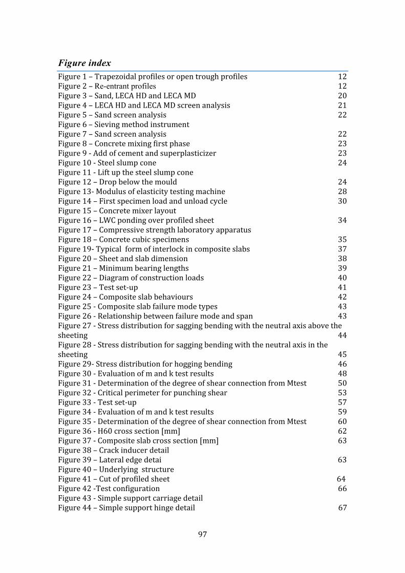
97

Figure index Figure 1 – Trapezoidal profiles or open trough profiles 12 Figure 2 – Re-entrant profiles 12 Figure 3 – Sand, LECA HD and LECA MD 20 Figure 4 – LECA HD and LECA MD screen analysis 21 Figure 5 – Sand screen analysis 22 Figure 6 – Sieving method instrument Figure 7 – Sand screen analysis 22 Figure 8 – Concrete mixing first phase 23 Figure 9 - Add of cement and superplasticizer 23 Figure 10 - Steel slump cone 24 Figure 11 - Lift up the steel slump cone Figure 12 – Drop below the mould 24 Figure 13- Modulus of elasticity testing machine 28 Figure 14 – First specimen load and unload cycle 30 Figure 15 – Concrete mixer layout Figure 16 – LWC ponding over profiled sheet 34 Figure 17 – Compressive strength laboratory apparatus Figure 18 – Concrete cubic specimens 35 Figure 19- Typical form of interlock in composite slabs 37 Figure 20 – Sheet and slab dimension 38 Figure 21 – Minimum bearing lengths 39 Figure 22 – Diagram of construction loads 40 Figure 23 – Test set-up 41 Figure 24 – Composite slab behaviours 42 Figure 25 - Composite slab failure mode types 43 Figure 26 - Relationship between failure mode and span 43 Figure 27 - Stress distribution for sagging bending with the neutral axis above the sheeting 44 Figure 28 - Stress distribution for sagging bending with the neutral axis in the sheeting 45 Figure 29- Stress distribution for hogging bending 46 Figure 30 - Evaluation of m and k test results 48 Figure 31 - Determination of the degree of shear connection from Mtest 50 Figure 32 - Critical perimeter for punching shear 53 Figure 33 - Test set-up 57 Figure 34 - Evaluation of m and k test results 59 Figure 35 - Determination of the degree of shear connection from Mtest 60 Figure 36 - H60 cross section [mm] 62 Figure 37 - Composite slab cross section [mm] 63 Figure 38 – Crack inducer detail Figure 39 – Lateral edge detai 63 Figure 40 – Underlying structure Figure 41 – Cut of profiled sheet 64 Figure 42 -Test configuration 66 Figure 43 - Simple support carriage detail Figure 44 – Simple support hinge detail 67

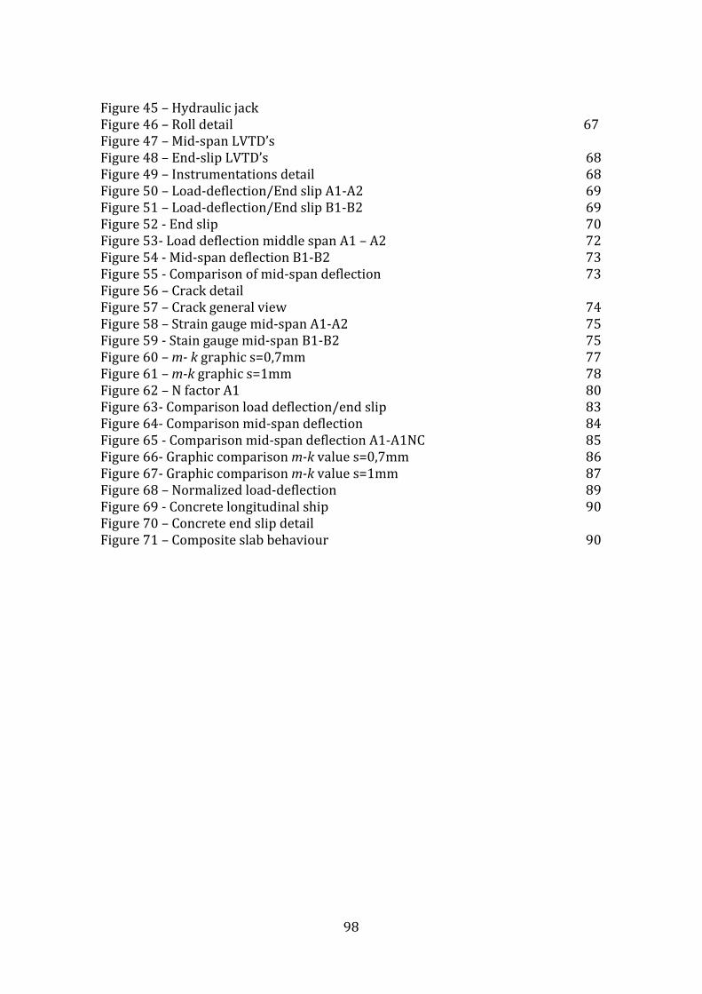
98

Figure 45 – Hydraulic jack Figure 46 – Roll detail 67 Figure 47 – Mid-span LVTD’s Figure 48 – End-slip LVTD’s 68 Figure 49 – Instrumentations detail 68 Figure 50 – Load-deflection/End slip A1-A2 69 Figure 51 – Load-deflection/End slip B1-B2 69 Figure 52 - End slip 70 Figure 53- Load deflection middle span A1 – A2 72 Figure 54 - Mid-span deflection B1-B2 73 Figure 55 - Comparison of mid-span deflection 73 Figure 56 – Crack detail Figure 57 – Crack general view 74 Figure 58 – Strain gauge mid-span A1-A2 75 Figure 59 - Stain gauge mid-span B1-B2 75 Figure 60 – m- k graphic s=0,7mm 77 Figure 61 – m-k graphic s=1mm 78 Figure 62 – N factor A1 80 Figure 63- Comparison load deflection/end slip 83 Figure 64- Comparison mid-span deflection 84 Figure 65 - Comparison mid-span deflection A1-A1NC 85 Figure 66- Graphic comparison m-k value s=0,7mm 86 Figure 67- Graphic comparison m-k value s=1mm 87 Figure 68 – Normalized load-deflection 89 Figure 69 - Concrete longitudinal ship 90 Figure 70 – Concrete end slip detail Figure 71 – Composite slab behaviour 90

99

Table index

Table 1 – Sand, LECA HD and LECA MD screen analysis 21 Table 2 - Mix design 23 Table 3 - Slump test results 25 Table 4 - Total aggregate moisture content 25 Table 5 - Compressive strength results, March 15th 26 Table 6 - Compressive strength results, March 30th 27 Table 7 - Density class 28 Table 8 - Modulus of elasticity results 30 Table 9 - Compressive strength results, March 31st 31 Table 10 - Concrete class strength 31 Table 11 - Mix design with relative humidity 32 Table 12 - Concrete volume 33 Table 13 - Mix design 80l 34 Table 14 – Compressive strength results, April 22nd 34 Table 15 – Compressive strength result, May 14th 35 Table 16 - Strength classes for Lightweight concrete 36 Table 17 – Compressive strength class criterions 36 Table 18 – Slab-beam behaviour 38 Table 19 – Bearing requirements 39 Table 20 – Table of construction loads 40 Table 21 - Span length 49 Table 22 - Slabs geometric characteristics 62 Table 23 – Compressive strength result, test day 64 Table 24 - Compressive strength class criterions 64 Table 25 - H60 profiled sheet characteristics 65 Table 26 – Composite slab behaviours 70 Table 27 – Geometric characteristics and load test value 71 Table 28 - Test values 71 Table 29 - Profiled sheet plastic deformation 74 Table 30 - Geometric characteristics composite slab 76 Table 31- Test results 76 Table 32 – m-k method s=0,7mm 77 Table 33 – m-k method 78 Table 34 – Flexure A1 79 Table 35 – Test bending A1 79 Table 36 - Partial connection value A1 79 Table 37 - Partial connection factors A1 80 Table 38 - Partial connection factors A2-B1-B2 81 Table 39 - NC composite slab behaviour 84 Table 40 - Comparison test values 84 Table 41- NC geometric characteristic and test values 85 Table 42 - Comparison m-k method s=0,7mm 86 Table 43- Comparison m-k method s=1mm 87 Table 44 – Comparison partial connection values s =0,7mm 88

100

Table 45 –Comparison partial connection values s=1mm 89