arX

iv:1

908.

0865

7v1

[he

p-ph

] 2

3 A

ug 2

019

Transverse momentum dependent parton distributions of pion in

the light-front holographic model

Navdeep Kaur and Harleen Dahiya

Department of Physics, Dr. B. R. Ambedkar National

Institute of Technology, Jalandhar-144011, India

Abstract

Using the light-front holographic model, we study the transverse momentum dependent parton

distributions (TMDs) for the case of pion. At leading twist, the unpolarized parton distribution

function f1π(x,k2⊥) and the Boer-Mulders function h⊥1π(x,k

2⊥) are obtained for pion. We calculate

both the functions using the light-front holographic model with spin improved wave function

and compare the predicted results with available results of other models. In order to provide

inputs in predicting future experimental data, a LO evolution is performed from model scale to

experimental scale for the case of unpolarized parton distribution function f1π(x,k2⊥).

1

I. INTRODUCTION

Understanding the hadronic structure in terms of its constituents has become the ma-

jor goal of high energy physics during the last few decades. A lot of experimental as well

as theoretical efforts are continuously being made to explore the three-dimensional (3D)

picture of hadrons in configuration and momentum space. A one-dimensional picture of

hadron is provided by the parton distribution functions (PDFs) which describe the prob-

ability of finding a parton (quark or gluon) with longitudinal momentum fraction inside

the hadron in forward scattering region. By extending the PDFs from forward scattering

region to off-forward scattering region, one can obtain the generalized parton distributions

(GPDs). The GPDs not only provide the information about the longitudinal momentum

fraction of parton but also give the longitudinal momentum transfer between the initial

and final state of hadron [1]. The various scattering process like deep virtual Compton

scattering (DVCS), deep virtual meson production (DVMP) provide detailed information

on the GPDs [2–9]. Further, the study of transverse momentum dependent parton distri-

bution function (TMDs) provide the 3D picture of the hadrons and related information

about the correlation between the spin of parent hadron and the intrinsic transverse mo-

mentum of its constituent partons [10–14]. In recent years, several experiments have been

running and are being planned for future to gather such information.

The TMDs of hadrons can be measured experimentally in semi-inclusive deep inelastic

scattering (SIDIS) [14, 15] and Drell-Yan (DY) processes [16–20]. TMDs allow us to

access the partonic configuration of hadrons with longitudinal momentum fraction x and

transverse momentum k⊥. Apart from x and k⊥, TMDs also depend on the Wilson

line (gauge link). The presence of Wilson line in TMD correlator is necessary to attain

color gauge invariance and to obtain non-zero T-odd TMDs (Sivers and Boer-Mulders

functions). Wilson lines are process dependent so their presence in TMD correlator makes

T-odd TMDs process dependent. In the case of SIDIS process final state interaction

(FSI) and in the case of DY process the initial state interaction between struck quark and

spectator via one gluon exchange are necessary for obtaining non-vanishing T-odd TMDs

[22–27].

2

Pion being the simplest QCD bound state of quark and antiquark among the hadrons,

has attracted lot of attention and also they have the advantage of being probed experimen-

tally. In DY process, the structure of pion can be probed by hitting them on nuclear target

[28–31]. In past years, lot of theoretical work has been done to explore the pion structure

including the studies on pion PDFs in the light-front constituent model, chiral constituent

quark model [32–34], Nambu-Jone-Lasino model and using DysonâĂŞSchwinger equation

[35, 36] and Bethe-Salpeter wave functions. GPDs of pion have also been studied ex-

tensively in various other models [37–46]. Recently pion TMDs have been calculated in

light-front constituent approach [47, 48], spectator model [49–51], in NJL model [53] and

in AdS/QCD approach [54, 55].

To study 3D structure of hadrons theoretically, hadronic wave functions in terms of

quark and gluons degree of freedom are important. There have been several attempts

in different models to obtain the hadronic wave function, the most recent being the

AdS/QCD correspondence in light-front formalism. By holographic mapping between

the Hamiltonian formulation for quantized QCD and specific properties for hadron in

five-dimensional AdS-space one can obtain the hadronic wave function in light-front holo-

graphic model. The solution of the holographic Schrödinger equation for meson within the

semiclassical approximation of light-front QCD yields the valence meson wave function for

massless quarks [56–59]. For non-vanishing quark masses, there is a need to go beyond the

semiclassical approximation [60]. This has been done by including a perturbation mass

term to the effective potential of the holographic Schrödinger equation [61–64]. Within

the semiclassical approximation of light-front QCD, the dynamical spin effects are usually

neglected. For pion, such effects have been taken into account in recent work [65, 66].

In order to study the spin structure of pion, we have used the holographic light-front

wave function with dynamical spin from the light-front holographic model [66] which in-

cludes the higher helicity (parallel spin of partons) components besides the usual lower

helicity (anti-parallel spin of partons) components. The higher helicity components may

have the possibility to provide non-leading contribution in the light-front wave-function.

The main motivation to choose this model is the presence of spin wave function in holo-

graphic light-front wave-functions which is not usually present in the original AdS/QCD

3

model but is necessary to obtain the Boer-Mulders function of pion. This model gives a

simultaneous successful description of wide range of experiment data including the decay

constant, the charge radius and EM form factor of pion [66].

In the present work, we predict the results for pion TMDs in light-front holographic

with spin-improved wave function. At leading twist, the pion transverse dependent quark-

quark correlator consists of two TMDs, the unpolarized parton distribution function

f q1π(x,k

2⊥) and the Boer-Mulders function h⊥1π(x,k

2⊥). The TMD f q

1π(x,k2⊥) has been

obtained from the lowest order correlation function. We have compared our result with

the previous results from light-front constituent model [47] and soft wall AdS/QCD [55].

To obtain the function h⊥1π(x,k2⊥), we have used the higher order correlation function

to consider the contribution from the one-gluon exchange between quark and antiquark.

The obtained h⊥1π(x,k2⊥) function has also been compared with the results of light-front

constituent model. In context of experimental observations, the evolution of TMDs are

very crucial for future comparisons. However, as the exact evolution equation for the

Boer-Mulders functions is still under study, we present here the case for only the unpolar-

ized parton distribution function f q1π(x,k

2⊥). We show how it evolves from initial model

scale to higher energy scale using the evolution equation.

The outline of this paper is as follows. In Section II, we discuss the light-front ampli-

tudes in terms of pion light-front wave functions(LFWFs) with different orbital angular

momentum components. In Section III, the unpolarized parton distribution function of

pion is predicted at model scale. The Boer-Mulders function of pion is given in Section

IV. In Section V we discuss the TMD evolution of the unpolarized parton distribution

function. We summarize and conclude our results in Section VI.

II. LIGHT-FRONT AMPLITUDES OF THE PION IN LIGHT-FRONT HOLO-

GRAPHIC MODEL

For the description of a hadron in the light-front dynamics, the classification of in-

dependent wave-function amplitudes with a particular parton combination is necessary.

With the information about the parton content of a hadron, one can obtain the light-

4

front amplitudes for a hadron. The light-front amplitudes of a pion with helicity Λ can be

written in terms of total parton helicity λ and total orbital angular momentum of partons

Lz . With the lowest quark-antiquark Fock state component, the total parton helicity of

pion can be either 0 or 1. Correspondingly, according to law of conservation of angular

momentum, Λ = λ + Lz . Therefore, two light-front wave function amplitudes with total

quark orbital momentum Lz = 0 and | Lz |= 1 exist for a pion with valence |qq〉 Fock

state. The light-front wave function for the quark-antiquark Fock state of a positively

charged pion with momentum P can be written as the superposition of these light-front

amplitudes as follows

|π+(P )〉 = |π+(P )〉Lz=0 + |π+(P )〉|Lz|=1 ,

|π+(P )〉Lz=0 =

∫

d2k⊥

16π3

dx√

6x(1− x)Ψ(0)

π (x,k⊥)3

∑

a=1

[

b†au↑(1)d†ad↓(2)− b†au↓(1)d

†ad↑(2)

]

|0〉,

|π+(P )〉|Lz|=1 =

∫

d2k⊥

16π3

dx√

2x(1− x)Ψ(1)

π (x,k⊥)

×(kx + iky√

3

3∑

a=1

b†au↑(1)d†ad↑(2) |0〉 +

kx − iky√3

3∑

a=1

b†au↓(1)d†ad↓(2) |0〉

)

, (1)

where 1 = (x,k⊥) and 2 = ((1 − x),−k⊥) are the coordinates of quark and antiquark

respectively. Here Ψ(0)π (x,k⊥) and Ψ

(1)π (x,k⊥) are the pion LFWFs for total quark orbital

momentum Lz = 0 and | Lz |= 1 respectively. The creation (annihilation) operators of

u-quark and d-quark with color a are b†aλ (baλ) and d†aλ (daλ) respectively.

The pion state with leading |qq〉 Fock state component can also be written as [67]

|π+(P )〉 =∑

λi

∫

d2k⊥

16π3

dx√

x(1 − x)ΨLz

π (xi,ki⊥;λi)δij√3b†auλ1

(1)d†adλ2(2)|0〉, (2)

where xi and ki⊥ are the longitudinal momentum fraction and transverse momentum of

constituents (quark and antiquark) of pion, respectively. The LFWF ΨLzπ (xi,ki⊥;λi) in

Eq. (2) can be constructed as the product of a momentum-dependent wave function and

a spin-dependent wave function. We have

ΨLz

π (xi,ki⊥;λi) = ψπ(x,k⊥)φπ(λ1, λ2). (3)

5

For the momentum-dependent part of wave function, we choose the light front holographic

wave function of meson as

ψπ(x,k⊥) =4πN0

κ√

x(1− x)exp

[

− k2⊥ +m2

2κ2x(1− x)

]

. (4)

Here N0 is the normalization constant, κ is the scale parameter and m is the quark mass.

The spin dependent part of wave function is defined as

φπ(λ1, λ2) =uλ1

(x,k⊥)√x

[

AMP

2P+γ+γ5 +Bγ5

]

vλ2(x,k⊥)√x

. (5)

Here A and B are constants whose values are constrained by the decay constant and

charged radii of pion. In the present work we use A = 1 and B = 1 following Ref.

[65] as the results of decay constant and radius of charged pion obtained in this case are

comparable with experimental results.

The spin wave function with different helicities of quark and antiquark can be expressed

as

φπ(↑, ↑) = − k1 − ik2x(1 − x)

,

φπ(↑, ↓) =m

x(1− x)+Mπ,

φπ(↓, ↑) = − m

x(1 − x)−Mπ,

φπ(↓, ↓) = − k1 + ik2x(1 − x)

, (6)

where Mπ is the mass of pion. Using the above expressions in Eq. (2) and comparing

it with Eq. (1), the LFWFs for pion state can be mapped out into different angular-

momentum components as follows

Ψ(0)π (x,k⊥) = −m+Mπx(1− x)√

2x(1 − x)ψπ(x,k⊥),

Ψ(1)π (x,k⊥) = − 1√

2x(1− x)ψπ(x,k⊥). (7)

6

III. TRANSVERSE MOMENTUM DEPENDENT PARTON DISTRIBUTION

FUNCTIONS (TMDS) OF PION

The quark transverse momentum distributions (TMDs) can be obtained by using

quark-quark correlator for SIDIS [21, 68, 69]

Φ(x,k⊥)[Γ] =

∫

dy−d2y⊥

2π3 eik.y〈π(P )|ψ(0)W[ 0 |∞, 0, 0T ]W[∞, y+, yT | y ]ψ(y)|π(P )〉∣

∣

∣

y+=0,

(8)

where Γ is the Dirac operator, k is the momentum of the struck quark inside the pion of

momentum P and x = p+/P+ is the longitudinal momentum fraction carried by struck

quark. Here W is the gauge link operator or Wilson line which makes the correlation

function gauge-invariant. Wilson line connects the two quark fields ψ at different points

0 and y and is defined as

W[0|y] = P exp(

− ig

∫ y

0

dηµAµ(η))

, (9)

where Aµ represents the gauge field.

At leading twist, the transverse structure of pion is described by two TMDs: the

unpolarized parton distribution function f q1π(x,k

2⊥) (also called T-even TMD) and the

Boer-Mulders function h⊥1π(x,k2⊥) (also called T-odd TMD). The leading twist pion TMDs

can be parametrized from the correlator given in Eq. (8) and we have

1

2Φ[γ+] = f1π(x,k

2⊥),

1

2Φ[iσj+γ5] =

εijkj⊥Mπ

h⊥1π(x,k2⊥). (10)

A. Unpolarised parton distribution function of pion

The unpolarized distribution function f q1π(x,k

2⊥) describes the probability of finding

a quark with longitudinal momentum fraction x and transverse momentum k⊥ inside an

unpolarized pion. One can obtain f q1π(x,k

2⊥) from the lowest order correlation function

[70] (without Wilson line) and we have

f q1π(x,k

2⊥) =

∫

dy−d2y⊥

2π3 ei(y−k+−y⊥.k⊥) 〈π(P )|ψ(0) γ+ ψ(y)|π(P )〉

∣

∣

∣

y+=0. (11)

7

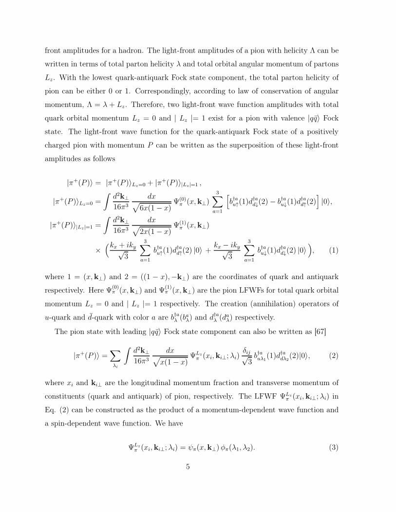
FIG. 1: 3D plot of unpolarized TMD of pionf q1π(x,k

2⊥) as a function of x and k2

⊥.

Using the light-front state of pion given in Eq. (1) and the quark fields in terms of Fock

operators, the unpolarized quark distribution f q1π(x,k

2⊥) of pion can be expressed as the

overlap of LFWFs given in Eq. (7) as

f q1π(x,k

2⊥) =

1

(2π)3[

|ψ(0)π (x,k⊥)|2 + k2

⊥ |ψ(1)π (x,k⊥)|2

]

. (12)

On solving analytically, we have the unpolarized parton distribution function of pion as

f q1π(x,k

2⊥) =

N20

π

[k2⊥ + (m+ x(1− x)M)2]

κ2 x3 (1− x)3exp

[

− k2⊥ +m2)

κ2x(1 − x)

]

. (13)

After integration over k⊥, the unpolarized distribution function f q1π(x,k

2⊥) reduces to

parton distribution function fπ(x). The parton distribution function fπ(x) satisfies the

normalization condition∫

dxfπ(x) = 1. (14)

It would be important to mention here that, in this model, the distribution f q1π(x,k

2⊥) of

quark with longitudinal momentum fraction x, is equal to the distribution f q1π(1− x,k2

⊥)

of an antiquark with longitudinal momentum fraction 1− x inside the pion.

To obtain the numerical results of TMDs we need 3 parameters: the scale constant

κ, mass of the quark m and mass of the pion Mπ. We have used the following set of

parameters following Ref. [66]

κ = 523 MeV, m = 330 MeV and Mπ = 139 MeV. (15)

8

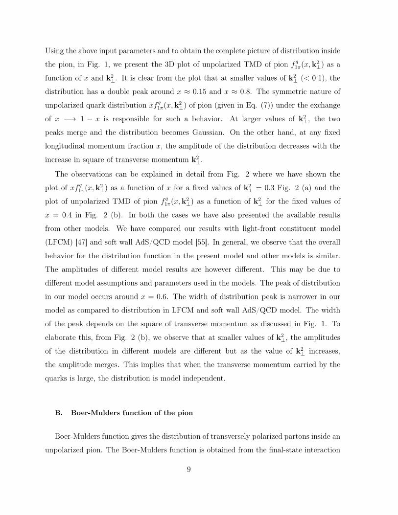
Using the above input parameters and to obtain the complete picture of distribution inside

the pion, in Fig. 1, we present the 3D plot of unpolarized TMD of pion f q1π(x,k

2⊥) as a

function of x and k2⊥. It is clear from the plot that at smaller values of k2

⊥ (< 0.1), the

distribution has a double peak around x ≈ 0.15 and x ≈ 0.8. The symmetric nature of

unpolarized quark distribution xf q1π(x,k

2⊥) of pion (given in Eq. (7)) under the exchange

of x −→ 1 − x is responsible for such a behavior. At larger values of k2⊥, the two

peaks merge and the distribution becomes Gaussian. On the other hand, at any fixed

longitudinal momentum fraction x, the amplitude of the distribution decreases with the

increase in square of transverse momentum k2⊥.

The observations can be explained in detail from Fig. 2 where we have shown the

plot of xf q1π(x,k

2⊥) as a function of x for a fixed values of k2

⊥ = 0.3 Fig. 2 (a) and the

plot of unpolarized TMD of pion f q1π(x,k

2⊥) as a function of k2

⊥ for the fixed values of

x = 0.4 in Fig. 2 (b). In both the cases we have also presented the available results

from other models. We have compared our results with light-front constituent model

(LFCM) [47] and soft wall AdS/QCD model [55]. In general, we observe that the overall

behavior for the distribution function in the present model and other models is similar.

The amplitudes of different model results are however different. This may be due to

different model assumptions and parameters used in the models. The peak of distribution

in our model occurs around x = 0.6. The width of distribution peak is narrower in our

model as compared to distribution in LFCM and soft wall AdS/QCD model. The width

of the peak depends on the square of transverse momentum as discussed in Fig. 1. To

elaborate this, from Fig. 2 (b), we observe that at smaller values of k2⊥, the amplitudes

of the distribution in different models are different but as the value of k2⊥ increases,

the amplitude merges. This implies that when the transverse momentum carried by the

quarks is large, the distribution is model independent.

B. Boer-Mulders function of the pion

Boer-Mulders function gives the distribution of transversely polarized partons inside an

unpolarized pion. The Boer-Mulders function is obtained from the final-state interaction

9

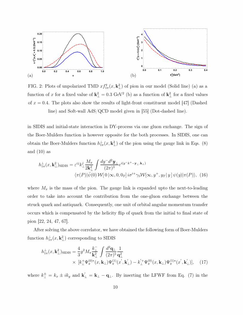
(a) (b)

FIG. 2: Plots of unpolarized TMD xf q1π(x,k

2⊥) of pion in our model (Solid line) (a) as a

function of x for a fixed value of k2⊥ = 0.3 GeV2 (b) as a function of k2

⊥ for a fixed values

of x = 0.4. The plots also show the results of light-front constituent model [47] (Dashed

line) and Soft-wall AdS/QCD model given in [55] (Dot-dashed line).

in SIDIS and initial-state interaction in DY-process via one gluon exchange. The sign of

the Boer-Mulders function is however opposite for the both processes. In SIDIS, one can

obtain the Boer-Mulders function h⊥1π(x,k2⊥) of the pion using the gauge link in Eqs. (8)

and (10) as

h⊥1π(x,k2⊥)SIDIS = εijkj⊥

Mπ

2k2⊥

∫

dy−d2y⊥

(2π)3ei(y

−k+−y⊥.k⊥)

〈π(P )|ψ(0)W[ 0 |∞, 0, 0T ] iσi+γ5W[∞, y+, yT | y ]ψ(y)|π(P )〉, (16)

where Mπ is the mass of the pion. The gauge link is expanded upto the next-to-leading

order to take into account the contribution from the one-gluon exchange between the

struck quark and antiquark. Consequently, one unit of orbital angular momentum transfer

occurs which is compensated by the helicity flip of quark from the initial to final state of

pion [22, 24, 47, 67].

After solving the above correlator, we have obtained the following form of Boer-Mulders

function h⊥1π(x,k2⊥) corresponding to SIDIS

h⊥1π(x,k2⊥)SIDIS =

4

3g2Mπ

k−⊥k2⊥

∫

d2q⊥

(2π)51

q2⊥

× [k+⊥Ψ(0)∗π (x,k⊥)Ψ

(1)π (x

′

,k′

⊥)− k′+⊥ Ψ(0)

π (x,k⊥)Ψ(1)∗π (x

′

,k′

⊥)], (17)

where k±⊥ = kx ± iky and k′

⊥ = k⊥ − q⊥. By inserting the LFWF from Eq. (7) in the

10

FIG. 3: 3D plot of Boer-Mulders function h⊥1π(x,k2⊥) in DY-process as a function of x

and k2⊥.

above equation, the following analytic expression for h⊥1π(x,k2⊥) can be derived

h⊥1π(x,k2⊥)SIDIS =

4

3g2Mπ

(4πN0)2

k2⊥

× (m+Mπx(1− x))2

2x2(1− x)2

[

1− exp

[

k2⊥

2κ2x(1 − x)

]

]

exp

[

− k2⊥ +m2

κ2x(1 − x)

]

.(18)

Here g is the parameter related to the coupling constant as g2 = 4παs(µ0). We have ob-

tained the result for Boer-Mulders function h⊥1π(x,k2⊥) of pion in DY-process by changing

the sign i.e. h⊥1π(x,k2⊥)DY = −h⊥1π(x,k2

⊥)SIDIS. The model calculation is constrained by the

model-independent positivity relation of unpolarized TMD and Boer-Mulders function is

defined as

P π(x,k2⊥) ≡ f1π(x,k

2⊥)−

k⊥

Mπ

|h⊥1π(x,k2⊥)| ≥ 0. (19)

We have presented the 3D plot of Boer-Mulders function in DY-process as a function

of x and k2⊥ in Fig. 3. The amplitude of h⊥1π(x,k

2⊥) decreases with the increase in k2

⊥

for any fixed value of x. This implies that the probability of finding the quarks with

transverse spin inside the pion is less when they carry large transverse momentum. At

smaller values of k2⊥, a double peak is observed similar to the case of unpolarized quark

distribution which is because of the symmetric nature of Boer-Mulders function under

the exchange of x −→ 1 − x. Our results are in agreement with the results for pion

Boer-Mulders function in light-front constituent approach [47].

11

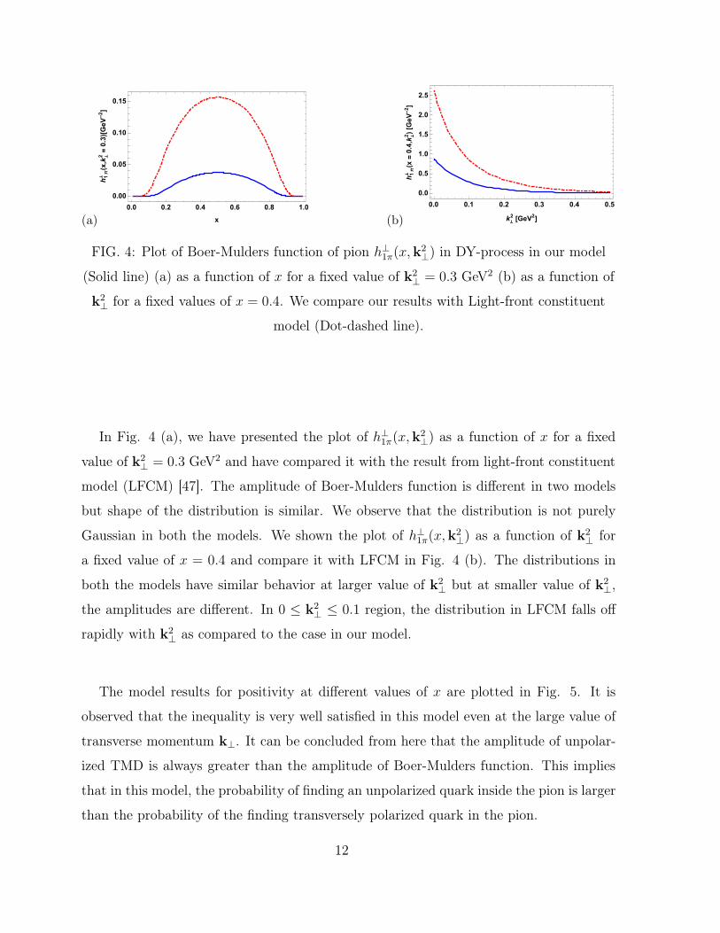
(a) (b)

FIG. 4: Plot of Boer-Mulders function of pion h⊥1π(x,k2⊥) in DY-process in our model

(Solid line) (a) as a function of x for a fixed value of k2⊥ = 0.3 GeV2 (b) as a function of

k2⊥ for a fixed values of x = 0.4. We compare our results with Light-front constituent

model (Dot-dashed line).

In Fig. 4 (a), we have presented the plot of h⊥1π(x,k2⊥) as a function of x for a fixed

value of k2⊥ = 0.3 GeV2 and have compared it with the result from light-front constituent

model (LFCM) [47]. The amplitude of Boer-Mulders function is different in two models

but shape of the distribution is similar. We observe that the distribution is not purely

Gaussian in both the models. We shown the plot of h⊥1π(x,k2⊥) as a function of k2

⊥ for

a fixed value of x = 0.4 and compare it with LFCM in Fig. 4 (b). The distributions in

both the models have similar behavior at larger value of k2⊥ but at smaller value of k2

⊥,

the amplitudes are different. In 0 ≤ k2⊥ ≤ 0.1 region, the distribution in LFCM falls off

rapidly with k2⊥ as compared to the case in our model.

The model results for positivity at different values of x are plotted in Fig. 5. It is

observed that the inequality is very well satisfied in this model even at the large value of

transverse momentum k⊥. It can be concluded from here that the amplitude of unpolar-

ized TMD is always greater than the amplitude of Boer-Mulders function. This implies

that in this model, the probability of finding an unpolarized quark inside the pion is larger

than the probability of the finding transversely polarized quark in the pion.

12

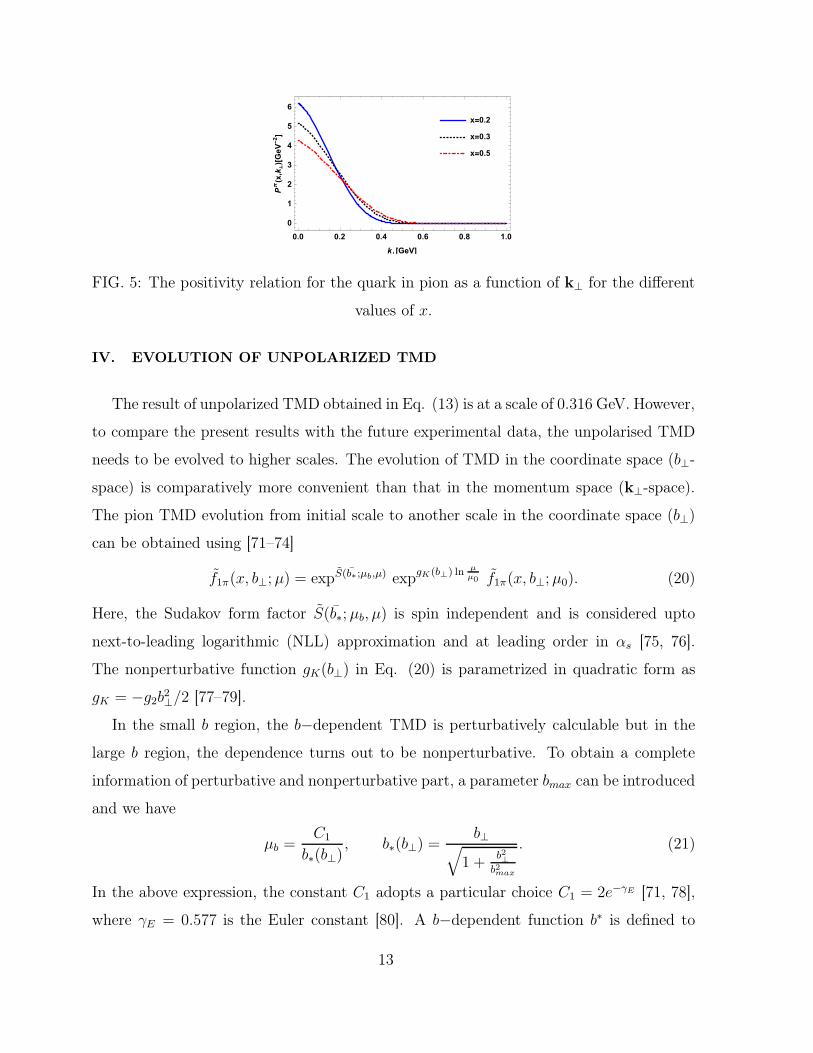
FIG. 5: The positivity relation for the quark in pion as a function of k⊥ for the different

values of x.

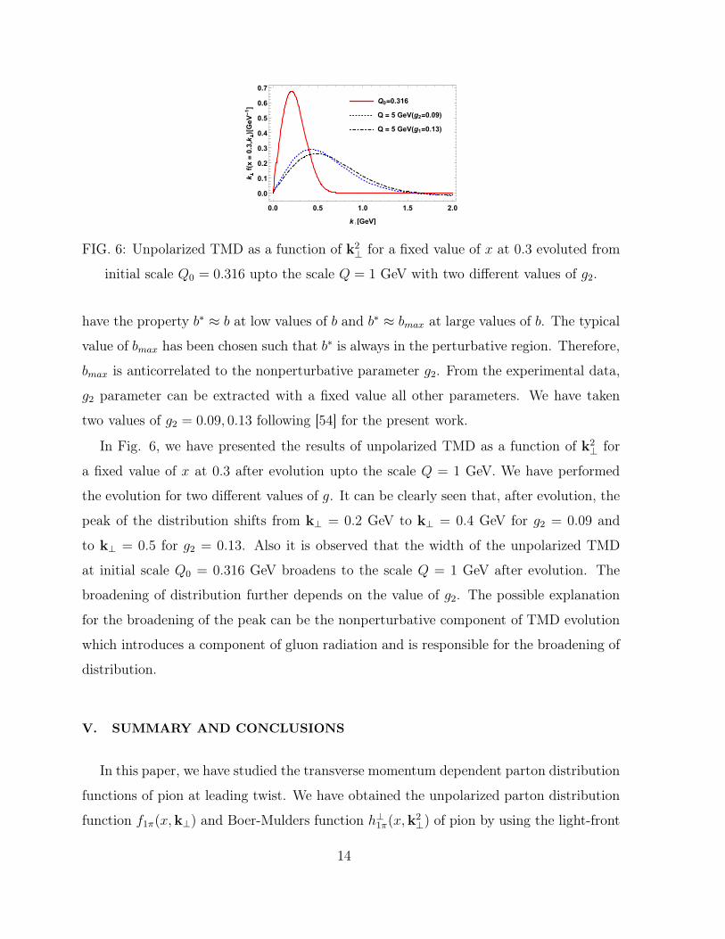
IV. EVOLUTION OF UNPOLARIZED TMD

The result of unpolarized TMD obtained in Eq. (13) is at a scale of 0.316 GeV. However,

to compare the present results with the future experimental data, the unpolarised TMD

needs to be evolved to higher scales. The evolution of TMD in the coordinate space (b⊥-

space) is comparatively more convenient than that in the momentum space (k⊥-space).

The pion TMD evolution from initial scale to another scale in the coordinate space (b⊥)

can be obtained using [71–74]

f1π(x, b⊥;µ) = expS(b∗;µb,µ) expgK(b⊥) ln µ

µ0 f1π(x, b⊥;µ0). (20)

Here, the Sudakov form factor S(b∗;µb, µ) is spin independent and is considered upto

next-to-leading logarithmic (NLL) approximation and at leading order in αs [75, 76].

The nonperturbative function gK(b⊥) in Eq. (20) is parametrized in quadratic form as

gK = −g2b2⊥/2 [77–79].

In the small b region, the b−dependent TMD is perturbatively calculable but in the

large b region, the dependence turns out to be nonperturbative. To obtain a complete

information of perturbative and nonperturbative part, a parameter bmax can be introduced

and we have

µb =C1

b∗(b⊥), b∗(b⊥) =

b⊥√

1 +b2⊥

b2max

. (21)

In the above expression, the constant C1 adopts a particular choice C1 = 2e−γE [71, 78],

where γE = 0.577 is the Euler constant [80]. A b−dependent function b∗ is defined to

13

Q0=0.316

Q = 5 GeV(g2=0.09)

Q = 5 GeV(g1=0.13)

0.0 0.5 1.0 1.5 2.0

0.0

0.1

0.2

0.3

0.4

0.5

0.6

0.7

k�[GeV]

k

�

f(x=0.3,k

�

)[GeV-1]

FIG. 6: Unpolarized TMD as a function of k2⊥ for a fixed value of x at 0.3 evoluted from

initial scale Q0 = 0.316 upto the scale Q = 1 GeV with two different values of g2.

have the property b∗ ≈ b at low values of b and b∗ ≈ bmax at large values of b. The typical

value of bmax has been chosen such that b∗ is always in the perturbative region. Therefore,

bmax is anticorrelated to the nonperturbative parameter g2. From the experimental data,

g2 parameter can be extracted with a fixed value all other parameters. We have taken

two values of g2 = 0.09, 0.13 following [54] for the present work.

In Fig. 6, we have presented the results of unpolarized TMD as a function of k2⊥ for

a fixed value of x at 0.3 after evolution upto the scale Q = 1 GeV. We have performed

the evolution for two different values of g. It can be clearly seen that, after evolution, the

peak of the distribution shifts from k⊥ = 0.2 GeV to k⊥ = 0.4 GeV for g2 = 0.09 and

to k⊥ = 0.5 for g2 = 0.13. Also it is observed that the width of the unpolarized TMD

at initial scale Q0 = 0.316 GeV broadens to the scale Q = 1 GeV after evolution. The

broadening of distribution further depends on the value of g2. The possible explanation

for the broadening of the peak can be the nonperturbative component of TMD evolution

which introduces a component of gluon radiation and is responsible for the broadening of

distribution.

V. SUMMARY AND CONCLUSIONS

In this paper, we have studied the transverse momentum dependent parton distribution

functions of pion at leading twist. We have obtained the unpolarized parton distribution

function f1π(x,k⊥) and Boer-Mulders function h⊥1π(x,k2⊥) of pion by using the light-front

14

holographic model with spin-improved wave functions. The result of f1π(x,k⊥) has been

compared with light-front constituent model and soft-wall AdS/QCD Model. The overall

nature of distribution is similar in all three models with little difference in their amplitude.

The amplitude of the distribution decreases with the increase in square of transverse

momentum k2⊥ for a fixed longitudinal momentum fraction x. The symmetric nature of

unpolarized quark distribution xf q1π(x,k

2⊥) of pion under the exchange of x −→ 1 − x

leads to a double peak of the distribution. The width of distribution peak is narrower

in our model as compared to distribution in LFCM and soft wall AdS/QCD model for a

fixed transverse momentum k2⊥ which show that the probability of finding the partons is

more in this region. Further, it is observed that the distribution is model independent

when the transverse momentum carried by the quarks is large.

The results for h⊥1π(x,k2⊥) have been calculated from the correlator function with Wilson

line. It is found that the probability of finding the quarks with transverse spin inside the

pion is less when they carry large transverse momentum. At smaller values of k2⊥, a

double peak is observed similar to the case of unpolarized quark distribution. The results

are compared with the light-front constituent model. At smaller values of transverse

momentum, the amplitudes of distribution in both models are different but at larger

values of transverse momentum results they agree quite well. In 0 ≤ k2⊥ ≤ 0.1 region, the

distribution in LFCM falls off rapidly with k2⊥ as compared to the case in our model.

From the results for positivity at different values of x it is observed that the amplitude

of h⊥1π(x,k2⊥) is smaller than the f1π(x,k⊥) and the inequality is very well satisfied even

at a large value of transverse momentum k⊥. The amplitude of unpolarized TMD is

always greater than the amplitude of Boer-Mulders function implying that the probability

of finding an unpolarized quark inside the pion is larger than the probability of the

finding transversely polarized quark in the pion. We have also performed the evolution of

f1π(x,k⊥) from initial model scale to higher scale. We have observed a width broadening

of distribution for evolution from initial scale Q0 = 0.316 GeV to the scale Q = 1 GeV.

The broadening of distribution depends on the value of nonperturbative parameter g2

which introduces a component of gluon radiation.

15

ACKNOWLEDGMENTS

H.D. would like to thank the Department of Science and Technology (Ref No.

EMR/2017/001549) Government of India for financial support.

[1] M. Burkardt, Phys. Rev. D 62, 071503 (2000); M. Burkardt, Phys. Rev. D 66, 119903

(2002).

[2] X. Ji, Phys. Rev. D 55, 7114 (1997).

[3] X. Ji, Phys. Rev. Lett. 78, 610 (1997).

[4] A. V. Radyushkin, Phys. Rev. D 56, 5524 (1997).

[5] X. Ji and J. Osborne, Phys, Rev. D 58, 094018 (1998).

[6] X. Ji, J. Phys. G: Nucl. Part Phys. 24, 1181 (1998).

[7] J. Blumlein, B. Geyer and D. Robaschik, Nucl. Phys. B 560, 283 (1999).

[8] K. Goeke, M. V. Polyakov, M. Vanderhaeghen, Progr. Part. Nucl. Phys. 47, 401 (2001).

[9] M. Diehl, Phys. Rep. 388, 41 (2003).

[10] R. D. Tangerman and P. J. Mulders, Phys. Rev. D 51, 3357 (1995).

[11] A. Kotzinian, Nucl. Phys. B 441, 234 (1995).

[12] P. J. Mulders and R. D. Tangerman, Nucl. Phys. B 461, 197 (1996); P. J. Mulders and R.

D. Tangerman, Nucl. Phys. B 484, 538 (1997).

[13] D. Boer and P. J. Mulders, Phys. Rev. D 57, 5780 (1998).

[14] A. Bacchetta, M. Diehl, K. Goeke, A. Metz, P. J. Mulders and M. Schlegel, JHEP 0702,

093 (2007).

[15] X. Ji, J. P. Ma and F. Yuan Phys. Rev. D 71, 034005 (2005).

[16] S. D. Drell and Tung-Mow Yan, Phys. Rev. Lett. 25, 316 (1970); S. D. Drell and Tung-Mow

Yan, Phys. Rev. Lett. 25,902(1970).

[17] J. H. Christenson et al., Phys. Rev. Lett. 25, 1523 (1970).

[18] J. C. Collins, Phys. Lett. B 536, 43 (2002).

[19] C. Quintans and the COMPASS Collaboration, J. of Phys. Conf. Ser. 295, 012163 (2011).

16

[20] S. P. Baranov, A. V. Lipatov and N. P. Zotov, Phys. Rev. D 89, 094025 (2014).

[21] D. Boer and P. J. Mulders, Phys. Rev. D 57, 5780 (1998).

[22] S. J. Brodsky, D. S. Hwang and I. Schmidt, Phys. Lett. B 530, 99 (2002).

[23] X. D. Ji and F. Yuan, Phys. Lett. B 543, 66 (2002).

[24] S. J. Brodsky, D. S. Hwang and I. Schmidt, Nucl. Phys. B 642, 344 (2002).

[25] D. Boer, S. J. Brodsky and D. S. Hwang, Phys. Rev. D 67, 054003 (2003).

[26] D. Boer, P. J. Mulders and F. Pijlman, Nucl. Phys. B 667, 201 (2003).

[27] A. V. Belitsky, X. Ji and F. Yuan, Nucl. Phys. B 656, 165 (2003).

[28] P. L. McGaughey, J. M. Moss and J. C. Peng, Ann. Rev. Nucl. Part. Sci. 49, 217 (1999).

[29] P. E. Reimer, J. Phys. G 34, S107 (2007).

[30] W. C. Chang and D. Dutta, Int. J. Mod. Phys. E 22, 1330020 (2013).

[31] J. C. Peng and J.-W. Qiu, Prog. Part. Nucl. Phys. 76, 43 (2014).

[32] G. Altarelli, S. Petrarca and F. Rapuano, Phys. Lett. B 373, 200 (1996).

[33] L. Chang, C. Mezrag, H. Moutarde, C. D. Roberts, J. R.-Quinterod and P. C. Tandy, Phys.

Lett. B 737, 23 (2014).

[34] C. Shi, C. Mezrag and H.-S. Zong, Phys. Rev. D 98, 054029 (2018)

[35] T. Nguyen, A. Bashir, C. D. Roberts and P. C. Tandy, Phys. Rev. C 83, 062201 (2011).

[36] L. Chang and A. W. Thomas, Phys. Lett. B, 749, 547-550 (2015).

[37] M. V. Polyakov and C. Weiss, Phys. Rev. D 60, 114017 (1999).

[38] S. Dalley, Phys. Rev. D 64, 036006 (2001).

[39] R. M. Davidson and E. R. Arriola, Acta. Phys. Polon. B 33, 1791 (2002).

[40] S. Dalley and B. V. Sande, Phys. Rev. D 67, 114507 (2003).

[41] W. Broniowski and E. R. Arriola, Phys. Lett. B 574, 57 (2003).

[42] D. Bromel et al., Phys. Rev. Lett. 101, 122001 (2008).

[43] T. Frederico, E. Pace, B. Pasquini and G. Salme, Phys. Rev D 80, 054021 (2009).

[44] A. E. Dorokhov, W. Broniowski and E. R. Arriola, Phys. Rev. D 84, 074015 (2011).

[45] C. Mezrag, L. Chang, H. Moutarde, C. D. Roberts, J. R.-Quintero , F. SabatiÃľ and S. M.

Schmidt, Phys. Lett. B 741, 190 (2015).

17

[46] T. Gutsche, V. E. Lyubovitskij, I. Schmidt and A. Vega, J. Phys. G: Nucl. Part. Phys. 42,

095005 (2015).

[47] B. Pasquini and P. Schweitzer, Phys. Rev. D 90, 014050 (2014).

[48] C. LorcÃľ, B. Pasquini and P. Schweitzer, Eur. Phys. J. C 76, 7, 415 (2016).

[49] Z. Lu and B. Q. Ma, Nucl. Phys. A 741, 200 (2004).

[50] S. Meissner, A. Metz, M. Schlegel and K. Goeke, J. High Energy Phys. 08, 038 (2008).

[51] L. Gamberg and M. Schlegel, Phys. Lett. B 685, 95 (2010)

[52] Z. Lua, B.-Q. Ma, Phys. Rev. D 70, 094044 (2004).

[53] S. Noguera and S. Scopetta, J. High Energy Phys. , 102 (2015)

[54] A. Bacchetta, S. Cotogno and B. Pasquini, Phys. Lett. B 771, 546-552 (2017).

[55] N. Kaur, N. Kumar, C. Mondal and H. Dahiya, Nucl. Phys. B 934, 80-95 (2018).

[56] G. F. de Teramond and S. J. Brodsky, Phys. Rev. Lett. 94, 201601 (2005).

[57] S. J. Brodsky and G. F. de Teramond, Phys. Rev. Lett. 96, 201601 (2006).

[58] G. F. de Teramond and S. J. Brodsky, Phys. Rev. Lett. 102, 081601 (2009).

[59] S. J. Brodsky, G. F. de Teramond and H. G. Dosch, Phys. Lett. B 729, 3(2014).

[60] S. J. Brodsky, G. F. de Teramond, H. G. Dosch and J. Erlich, Phys. Rept 584, 1 (2015).

[61] S. J. Brodsky and G. F. de Teramond, Subnucl. Ser. 45, 139 (2009).

[62] A. Vega and I. Schmidt, Phys. Rev. D 79, 055003 (2009).

[63] A. Vega, I. Schmidt, T. Branz, T. Gutsche and V. E. Lyubovitskij, Phys. Rev. D 80, 055014

(2009).

[64] R. Swarnkar and D. Chakrabarti, Phys. Rev. D 92, 074023 (2015).

[65] M. Ahmady, F. Chishtie and R. Sandapen, Phys. Rev. D 95, 074008, (2017).

[66] M. Ahmady, C. Mondal and R. Sandapen, Phys. Rev. D 98, 034010 (2018).

[67] B. Pasquini and F. Yuan, Phys. Rev. D 81, 114013 (2010).

[68] B. Pasquini and P. Schweitzer, Phys. Rev. D 78, 071502 (2008).

[69] S. Meissner, A. Metz and K. Goeke, Phys. Rev. D 76, 034002 (2007).

[70] Z. Lua and B.-Q. Ma, Phys. Lett. B 615, 200âĂŞ206 (2005).

[71] S. M. Aybat and T. C. Rogers, Phys. Rev. D 83, 114042 (2011).

18

[72] J. Collins, Cambridge Monographs on Particle Physics, Nuclear Physics and Cosmology, 32

Cambridge University Press (2011).

[73] T. C. Rogers, Eur. Phys. J. A 52 (6), 153 (2016).

[74] J. Collins and T. Rogers, Phys. Rev. D 91, 074020, (2015).

[75] S. Frixione, P. Nason and G. Ridolfi, Nucl. Phys. B 542, 311 (1999).

[76] M. G. Echevarria, A. Idilbi, A. SchÃďfer and I. Scimemi, Eur. Phys. J. C 73(12), 2636

(2013).

[77] M. Anselmino, M. Boglione and S. Melis, Phys. Rev. D 86, 014028 (2012).

[78] S. M. Aybat, J. C. Collins, J. W. Qiu and T. C. Rogers, Phys. Rev. D 85, 034043 (2012).

[79] F. Landry, R. Brock, P. M. Nadolsky and C. P. Yuan, Phys. Rev. D 67, 073016 (2003).

[80] J. C. Collins, D. E. Soper and G. F. Sterman, Nucl. Phys. B 250, 199 (1985).

19