Data Structures

Sorting in Linear Time

1

Sorting

• Internal (external) – All data are held in primary memory during the

sorting process. • Comparison Based

– Based on pairwise comparisons. – Lower bound on running time is Ω(nlogn).

• In Place – Requires very little, O(log n), additional space.

• Stable – Preserves the relative ordering of items with equal

values.

2

• Ω(n) to examine all the input.

• All sorts seen so far are Ω(n lg n).

• We’ll show that Ω(n lg n) is a lower bound for comparison sorts.

Lower Bounds for Comparison Sorts

3

Lower Bounds for Comparison Sorts

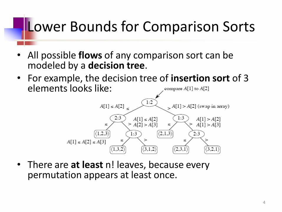
• All possible flows of any comparison sort can be modeled by a decision tree.

• For example, the decision tree of insertion sort of 3 elements looks like:

• There are at least n! leaves, because every permutation appears at least once.

4

Lower Bounds for Comparison Sorts

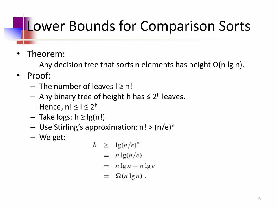
• Theorem: – Any decision tree that sorts n elements has height Ω(n lg n).

• Proof: – The number of leaves l ≥ n! – Any binary tree of height h has ≤ 2h leaves. – Hence, n! ≤ l ≤ 2h – Take logs: h ≥ lg(n!) – Use Stirling’s approximation: n! > (n/e)n

– We get:

5

Lower Bounds for Comparison Sorts

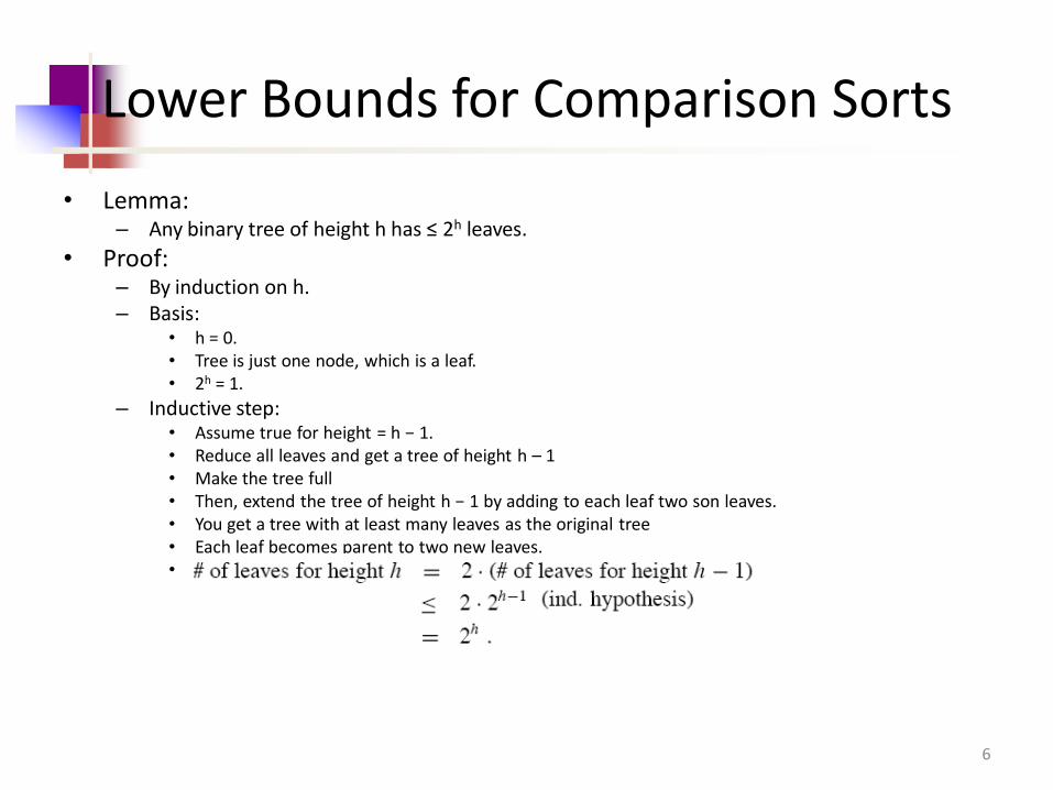
• Lemma: – Any binary tree of height h has ≤ 2h leaves.

• Proof: – By induction on h. – Basis:

• h = 0. • Tree is just one node, which is a leaf. • 2h = 1.

– Inductive step: • Assume true for height = h − 1. • Reduce all leaves and get a tree of height h – 1 • Make the tree full • Then, extend the tree of height h − 1 by adding to each leaf two son leaves. • You get a tree with at least many leaves as the original tree • Each leaf becomes parent to two new leaves. •

6

Sorting in Linear Time

• Non-comparison sorts.

• Counting Sort

• Radix Sort

• Bucket Sort

7

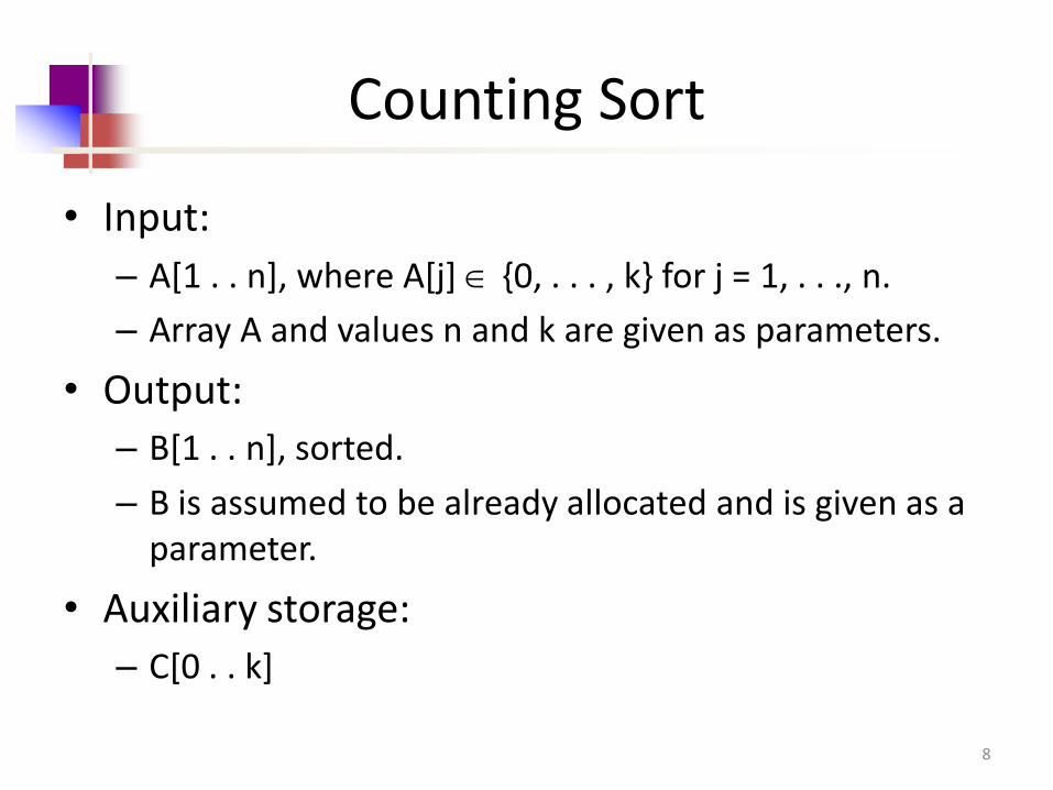
Counting Sort

• Input:

– A[1 . . n], where A[j] {0, . . . , k} for j = 1, . . ., n.

– Array A and values n and k are given as parameters.

• Output:

– B[1 . . n], sorted.

– B is assumed to be already allocated and is given as a parameter.

• Auxiliary storage:

– C[0 . . k]

8

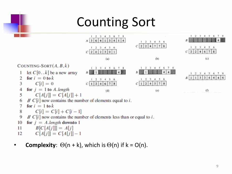
Counting Sort

• Complexity: (n + k), which is (n) if k = O(n).

9

Counting Sort

• How big a k is practical?

– 32-bit values? No.

– 16-bit? Probably not.

– 8-bit? Maybe, depending on n.

– 4-bit? Yes (unless n is really small).

10

Counting Sort

• Counting sort is stable

– Keys with same value appear in same order in output as they did in input

– Because of how the last loop works.

11

Radix Sort

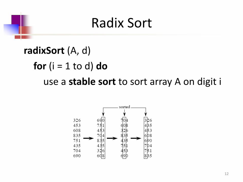
radixSort (A, d)

for (i = 1 to d) do

use a stable sort to sort array A on digit i

12

Radix Sort

• Complexity:

– Assume that we use counting sort as the intermediate sort.

– (n + k) per pass (digits in range 0, . . . , k).

– d passes.

– (d(n + k)) total.

– If k = O(n), time = (dn).

13

Radix Sort

• Notations: – n words. – b bits/word. – Break into r-bit digits.

• Have d = b/r.

– Use counting sort, k = 2r. – Example:

• 32-bit words, 8-bit digits. • b = 32, r = 8, d = 32/8 = 4, k = 28 = 256.

• Complexity: – ((b/r)·(n + 2r)).

14

Radix Sort

• How to choose r? – Balance b/r and n + 2r.

– Choosing r ≈ lg n gives us (b/lgn (n + n)) = ((b/lgn)·n). – If we choose r < lg n, then

• b/r > b/ lg n, and n + 2r term doesn’t improve.

– If we choose r > lg n, then • n + 2r term gets big. • For instance: r = 2 lg n 2r = 22 lgn = (2lg n)2 = n2.

• Example: – To sort 216 32-bit numbers, – Use r = lg 216 = 16 bits. – Get b/r = 2 passes.

15

Radix Sort

• Compare radix sort to merge and quicksort:

– 1 million (220) 32-bit integers.

– Radix sort: 32/20 = 2 passes.

– Merge sort/quicksort: lg n = 20 passes.

• Remember, though, that each radix sort “pass” is really 2 passes

– one to take census, and one to move data.

16

Radix Sort

• Not a comparison sort:

– We gain information about keys by means other than direct comparison of two keys.

– Use keys as array indices.

17

Bucket Sort

• Assumes the input is – Generated by a random process that distributes

elements uniformly over [0, 1).

• Then – Divide [0, 1) into n equal-sized buckets.

– Distribute the n input values into the buckets.

– Sort each bucket.

– Go through buckets in order, listing elements in each one.

18

Bucket Sort

• Input:

– A[1 . . n], where 0 ≤ A[i] < 1 for all i .

• Auxiliary array:

– B[0 . . n − 1] of linked lists, each list initially empty.

19

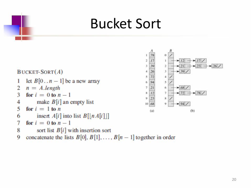
Bucket Sort

20

Bucket Sort

• Complexity:

– All lines of algorithm except insertion sorting take (n) altogether.

– If each bucket gets O(1) elements, the time to sort all buckets is O(n).

– Hence, (n) altogether.

• Formally …

21

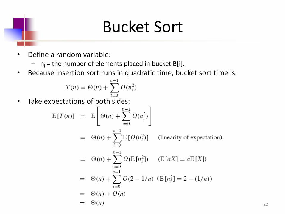
• Define a random variable: – ni = the number of elements placed in bucket B[i].

• Because insertion sort runs in quadratic time, bucket sort time is:

• Take expectations of both sides:

Bucket Sort

22

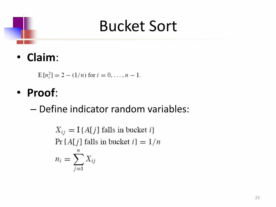
Bucket Sort

• Claim:

• Proof:

– Define indicator random variables:

23

Bucket Sort

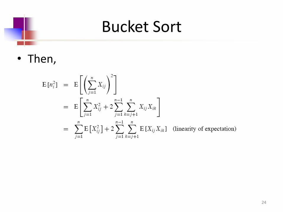
• Then,

24

Bucket Sort

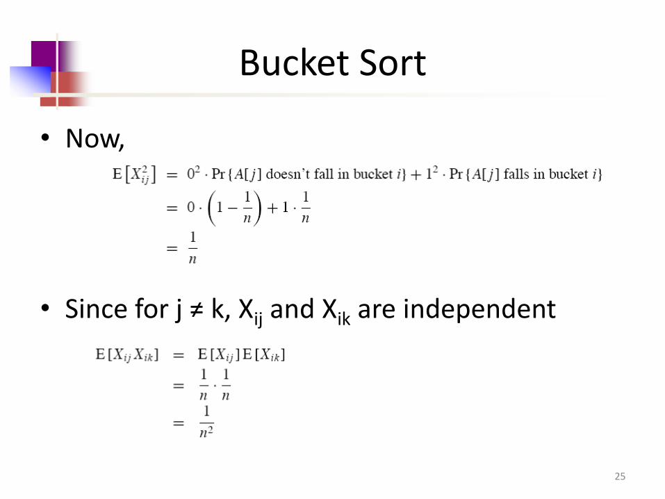
• Now,

• Since for j ≠ k, Xij and Xik are independent

25

Bucket Sort

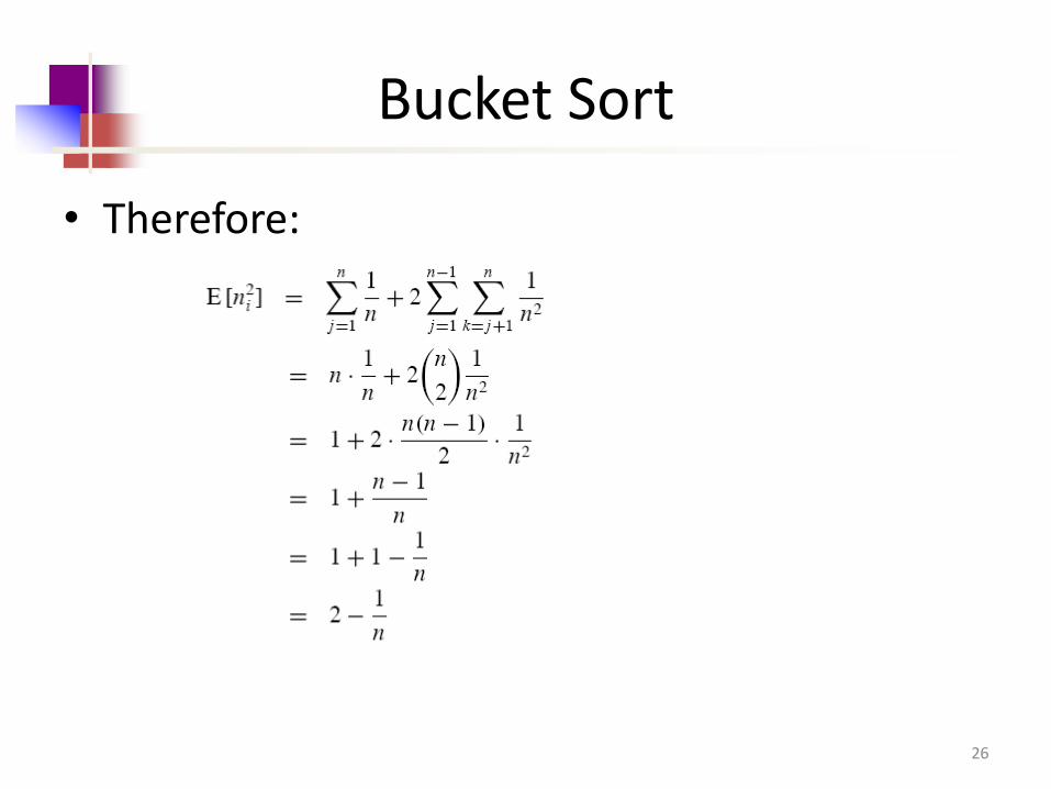
• Therefore:

26

Bucket Sort

• Again, not a comparison sort. – Used a function of key values to index into an array.

• This is a probabilistic analysis. – We used probability to analyze an algorithm whose

running time depends on the distribution of inputs.

• Different from a randomized algorithm, where – We use randomization to impose a distribution.

• If the input isn’t drawn from a uniform distribution on [0, 1), – All bets are off, but the algorithm is still correct.

27