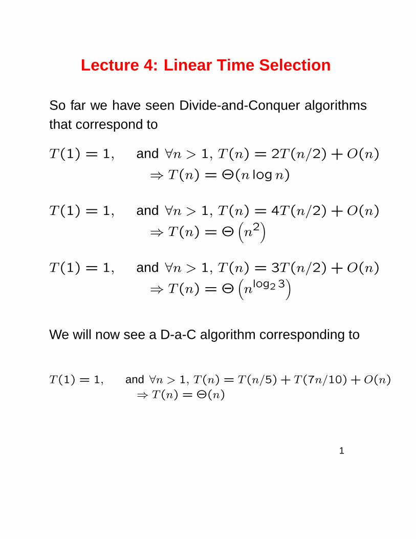
Lecture 4: Linear Time Selection

So far we have seen Divide-and-Conquer algorithmsthat correspond to

T (1) = 1, and ∀n > 1, T (n) = 2T (n/2) + O(n)

⇒ T (n) = Θ(n logn)

T (1) = 1, and ∀n > 1, T (n) = 4T (n/2) + O(n)

⇒ T (n) = Θ(

n2)

T (1) = 1, and ∀n > 1, T (n) = 3T (n/2) + O(n)

⇒ T (n) = Θ(

nlog2 3)

We will now see a D-a-C algorithm corresponding to

T(1) = 1, and ∀n > 1, T(n) = T(n/5) + T(7n/10) + O(n)

⇒ T(n) = Θ(n)

1

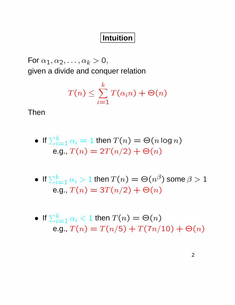
Intuition

For α1, α2, . . . , αk > 0,

given a divide and conquer relation

T (n) ≤k

∑

i=1

T (αin) + Θ(n)

Then

• If∑k

i=1 αi = 1 then T (n) = Θ(n logn)

e.g., T (n) = 2T (n/2) + Θ(n)

• If∑k

i=1 αi > 1 then T (n) = Θ(nβ) some β > 1

e.g., T (n) = 3T (n/2) + Θ(n)

• If∑k

i=1 αi < 1 then T (n) = Θ(n)

e.g., T (n) = T (n/5) + T (7n/10) + Θ(n)

2

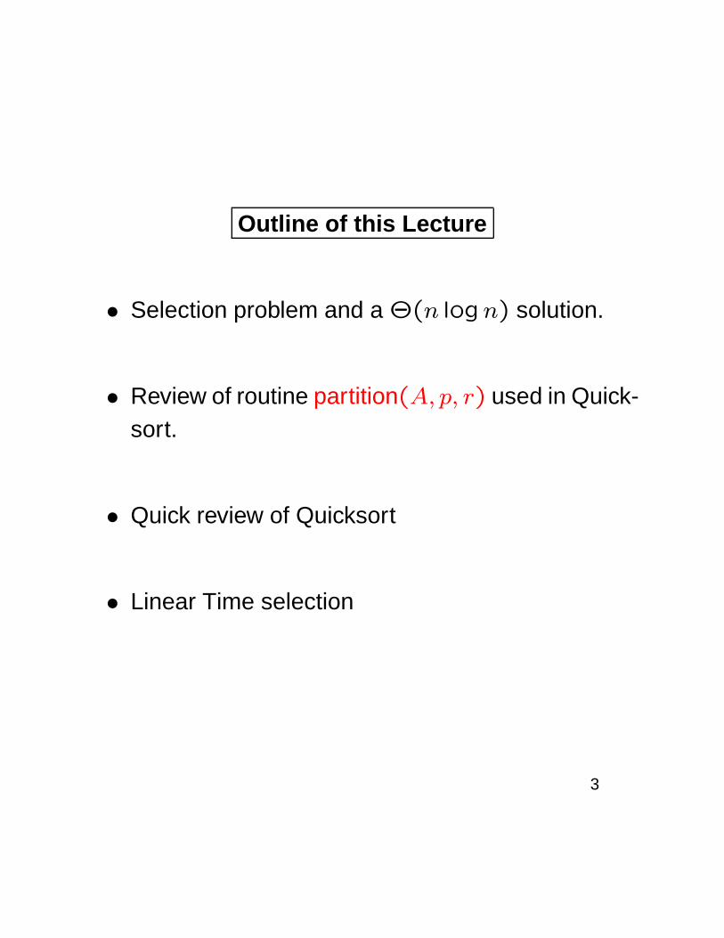
Outline of this Lecture

• Selection problem and a Θ(n logn) solution.

• Review of routine partition(A, p, r) used in Quick-sort.

• Quick review of Quicksort

• Linear Time selection

3

Readings

• Quicksort and Partition:CLRS, pages 144-53.

• Linear Time Selection:CLRS, pages 185-195.

• Review of Divide and conquer recurrences (andthe master method for solving them):CLRS, Chapter 4.

4

The Selection Problem

Sel(A, i) :

Given a sequence of numbers 〈a1, . . . , an〉, and aninteger i, 1 ≤ i ≤ n, find the ith smallest element.When i = dn/2e, this is called the median problem.

Example: Given 〈1,8,23,10,19,33,100〉, the 4thsmallest element is 19.

Question: How do you solve this problem?

5

First Solution: Selection by Sorting

Step 1: Sort the elements in ascending order with anyalgorithm of complexity O(n logn).

Step 2: Return the ith element of the sorted array.

The complexity of this solution is Θ(n logn).

Question: Can we do better?

Answer: YES, but we need to recall Partition(A, p, r)used in Quicksort!

6

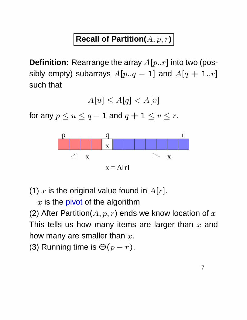
Recall of Partition(A, p, r)

Definition: Rearrange the array A[p..r] into two (pos-sibly empty) subarrays A[p..q − 1] and A[q + 1..r]

such that

A[u] ≤ A[q] < A[v]

for any p ≤ u ≤ q − 1 and q + 1 ≤ v ≤ r.

x

p rq

x x

x = A[r]

(1) x is the original value found in A[r].

x is the pivot of the algorithm(2) After Partition(A, p, r) ends we know location of x

This tells us how many items are larger than x andhow many are smaller than x.(3) Running time is Θ(p− r).

7

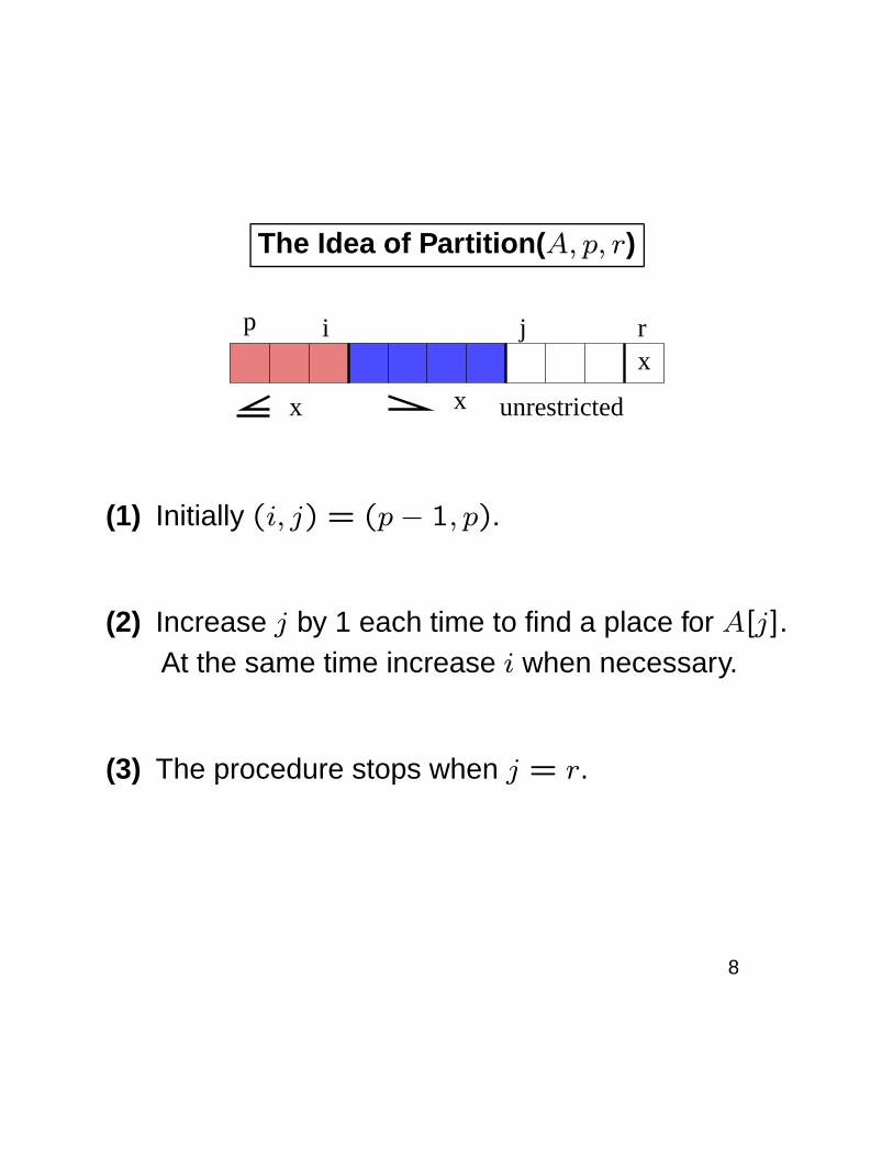
The Idea of Partition(A, p, r)

ip j rx

x x unrestricted

(1) Initially (i, j) = (p− 1, p).

(2) Increase j by 1 each time to find a place for A[j].At the same time increase i when necessary.

(3) The procedure stops when j = r.

8

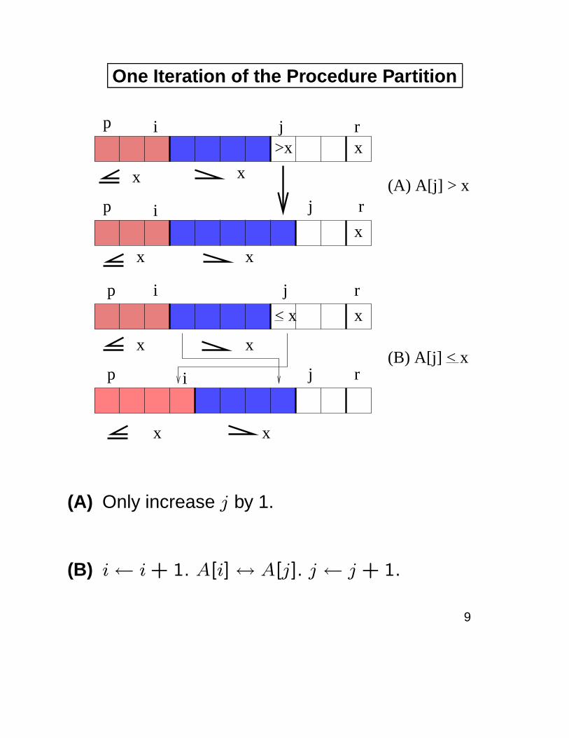
One Iteration of the Procedure Partition

ip j rx

x x

>x

jp i

x x

x

r

rp

x x

i j

x< x

p i j r

x x

(A) A[j] > x

(B) A[j] < x

(A) Only increase j by 1.

(B) i← i + 1. A[i]↔ A[j]. j ← j + 1.

9

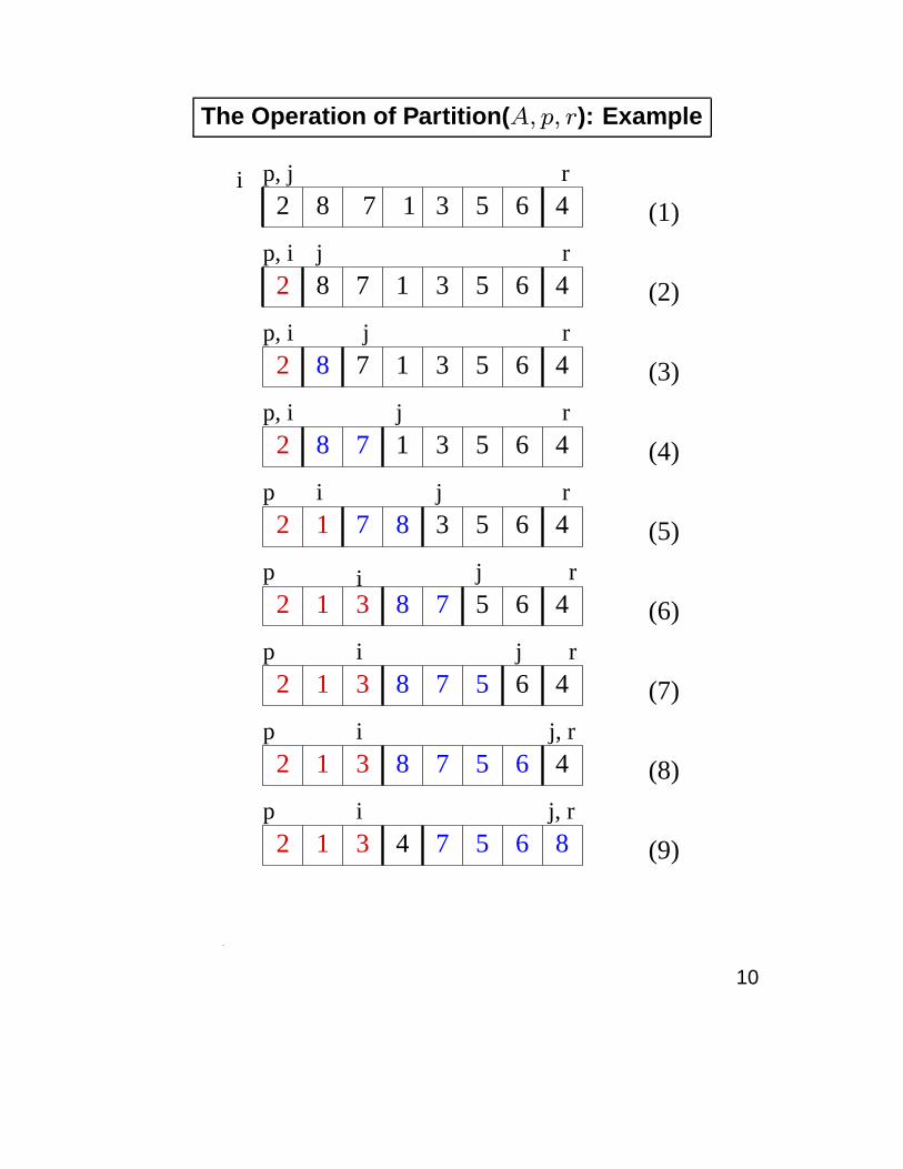
The Operation of Partition(A, p, r): Example

i

j

j

j

p i j

p i j

p i j

p i j, r

p i j, r

r

r

r

r

r

r

rp, j

p, i

p, i

p, i

2 8 7 41 3 5 6

2

2

2

2

2

2

2

2

1

1

1

1

1 3

3

3

3

8

8

8

8

8

8

8

7

7

7

7

7

7

5

5

5

6

6

8 7 1 3 5 6 4

7 1 3 5 6 4

1 3 5 6 4

3 5 6 4

5 6 4

6 4

4

4

(1)

(2)

(3)

(4)

(5)

(6)

(9)

(7)

(8)

10

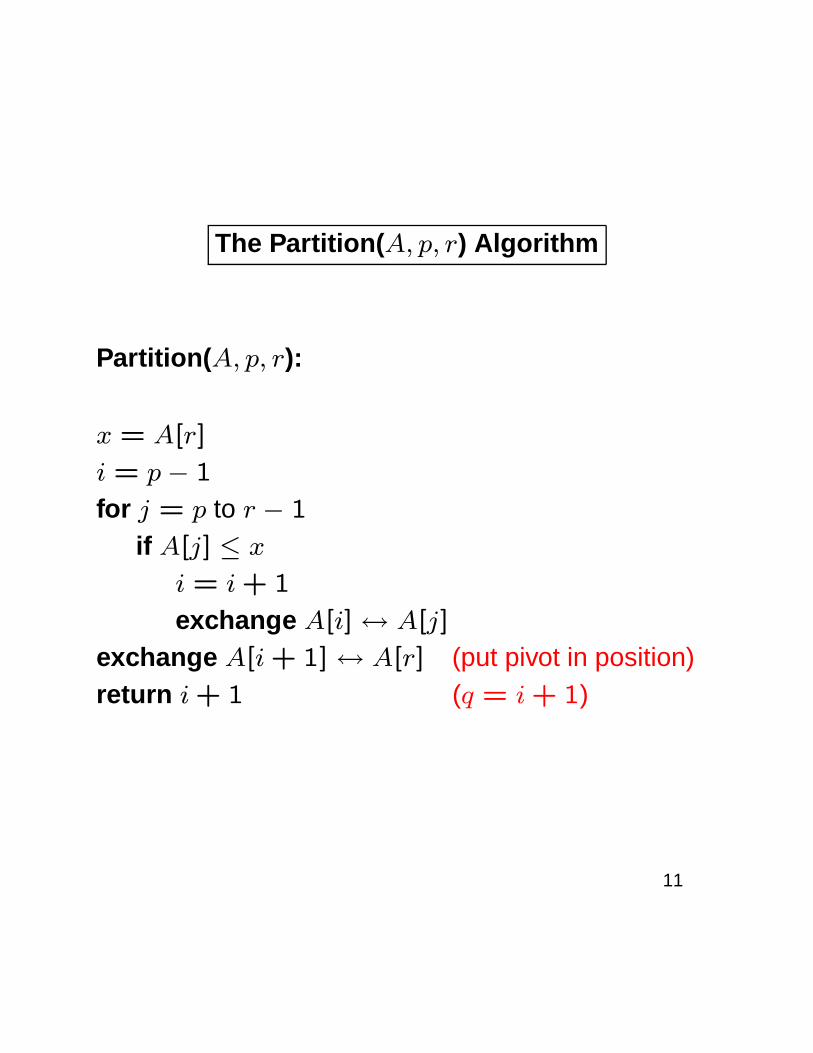
The Partition(A, p, r) Algorithm

Partition(A, p, r):

x = A[r]

i = p− 1

for j = p to r − 1

if A[j] ≤ x

i = i + 1

exchange A[i]↔ A[j]

exchange A[i + 1]↔ A[r] (put pivot in position)return i + 1 (q = i + 1)

11

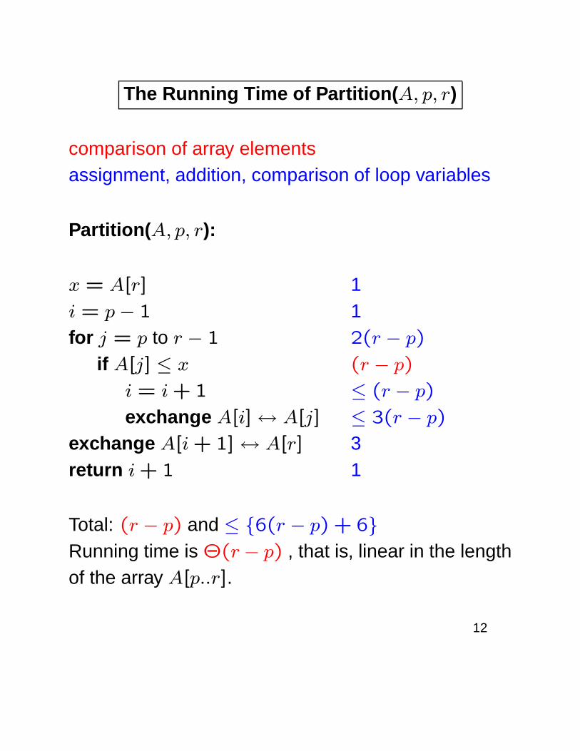
The Running Time of Partition(A, p, r)

comparison of array elementsassignment, addition, comparison of loop variables

Partition(A, p, r):

x = A[r] 1i = p− 1 1for j = p to r − 1 2(r − p)

if A[j] ≤ x (r − p)

i = i + 1 ≤ (r − p)

exchange A[i]↔ A[j] ≤ 3(r − p)

exchange A[i + 1]↔ A[r] 3return i + 1 1

Total: (r − p) and ≤ {6(r − p) + 6}

Running time is Θ(r− p) , that is, linear in the lengthof the array A[p..r].

12

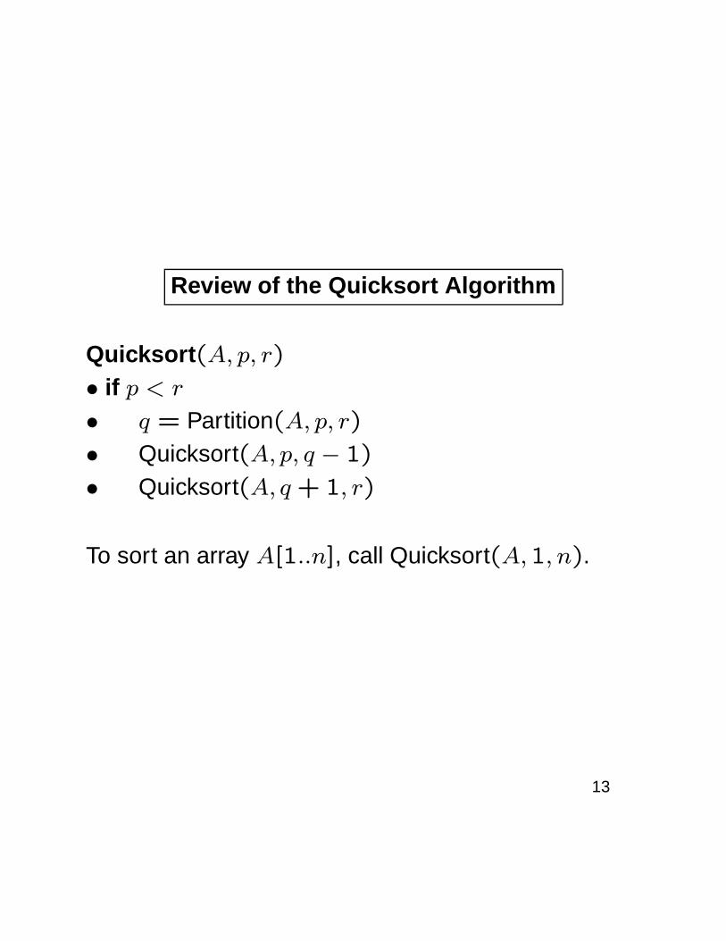
Review of the Quicksort Algorithm

Quicksort(A, p, r)

• if p < r

• q = Partition(A, p, r)

• Quicksort(A,p, q − 1)

• Quicksort(A, q + 1, r)

To sort an array A[1..n], call Quicksort(A,1, n).

13

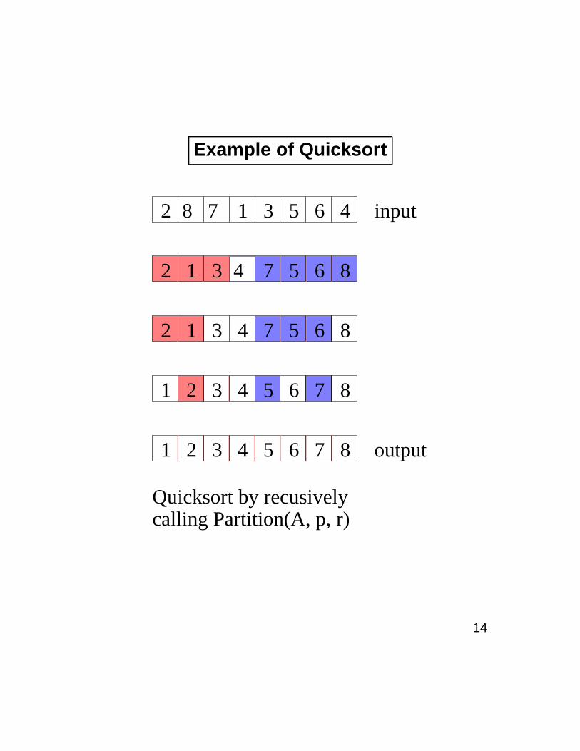
Example of Quicksort

2 8 7 1 3 5 6 4

2 1 3 4 7 5 6 8

3 4 82 1 7 5 6

1 2 3 4 65 7 8

1 2 3 4 5 6 7 8

Quicksort by recusively calling Partition(A, p, r)

output

input

14

Running Time of Quicksort

Worst Case: T (n) = Θ(n2).

Average Case: T (n) = O(n logn).

Remark: This is a review only and we do not give therunning time analysis.

Exercise: Let Q(n) denote the average number ofcomparisons of array elements done by the Quicksortalgorithm.Explain why

Q(n) = n− 1 +1

n

n∑

k=1

{Q(n− k) + Q(k − 1)}.

Show that

Q(n) = 2(n + 1)Hn − 4n.

15

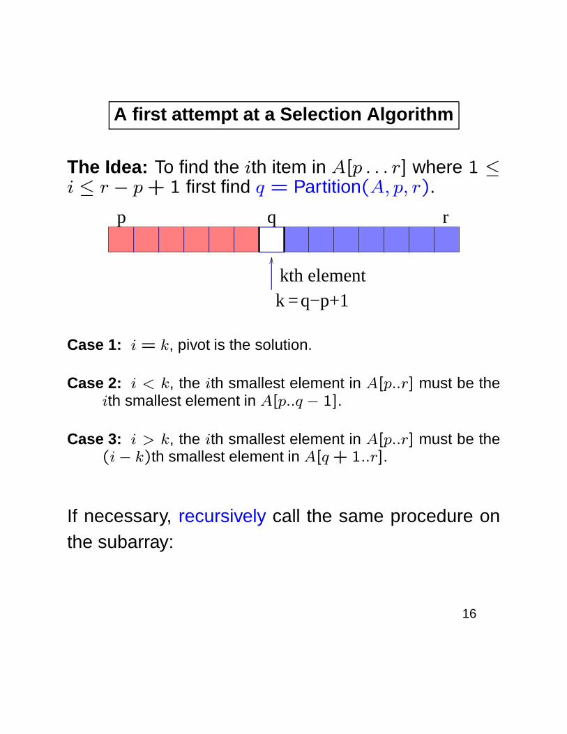
A first attempt at a Selection Algorithm

The Idea: To find the ith item in A[p . . . r] where 1 ≤i ≤ r − p + 1 first find q = Partition(A, p, r).

p q r

k =kth element

q−p+1

Case 1: i = k, pivot is the solution.

Case 2: i < k, the ith smallest element in A[p..r] must be theith smallest element in A[p..q − 1].

Case 3: i > k, the ith smallest element in A[p..r] must be the(i− k)th smallest element in A[q + 1..r].

If necessary, recursively call the same procedure onthe subarray:

16

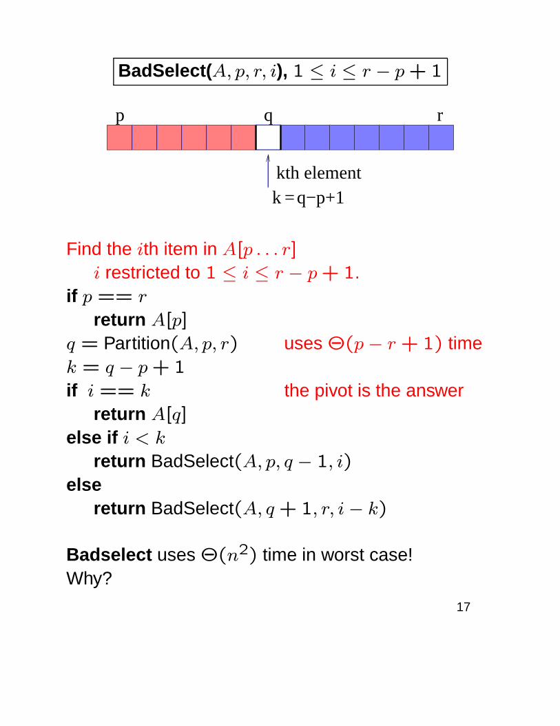
BadSelect(A, p, r, i), 1 ≤ i ≤ r − p + 1

p q r

k =kth element

q−p+1

Find the ith item in A[p . . . r]

i restricted to 1 ≤ i ≤ r − p + 1.if p == r

return A[p]

q = Partition(A, p, r) uses Θ(p− r + 1) timek = q − p + 1

if i == k the pivot is the answerreturn A[q]

else if i < k

return BadSelect(A, p, q − 1, i)

elsereturn BadSelect(A, q + 1, r, i− k)

Badselect uses Θ(n2) time in worst case!Why?

17

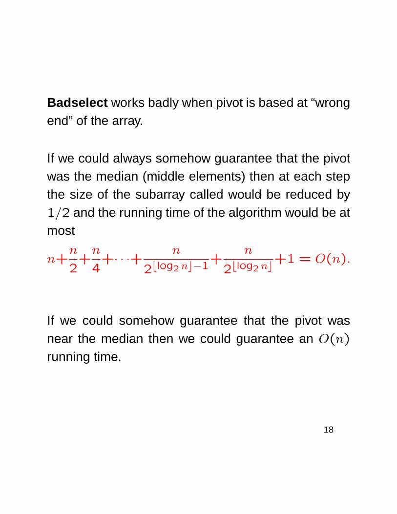
Badselect works badly when pivot is based at “wrongend” of the array.

If we could always somehow guarantee that the pivotwas the median (middle elements) then at each stepthe size of the subarray called would be reduced by1/2 and the running time of the algorithm would be atmost

n+n

2+

n

4+· · ·+

n

2blog2 nc−1+

n

2blog2 nc+1 = O(n).

If we could somehow guarantee that the pivot wasnear the median then we could guarantee an O(n)

running time.

18

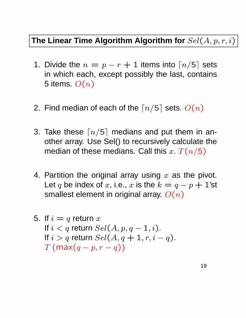
The Linear Time Algorithm Algorithm for Sel(A, p, r, i)

1. Divide the n = p − r + 1 items into dn/5e setsin which each, except possibly the last, contains5 items. O(n)

2. Find median of each of the dn/5e sets. O(n)

3. Take these dn/5e medians and put them in an-other array. Use Sel() to recursively calculate themedian of these medians. Call this x. T (n/5)

4. Partition the original array using x as the pivot.Let q be index of x, i.e., x is the k = q − p + 1’stsmallest element in original array. O(n)

5. If i = q return xIf i < q return Sel(A, p, q − 1, i).If i > q return Sel(A, q + 1, r, i− q).T (max(q − p, r − q))

19

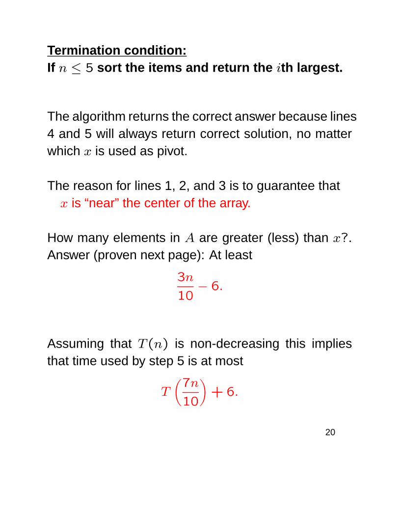
Termination condition:If n ≤ 5 sort the items and return the ith largest.

The algorithm returns the correct answer because lines4 and 5 will always return correct solution, no matterwhich x is used as pivot.

The reason for lines 1, 2, and 3 is to guarantee thatx is “near” the center of the array.

How many elements in A are greater (less) than x?.Answer (proven next page): At least

3n

10− 6.

Assuming that T (n) is non-decreasing this impliesthat time used by step 5 is at most

T

(

7n

10

)

+ 6.

20

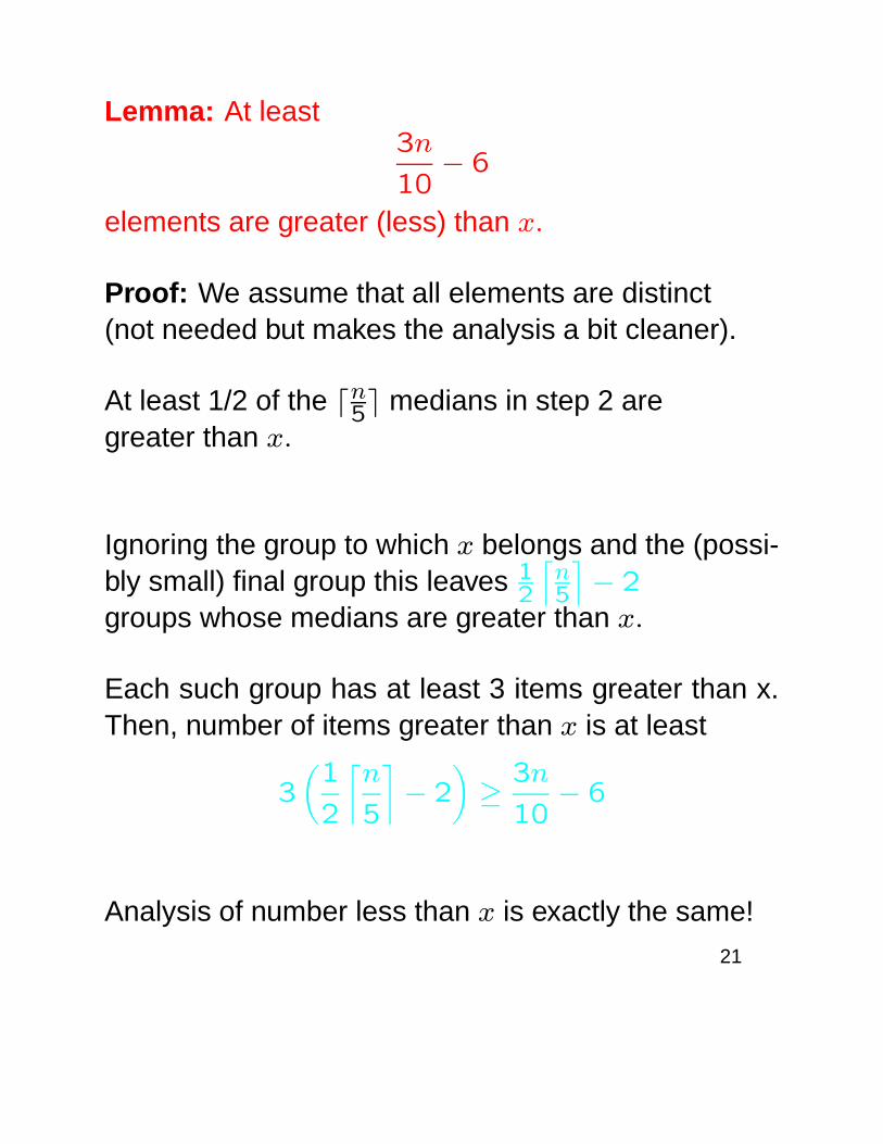
Lemma: At least3n

10− 6

elements are greater (less) than x.

Proof: We assume that all elements are distinct(not needed but makes the analysis a bit cleaner).

At least 1/2 of the dn5e medians in step 2 aregreater than x.

Ignoring the group to which x belongs and the (possi-bly small) final group this leaves 1

2

⌈

n5

⌉

− 2

groups whose medians are greater than x.

Each such group has at least 3 items greater than x.Then, number of items greater than x is at least

3

(

1

2

⌈

n

5

⌉

− 2

)

≥3n

10− 6

Analysis of number less than x is exactly the same!

21

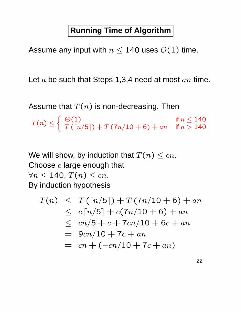
Running Time of Algorithm

Assume any input with n ≤ 140 uses O(1) time.

Let a be such that Steps 1,3,4 need at most an time.

Assume that T (n) is non-decreasing. Then

T(n) ≤

{

Θ(1) if n ≤ 140T (dn/5e) + T (7n/10 + 6) + an if n > 140

We will show, by induction that T (n) ≤ cn.Choose c large enough that∀n ≤ 140, T (n) ≤ cn.

By induction hypothesis

T (n) ≤ T (dn/5e) + T (7n/10 + 6) + an

≤ c dn/5e+ c(7n/10 + 6) + an

≤ cn/5 + c + 7cn/10 + 6c + an

= 9cn/10 + 7c + an

= cn + (−cn/10 + 7c + an)

22

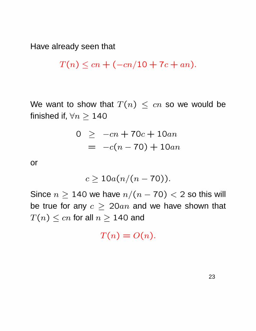
Have already seen that

T (n) ≤ cn + (−cn/10 + 7c + an).

We want to show that T (n) ≤ cn so we would befinished if, ∀n ≥ 140

0 ≥ −cn + 70c + 10an

= −c(n− 70) + 10an

or

c ≥ 10a(n/(n− 70)).

Since n ≥ 140 we have n/(n− 70) < 2 so this willbe true for any c ≥ 20an and we have shown thatT (n) ≤ cn for all n ≥ 140 and

T (n) = O(n).

23

Review

In this lecture we have

• Reviewed partition and quicksort.

• Reviewed different cases of divide-and-conquerrecurrences

• Derived a linear time selection algorithm.

Note: In practice, the constant in the O(n) runningtime of our selection algorithm is rather high so peopleuse the randomized selection algorithm described onpages 185-89 of CLRS.

24

Review of Divide-and-Conquer

In this section we have learnt how to apply the tech-nique of divide-and-conquer to design of efficient al-gorithms.

In the simplest version of D-a-C, e.g., maximum con-tiguous subarray, mergesort, the algorithm partitionsthe data into (almost) equal sized subinstances, solvesthe problem on the subinstances, and then combinesthose solutions together.

In some more advanced cases, e.g., polynomial mul-tiplication, the idea is not to partition the data but tocreate smaller (usually almost equal) sized subprob-lems that are solved.

In even more advanced cases, e.g., selection, the ideais to observe that the problem can be solved if we areable to solve smaller sized-subproblems. These sub-problems might no longer be found by simple data-splitting, though.

25