Data Compression TechniquesPart 1: Entropy Coding

Lecture 3: Entropy and Arithmetic Coding

Juha Karkkainen

07.11.2017

1 / 24

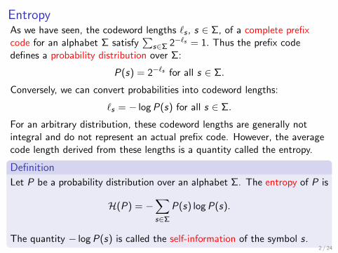
EntropyAs we have seen, the codeword lengths `s , s ∈ Σ, of a complete prefixcode for an alphabet Σ satisfy

∑s∈Σ 2−`s = 1. Thus the prefix code

defines a probability distribution over Σ:

P(s) = 2−`s for all s ∈ Σ.

Conversely, we can convert probabilities into codeword lengths:

`s = − log P(s) for all s ∈ Σ.

For an arbitrary distribution, these codeword lengths are generally notintegral and do not represent an actual prefix code. However, the averagecode length derived from these lengths is a quantity called the entropy.

Definition

Let P be a probability distribution over an alphabet Σ. The entropy of P is

H(P) = −∑s∈Σ

P(s) log P(s).

The quantity − log P(s) is called the self-information of the symbol s.2 / 24

The concept of (information theoretic) entropy was introduced in 1948 byClaude Shannon in his paper “A Mathematical Theory of Communication”that established the discipline of information theory. From that paper isalso the following result.

Theorem (Noiseless Coding Theorem)

Let C be an optimal prefix code for an alphabet Σ with the probabilitydistribution P. Then

H(P) ≤∑s∈Σ

P(s)|C (s)| < H(P) + 1.

The same paper contains the Noisy-channel Coding Theorem that dealswith coding in the presence of error.

3 / 24

The entropy is an absolute lower bound on compressibility in the averagesense. Because of integral code lengths, a prefix codes may not quitematch the lower bound, but the upper bound shows that they can getfairly close.

Example

symbol a e i o u yprobability 0.2 0.3 0.1 0.2 0.1 0.1

self-information 2.32 1.74 3.32 2.32 3.32 3.32Huffman codeword length 2 2 3 2 4 4

H(P) ≈ 2.45 while the average Huffman code length is 2.5.

We will later see how to get even closer to entropy, but it is never possibleto get below.

We will next prove the Noiceless Coding Theorem, and for that we willneed Gibbs’ Inequality.

4 / 24

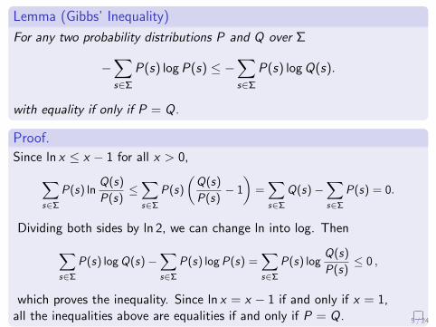
Lemma (Gibbs’ Inequality)

For any two probability distributions P and Q over Σ

−∑s∈Σ

P(s) log P(s) ≤ −∑s∈Σ

P(s) log Q(s).

with equality if only if P = Q.

Proof.

Since ln x ≤ x − 1 for all x > 0,∑s∈Σ

P(s) lnQ(s)

P(s)≤∑s∈Σ

P(s)

(Q(s)

P(s)− 1

)=∑s∈Σ

Q(s)−∑s∈Σ

P(s) = 0.

Dividing both sides by ln 2, we can change ln into log. Then∑s∈Σ

P(s) log Q(s)−∑s∈Σ

P(s) log P(s) =∑s∈Σ

P(s) logQ(s)

P(s)≤ 0 ,

which proves the inequality. Since ln x = x − 1 if and only if x = 1,all the inequalities above are equalities if and only if P = Q. 5 / 24

Proof of Noiseless Coding TheoremLet us prove the upper bound first. For all s ∈ Σ, let `s = d− log P(s)e.Then ∑

s∈Σ

2−`s ≤∑s∈Σ

2log P(s) =∑s∈Σ

P(s) = 1

and by Kraft’s inequality, there exists a (possibly inoptimal and evenredundant) prefix code with codeword length `s for each s ∈ Σ (known asShannon code). The average code length of this code is∑s∈Σ

P(s)`s =∑s∈Σ

P(s)d− log P(s)e <∑s∈Σ

P(s)(− log P(s)+1) = H(P)+1.

Now we prove the lower bound. Let C be an optimal prefix code withcodeword length `s for each s ∈ Σ. We can assume that C is complete,i.e.,

∑s∈Σ 2−`s = 1. Define a distribution Q by setting Q(s) = 2−`s . By

Gibbs’ inequality, the average code length of C satisfies∑s∈Σ

P(s)`s =∑s∈Σ

P(s)(− log(2−`s )) = −∑s∈Σ

P(s) log(Q(s)) ≥ H(P).

6 / 24

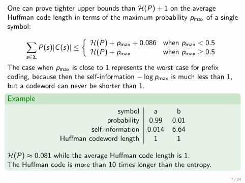
One can prove tighter upper bounds than H(P) + 1 on the averageHuffman code length in terms of the maximum probability pmax of a singlesymbol:

∑s∈Σ

P(s)|C (s)| ≤{H(P) + pmax + 0.086 when pmax < 0.5H(P) + pmax when pmax ≥ 0.5

The case when pmax is close to 1 represents the worst case for prefixcoding, because then the self-information − log pmax is much less than 1,but a codeword can never be shorter than 1.

Example

symbol a bprobability 0.99 0.01

self-information 0.014 6.64Huffman codeword length 1 1

H(P) ≈ 0.081 while the average Huffman code length is 1.The Huffman code is more than 10 times longer than the entropy.

7 / 24

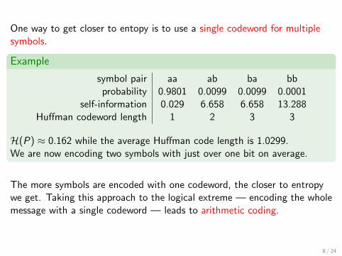
One way to get closer to entopy is to use a single codeword for multiplesymbols.

Example

symbol pair aa ab ba bbprobability 0.9801 0.0099 0.0099 0.0001

self-information 0.029 6.658 6.658 13.288Huffman codeword length 1 2 3 3

H(P) ≈ 0.162 while the average Huffman code length is 1.0299.We are now encoding two symbols with just over one bit on average.

The more symbols are encoded with one codeword, the closer to entropywe get. Taking this approach to the logical extreme — encoding the wholemessage with a single codeword — leads to arithmetic coding.

8 / 24

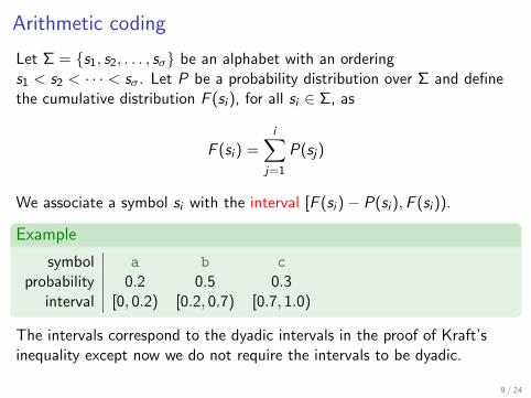
Arithmetic coding

Let Σ = {s1, s2, . . . , sσ} be an alphabet with an orderings1 < s2 < · · · < sσ. Let P be a probability distribution over Σ and definethe cumulative distribution F (si ), for all si ∈ Σ, as

F (si ) =i∑

j=1

P(sj)

We associate a symbol si with the interval [F (si )− P(si ),F (si )).

Example

symbol a b c

probability 0.2 0.5 0.3interval [0, 0.2) [0.2, 0.7) [0.7, 1.0)

The intervals correspond to the dyadic intervals in the proof of Kraft’sinequality except now we do not require the intervals to be dyadic.

9 / 24

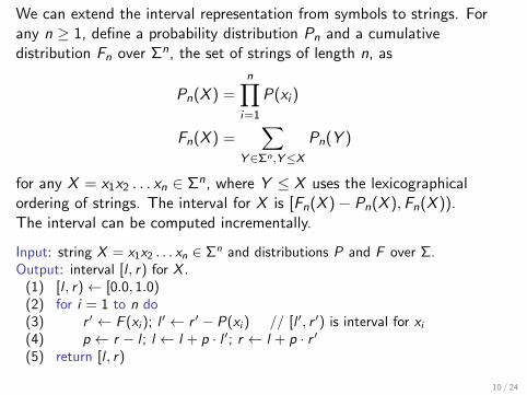
We can extend the interval representation from symbols to strings. Forany n ≥ 1, define a probability distribution Pn and a cumulativedistribution Fn over Σn, the set of strings of length n, as

Pn(X ) =n∏

i=1

P(xi )

Fn(X ) =∑

Y∈Σn,Y≤XPn(Y )

for any X = x1x2 . . . xn ∈ Σn, where Y ≤ X uses the lexicographicalordering of strings. The interval for X is [Fn(X )− Pn(X ),Fn(X )).The interval can be computed incrementally.

Input: string X = x1x2 . . . xn ∈ Σn and distributions P and F over Σ.Output: interval [l , r) for X .

(1) [l , r)← [0.0, 1.0)(2) for i = 1 to n do(3) r ′ ← F (xi ); l ′ ← r ′ − P(xi ) // [l ′, r ′) is interval for xi(4) p ← r − l ; l ← l + p · l ′; r ← l + p · r ′(5) return [l , r)

10 / 24

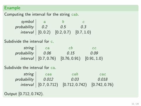
Example

Computing the interval for the string cab.

symbol a b c

probability 0.2 0.5 0.3interval [0, 0.2) [0.2, 0.7) [0.7, 1.0)

Subdivide the interval for c.

string ca cb cc

probability 0.06 0.15 0.09interval [0.7, 0.76) [0.76, 0.91) [0.91, 1.0)

Subdivide the interval for ca.

string caa cab cac

probability 0.012 0.03 0.018interval [0.7, 0.712) [0.712, 0.742) [0.742, 0.76)

Output [0.712, 0.742).

11 / 24

We can similarly associate an interval with each string over the codealphabet (which we assume to be binary here) but using equalprobabilities. The interval for a binary string B ∈ {0, 1}` is

I(B) =

[val(B)

2`,

val(B) + 1

2`

)where val(B) is the value of B as a binary number.

I This is the same interval as in the proof of Kraft’s inequality and isalways dyadic.

I Another characterization of I(B) is that it contains exactly allfractional binary numbers beginning with B. In fact, in the literature,arithmetic coding is often described using binary fractions instead ofintervals.

Example

For B = 101110, val(B) = 46 and thus

I(B) =

[46

64,

47

64

)= [.71875, .734375) = [.101110, .101111).

12 / 24

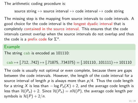
The arithmetic coding procedure is:

source string 7→ source interval 7→ code interval 7→ code string

The missing step is the mapping from source intervals to code intervals. Agood choice for the code interval is the longest dyadic interval that iscompletely contained in the source interval. This ensures that the codeintervals cannot overlap when the source intervals do not overlap and thusthe code is a prefix code for Σn.

Example

The string cab is encoded as 101110:

cab 7→ [.712, .742) 7→ [.71875, .734375) = [.101110, .101111) 7→ 101110

The code is usually not optimal or even complete, because there are gapsbetween the code intervals. However, the length of the code interval for asource interval of length p is always more than p/4. Thus the code lengthfor a string X is less than − log Pn(X ) + 2, and the average code length isless than H(Pn) + 2. Since H(Pn) = nH(P), the average code length persymbols is H(P) + 2/n.

13 / 24

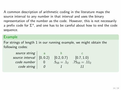
A common description of arithmetic coding in the literature maps thesource interval to any number in that interval and uses the binaryrepresentation of the number as the code. However, this is not necessarilya prefix code for Σn, and one has to be careful about how to end the codesequence.

Example

For strings of length 1 in our running example, we might obtain thefollowing codes:

source string a b c

source interval [0, 0.2) [0.2, 0.7) [0.7, 1.0)code number 0 .510 = .12 .7510 = .112

code string 0 1 11

14 / 24

A problematic issue with arithmetic coding is the potentially high precisionthat may be needed in the interval computations. The number of digitsrequired is proportional to the length of the final code string.

Practical implementations avoid high precision numbers using acombination of two techniques.

I Rouding: Replace high precision numbers with low precisionapproximations. As long as the final intervals for two distinct stringscan never overlap, the coding still works correctly. Rounding mayincrease the average code length, though.

I Renormalization: When the interval gets small enough, renormalize it,essentially “zooming in”. This way the intervals never get extremelysmall.

Practical implementations commonly use integer arithmetic both toimprove performance and to have full control of precision and the detailsof rounding.

15 / 24

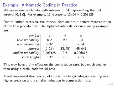
Example: Arithmetic Coding in PracticeWe use integer arithmetic with integers [0, 64] representing the unitinterval [0, 1.0]. For example, 13 represents 13/64 = 0.203125.

Due to limited precision, the interval sizes are not a perfect representationof the true probabilities. The alphabet intervals for our running exampleare:

symbol a b c

true probability 0.2 0.5 0.3self-information 2.32 1.0 1.74

interval [0, 13) [13, 45) [45, 64)implied probability 0.203125 0.5 0.296875

code length 2.30 1.0 1.75

This may have a tiny effect on the compression rate, but much smallerthan using a prefix code would have.

A real implementation would, of course, use larger integers resulting in ahigher precision and a smaller reduction in compression rate.

16 / 24

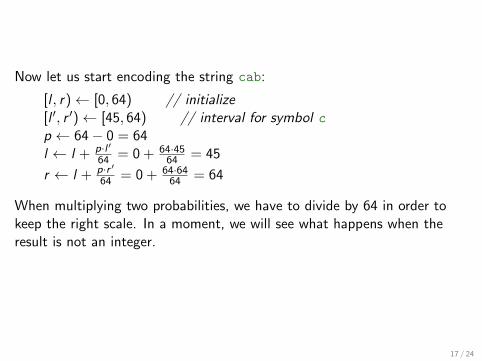
Now let us start encoding the string cab:

[l , r)← [0, 64) // initialize[l ′, r ′)← [45, 64) // interval for symbol cp ← 64− 0 = 64l ← l + p·l ′

64 = 0 + 64·4564 = 45

r ← l + p·r ′64 = 0 + 64·64

64 = 64

When multiplying two probabilities, we have to divide by 64 in order tokeep the right scale. In a moment, we will see what happens when theresult is not an integer.

17 / 24

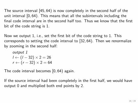
The source interval [45, 64) is now completely in the second half of theunit interval [0, 64). This means that all the subintervals including thefinal code interval are in the second half too. Thus we know that the firstbit of the code string is 1.

Now we output 1, i.e., set the first bit of the code string to 1. Thiscorresponds to setting the code interval to [32, 64). Then we renormalizeby zooming in the second half:

output 1l ← (l − 32)× 2 = 26r ← (r − 32)× 2 = 64

The code interval becomes [0, 64) again.

If the source interval had been completely in the first half, we would haveoutput 0 and multiplied both end points by 2.

18 / 24

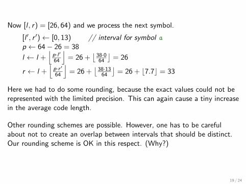
Now [l , r) = [26, 64) and we process the next symbol.

[l ′, r ′)← [0, 13) // interval for symbol ap ← 64− 26 = 38

l ← l +⌊p·l ′64

⌋= 26 +

⌊38·064

⌋= 26

r ← l +⌊p·r ′64

⌋= 26 +

⌊38·13

64

⌋= 26 + b7.7c = 33

Here we had to do some rounding, because the exact values could not berepresented with the limited precision. This can again cause a tiny increasein the average code length.

Other rounding schemes are possible. However, one has to be carefulabout not to create an overlap between intervals that should be distinct.Our rounding scheme is OK in this respect. (Why?)

19 / 24

Now [l , r) = [26, 33). This interval is not completely in the first half nor inthe second half. However, it is completely in the “middle” half [16, 48).Now we do not know what to output yet, but we still zoom in. Instead ofoutputting, we increment a variable called delayed bits (initialized to 0):

delayed bits← delayed bits + 1 = 1l ← (l − 16)× 2 = 20r ← (r − 16)× 2 = 34

[20, 34) is still in the middle half, so increment delayed bits andrenormalize again:

delayed bits← delayed bits + 1 = 2l ← (l − 16)× 2 = 8r ← (r − 16)× 2 = 36

Zooming in the middle half ensures that the length of the source intervalremains larger than one quarter of the unit interval, 16 in this case.

20 / 24

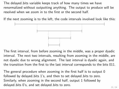
The delayed bits variable keeps track of how many times we haverenormalized without outputting anything. The output to produce will beresolved when we zoom in to the first or the second half.

If the next zooming is to the left, the code intervals involved look like this:

The first interval, from before zooming in the middle, was a proper dyadicinterval. The next two intervals, resulting from zooming in the middle, arenot dyadic due to wrong alignment. The last interval is dyadic again, andthe transition from the first to the last interval corresponds to the bits 011.

The general procedure when zooming in the first half is to output 0followed by delayed bits 1’s, and then to set delayed bits to zero.Similarly, when zooming in the second half, output 1 followed bydelayed bits 0’s, and set delayed bits to zero.

21 / 24

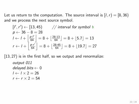
Let us return to the computation. The source interval is [l , r) = [8, 36)and we process the next source symbol.

[l ′, r ′)← [13, 45) // interval for symbol bp ← 36− 8 = 28

l ← l +⌊p·l ′64

⌋= 8 +

⌊28·13

64

⌋= 8 + b5.7c = 13

r ← l +⌊p·r ′64

⌋= 8 +

⌊28·45

64

⌋= 8 + b19.7c = 27

[13, 27) is in the first half, so we output and renormalize:

output 011delayed bits← 0l ← l × 2 = 26r ← r × 2 = 54

22 / 24

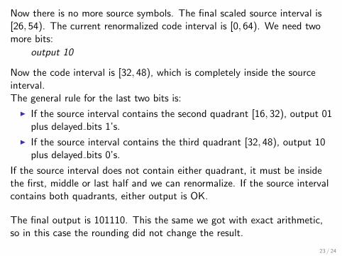
Now there is no more source symbols. The final scaled source interval is[26, 54). The current renormalized code interval is [0, 64). We need twomore bits:

output 10

Now the code interval is [32, 48), which is completely inside the sourceinterval.The general rule for the last two bits is:

I If the source interval contains the second quadrant [16, 32), output 01plus delayed bits 1’s.

I If the source interval contains the third quadrant [32, 48), output 10plus delayed bits 0’s.

If the source interval does not contain either quadrant, it must be insidethe first, middle or last half and we can renormalize. If the source intervalcontains both quadrants, either output is OK.

The final output is 101110. This the same we got with exact arithmetic,so in this case the rounding did not change the result.

23 / 24

Decoding arithmetic code performs much the same process, but theprocess is now controlled by the code string and it produces the sourcestring as output. Here is an outline of the decoding procedure in ourexample:

I We start with the code interval [0, 64). Each bit read from the codestring halves the code interval.

I In the beginning, the source interval is [0, 64) too, and it is dividedinto three candidate intervals: [0, 13), [13, 45) and [45, 64).

I Whenever the code interval falls within one of the candidate intervals,that interval becomes the new source interval and we output thecorresponding symbol.

I If the new source interval is within one of the three halves of the unitinterval, we renormalize scaling both the source and the code interval.

I The new source interval is divided into three candidate intervals andthe process continues.

I The process ends, when n symbols have been output.

The full details are left as an exercise.

24 / 24