2/2/01

Source Coding for Compression

Types of data compression:

1. Lossless -2. Lossy ­

(irreversible)

M1 Lec 16b.6-1

removes redundancies (reversible) removes less important information

2/2/01

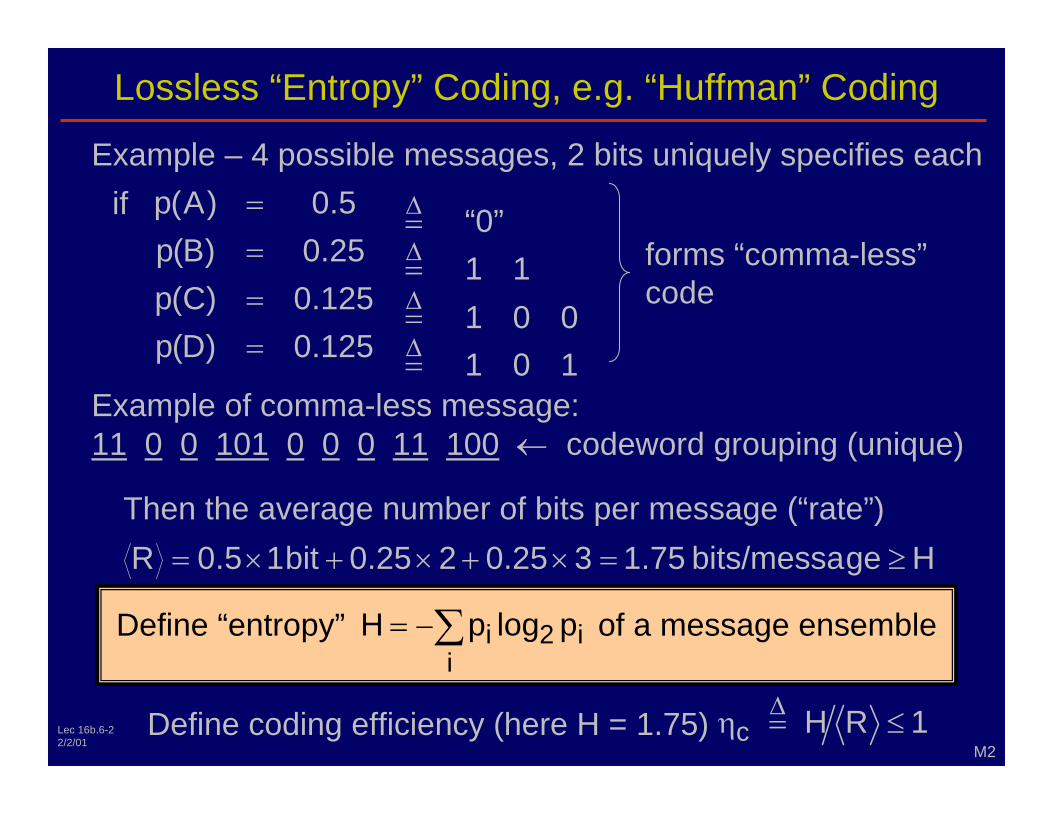
Lossless “Entropy” Coding, e.g. “Huffman” Coding

)D(p )C(p )B(p )A(p

=

=

=

=if ∆ = ∆ = ∆ = ∆ =

“0” 1 1 1 0 0 1 0 1

forms “comma-less” code

Example of comma-less message: 11 0 0 101 0 0 0 11 100 ← codeword grouping (unique)

Then the average number of bits per message (“rate”) H30.2520.25R ≥=×+×+×=

∑−= i

i2iHDefine “entropy”

c H R 1∆η = ≤Define coding efficiency (here H = 1.75) M2

Lec 16b.6-2

Example – 4 possible messages, 2 bits uniquely specifies each

125. 0 125. 0 25 . 0 5 . 0

ge bits/messa 1.75 bit 1 5. 0

p log p of a message ensemble

2/2/01

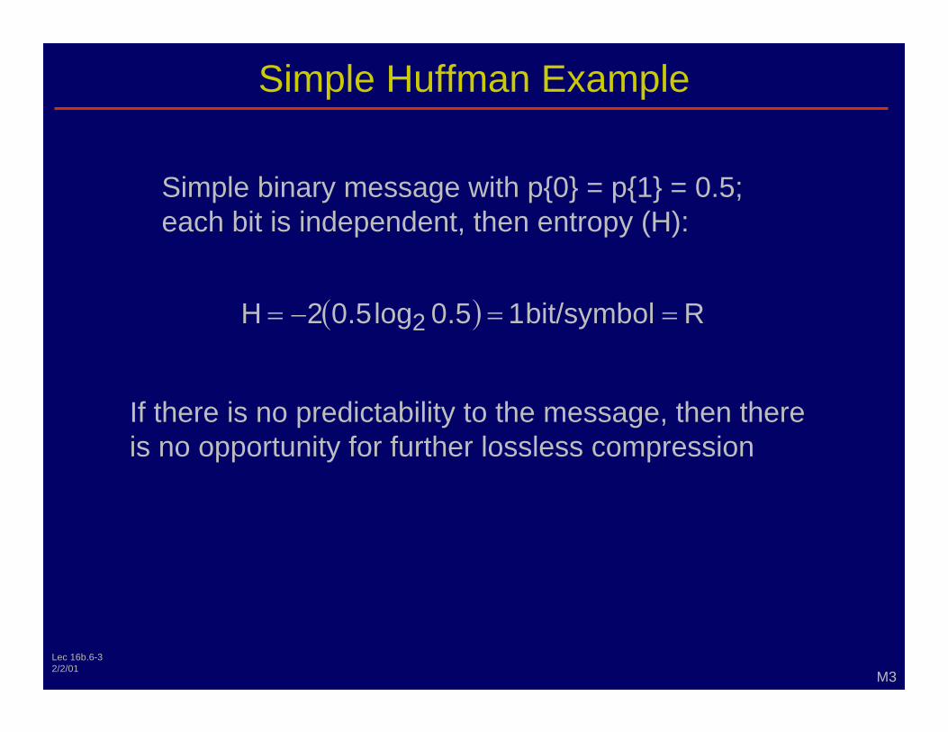
Simple Huffman Example

Simple binary message with p{0} = p{1} = 0.5; each bit is independent, then entropy (H):

( ) RH 2 ==

If there is no predictability to the message, then there is no opportunity for further lossless compression

M3 Lec 16b.6-3

bit/symbol 1 5 . 0 log 5 . 0 2 − =

2/2/01

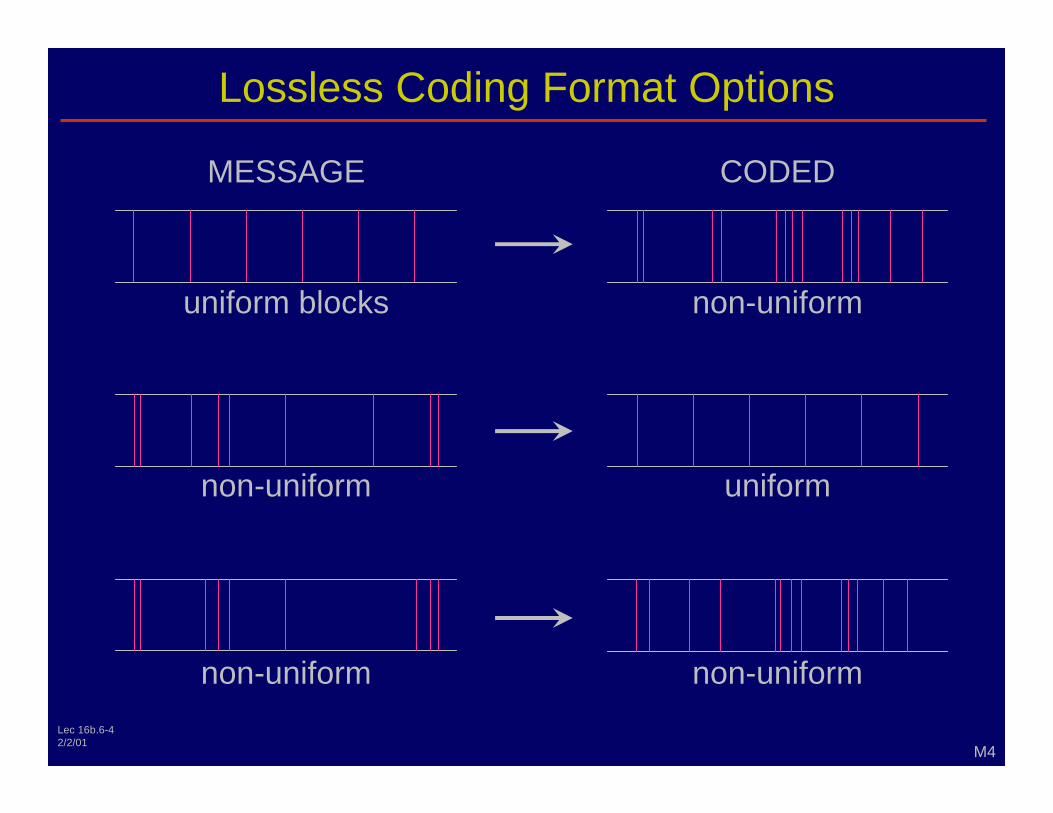
Lossless Coding Format Options

non-uniform

MESSAGE

uniform blocks

non-uniform

CODED

non-uniform

uniform

non-uniform

M4 Lec 16b.6-4

2/2/01

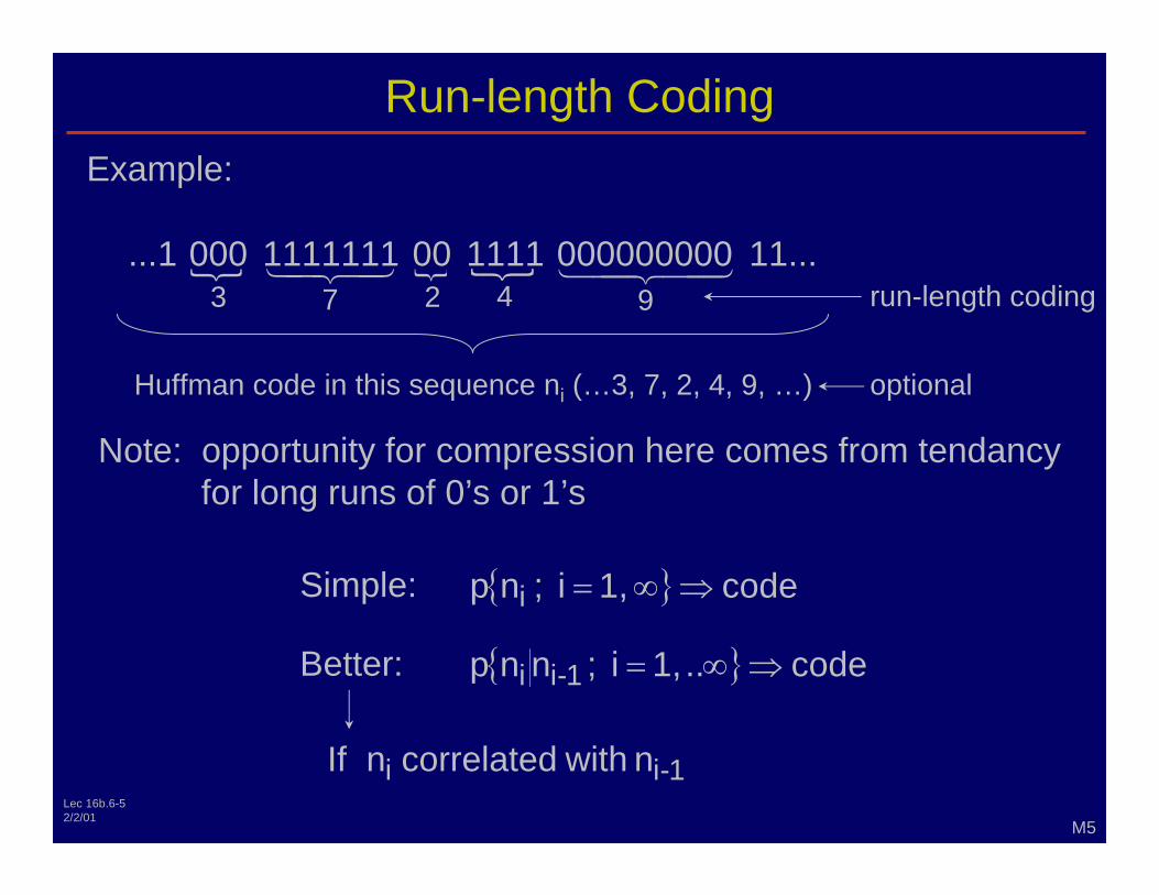
Run-length Coding Example:

N N N 94273 �����

Huffman code in this sequence ni (…3, 7, 2, 4, 9, …)

run-length coding

optional

Note: for long runs of 0’s or 1’s

{ } code1,i;i ⇒∞=

{ } codei;ii ⇒∞=

iiIf

Better:

Simple:

M5 Lec 16b.6-5

11... 000000000 1111 00 1111111 000 1 ... �� �

opportunity for compression here comes from tendancy

n p

.. 1, n n p 1­

1­n with correlated n

2/2/01

Other Popular Codes

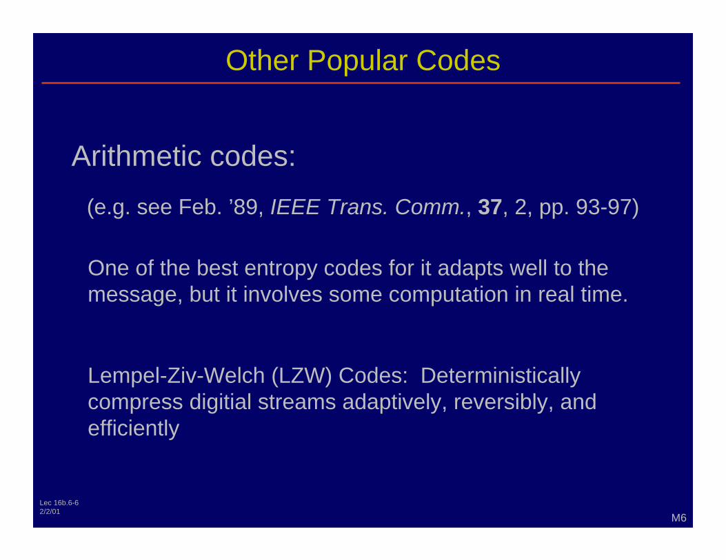
(e.g. see Feb. ’89, IEEE Trans. Comm., 37, 2, pp. 93-97)

Arithmetic codes:

One of the best entropy codes for it adapts well to the message, but it involves some computation in real time.

Lempel-Ziv-Welch (LZW) Codes: Deterministically

efficiently

M6 Lec 16b.6-6

compress digitial streams adaptively, reversibly, and

2/2/01

Information-Lossy Source Codes

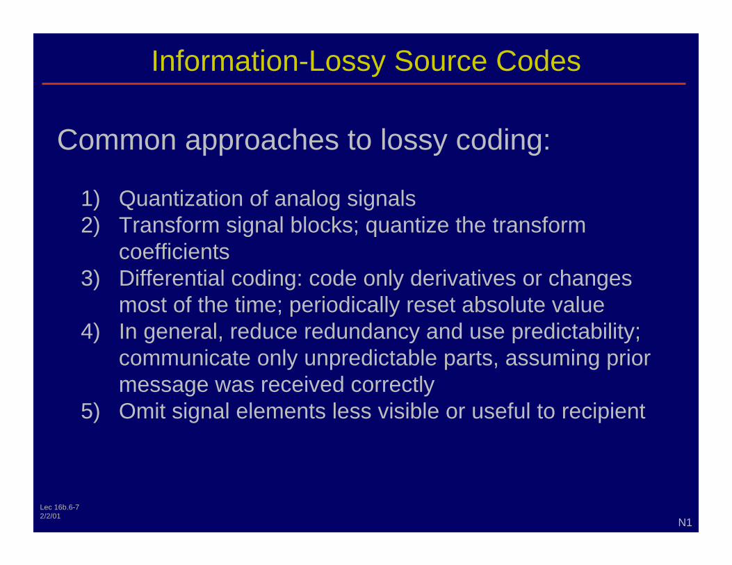
Common approaches to lossy coding:

coefficients

most of the time; periodically reset absolute value

message was received correctly

N1 Lec 16b.6-7

1) Quantization of analog signals 2) Transform signal blocks; quantize the transform

3) Differential coding: code only derivatives or changes

4) In general, reduce redundancy and use predictability; communicate only unpredictable parts, assuming prior

5) Omit signal elements less visible or useful to recipient

2/2/01

Discrete Fourier Transform (DFT):

( )∑ −

=

π−= 0k

e)k(x)n(X

] e.g

( )∑ −

=

π= 0n

e)n(XN 1)k(x Inverse DFT “IDFT”

n = 2

N2

n = 0

Note: X(n) is complex ↔ 2N #’s

0 sharp edges of window ⇒

reconstructed decoded signal

n = 1

Lec 16b.6-8

Transform Codes - DFT

1 N N k 2 jn

[n = 0, 1, …, N – 1

1 N N k 2 jn

“ringing” or “sidelobes in the

2/2/01

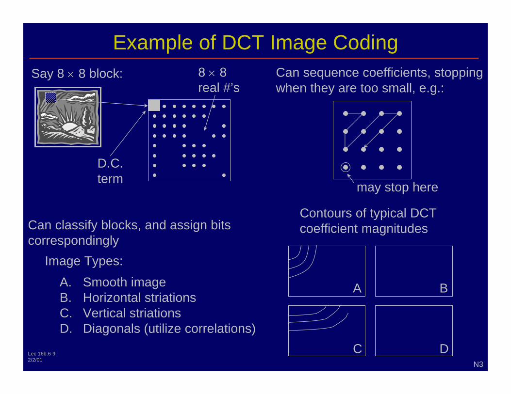
Example of DCT Image Coding Say 8 ×

term

8 × 8 real #’s

may stop here

Can sequence coefficients, stopping when they are too small, e.g.:

correspondingly Image Types:

A. Smooth image B. Horizontal striations C. Vertical striations D.

coefficient magnitudes

A B

C D N3

Lec 16b.6-9

8 block:

D.C.

Can classify blocks, and assign bits

Diagonals (utilize correlations)

Contours of typical DCT

2/2/01

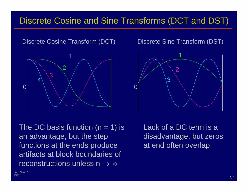
Discrete Cosine and Sine Transforms (DCT and DST)

0 4

3 2

1

The DC basis function (n = 1) is an advantage, but the step functions at the ends produce artifacts at block boundaries of reconstructions unless n → ∞

N4

Lack of a DC term is a disadvantage, but zeros at end often overlap

0 3

2

1

Lec 16b.6-10

Discrete Cosine Transform (DCT) Discrete Sine Transform (DST)

2/2/01

Lapped Transforms

N5

block

extended block

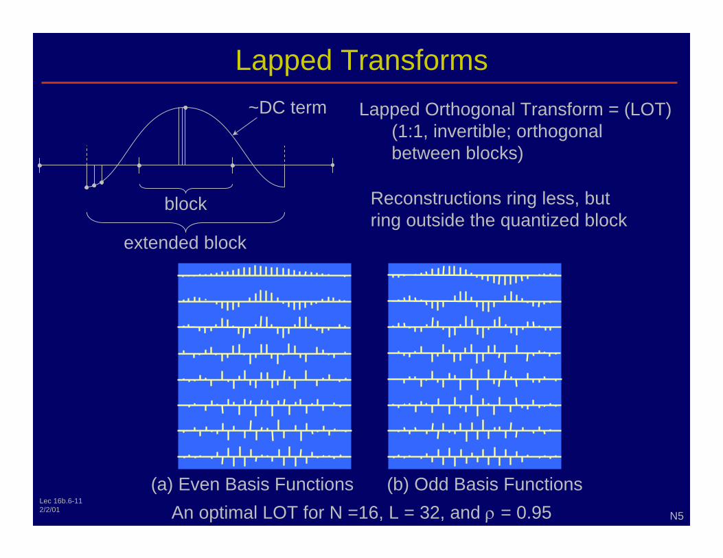
~DC term Lapped Orthogonal Transform = (LOT) (1:1, invertible; orthogonal between blocks)

Reconstructions ring less, but ring outside the quantized block

(a) Even Basis Functions (An optimal LOT for N =16, L = 32, and ρ = 0.95

Lec 16b.6-11

b) Odd Basis Functions

2/2/01

Lapped Transforms

N6

t

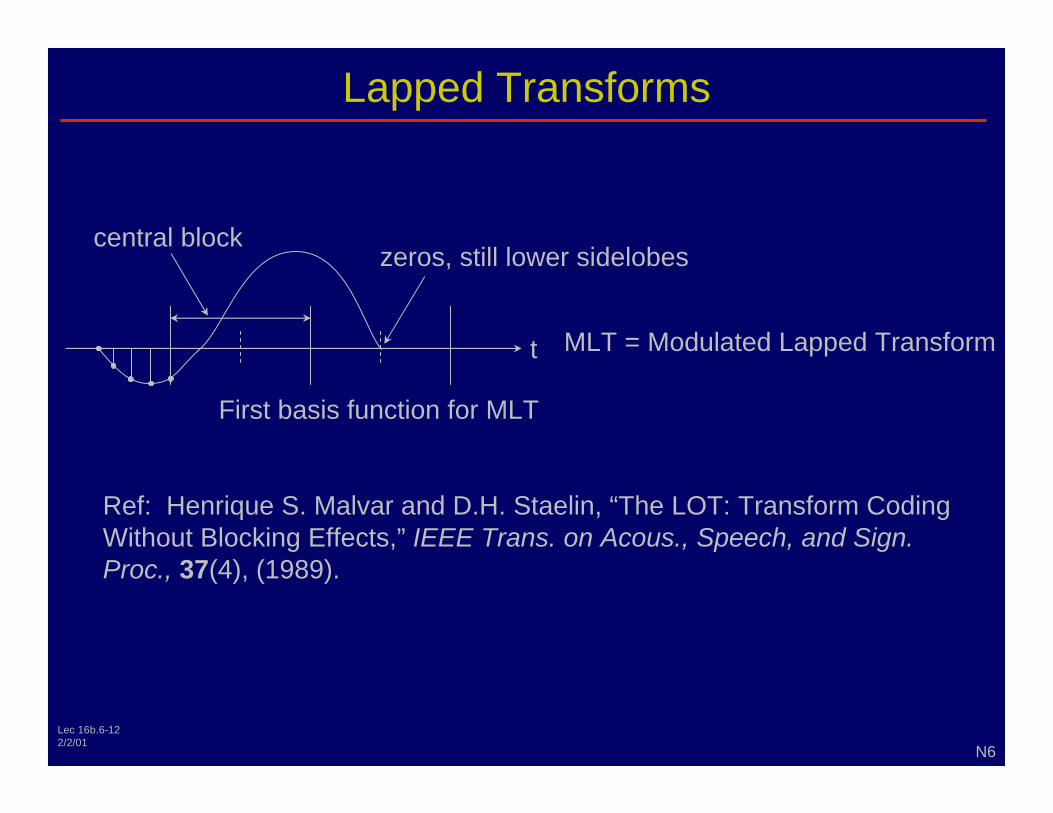
central block zeros, still lower sidelobes

First basis function for MLT

MLT = Modulated Lapped Transform

Ref: IEEE Trans. on Acous., Speech, and Sign.

Proc., 37(4), (1989).

Lec 16b.6-12

Henrique S. Malvar and D.H. Staelin, “The LOT: Transform Coding Without Blocking Effects,”

2/2/01

Karhounen-Loéve Transform (KLT)

Example:

0 n

0 j

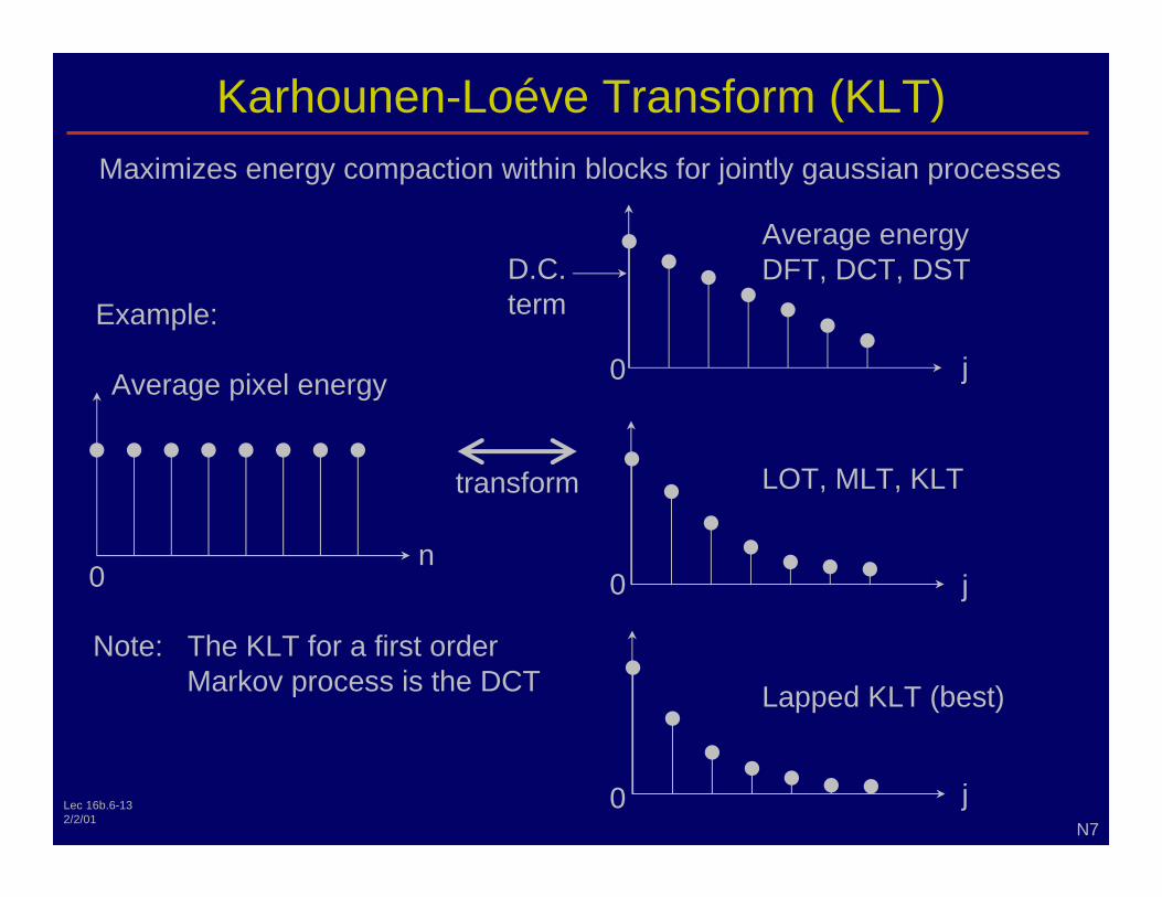
Average energy DFT, DCT, DST

term

transform

N7

Note: The KLT for a first order Markov process is the DCT

0 j

LOT, MLT, KLT

0 j

Lapped KLT (best)

Lec 16b.6-13

Maximizes energy compaction within blocks for jointly gaussian processes

Average pixel energy

D.C.

2/2/01

Vector Quntization (“VQ”)

P1

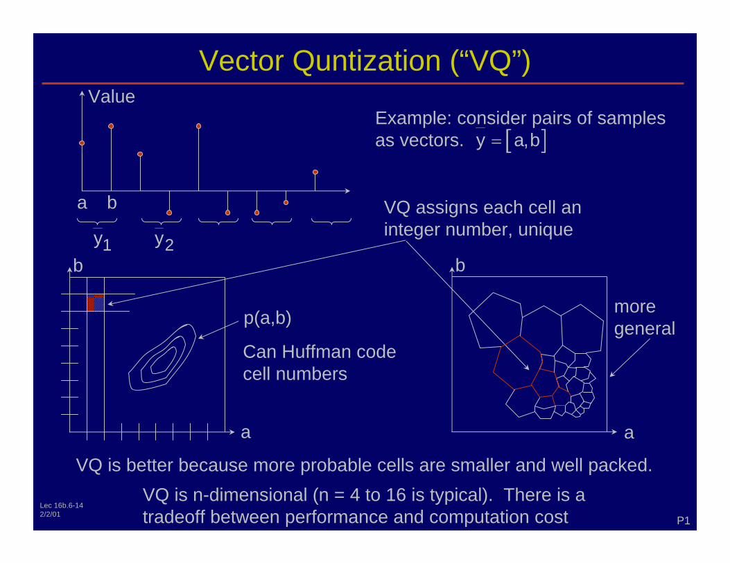
Example: consider pairs of samples as vectors. [ ]y =

1y 2y

a b

Value

VQ assigns each cell an integer number, unique

There is a tradeoff between performance and computation cost

p(a,b)

Can Huffman code cell numbers

a

b

VQ is better because more probable cells are smaller and well packed.

b

a

more general

Lec 16b.6-14

a,b

VQ is n-dimensional (n = 4 to 16 is typical).

2/2/01

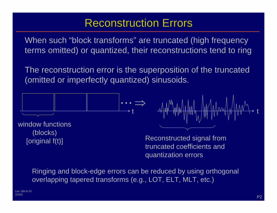
Reconstruction Errors When such “block transforms” are truncated (high frequency terms omitted) or quantized, their reconstructions tend to ring

The reconstruction error is the superposition of the truncated (omitted or imperfectly quantized) sinusoids.

t ⇒

t

Reconstructed signal from truncated coefficients and quantization errors

window functions (blocks)

[original f(t)]

P2 Lec 16b.6-15

Ringing and block-edge errors can be reduced by using orthogonal overlapping tapered transforms (e.g., LOT, ELT, MLT, etc.)

2/2/01

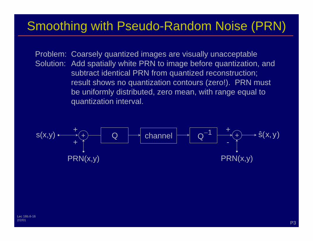
Smoothing with Pseudo-Random Noise (PRN)

P3

Problem:

subtract identical PRN from quantized reconstruction; PRN must

be uniformly distributed, zero mean, with range equal to quantization interval.

s(x,y)

PRN(x,y)

ˆ )1Q−+ Q channel +

PRN(x,y)

+ +

-+

Lec 16b.6-16

Coarsely quantized images are visually unacceptable Solution: Add spatially white PRN to image before quantization, and

result shows no quantization contours (zero!).

s(x, y

2/2/01

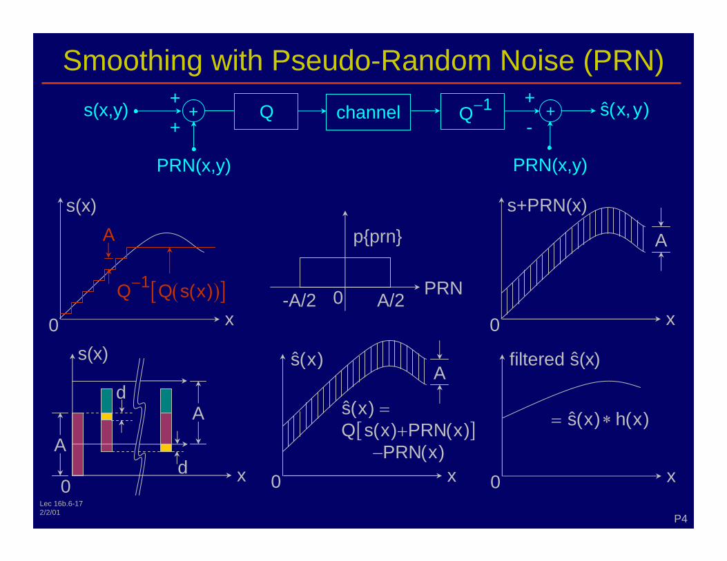
Smoothing with Pseudo-Random Noise (PRN) s(x,y)

PRN(x,y)

ˆ )1Q−+ Q channel +

PRN(x,y)

PRN-A/2 A/20

p{prn}

s+PRN(x)

x0

A

s(x)

x0

( )[ ]1Q (x)−

x0

ˆfil (x)

s(x) h(x)= ∗

x0

s(x)

A

A d

d x0

ˆ )

[ ] ˆ )

) ) (x)

= +

−

A

P4

+ +

-+

A

Lec 16b.6-17

s(x, y

Q s

tered ss(x

s(xQ s(x PRN(x

PRN

2/2/01

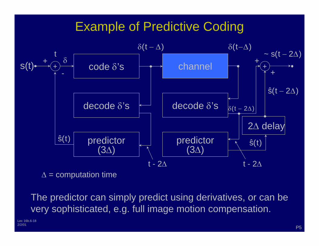
Example of Predictive Coding

+

2∆ delay

code δ’s

decode δ’s

predictor(3∆)

channel

decode δ’s

predictor(3∆)

+s(t)

ˆ )

(t )δ − ∆ (t )δ −∆ t

+ δ

-

∆ ∆

ˆ )

+ +

− ∆ˆ 2 )

− ∆~ s(t 2 )

∆ = computation time

The predictor can simply predict using derivatives, or can be very sophisticated, e.g. full image motion compensation.

P5

δ − ∆(t 2 )

Lec 16b.6-18

s(t

t - 2 t - 2

s(t

s(t

2/2/01

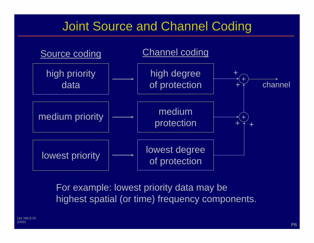
Joint Source and Channel Coding

For example: lowest priority data may be highest spatial (or time) frequency components.

Source coding Channel coding

high priority data

medium priority

lowest priority

high degree of protection

medium protection

lowest degree of protection

+

+

+ +

+ +

channel

P6 Lec 16b.6-19

2/2/01

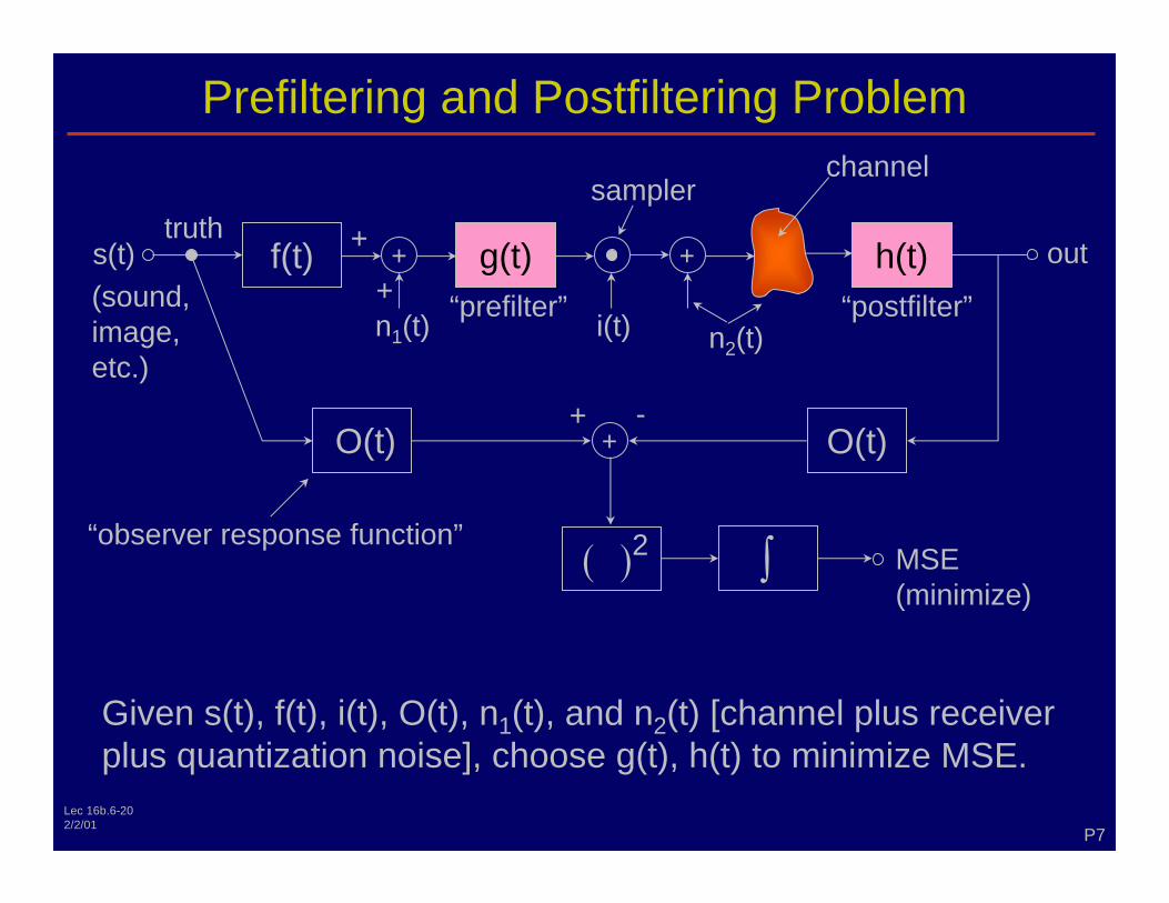
Prefiltering and Postfiltering Problem

P7

f(t) g(t) h(t)+ + truth

sampler channel

outs(t) (sound, image, etc.)

“prefilter” i(t) n2(t)n1(t)

+

+

Given s(t), f(t), i(t), O(t), n1(t), and n2(t) [channel plus receiver plus quantization noise], choose g(t), h(t) to minimize MSE.

O(t)O(t) +

“observer response function” MSE (minimize)

( )2 ∫

+ -

Lec 16b.6-20

“postfilter”

2/2/01

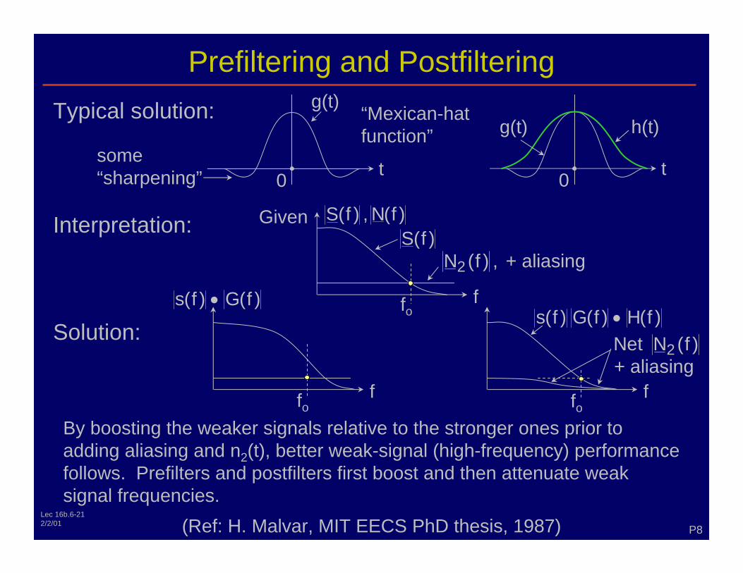
Prefiltering and Postfiltering Typical solution:

t0 some “sharpening”

g(t) “Mexican-hat function”

t0

g(t) h(t)

P8

adding aliasing and n2

signal frequencies. (Ref: H. Malvar, MIT EECS PhD thesis, 1987)

Interpretation:

Solution: f

ffo ffo

Given

fo

) , N(f )

) G(f )• s(f ) G(f ) H(f )•

) 2N (f )

2N (f ) + ali i

Lec 16b.6-21

By boosting the weaker signals relative to the stronger ones prior to (t), better weak-signal (high-frequency) performance

follows. Prefilters and postfilters first boost and then attenuate weak

S(f

s(f

S(f , + aliasing

Netas ng

2/2/01

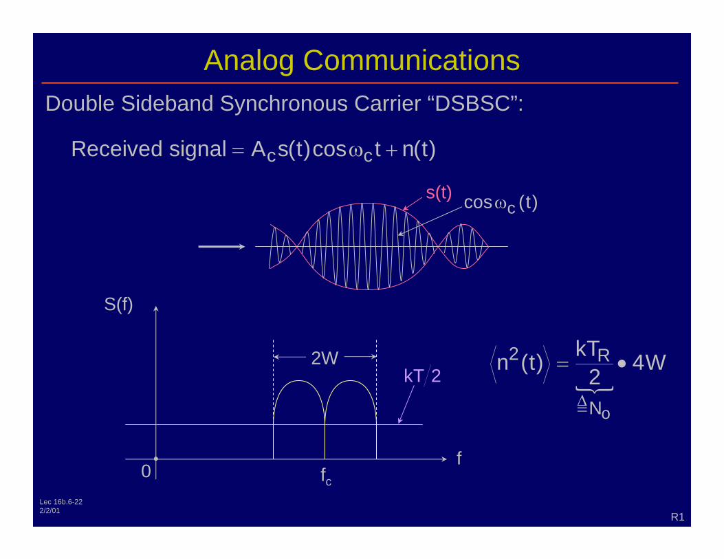
Analog Communications Double Sideband Synchronous Carrier “DSBSC”:

c ci ignal (t) t n(t)= ω +

N o

2 R

N

kT) 2 ∆=

= •

R1

s(t) c (t)ω

2W

0 fc

f

S(f)

Lec 16b.6-22

Rece ved s A s cos

n (t 4W

cos

kT 2

2/2/01

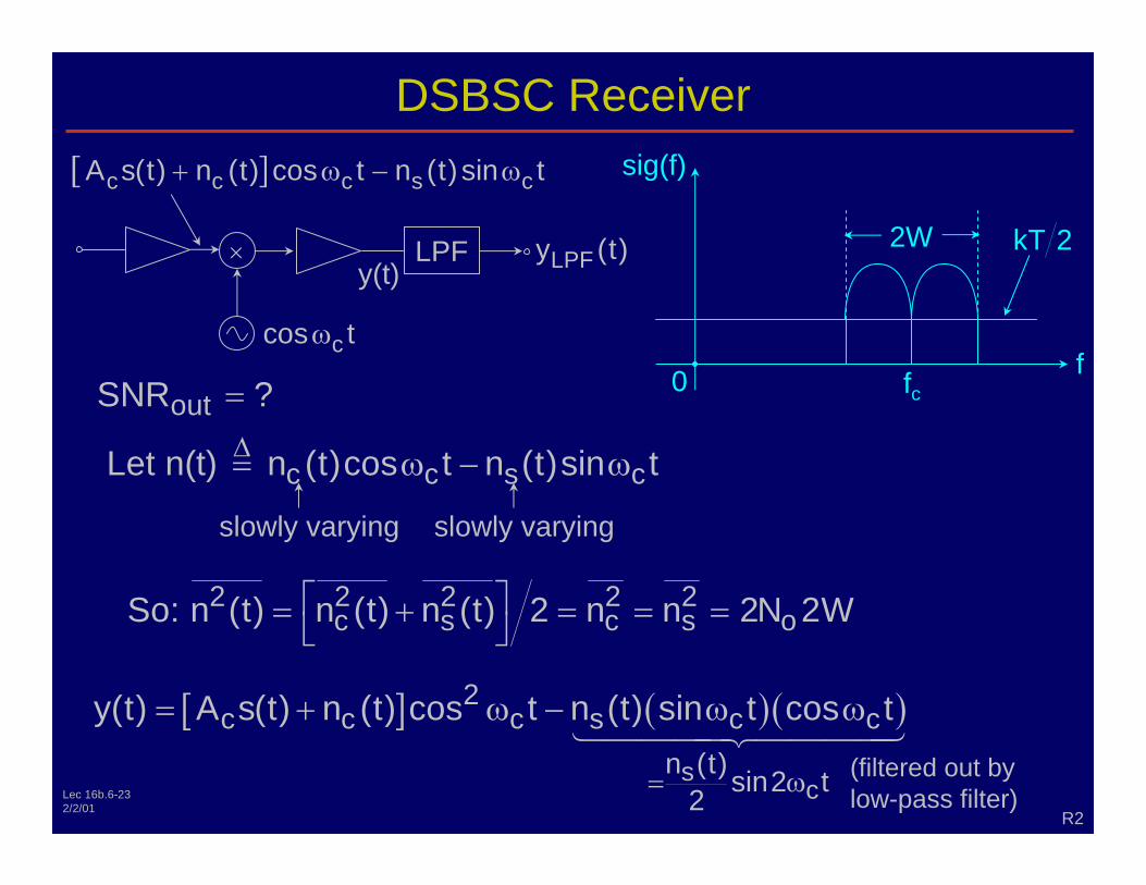
DSBSC Receiver

× LPF 2W

0 fc f

sig(f)[ ]c c c s cA ) n (t) t ) sin t+ ω

LPFy (t)

c tω

y(t)

c c s cn (t) t n (t)sin t∆ = ω

2 2 2 2 2 c s c s o) ) ) 2 n n⎡ ⎤= + = = =

⎣ ⎦

out ?=

slowly varying slowly varying

[ ] ( )( ) s

c

2 c c c s c c

) t2

y(t) ) ) t ) sin t t

= ω

= + ω ω ���� (filtered out by low-pass filter)

R2 Lec 16b.6-23

kT 2

s(t cos n (tω −

cos

Let n(t) cos ω −

So: n (t n (t n (t 2N 2W

SNR

n (t sin 2

A s(t n (t cos n (t cos ω − �����

2/2/01

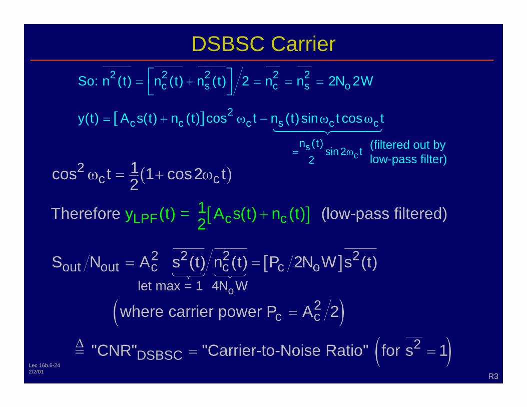
DSBSC Carrier 2 2 2 2 2

c s c s o(t) n (t) n (t) 2 n n= + = = =⎡ ⎤⎣ ⎦

[ ]

s c

2 c c c s c c

) t

2

y(t) A n t in t

= ω

= + ω ω �(filtered out by low-pass filter)

( )2 c c

1t 1 t2ω = + ω

[ ]LPF c c 1y (t) = (t) (l ltn ( et) )2 +

[ ]2 2 2 2 out out c c c oS N A s ( (t) P (t)= =

let max = 1 o

( )2 c ci A 2=

( )2i 1∆ = = =

R3 Lec 16b.6-24

So: n 2N 2W

n (tsin 2

s(t) (t) cos n (t) s t cos ω − ����

cos cos 2

A sTherefore ow-pass fi red

t) n 2N W s 4N W

where carr er power P

DSBSC "CNR" "Carrier-to-Noise Rat o" for s

2/2/01

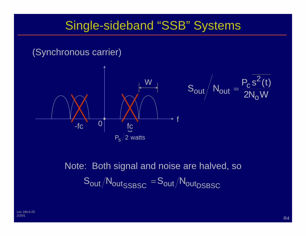
Single-sideband “SSB” Systems

2 c

out o

P s (t)S N =

Note: Both signal and noise are halved, so

SSBSCout outS N S N=

(Synchronous carrier)

0-fc N sP

fc f

W

R4 Lec 16b.6-25

out 2N W

DSBSC out out

2 watts