CS 229, Public Course Problem Set #2 Solutions: Kernels...

CS229 Problem Set #2 Solutions 1

CS 229, Public Course

Problem Set #2 Solutions: Kernels, SVMs, andTheory

1. Kernel ridge regression

In contrast to ordinary least squares which has a cost function

J(θ) =1

2

m∑

i=1

(θT x(i) − y(i))2,

we can also add a term that penalizes large weights in θ. In ridge regression, our leastsquares cost is regularized by adding a term λ‖θ‖2, where λ > 0 is a fixed (known) constant(regularization will be discussed at greater length in an upcoming course lecutre). The ridgeregression cost function is then

J(θ) =1

2

m∑

i=1

(θT x(i) − y(i))2 +λ

2‖θ‖2.

(a) Use the vector notation described in class to find a closed-form expreesion for thevalue of θ which minimizes the ridge regression cost function.

Answer: Using the design matrix notation, we can rewrite J(θ) as

J(θ) =1

2(Xθ − ~y)T (Xθ − ~y) +

λ

2θT θ.

Then the gradient is∇θJ(θ) = XT Xθ − XT ~y + λθ.

Setting the gradient to 0 gives us

0 = XT Xθ − XT ~y + λθ

θ = (XT X + λI)−1XT ~y.

(b) Suppose that we want to use kernels to implicitly represent our feature vectors in ahigh-dimensional (possibly infinite dimensional) space. Using a feature mapping φ,the ridge regression cost function becomes

J(θ) =1

2

m∑

i=1

(θT φ(x(i)) − y(i))2 +λ

2‖θ‖2.

Making a prediction on a new input xnew would now be done by computing θT φ(xnew).Show how we can use the “kernel trick” to obtain a closed form for the predictionon the new input without ever explicitly computing φ(xnew). You may assume thatthe parameter vector θ can be expressed as a linear combination of the input featurevectors; i.e., θ =

∑mi=1 αiφ(x(i)) for some set of parameters αi.


[Hint: You may find the following identity useful:

(λI + BA)−1B = B(λI + AB)−1.

If you want, you can try to prove this as well, though this is not required for theproblem.]

Answer: Let Φ be the design matrix associated with the feature vectors φ(x(i)). Thenfrom parts (a) and (b),

θ =(

ΦT Φ + λI)−1

ΦT ~y

= ΦT(

ΦΦT + λI)−1

~y

= ΦT (K + λI)−1~y.

where K is the kernel matrix for the training set (since Φi,j = φ(x(i))T φ(x(j)) = Kij .)To predict a new value ynew, we can compute

~ynew = θT φ(xnew)

= ~yT (K + λI)−1Φφ(xnew)

=

m∑

i=1

αiK(x(i), xnew).

where α = (K + λI)−1~y. All these terms can be efficiently computing using the kernelfunction.

To prove the identity from the hint, we left-multiply by λ(I + BA) and right-multiply byλ(I + AB) on both sides. That is,

(λI + BA)−1B = B(λI + AB)−1

B = (λI + BA)B(λI + AB)−1

B(λI + AB) = (λI + BA)B

λB + BAB = λB + BAB.

This last line clearly holds, proving the identity.

2. ℓ2 norm soft margin SVMs

In class, we saw that if our data is not linearly separable, then we need to modify oursupport vector machine algorithm by introducing an error margin that must be minimized.Specifically, the formulation we have looked at is known as the ℓ1 norm soft margin SVM.In this problem we will consider an alternative method, known as the ℓ2 norm soft marginSVM. This new algorithm is given by the following optimization problem (notice that theslack penalties are now squared):

minw,b,ξ12‖w‖2 + C

2

∑mi=1 ξ2

i

s.t. y(i)(wT x(i) + b) ≥ 1 − ξi, i = 1, . . . ,m.

(a) Notice that we have dropped the ξi ≥ 0 constraint in the ℓ2 problem. Show that thesenon-negativity constraints can be removed. That is, show that the optimal value ofthe objective will be the same whether or not these constraints are present.

Answer: Consider a potential solution to the above problem with some ξ < 0. Thenthe constraint y(i)(wT x(i) + b) ≥ 1 − ξi would also be satisfied for ξi = 0, and theobjective function would be lower, proving that this could not be an optimal solution.


(b) What is the Lagrangian of the ℓ2 soft margin SVM optimization problem?

Answer:

L(w, b, ξ, α) =1

2wT w +

C

2

m∑

i=1

ξ2i −

m∑

i=1

αi[y(i)(wT x(i) + b) − 1 + ξi],

where αi ≥ 0 for i = 1, . . . ,m.

(c) Minimize the Lagrangian with respect to w, b, and ξ by taking the following gradients:∇wL, ∂L

∂b, and ∇ξL, and then setting them equal to 0. Here, ξ = [ξ1, ξ2, . . . , ξm]T .

Answer: Taking the gradient with respect to w, we get

0 = ∇wL = w −

m∑

i=1

αiy(i)x(i),

which gives us

w =

m∑

i=1

αiy(i)x(i).

Taking the derivative with respect to b, we get

0 =∂L

∂b= −

m∑

i=1

αiy(i),

giving us

0 =m∑

i=1

αiy(i).

Finally, taking the gradient with respect to ξ, we have

0 = ∇ξL = Cξ − α,

where α = [α1, α2, . . . , αm]T . Thus, for each i = 1, . . . ,m, we get

0 = Cξi − αi ⇒ Cξi = αi.

(d) What is the dual of the ℓ2 soft margin SVM optimization problem?


Answer: The objective function for the dual is

W (α) = minw,b,ξ

L(w, b, ξ, α)

=1

2

m∑

i=1

m∑

j=1

(αiy(i)x(i))T (αjy

(j)x(j)) +1

2

m∑

i=1

αi

ξi

ξ2i

−

m∑

i=1

αi

y(i)

m∑

j=1

αjy(j)x(j)

T

x(i) + b

− 1 + ξi

= −1

2

m∑

i=1

m∑

j=1

αiαjy(i)y(j)(x(i))T x(j) +

1

2

m∑

i=1

αiξi

−

(

m∑

i=1

αiy(i)

)

b +

m∑

i=1

αi −

m∑

i=1

αiξi

=

m∑

i=1

αi −1

2

m∑

i=1

m∑

j=1

αiαjy(i)y(j)(x(i))T x(j) −

1

2

m∑

i=1

αiξi

=m∑

i=1

αi −1

2

m∑

i=1

m∑

j=1

αiαjy(i)y(j)(x(i))T x(j) −

1

2

m∑

i=1

α2i

C.

Then the dual formulation of our problem is

maxα

∑mi=1 αi −

12

∑mi=1

∑mj=1 αiαjy

(i)y(j)(x(i))T x(j) − 12

∑mi=1

α2

i

C

s.t. αi ≥ 0, i = 1, . . . ,m∑m

i=1 αiy(i) = 0

.

3. SVM with Gaussian kernel

Consider the task of training a support vector machine using the Gaussian kernel K(x, z) =exp(−‖x − z‖2/τ2). We will show that as long as there are no two identical points in thetraining set, we can always find a value for the bandwidth parameter τ such that the SVMachieves zero training error.

(a) Recall from class that the decision function learned by the support vector machinecan be written as

f(x) =m∑

i=1

αiy(i)K(x(i), x) + b.

Assume that the training data {(x(1), y(1)), . . . , (x(m), y(m))} consists of points whichare separated by at least a distance of ǫ; that is, ||x(j) − x(i)|| ≥ ǫ for any i 6= j.Find values for the set of parameters {α1, . . . , αm, b} and Gaussian kernel width τsuch that x(i) is correctly classified, for all i = 1, . . . ,m. [Hint: Let αi = 1 for all iand b = 0. Now notice that for y ∈ {−1,+1} the prediction on x(i) will be correct if|f(x(i)) − y(i)| < 1, so find a value of τ that satisfies this inequality for all i.]


Answer: First we set αi = 1 for all i = 1, . . . ,m and b = 0. Then, for a trainingexample {x(i), y(i)}, we get

∣

∣

∣f(x(i)) − y(i)∣

∣

∣ =

∣

∣

∣

∣

∣

∣

m∑

j=1

y(j)K(x(j), x(i)) − y(i)

∣

∣

∣

∣

∣

∣

=

∣

∣

∣

∣

∣

∣

m∑

j=1

y(j) exp(

−‖x(j) − x(i)‖2/τ2)

− y(i)

∣

∣

∣

∣

∣

∣

=

∣

∣

∣

∣

∣

∣

y(i) +∑

j 6=i

y(j) exp(

‖x(j) − x(i)‖2/τ2)

− y(i)

∣

∣

∣

∣

∣

∣

=

∣

∣

∣

∣

∣

∣

∑

j 6=i

y(j) exp(

−‖x(j) − x(i)‖2/τ2)

∣

∣

∣

∣

∣

∣

≤∑

j 6=i

∣

∣

∣y(j) exp

(

−‖x(j) − x(i)‖2/τ2)∣

∣

∣

=∑

j 6=i

∣

∣

∣y(j)∣

∣

∣ · exp(

‖x(j) − x(i)‖2/τ2)

=∑

j 6=i

exp(

−‖x(j) − x(i)‖2/τ2)

≤∑

j 6=i

exp(

−ǫ2/τ2)

= (m − 1) exp(

−ǫ2/τ2)

.

The first inequality comes from repeated application of the triangle inequality |a + b| ≤|a|+ |b|, and the second inequality (1) from the assumption that ||x(j) − x(i)|| ≥ ǫ for alli 6= j. Thus we need to choose a γ such that

(m − 1) exp(−ǫ2/τ2) < 1,

orτ <

ǫ

log(m − 1).

By choosing, for example, τ = ǫ/ log m we are done.

(b) Suppose we run a SVM with slack variables using the parameter τ you found in part(a). Will the resulting classifier necessarily obtain zero training error? Why or whynot? A short explanation (without proof) will suffice.

Answer: The classifier will obtain zero training error. The SVM without slack variableswill always return zero training error if it is able to find a solution, so all that remains tobe shown is that there exists at least one feasible point.

Consider the constraint y(i)(wT x(i) + b) for some i, and let b = 0. Then

y(i)(wT x(i) + b) = y(i) · f(x(i)) > 0

since f(x(i)) and y(i) have the same sign, and shown above. Therefore, as we choose allthe αi’s large enough, y(i)(wT x(i) + b) > 1, so the optimization problem is feasible.


(c) Suppose we run the SMO algorithm to train an SVM with slack variables, underthe conditions stated above, using the value of τ you picked in the previous part,and using some arbitrary value of C (which you do not know beforehand). Will thisnecessarily result in a classifier that achieve zero training error? Why or why not?Again, a short explanation is sufficient.

Answer: The resulting classifier will not necessarily obtain zero training error. The Cparameter controls the relative weights of the (C

∑mi=1 ξi) and (1

2 ||w||2) terms of the SVMtraining objective. If the C parameter is sufficiently small, then the former component willhave relatively little contribution to the objective. In this case, a weight vector which hasa very small norm but does not achieve zero training error may achieve a lower objectivevalue than one which achieves zero training error. For example, you can consider theextreme case where C = 0, and the objective is just the norm of w. In this case, w = 0 isthe solution to the optimization problem regardless of the choise of τ , this this may notobtain zero training error.

4. Naive Bayes and SVMs for Spam Classification

In this question you’ll look into the Naive Bayes and Support Vector Machine algorithmsfor a spam classification problem. However, instead of implementing the algorithms your-self, you’ll use a freely available machine learning library. There are many such librariesavailable, with different strengths and weaknesses, but for this problem you’ll use theWEKA machine learning package, available at http://www.cs.waikato.ac.nz/ml/weka/.WEKA implements many standard machine learning algorithms, is written in Java, andhas both a GUI and a command line interface. It is not the best library for very large-scaledata sets, but it is very nice for playing around with many different algorithms on mediumsize problems.

You can download and install WEKA by following the instructions given on the websiteabove. To use it from the command line, you first need to install a java runtime environ-ment, then add the weka.jar file to your CLASSPATH environment variable. Finally, youcan call WEKA using the command:java <classifier> -t <training file> -T <test file>

For example, to run the Naive Bayes classifier (using the multinomial event model) on ourprovided spam data set by running the command:java weka.classifiers.bayes.NaiveBayesMultinomial -t spam train 1000.arff -T spam test.arff

The spam classification dataset in the q4/ directory was provided courtesy of ChristianShelton ([email protected]). Each example corresponds to a particular email, and eachfeature correspondes to a particular word. For privacy reasons we have removed the actualwords themselves from the data set, and instead label the features generically as f1, f2, etc.However, the data set is from a real spam classification task, so the results demonstrate theperformance of these algorithms on a real-world problem. The q4/ directory actually con-tains several different training files, named spam train 50.arff, spam train 100.arff,etc (the “.arff” format is the default format by WEKA), each containing the correspondingnumber of training examples. There is also a single test set spam test.arff, which is ahold out set used for evaluating the classifier’s performance.

(a) Run the weka.classifiers.bayes.NaiveBayesMultinomial classifier on the datasetand report the resulting error rates. Evaluate the performance of the classifier usingeach of the different training files (but each time using the same test file, spam test.arff).Plot the error rate of the classifier versus the number of training examples.


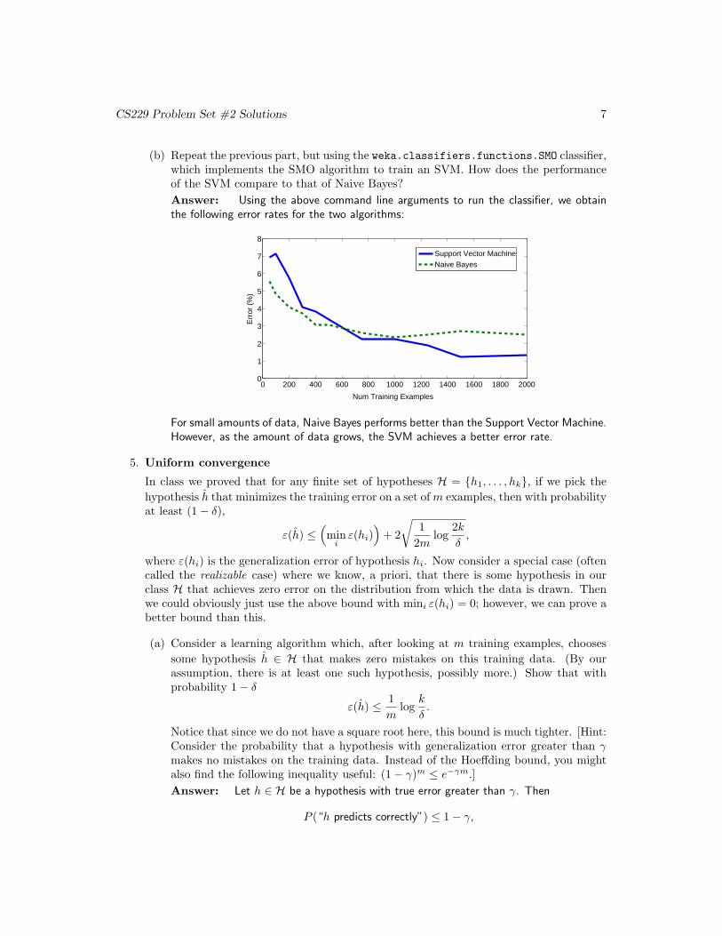
(b) Repeat the previous part, but using the weka.classifiers.functions.SMO classifier,which implements the SMO algorithm to train an SVM. How does the performanceof the SVM compare to that of Naive Bayes?

Answer: Using the above command line arguments to run the classifier, we obtainthe following error rates for the two algorithms:

0 200 400 600 800 1000 1200 1400 1600 1800 20000

1

2

3

4

5

6

7

8

Num Training Examples

Err

or (

%)

Support Vector MachineNaive Bayes

For small amounts of data, Naive Bayes performs better than the Support Vector Machine.However, as the amount of data grows, the SVM achieves a better error rate.

5. Uniform convergence

In class we proved that for any finite set of hypotheses H = {h1, . . . , hk}, if we pick the

hypothesis h that minimizes the training error on a set of m examples, then with probabilityat least (1 − δ),

ε(h) ≤(

mini

ε(hi))

+ 2

√

1

2mlog

2k

δ,

where ε(hi) is the generalization error of hypothesis hi. Now consider a special case (oftencalled the realizable case) where we know, a priori, that there is some hypothesis in ourclass H that achieves zero error on the distribution from which the data is drawn. Thenwe could obviously just use the above bound with mini ε(hi) = 0; however, we can prove abetter bound than this.

(a) Consider a learning algorithm which, after looking at m training examples, chooses

some hypothesis h ∈ H that makes zero mistakes on this training data. (By ourassumption, there is at least one such hypothesis, possibly more.) Show that withprobability 1 − δ

ε(h) ≤1

mlog

k

δ.

Notice that since we do not have a square root here, this bound is much tighter. [Hint:Consider the probability that a hypothesis with generalization error greater than γmakes no mistakes on the training data. Instead of the Hoeffding bound, you mightalso find the following inequality useful: (1 − γ)m ≤ e−γm.]

Answer: Let h ∈ H be a hypothesis with true error greater than γ. Then

P (“h predicts correctly”) ≤ 1 − γ,


soP (“h predicts correctly m times”) ≤ (1 − γ)m ≤ e−γm.

Applying the union bound,

P (∃h ∈ H, s.t. ε(h) > γ and “h predicts correct m times”) ≤ ke−γm.

We want to make this probability equal to δ, so we set

ke−γm = δ,

which gives us

γ =1

mlog

k

δ.

This impiles that with probability 1 − δ,

ε(h) ≤1

mlog

k

δ.

(b) Rewrite the above bound as a sample complexity bound, i.e., in the form: for fixed

δ and γ, for ε(h) ≤ γ to hold with probability at least (1 − δ), it suffices that m ≥f(k, γ, δ) (i.e., f(·) is some function of k, γ, and δ).

Answer: From part (a), if we take the equation,

ke−γm = δ

and solve for m, we obtain

m =1

γlog

k

δ.

Therefore, for m larger than this, ε(h) ≤ γ will hold with probability at least 1 − δ.

CS 229, Public Course Problem Set #2 Solutions: Kernels...

Documents

Transcript of CS 229, Public Course Problem Set #2 Solutions: Kernels...