FundamentalsCS 281A: Statistical Learning Theory

Yangqing Jia

Based on tutorial slides by Lester Mackey and Ariel Kleiner

August, 2011

Outline

1 Probability

2 Statistics

3 Linear Algebra

4 Optimization

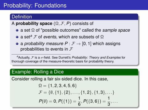
Probability: Foundations

DefinitionA probability space (Ω,F ,P) consists of

a set Ω of "possible outcomes" called the sample spacea seta F of events, which are subsets of Ω

a probability measure P : F → [0,1] which assignsprobabilities to events in F

aActually, F is a σ-field. See Durrett’s Probability: Theory and Examples forthorough coverage of the measure-theoretic basis for probability theory.

Example: Rolling a DiceConsider rolling a fair six-sided dice. In this case,

Ω = 1,2,3,4,5,6F = ∅, 1, 2, . . . , 1,2, 1,3, . . .

P(∅) = 0,P(1) =16,P(3,6) =

13, . . .

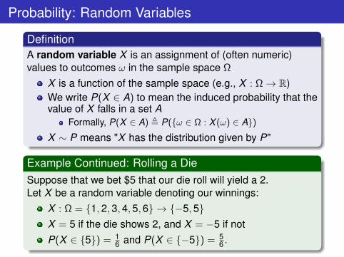
Probability: Random Variables

DefinitionA random variable X is an assignment of (often numeric)values to outcomes ω in the sample space Ω

X is a function of the sample space (e.g., X : Ω→ R)We write P(X ∈ A) to mean the induced probability that thevalue of X falls in a set A

Formally, P(X ∈ A) , P(ω ∈ Ω : X (ω) ∈ A)X ∼ P means "X has the distribution given by P"

Example Continued: Rolling a DieSuppose that we bet $5 that our die roll will yield a 2.Let X be a random variable denoting our winnings:

X : Ω = 1,2,3,4,5,6 → −5,5X = 5 if the die shows 2, and X = −5 if notP(X ∈ 5) = 1

6 and P(X ∈ −5) = 56 .

Probability: Common Discrete Distributions

Common discrete distributions for a random variable X :Bernoulli(p): p ∈ [0,1]; X ∈ 0,1

P(X = 1) = p,P(X = 0) = 1− p

e.g., X = 1 if biased coin comes up heads, 0 otherwise

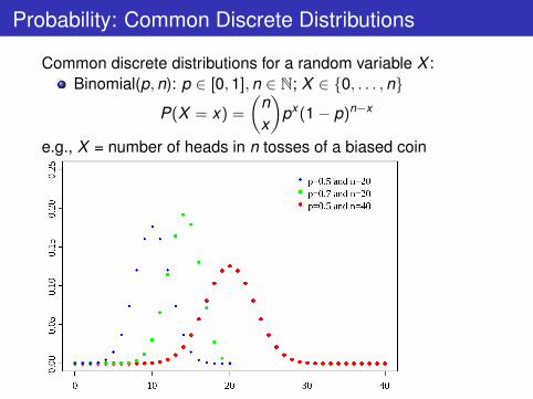
Probability: Common Discrete Distributions

Common discrete distributions for a random variable X :Binomial(p,n): p ∈ [0,1],n ∈ N; X ∈ 0, . . . ,n

P(X = x) =

(nx

)px (1− p)n−x

e.g., X = number of heads in n tosses of a biased coin

Probability: Common Discrete Distributions

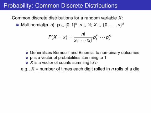
Common discrete distributions for a random variable X :Multinomial(p,n): p ∈ [0,1]k ,n ∈ N; X ∈ 0, . . . ,nk

P(X = x) =n!

x1! · · · xk !px1

1 · · · pxkk

Generalizes Bernoulli and Binomial to non-binary outcomesp is a vector of probabilities summing to 1X is a vector of counts summing to n

e.g., X = number of times each digit rolled in n rolls of a die

Probability: Common Discrete Distributions

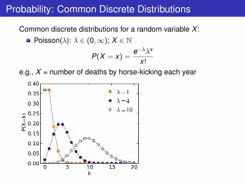
Common discrete distributions for a random variable X :Poisson(λ): λ ∈ (0,∞); X ∈ N

P(X = x) =e−λλx

x!

e.g., X = number of deaths by horse-kicking each year

Probability: From Discrete to Continuous

DefinitionThe probability mass function (pmf) of a discrete randomvariable X is defined as p(x) = P(X = x).

DefinitionThe cumulative distribution function (cdf) of a randomvariable X ∈ Rm is defined for x ∈ Rm as F (x) = P(X ≤ x).

DefinitionWe say that X has a probability density function (pdf) p if wecan write F (x) =

∫ x−∞ p(y)dy .

In practice, the continuous random variables with which wewill work will have densities.For convenience, in the remainder of this lecture we willassume that all random variables take values in somecountable numeric set, R, or a real vector space.

Probability: Common Continuous Distributions

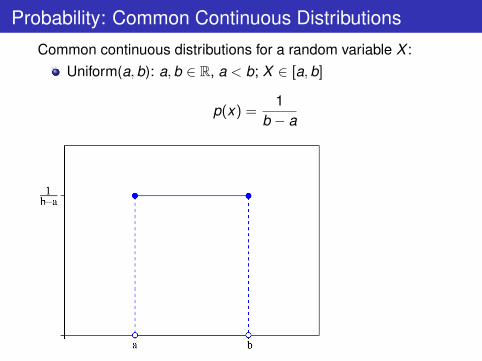
Common continuous distributions for a random variable X :Uniform(a,b): a,b ∈ R, a < b; X ∈ [a,b]

p(x) =1

b − a

Probability: Common Continuous Distributions

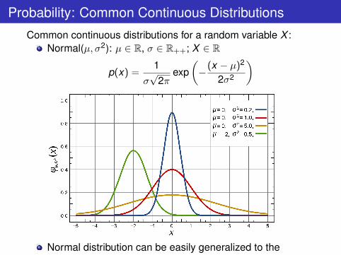
Common continuous distributions for a random variable X :Normal(µ, σ2): µ ∈ R, σ ∈ R++; X ∈ R

p(x) =1

σ√

2πexp

(−(x − µ)2

2σ2

)

Normal distribution can be easily generalized to themultivariate case, in which X ∈ Rm. In this context, µbecomes a real vector and σ is replaced by a covariancematrix.

Probability: Common Continuous Distributions

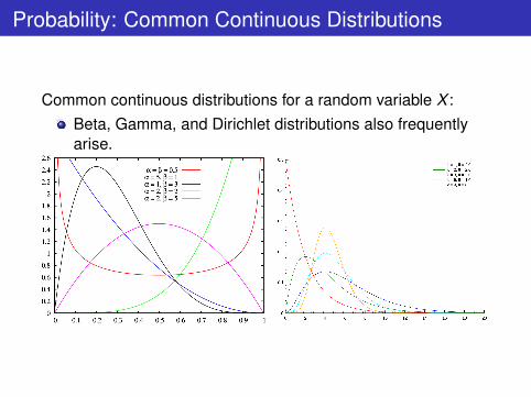
Common continuous distributions for a random variable X :Beta, Gamma, and Dirichlet distributions also frequentlyarise.

Probability: DistributionsOther Distribution Types

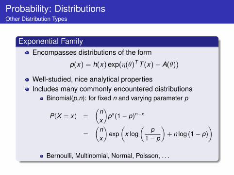
Exponential FamilyEncompasses distributions of the form

p(x) = h(x) exp(η(θ)T T (x)− A(θ))

Well-studied, nice analytical propertiesIncludes many commonly encountered distributions

Binomial(p,n): for fixed n and varying parameter p

P(X = x) =

(nx

)px (1− p)n−x

=

(nx

)exp

(x log

(p

1− p

)+ n log (1− p)

)

Bernoulli, Multinomial, Normal, Poisson, . . .

Probability: Expectation

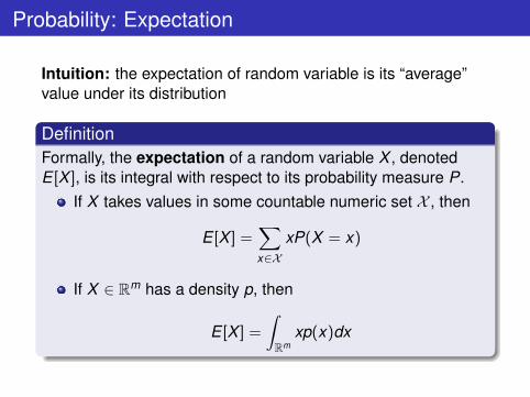
Intuition: the expectation of random variable is its “average”value under its distribution

DefinitionFormally, the expectation of a random variable X , denotedE [X ], is its integral with respect to its probability measure P.

If X takes values in some countable numeric set X , then

E [X ] =∑x∈X

xP(X = x)

If X ∈ Rm has a density p, then

E [X ] =

∫Rm

xp(x)dx

Probability: More on Expectation

Properties of ExpectationExpection is linear: E [aX + b] = aE [X ] + b. Also, if Y isalso a random variable, then E [X + Y ] = E [X ] + E [Y ].Expectation is monotone: if X ≥ Y , then E [X ] ≥ E [Y ]Probabilities are expectations:

Let 1A equal 1 when the event A occurs and 0 otherwiseE [1A] = P(1A = 1)1 + P(1A = 0)0 = P(1A = 1) = P(A)

Expectations also obey various inequalities, includingJensen’s, Cauchy-Schwarz, etc.

VarianceThe variance of a random variable X is defined as

Var(X ) = E [(X − E [X ])2] = E [X 2]− (E [X ])2

and obeys the following for a,b ∈ R:

Var(aX + b) = a2Var(X ).

Probability: Independence

Intuition: two random variables are independent if knowing thevalue of one yields no knowledge about the value of the other

DefinitionFormally, two random variables X and Y are independent,written X ⊥ Y , iff

P(X ∈ A,Y ∈ B) = P(X ∈ A)P(Y ∈ B)

for all (measurable) subsets A and B in the ranges of X and Y .If X ,Y have densities pX (x),pY (y), then they areindependent if

pX ,Y (x , y) = pX (x)pY (y)

for all x , y .

Probability: Conditioning

Intuition: conditioning allows us to capture the probabilisticrelationships between different random variables

DefinitionFor events A and B ∈ F , P(A|B) is the probability that A willoccur given that we know that event B has occurred.

If P(B) > 0, then P(A|B) =P(A ∩ B)

P(B)

Example: Random variables X and Y

P(X ∈ C|Y ∈ D) =P(X ∈ C,Y ∈ D)

P(Y ∈ D)

In terms of densities, p(y |x) =p(x , y)

p(x), for p(x) > 0 where

p(x) =∫

p(x , y)dy .If X and Y are independent, P(X ∈ C|Y ∈ D) = P(X ∈ C).

Probability: More on Conditional Probability

For any events A and B (e.g., we might have A = Y ≤ 5),

P(A ∩ B) = P(A|B)P(B)

Bayes’ Theorem

P(A|B)P(B) = P(A ∩ B) = P(B ∩ A) = P(B|A)P(A)

Equivalently, if P(B) > 0, P(A|B) =P(B|A)P(A)

P(B)

Bayes’ Theorem provides a means of inverting the "order"of conditioning

Probability: Conditional Independence

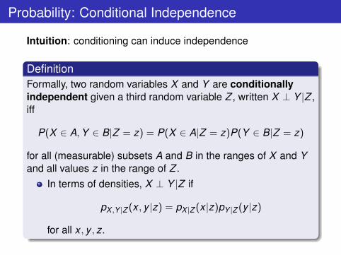
Intuition: conditioning can induce independence

DefinitionFormally, two random variables X and Y are conditionallyindependent given a third random variable Z , written X ⊥ Y |Z ,iff

P(X ∈ A,Y ∈ B|Z = z) = P(X ∈ A|Z = z)P(Y ∈ B|Z = z)

for all (measurable) subsets A and B in the ranges of X and Yand all values z in the range of Z .

In terms of densities, X ⊥ Y |Z if

pX ,Y |Z (x , y |z) = pX |Z (x |z)pY |Z (y |z)

for all x , y , z.

Statistics: Frequentist Basics

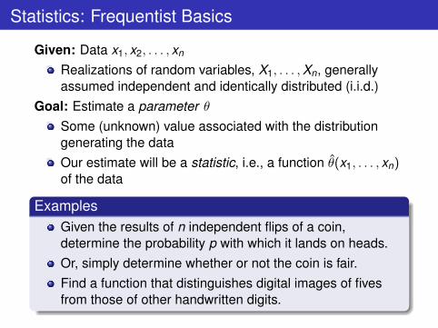
Given: Data x1, x2, . . . , xn

Realizations of random variables, X1, . . . ,Xn, generallyassumed independent and identically distributed (i.i.d.)

Goal: Estimate a parameter θSome (unknown) value associated with the distributiongenerating the dataOur estimate will be a statistic, i.e., a function θ(x1, . . . , xn)of the data

ExamplesGiven the results of n independent flips of a coin,determine the probability p with which it lands on heads.Or, simply determine whether or not the coin is fair.Find a function that distinguishes digital images of fivesfrom those of other handwritten digits.

Statistics: Parameter Estimation

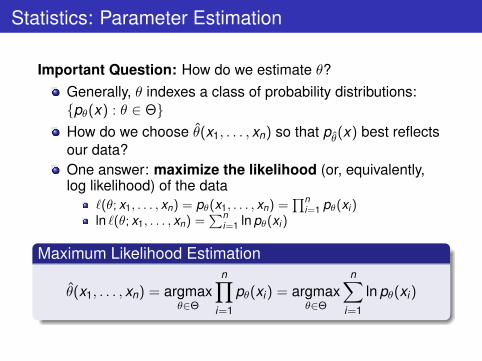
Important Question: How do we estimate θ?Generally, θ indexes a class of probability distributions:pθ(x) : θ ∈ ΘHow do we choose θ(x1, . . . , xn) so that pθ(x) best reflectsour data?One answer: maximize the likelihood (or, equivalently,log likelihood) of the data

`(θ; x1, . . . , xn) = pθ(x1, . . . , xn) =∏n

i=1 pθ(xi )ln `(θ; x1, . . . , xn) =

∑ni=1 ln pθ(xi )

Maximum Likelihood Estimation

θ(x1, . . . , xn) = argmaxθ∈Θ

n∏i=1

pθ(xi) = argmaxθ∈Θ

n∑i=1

ln pθ(xi)

Statistics: Maximum Likelihood EstimationExample: Normal Mean

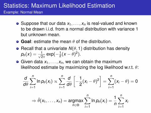
Suppose that our data x1, . . . , xn is real-valued and knownto be drawn i.i.d. from a normal distribution with variance 1but unknown mean.Goal: estimate the mean θ of the distribution.Recall that a univariate N(θ,1) distribution has densitypθ(x) = 1√

2πexp(−1

2(x − θ)2).

Given data x1, . . . , xn, we can obtain the maximumlikelihood estimate by maximizing the log likelihood w.r.t. θ:

ddθ

n∑i=1

ln pθ(xi) ∝n∑

i=1

ddθ

[−1

2(xi − θ)2

]=

n∑i=1

(xi − θ) = 0

⇒ θ(x1, . . . , xn) = argmaxθ∈Θ

n∑i=1

ln pθ(xi) =1n

n∑i=1

xi

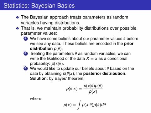
Statistics: Bayesian Basics

The Bayesian approach treats parameters as randomvariables having distributions.That is, we maintain probability distributions over possibleparameter values:

1 We have some beliefs about our parameter values θ beforewe see any data. These beliefs are encoded in the priordistribution p(θ).

2 Treating the parameters θ as random variables, we canwrite the likelihood of the data X = x as a conditionalprobability: p(x |θ).

3 We would like to update our beliefs about θ based on thedata by obtaining p(θ|x), the posterior distribution.Solution: by Bayes’ theorem,

p(θ|x) =p(x |θ)p(θ)

p(x)

wherep(x) =

∫p(x |θ)p(θ)dθ

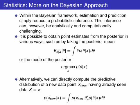
Statistics: More on the Bayesian Approach

Within the Bayesian framework, estimation and predictionsimply reduce to probabilistic inference. This inferencecan, however, be analytically and computationallychallenging.It is possible to obtain point estimates from the posterior invarious ways, such as by taking the posterior mean

Eθ|X [θ] =

∫θp(θ|x)dθ

or the mode of the posterior:

argmaxθ

p(θ|x)

Alternatively, we can directly compute the predictivedistribution of a new data point Xnew, having already seendata X = x :

p(xnew|x) =

∫p(xnew|θ)p(θ|x)dθ

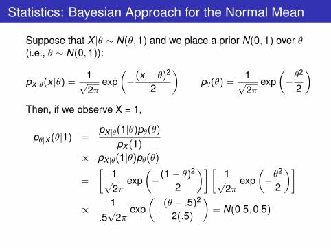
Statistics: Bayesian Approach for the Normal Mean

Suppose that X |θ ∼ N(θ,1) and we place a prior N(0,1) over θ(i.e., θ ∼ N(0,1)):

pX |θ(x |θ) =1√2π

exp(−(x − θ)2

2

)pθ(θ) =

1√2π

exp(−θ

2

2

)Then, if we observe X = 1,

pθ|X (θ|1) =pX |θ(1|θ)pθ(θ)

pX (1)

∝ pX |θ(1|θ)pθ(θ)

=

[1√2π

exp(−(1− θ)2

2

)][1√2π

exp(−θ

2

2

)]∝ 1

.5√

2πexp

(−(θ − .5)2

2(.5)

)= N(0.5,0.5)

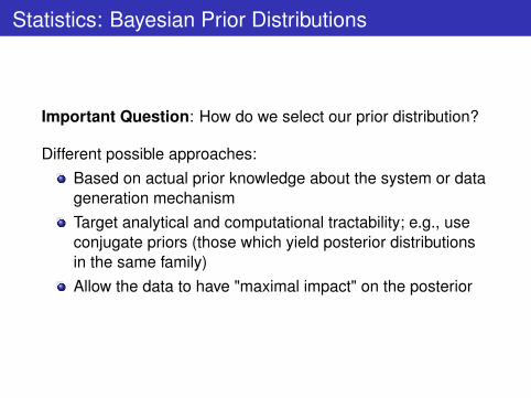
Statistics: Bayesian Prior Distributions

Important Question: How do we select our prior distribution?

Different possible approaches:Based on actual prior knowledge about the system or datageneration mechanismTarget analytical and computational tractability; e.g., useconjugate priors (those which yield posterior distributionsin the same family)Allow the data to have "maximal impact" on the posterior

Statistics: Parametric vs. Non-Parametric Models

All of the models considered so far are parametricmodels: they are determined by a fixed, finite number ofparameters.This can limit the flexibility of the model.Instead, can permit a potentially infinite number ofparameters which is allowed to grow as we see more data.Such models are called non-parametric.Although non-parametric models yield greater modelingflexibility, they are generally statistically andcomputationally less efficient.

Statistics: Generative vs. Discriminative Models

Suppose that, based on data (x1, y1), . . . , (xn, yn), wewould like to obtain a model whereby we can predict thevalue of Y based on an always-observed random variableX .Generative Approach: model the full joint distributionP(X ,Y ), which fully characterizes the relationship betweenthe random variables.Discriminative Approach: only model the conditionaldistribution P(Y |X )

Both approaches have strengths and weaknesses and areuseful in different contexts.

Linear Algebra: Basics

Matrix TransposeFor an m × n matrix A with (A)ij = aij , its transpose is ann ×m matrix AT with (AT )ij = aji .(AB)T = BT AT

Matrix InverseThe inverse of a square matrix A ∈ Rn×n is the matrix A−1

such that A−1A = I.This notion generalizes to non-square matrices via left-and right-inverses.Not all matrices have inverses.If A and B are invertible, then (AB)−1 = B−1A−1.Computation of inverses generally requires O(n3) time.

Linear Algebra: Basics

TraceFor a square matrix A ∈ Rn×n, its trace is defined astr(A) =

∑ni=1(A)ii .

tr(AB) = tr(BA)

Eigenvectors and EigenvaluesGiven a matrix A ∈ Rn×n, u ∈ Rn\0 is called aneigenvector of A with λ ∈ R the corresponding eigenvalue if

Au = λu

An n × n matrix can have no more than n distincteigenvector/eigenvalue pairs.

Linear Algebra: Basics

More definitionsA matrix A is called symmetric if it is square and(A)ij = (A)ji ,∀i , j .A symmetric matrix A is positive semi-definite (PSD) if allof its eigenvalues are greater than or equal to 0.Changing the above inequality to >, ≤, or < yields thedefinitions of positive definite, negative semi-definite, andnegative definite matrices, respectively.A positive definite matrix is guaranteed to have an inverse.

Linear Algebra: Matrix Decompositions

Eigenvalue DecompositionAny symmetric matrix A ∈ Rn×n can be decomposed as follows:

A = UΛUT

where Λ is a diagonal matrix with the eigenvalues of A on itsdiagonal, U has the corresponding eigenvectors of A as itscolumns, and UUT = I.

Singular Value DecompositionAny matrix A ∈ Rm×n can be decomposed as follows:

A = UΣV T

where UUT = VV T = I and Σ is diagonal.

Other Decompositions: LU (into lower and upper triangularmatrices); QR; Cholesky (only for PSD matrices)

Optimization: Basics

We often seek to find optima (minima or maxima) of somereal-valued vector function f : Rn → R. For example, wemight have f (x) = xT x .Furthermore, we often constrain the value of x in someway: for example, we might require that x ≥ 0.In standard notation, we write

minx∈X

f (x)

s.t. gi(x) ≤ 0, i = 1, . . . ,Nhi(x) = 0, i = 1, . . . ,M

Every such problem has a (frequently useful)corresponding Lagrange dual problem which lower-boundsthe original, primal problem and, under certain conditions,has the same solution.It is only possible to solve these optimization problemsanalytically in special cases, though we can often findsolutions numerically.

Optimization: A Simple Example

Consider the following unconstrained optimization problem:

minx∈Rn

‖Ax − b‖22 = minx∈Rn

(Ax − b)T (Ax − b)

In fact, this is the optimization problem that we must solveto perform least-squares regression.To solve it, we can simply set the gradient of the objectivefunction equal to 0.The gradient of a function f (x) : Rn → R is the vector ofpartial derivatives with respect to the components of x :

∇x f (x) =

(∂f∂x1

, . . .∂f∂xn

)

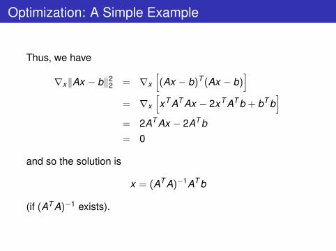
Optimization: A Simple Example

Thus, we have

∇x‖Ax − b‖22 = ∇x

[(Ax − b)T (Ax − b)

]= ∇x

[xT AT Ax − 2xT AT b + bT b

]= 2AT Ax − 2AT b= 0

and so the solution is

x = (AT A)−1AT b

(if (AT A)−1 exists).

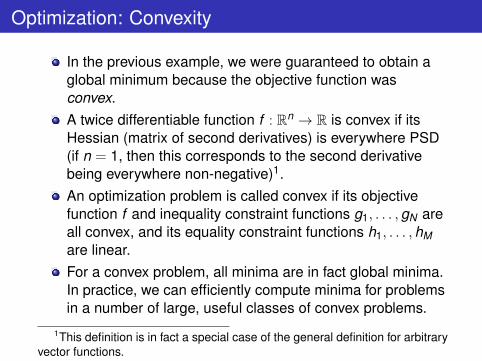
Optimization: Convexity

In the previous example, we were guaranteed to obtain aglobal minimum because the objective function wasconvex.A twice differentiable function f : Rn → R is convex if itsHessian (matrix of second derivatives) is everywhere PSD(if n = 1, then this corresponds to the second derivativebeing everywhere non-negative)1.An optimization problem is called convex if its objectivefunction f and inequality constraint functions g1, . . . ,gN areall convex, and its equality constraint functions h1, . . . ,hMare linear.For a convex problem, all minima are in fact global minima.In practice, we can efficiently compute minima for problemsin a number of large, useful classes of convex problems.

1This definition is in fact a special case of the general definition for arbitraryvector functions.