Continuity, Inertia and ε-Equilibrium:

A Test of the Theory of Continuous Time Games

Evan Calford Ryan Oprea∗

August 27, 2015

Abstract

The theory of continuous time games (Simon and Stinchcombe (1989), Bergin and MacLeod

(1993)) shows that continuous time interactions can generate very different equilibrium behavior

than conventional discrete time interactions. We introduce new laboratory methods that allow

us to eliminate natural inertia in subjects’ decisions in continuous time experiments, thereby

satisfying critical premises of the theory and enabling a first-time direct test. Applying these new

methods to a simple diagnostic timing game we find strikingly large gaps in behavior between

discrete and continuous time as the theory suggests. Reintroducing natural inertia into these

games causes continuous time behavior to collapse to discrete-time like levels in some settings

as predicted by Nash. However, contra Nash, the strength of this effect is fundamentally shaped

by the severity of inertia: behavior tends towards discrete time benchmarks as inertia grows

large and perfectly continuous time benchmarks is it falls towards zero.

Keywords: Dynamic Games, Continuous Time, Laboratory Experiments, Game Theory,

Epsilon Equilibrium

JEL codes: C73, C92, D01, and C72

1 Introduction

In game theory models, players usually make decisions in lock-step at a predetermined set of dates

– a timing protocol we will call “Perfectly Discrete time.” Most real world interaction, by contrast,

∗Calford: Economics Department, University of British Columbia, Vancouver, BC, V6T 1Z4, evancal-

ford@gmail.com; Oprea: Economics Department, University of California, Santa Barbara, Santa Barbara, CA, 95064,

roprea@gmail.com.

1

unfolds asynchronously in unstructured continuous time, perhaps with some inertia delaying mutual

response. Does this difference between typical modeling conventions and real-world interactions

matter? Theoretical work on the effects of continuous time environments on behavior (developed

especially in Simon and Stinchcombe (1989) and Bergin and MacLeod (1993)) focuses on what we

will call “Perfectly Continuous time,” a limiting case in which players can respond instantly (that

is with zero inertia) to one another, and arrives at a surprising answer: Perfectly Discrete time and

Perfectly Continuous time can often support fundamentally different equilibria, resulting in wide

gaps in behavior between the two settings.

In this paper we introduce new techniques that allow us to evaluate these theorized gaps in

the laboratory directly and assess their relevance for understanding real world behavior. We pose

two main questions. First, does the gulf between Perfectly Discrete and Perfectly Continuous

time suggested by the theory describe real human behavior? Though equilibria exist that produce

large differences in behavior (and authors such as Simon and Stinchcombe (1989) argue that these

equilibria should be considered highly focal), multiplicity of equilibrium in Perfectly Continuous

time means that the effect of continuous time is, ultimately, theoretically indeterminate. Second, we

ask how empirically relevant these gaps are: can more realistic, imperfectly continuous time games

(games with natural, positive inertia that we call “Inertial Continuous time” games) generate

Perfectly Continuous-like outcomes? Strict Nash suggests not but, as Simon and Stinchcombe

(1989) and Bergin and MacLeod (1993) emphasize, even slight deviations from Nash assumptions

(ala ε-equilibrium) allow Perfectly Continuous-like behavior to survive as equilibria in the face of

inertia, provided inertia is sufficiently small.

Recent experiments have begun to investigate the relationship between continuous and discrete

time behavior in the lab (e.g. Friedman and Oprea (2012) and Bigoni et al. (2015))1 but have

not yet directly tested the theory motivating these questions for a simple reason: natural human

reaction lags in continuous time settings generate inertia that prevents a direct implementation of

the premises of the theory. These Inertial Continuous time settings are empirically important (and

1Both Friedman and Oprea (2012) and Bigoni et al. (2015) report evidence from prisoner’s dilemmas played with

flow payoffs in Inertial Continuous time (i.e. subjects in these experiments suffer natural reaction lags that prevent

instant response to the actions of others). While the Friedman and Oprea (2012) design varies the continuity of

the environment (discrete vs. continuous time interaction) in deterministic horizon games, the Bigoni et al. (2015)

design centers on varying the stochasticity of the horizon (deterministic vs. stochastic horizon) in continuous time

games. Other more distantly related continuous time papers include experimental work on multi-player centipede

games (Murphy et al. 2006), public-goods games (Oprea et al. (2014)), network games (Berninghaus et al. (2006)),

minimum-effort games (Deck and Nikiforakis (2012)), hawk-dove games (Oprea et al. (2011)) and the effects of public

signals (Evdokimov and Rahman (2014)).

2

of independent interest) but are insufficient for a direct theory test because they generate very

different equilibrium behavior from the Perfectly Continuous time environments that anchor the

theory (a prediction we test and find strong though highly qualified support for in our data). In our

experimental design, we introduce a new protocol (“freeze time”) that eliminates inertia by pausing

the game for several seconds after subjects make decisions, allowing them to respond “instantly” to

actions of others (i.e. with no lag in game time) and thus allowing us to test Perfectly Continuous

predictions. By systematically comparing behavior in this Perfectly Continuous setting to both

Perfectly Discrete time and Inertial Continuous time settings we are able to pose and answer our

motivating questions.

We apply this new methodology to a simple timing game similar to one discussed in Simon and

Stinchcombe (1989) that is ideally suited for a careful test of the theory.2 In this game, each of

two agents decides independently when to enter a market. Joint delay is mutually beneficial up to

a point, but agents benefit from preempting their counterparts (and suffer by being preempted).

In Perfectly Discrete time, agents will enter the market at the very first opportunity, sacrificing

significant potential profits in subgame perfect equilibrium. By contrast, in Perfectly Continuous

time, agents can, in equilibrium, delay entry until 40% of the game has elapsed, thereby maximiz-

ing joint profits.3(Simon and Stinchcombe (1989) emphasize this equilibrium and point out that it

uniquely survives iterated elimination of weakly dominated strategies, but many other equilibria

– including inefficient immediate-entry equilibrium – exist in Perfectly Continuous time.) Impor-

tantly, Inertial Continuous time of the sort studied in previous experiments leads not to Perfectly

Continuous time-like multiplicity in equilibrium but only to the inefficient instant entry predicted

for Perfectly Discrete time – as Bergin and MacLeod (1993) point out even a small amount of inertia

theoretically erases all of the efficiency enhancing potential of continuous time in Nash equilibrium.

In the first part of our experimental design we pose our main question by comparing Perfectly

Discrete and Perfectly Continuous time using a Baseline set of parameters and 60 second runs of the

game. In the Perfectly Discrete time protocol, we divide the 60 second game into 16 discrete grid

2Compared to, for instance, the continuously repeated prisoner’s dilemma (PD), our timing game has several

advantages for a diagnostic test. First, the joint profit maximizing outcome predicted by Simon and Stinchcombe

(1989) is interior, meaning simple heuristics like “cooperate until the end of the game” cannot be confused with

Nash play. Second, the strategy space is considerably simpler than the PD, making measurement of decisions and

inferences about strategies crisper (while simplifying the ε-equilibrium set considerably). Finally, the PD frames the

contrast between cooperation and defection somewhat starkly and may therefore trigger social behaviors that have

little to do with the forces we designed our experiment to study – we speculated in designing the experiment that

our timing game would be somewhat cleaner from this perspective.3More precisely, the agents are maximizing joint profits subject to playing non-strictly dominated strategies.

3

points and allow subjects to simultaneously choose at each grid point whether to enter the market.

In the Perfectly Continuous time protocol we instead allow subjects to enter at any moment but,

crucially, eliminate natural human inertia by freezing the game after any player enters, allowing

her counterpart to enter “immediately” from a game-time perspective if she enters during the

ample window of the freeze. We find evidence of large and extremely consistent differences in

behavior across these two protocols. Virtually all subjects in the Perfectly Discrete time treatment

suboptimally enter at the first possible moment while virtually all subjects in Perfectly Continuous

time enter 40% of the way into the period, forming a tight mode around the joint profit maximizing

entry time. The results thus support the conjecture of a large - indeed, from a payoff perspective,

maximally large – gap between Perfectly Continuous and Discrete time behaviors.

In the second part of the design, we study how introducing realistic inertia into continuous time

interaction changes the nature of the results observed in our Perfectly Continuous time treatment.

Though strict Nash predicts that even a tiny amount of inertia will force behavior back to Per-

fectly Discrete-like immediate entry times, alternatives such as ε-equilibrium suggest that Perfectly

Continuous-like results may survive as equilibria at low levels of inertia. In Inertial Continuous

time treatments we replicate our Perfectly Continuous time treatment but remove the freeze time

protocol, thereby allowing natural human reaction lags to produce a natural source of inertia. We

systematically vary the severity of this inertia by varying the speed of the game relative to sub-

jects’ natural reaction lags and find that when inertia is highest, entry times collapse to zero in

continuous time as predicted by Nash. However when we lower inertia to sufficiently small levels,

we observe large entry delays that are nearly as efficient as those observed in Perfectly Continuous

time. Thus, realistic Inertial Continuous Time behavior is well approximated by the extreme of

Perfectly Discrete time when inertia is large and better approximated by the extreme of Perfectly

Continuous time when inertia is small. While these patterns are inconsistent with Nash, they are,

as both Simon and Stinchcombe (1989) and Bergin and MacLeod (1993) stress, consistent with

ε-equilibrium.4

We close the paper by showing that ε-equilibrium, which anticipates behavior so well in Inertial

Continuous, also outperforms Nash in organizing Perfectly Discrete and Perfectly Continuous time

behavior. We test a distinctive comparative static prediction of ε-equilibrium that is uniquely

testable using our Perfectly Discrete and Perfectly Continuous time protocols. By lowering a payoff

parameter in the timing game we can reduce the rate at which subjects increase their earnings

4ε-equilibrium has also had success in organizing results ex post in closely related experimental work (in particular

Friedman and Oprea (2012)) Posing strong ex ante tests for this alternative to Nash was a major design goal of this

experiment.

4

by preempting a counterpart. This change can have a crucial effect on the ε-equilibrium set in

Perfectly Discrete time but should have no corresponding effect in Perfectly Continuous time (it

should have no effect on either treatment in Nash equilibrium). We find the exact pattern predicted

by ε-equilibrium in the data: lowering the preemption temptation leads most subjects to abandon

immediate entry in Perfectly Discrete time but causes no change in behavior Perfectly Continuous

time. The data thus, overall, provides strong evidence that ε-equilibrium is an important organizing

concept for this class of game.

The results of our experiment suggest a role for Perfectly Continuous time theoretical bench-

marks in predicting and interpreting real-world behavior, even if the world is never perfectly con-

tinuous. Changes in technology have recently narrowed – and continue to narrow – the gap between

many types of human interactions and the Perfectly Continuous setting described in the theory.

Constant mobile access to markets and social networks, the proliferation of applications that speed

up search and the advent of automated agents deployed for trade and search have the effect of

reducing inertia in human interactions. Our results suggest, contra Nash, that such movements to-

wards continuity may generate some of the dramatic effects on behavior predicted for (and observed

in) Perfectly Continuous time even if inertia never falls quite to zero. Guided by these results, we

conjecture that the share of interactions that are better understood through the theoretical lens of

Perfectly Continuous time than that of Perfectly Discrete time will grow as social and economic

activity continues to be transformed by this sort of technological change.

The remainder of the paper is organized as follows. Section 2 gives an overview of the main

relevant theoretical results and section 3 describes the experimental design. Section 4 presents our

results and Section 5 provides a discussion of the results and concludes the paper. Appendices

collect theoretical proofs and the instructions to subjects.

2 Theoretical Background and Hypotheses

In section 2.1 we introduce our timing game and in section 2.2 we state and discuss a set of

propositions characterizing Nash equilibrium and providing us with our main hypotheses. In section

2.3 we consider alternative hypotheses motivated by ε-equilibrium.

5

2.1 A Diagnostic Timing Game

Consider the following simple timing game, adapted from one described in Simon and Stinchcombe

(1989). Two firms, i ∈ {a, b}, each choose a time ti ∈ [0, 1] at which to enter a market, perhaps

conditioning this choice on the history of the game.5 Payoffs depend on the order of entry according

to the following symmetric function:

Ua(ta, tb) =

1−tb

2

[ΠD + (tb − ta)(1 + 2

1−tb )ΠF

]− c(1− ta)2 if ta < tb

1−ta2 ΠD − c(1− ta)2 if ta = tb

1−ta2 [ΠD − (ta − tb)ΠS ]− c(1− ta)2 if tb < ta

(1)

with parameters assumed to satisfy 0 < 2c < ΠS ≤ ΠD < 4c and 4c3 ≤ ΠF ≤ 4c. Though the

applied setting modeled by this sort of game matters little for our relatively abstract experiment,

we can interpret the model as one in which firms face quadratic costs for time spent in the market

(parameterized by c), earn a duopoly flow profit rate of ΠD while sharing the market, earn a greater

flow profit ΠF while a monopolist and suffer a permanent reduced earnings rate (parameterized by

ΠS) proportional to the time one’s counterpart has spent as a monopolist.

Several characteristics of this game are particularly important for what follows. First, firms earn

identical profits if they enter at the same time and this simultaneous entry payoff is strictly concave

in entry time, reaching a maximum at a time t∗ = 1 − ΠD4c ∈ (0, 1

2). Second, if one of the firms

instead enters earlier than the other (at time t′), she earns a higher payoff and her counterpart

a lower payoff than had they entered simultaneously at time t′. The firms thus maximize joint

earnings by delaying entry until an interior time t∗ but at each moment each firm has a motivation

to preempt its counterpart and to avoid being preempted.

2.2 Discrete, Inertial and Perfectly Continuous Time Predictions

What entry times can be supported as equilibria in this game? The key observation motivating both

the theory and our experiment is that the answer depends on how time operates in the game. In

this subsections we characterize equilibrium under three distinct protocols: Perfectly Discrete time,

5To conserve notation, we normalize the length of the game to be 1 for the theoretical analysis. In our experiment,

we sometimes vary the length of the game (and with it the severity of inertia and predicted time of entry) across

treatments.

6

Perfectly Continuous time and Inertial Continuous time (here we only sketch the main conceptual

issues, deferring technical discussion to Appendix A).

We begin with Perfectly Discrete time, the simplest and most familiar case. Here, time is

divided into G + 1 evenly spaced grid points (starting always at t = 0) on [0, 1] and players

make simultaneous decisions at each of these points. More precisely, each player chooses a time

t ∈ {0, 1/G, ..., (G − 1)/G, 1} at which to enter, possibly conditioning this choice on the history

of the game, Ht at each grid point. Earnings are given by equation 1 applied to the dates on

the grid at which entry occurred.6 As in familiar dynamic discrete time games like the centipede

game and the finitely repeated prisoner’s dilemma there is a tension here between efficiency (which

requires mutual delay until at least the grid point immediately prior to t∗) and individual sequential

rationality (which encourages a player to preempt her counterpart). Applying the logic of backwards

induction, strategies that delay entry past the first grid point unravel, leaving immediate entry at

the first grid point, t = 0, as the unique subgame perfect equilibrium, regardless of G.

Proposition 1. In Perfectly Discrete time, the unique subgame perfect equilibrium is for both firms

to enter at time 0, regardless of the fineness of the grid, G.

Proof. : See Appendix A.1.1.

At the opposite extreme, in Perfectly Continuous time players are not confined to a grid of entry

times but can instead enter at any moment ti ∈ [0, 1] (again, possibly conditioning on the history

of the game at each t, Ht). Simon and Stinchcombe (1989) emphasize the relationship between the

two extremes, modeling Perfectly Continuous Time as the limit of a Perfectly Discrete time game as

G approaches infinity. In this limit, players can respond instantly to entry choices made by others:

if an agent enters the market at time t her counterpart can respond by also entering at t, moving

in response to her counterpart but at identical dates. Since, in our game, delaying entry after a

counterpart enters is strictly payoff decreasing, no player can expect to succeed in preempting her

counterpart (or have reason to fear being preempted). This elimination of preemption motives also

protects efficient delayed entry from unravelling and thus makes it possible to support any entry

time t ∈ [0, t∗] as an equilibrium.7

6For example, if firm a entered at the third grid point, and firm b entered at the fifth grid point, the payoff for

firm a is given by Ua( 2G, 4G

).7Entry times greater than t∗ cannot be supported in equilibrium because they are always payoff dominated by

t∗. Notice that despite the symmetry of the (joint entry) payoff function around t∗, the equilibrium entry set is not

symmetric around t∗ because of the temporal nature of the game.

7

Proposition 2. In Perfectly Continuous time, any entry time t ∈ [0, t∗] can be supported as a

subgame perfect equilibrium outcome.

Proof. We provide three proofs of this proposition. Appendix A.1.2 includes both a self-contained

heuristic proof and a more formal proof that draws directly from Simon and Stinchcombe (1989).

Appendix A.1.3 contains an alternative proof that instead follows the modeling approach of Bergin

and MacLeod (1993).

Though it is possible for Perfectly Discrete and Perfectly Continuous behaviors to radically differ

in equilibrium, this is hardly guaranteed. Because of multiplicity, Perfectly Continuous behavior

may be quite different or quite similar to Perfectly Discrete behavior in equilibrium (t = 0 and t∗

are both supportable in equilibrium in Perfectly Continuous time) depending on the principle of

equilibrium selection at work. This multiplicity is in fact a central motivation for studying these

environments in the laboratory. Simon and Stinchcombe (1989) emphasize that t∗ is the unique

entry time to survive iterated elimination of weakly dominated strategies in our game and they

argue that this refinement is natural in the context of Perfectly Continuous time games. Evaluating

the organizing power of this refinement is another central motivation for our study.

Remark 1. In Perfectly Continuous time, joint entry at t∗ = 1 − ΠD4c is the only outcome that

survives iterated elimination of weakly dominated strategies.

Proof. A heuristic proof is provided in appendix A.1.2. For further details, see Simon and Stinch-

combe (1989).

Finally, Inertial Continuous time lies between the extremes of Perfectly Discrete and Perfectly

Continuous time, featuring characteristics of each. Here, as in Perfectly Continuous time, players

can make asynchronous decisions and are not confined to entering at a predetermined grid of times.

However, as in Perfectly Discrete time, players are unable to respond instantly to entry decisions by

their counterparts. In Inertial Continuous time, inability to instantly respond is due to what Bergin

and MacLeod (1993) call inertia (here, simply response lags of exogenous size δ).8 9 With inertial

reaction lags, the logic of unravelling returns as players once again have motives to preempt one

another. As a result, the efficient delayed entry supported in equilibrium in Perfectly Continuous

8Though, in the context of our experiment, inertia simply refers to natural human reaction lags, Bergin and

MacLeod (1993) point out that more general types of inertia are possible.9Throughout the paper we define inertia δ as the ratio of an agent’s reaction lag, δ0, to the total length of the

game, T (i.e. δ ≡ δ0/T ). Inertia is thus the fraction of the game that elapses before an agent can respond to her

counterpart.

8

time evaporates with even an arbitrarily small amount of inertia. Theoretically then, even a tiny

amount of inertia pushes continuous time behavior to Perfectly Discrete levels.

Proposition 3. In Inertial Continuous time, only entry at time 0 can be supported as a subgame

perfect equilibrium regardless of the size of inertia, δ > 0.

Proof. See Appendix A.1.3.

Instead of modeling Perfectly Continuous time as a limit of Perfectly Discrete time as the grid

becomes arbitrarily fine as Simon and Stinchcombe (1989) do, Bergin and MacLeod (1993) model

it as the limit of Inertial Continuous time as inertia approaches zero.10 This alternative method

for defining Perfectly Continuous time leads to an identical equilibrium set to the one described by

Simon and Stinchcombe (1989) for our game.

2.3 Alternative Hypothesis: ε-equilibrium

These Nash results suggest not only that continuous time can fundamentally change behavior but

that this effect will be extremely fragile: even a slight amount of inertia will eliminate any pro-

cooperative effects of continuous time interaction. Since inertia is realistic, this frailty in turn calls

into question the usefulness of the theory for predicting and interpreting behavior in the real-world.

Perhaps for this reason both Simon and Stinchcombe (1989) and Bergin and MacLeod (1993)

motivate the theory of continuous time explicitly with reference to the more forgiving solution

concept of ε-equilibrium, emphasizing that any Perfectly Continuous time Nash equilibrium is

arbitrarily close to some ε-equilibrium of a continuous time game with inertia (and vice versa).11

This means that if agents are willing to tolerate small deviations from best response, they can

support Perfectly Continuous-like outcomes as equilibria even in the face of inertia, provided inertia

is sufficiently small.

The central role ε-equilibrium plays in motivating the theory and connecting it to real-world

settings makes it a natural source of alternative hypotheses for our experiment.12 Under the

10As we point out in Appendix A, while Bergin and MacLeod (1993) assume the strategy space to be constant, we

do not allow re-entry in our experiment. This implies that the strategy space shrinks from two strategies to one after

entry. In our adaptation of Bergin and MacLeod (1993) in Appendix A.1.3, we can reconcile the two approaches by

simply assuming that the size of inertia rises to the remaining length of the game after all histories in which an agent

enters, preventing agents from re-entering.11More precisely, Simon and Stinchcombe (1989) make this same point with respect to synchronous, discrete time

games with very fine time grids.12 Radner’s original motivation for formulating ε-equilibrium (Radner (1980)) is the observation that, in games

9

hypothesis of ε-equilibrium the effect of inertia is not fixed (as it is under the hypothesis of Nash)

but instead depends on the magnitude of inertia. In Inertial Continuous time, when inertia is large,

ε-equilibrium coincides with Nash, supporting only instant entry at t = 0 and mirroring Perfectly

Discrete time Nash outcomes. However when inertia falls below a threshold level (determined by

ε) the equilibrium set expands to support any entry time t ∈ [0, t∗], instead mirroring Perfectly

Continuous time Nash outcomes. Thus ε-equilibrium suggests that Inertial Continuous time can

look much like Perfectly Discrete or Perfectly Continuous time depending on the severity of inertia.

We formalize this in the following proposition:

Proposition 4. Consider a game in inertial continuous time. For any ε > 0, there exists a level

of inertia, δ, small enough to admit any entry time in [0, t∗] in a subgame perfect ε-equilibrium.

For any 0 < ε ≤ ε̂ where

ε̂ =

(

3ΠF4c − 1

)2c if ΠF ≤ 8c

3

3ΠF2 − 3c if ΠF >

8c3

there exists a level of inertia, δ, large enough to admit only entry at t = 0 as the unique subgame

perfect ε-equilibrium.

Proof. See Appendix A.2.2.

ε is unobservable directly, so we test this prediction against the Nash alternative in section 3.2

by varying inertia quite widely across three levels. We calibrated these inertia levels so that, unless

the distribution of ε is very extreme, ε-equilibrium predicts differences in behavior between the

highest and lowest inertias.

Our main interest in ε-equilibrium is in its potential to bridge Inertial Continuous and Perfectly

Continuous behavior. However, we close the design and paper with a diagnostic test of ε-equilibrium

that is rooted in its asymmetric hypothesized effects on Perfectly Continuous and Perfectly Discrete

protocols. This test is based on a simple comparative static, identified in proposition 5: reducing

the temptation to preempt (parameterized by ΠF in equation (1)) sufficiently will have an effect

on ε-equilibrium behavior in Perfectly Discrete time but cause no change in behavior in Perfectly

such as ours, the downside risks and upside rewards from deviating from Nash by delaying entry vanish relative to the

potential rewards from mutual delay as the grid becomes fine or inertia becomes small. ε-equilibrium hypothesizes

that agents may therefore be willing to tolerate small deviations from best response in order to improve their odds

of achieving these sorts of cooperative payouts. Our motivation for studying this alternative hypothesis is strongly

tied to this intuition.

10

Continuous time. By contrast, under the hypothesis of Nash, this change in parameters will have

no effect on behavior under either protocol.

Proposition 5. If ε > 0, a reduction in ΠF will weakly enlarge the set of entry times supportable

in subgame perfect ε-equilibrium in Perfectly Discrete time. However an identical reduction will

have no effect in Perfectly Continuous time.

Proof. See Appendix A.2.2.

Again, we calibrated our change to ΠF (in treatments reported in section 4.3) to be large enough

so that ε-equilibrium predicts an effect for all but the most extreme values of ε.

In Appendix A.2 we prove a set of propositions fully characterizing the ε-equilibrium sets for

our protocols and in Appendix A.2.2 provide proofs of the propositions contained in this subsection.

3 Design and Implementation

In section 3.1 we discuss our strategy for implementing our three timing protocols in the lab and

present the experimental software we built to carry out this strategy. In section 3.2 we present our

treatment design.

3.1 Timing Protocols and Experimental Software

We ran our experiment using a custom piece of software programmed in Redwood (Pettit et al.

(n.d.)). Figures 1 and 2 show screenshots. Using this software, we implemented the three timing

protocols described in Section 2 as follows:

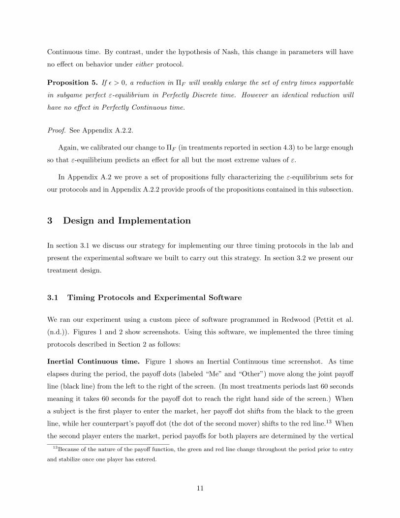
Inertial Continuous time. Figure 1 shows an Inertial Continuous time screenshot. As time

elapses during the period, the payoff dots (labeled “Me” and “Other”) move along the joint payoff

line (black line) from the left to the right of the screen. (In most treatments periods last 60 seconds

meaning it takes 60 seconds for the payoff dot to reach the right hand side of the screen.) When

a subject is the first player to enter the market, her payoff dot shifts from the black to the green

line, while her counterpart’s payoff dot (the dot of the second mover) shifts to the red line.13 When

the second player enters the market, period payoffs for both players are determined by the vertical

13Because of the nature of the payoff function, the green and red line change throughout the period prior to entry

and stabilize once one player has entered.

11

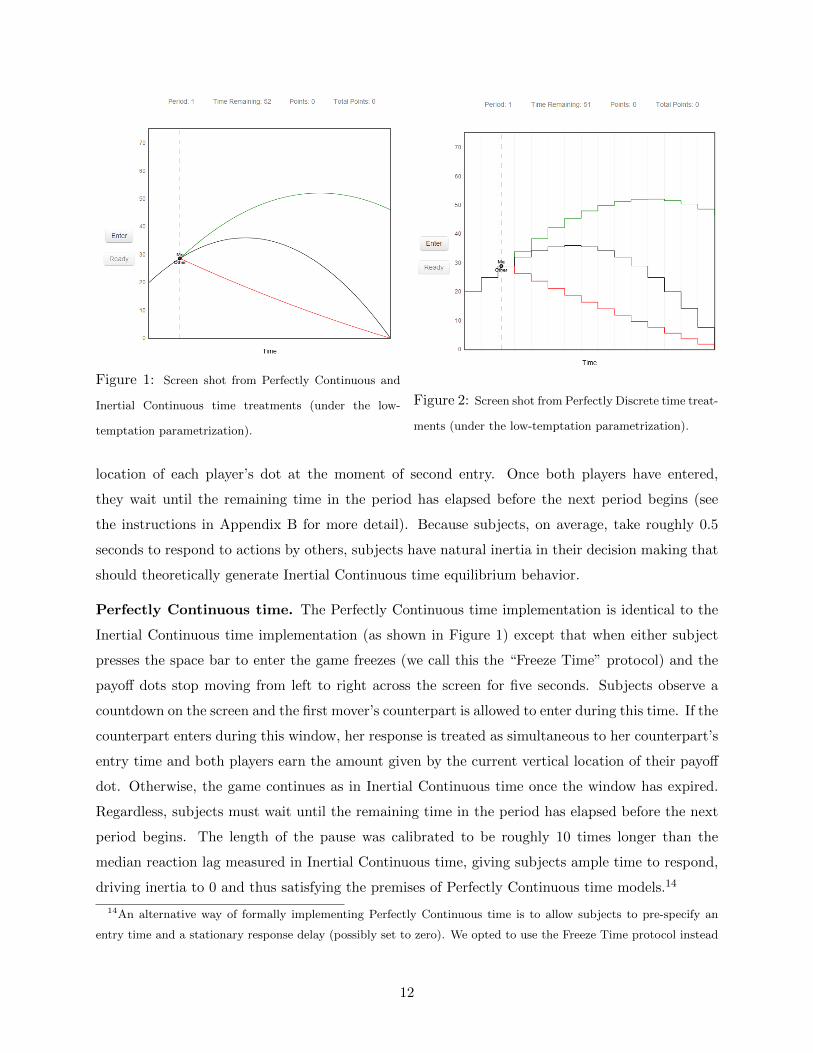
Figure 1: Screen shot from Perfectly Continuous and

Inertial Continuous time treatments (under the low-

temptation parametrization).

Figure 2: Screen shot from Perfectly Discrete time treat-

ments (under the low-temptation parametrization).

location of each player’s dot at the moment of second entry. Once both players have entered,

they wait until the remaining time in the period has elapsed before the next period begins (see

the instructions in Appendix B for more detail). Because subjects, on average, take roughly 0.5

seconds to respond to actions by others, subjects have natural inertia in their decision making that

should theoretically generate Inertial Continuous time equilibrium behavior.

Perfectly Continuous time. The Perfectly Continuous time implementation is identical to the

Inertial Continuous time implementation (as shown in Figure 1) except that when either subject

presses the space bar to enter the game freezes (we call this the “Freeze Time” protocol) and the

payoff dots stop moving from left to right across the screen for five seconds. Subjects observe a

countdown on the screen and the first mover’s counterpart is allowed to enter during this time. If the

counterpart enters during this window, her response is treated as simultaneous to her counterpart’s

entry time and both players earn the amount given by the current vertical location of their payoff

dot. Otherwise, the game continues as in Inertial Continuous time once the window has expired.

Regardless, subjects must wait until the remaining time in the period has elapsed before the next

period begins. The length of the pause was calibrated to be roughly 10 times longer than the

median reaction lag measured in Inertial Continuous time, giving subjects ample time to respond,

driving inertia to 0 and thus satisfying the premises of Perfectly Continuous time models.14

14An alternative way of formally implementing Perfectly Continuous time is to allow subjects to pre-specify an

entry time and a stationary response delay (possibly set to zero). We opted to use the Freeze Time protocol instead

12

Perfectly Discrete time. Figure 2, shows a screen shot for the Perfectly Discrete treatments,

which is very similar to the continuous time screen but for a few changes. First, periods are divided

into G = 15 subperiods, which begin at gridpoints t = {0, 4, 8, ..., 56} (measured in seconds)15,

each marked by a vertical gray line on the subject’s screen. Instead of moving smoothly through

time, as in the continuous time treatments, the payoff dots follow step functions and “jump” to

the next step on the payoff functions at the end of each subperiod. Actions are shrouded during

a subperiod, so payoff dots will only move from the black to the green (or red) payoff lines after

the subperiod in which a subject chose to enter has ended. Payoffs are determined according to

equation (1), calculated at the grid point that began the subperiod in which the subject entered.16

3.2 Treatment Design and Implementation

Our experimental design has three parts. In the first we implement 60 second timing games using

the parameter vector (c,ΠD,ΠF ,ΠS) = (1, 2.4, 4, 2.16) under the extremes of Perfectly Discrete

and Perfectly Continuous time.17 We call these Baseline treatments PD (Perfectly Discrete) and

PC (Perfectly Continuous).

Second, we examine the effects of inertia on continuous-time decisions by running a series of

Inertial Continuous time treatments using the same Baseline parameters. In the IC60 treatment we

run 60 second periods (just as in the PC and PD treatments). In the IC10 and IC280 treatments

we repeat the IC60 treatment but speed up or slow down the clock so that periods finish in 10 or

of this sort of strategy method for three reasons. First, employing the strategy method would force us to substantially

constrain subjects’ strategy space, eliminating or limiting the dependence of strategies on histories. Second, using

the “Freeze Time” protocol allows us to directly compare entry decisions to inertia generated by naturally occurring

reaction lags in Inertial Continuous time – a central goal of the experiment that would be impossible using the

strategy method. Finally, for realism, we wanted subjects to actually see the unfolding of payoffs and behavior in

real time. Nonetheless, see Duffy and Ochs (2012) for evidence from a distantly related entry game that simultaneous

choice and dynamic implementations can generate very similar results.15We used the convention that any subjects who were yet to enter at the t = 56 subperiod will be forced to enter

at the t = 60 subperiod, which would result in a payoff of 0. In practice, however, no subjects came close to waiting

this long to enter.16For example, if in our Baseline treatment a subject entered in the first subperiod and her counterpart entered in

the third subperiod, payoffs would be given by U(0, 215

) for the subject and U( 215, 0) for his counterpart.

17To allow the entire payoff space to be shown on a single reasonably scaled plot we truncated the maximum

payment to be 75 points per period (for context U(t∗, t∗) was normalized to be 36 points). This truncation (which

subjects can clearly see on their screen) only affects the payoff of the first mover under the unusual circumstance that

her opponent delays entry for a significant amount of time. Regardless, this design choice only affects payoffs that

are well off the equilibrium path and does not affect any of the equilibrium sets discussed in the paper.

13

280 seconds (respectively). By speeding up the game clock so that the game lasts only 10 seconds

(the IC10 treatment) we dramatically increase the severity of inertia; by slowing down the game

so that it takes 280 seconds to finish (the IC280 treatment), we substantially reduce the severity of

inertia.18 While Nash predicts that varying inertia across the IC10, IC60 and IC280 treatments will

have no effect on behavior, ε-equilibrium predicts that at sufficiently low levels of inertia Perfectly

Continuous-like outcomes will become sustainable as equilibria.

Finally, in the Low Temptation treatments, we conduct an additional diagnostic test of ε-

equilibrium using a comparative statics prediction uniquely testable in our design. In the L-PD (Low

temptation - Perfectly Discrete) and L-PC (Low temptation - Perfectly Continuous) treatments we

replicate the PD and PC treatments but lower the premium from preempting one’s counterpart,

ΠF from 4 to 1.4. Changing ΠF has no effect on Nash equilibrium, but has a highly distinctive

asymmetric effect on ε-equilibrium. In particular, this change in parameter leads to a potentially

large expansion of the ε-equilibrium set in Perfectly Discrete time but no corresponding effect on

the set in Perfectly Continuous time.

All treatments are parameterized such that t∗ occurs 40% of the way into the period (the 7th

subperiod in Perfectly Discrete time treatments).19

We ran the PD, IC, PC, L-PD and L-PC treatments using a completely between-subjects

design. In each case we ran 4 sessions with between 8 and 12 subjects participating. Each session

was divided into 30 periods, each a complete run of the 60 second game, and subjects were randomly

and anonymously matched and rematched into new pairs at the beginning of each period. We ran

the IC10 and IC280 treatments using a within-subject design consisting of 3 blocks each composed

of 3 IC280 periods followed by 7 IC10 periods, for a total of 30 periods.2021 Once again, subjects

18Recall that we define inertia δ as the ratio of an agent’s reaction lag, δ0, to the total length of the game, T (i.e.

δ ≡ δ0/T ). Defining inertia in this way highlights an important fact about the mechanism by which inertia shapes

ε-equilibrium: ε-equilibrium is influenced not by the physical reaction lag itself but rather the impact of this reaction

lag on payoffs. This impact, in turn, depends on how quickly the game progresses in physical time. To illustrate,

consider that, fixing all other payoff characteristics of a game, a half second delay in reaction will generate much

larger temptations to preempt in a 10 second game than in a 10 hour game since payoffs progress much faster in the

former case than the latter. In our design we use this fact, noting that a reaction lag of δ0 becomes far more severe

in (features much higher inertia in) IC10 than IC280.19In 60 second period treatments this occurs 24 seconds into the period while in the IC10 and IC280 treatments

this occurs after 4 or 112 seconds respectively.20We revealed the next period’s treatment (IC280 or IC10) only after the conclusion of the previous period.21We used a within design for these treatments mostly because we were concerned that the extreme duration of

IC280 periods would cause boredom in subjects if repeated a number of times. By interspersing these with fast-paced

IC10 we were able to reduce this concern.

14

were randomly and anonymously rematched into new pairs each period.

We conducted all sessions at the University of British Columbia in the Vancouver School of

Economics’ ELVSE lab between March and May 2014. We randomly invited undergraduate sub-

jects to the lab via ORSEE (Greiner (2004)), assigned them to seats, read instructions (reproduced

in Appendix B) out loud and gave a brief demonstration of the software. In total 274 subjects par-

ticipated, were paid based on their accumulated earnings and, on average, earned $26.68 (including

a $5 show up payment).22 Sessions (including instructions, demonstrations and payments) lasted

between 60 and 90 minutes.

4 Results

In section 4.1 we report results from the Baseline treatments, comparing Perfectly Continuous and

Perfectly Discrete time behaviors under identical parameters. The data strongly supports Simon

and Stinchcombe (1989)’s conjecture of a large gap between Perfectly Continuous and Discrete

time: PD subjects nearly always inefficiently enter immediately while PC subjects nearly always

delay entry until t∗, the joint profit maximizing entry time.

In section 4.2, we study the relationship between the relatively realistic setting of Inertial

Continuous time and the extremes of Perfectly Continuous and Discrete time. Motivated by ε-

equilibrium, we vary the severity of subjects’ inertia by varying the speed of an Inertial Continuous

time game under Baseline parameters. We find that at high levels of inertia, behavior follows Nash

predictions, collapsing to Perfectly Discrete levels. As inertia drops towards zero, however, entry

times approach Perfectly Continuous time levels. We report evidence of a simple heuristic subjects

seem to use in all continuous time treatments to select equilibria in the face of multiplicity that

reinforces the effects of inertia.

Finally, in section 4.3, we return to Perfectly Continuous and Discrete time protocols and show

that ε-equilibrium organizes treatment effects there as well. Specifically we evaluate a distinctive

hypothesis implied by ε-equilibrium but not Nash: changing parameter ΠF (the temptation to

defect) will lead to a (possibly large) change in the equilibrium set in Perfectly Discrete time but

no corresponding change in behavior in Perfectly Continuous time. The data strongly supports

this claim: we report a large difference between L-PD and PD entry times but no corresponding

difference between L-PC and PC entry.

22Funds for subject payments were provided by a research grant from the Faculty of Arts at the University of

British Columbia.

15

Most of the distinctive predictions and comparative statics discussed in Section 2 concern the

timing of first entry and documenting first entry times will be our primary focus in the data

analysis. Before doing so, it is useful to briefly document second mover behavior across treatments.

Focussing attention on behavior after the first 10% of periods (after subjects have had a few

periods to become comfortable with the interface), we find quite uniform and sensible behavior

across treatments: subjects almost universally follow a class of “wait-and-see” strategies in which

they enter as soon as possible (given inertia or discretization) following a counterpart’s entry. In

both Perfectly Continuous and Perfectly Discrete time, over 95% of second movers enter at the

first possible opportunity after their first-moving counterparts (immediately in PC and no later

than the very next sub-period in PD).23 In Inertial treatments we measure the median subject’s

reaction lag, δ0, at 0.5 seconds, closely matching reaction lags documented in previous research

(e.g. Friedman and Oprea, 2012). Given the incentives in our game, these rapid responses strongly

suggest that subjects understood the structure and incentives of the game across treatments (as

delay in response is strictly dominated in each treatment in the experiment). Unless otherwise

noted, remaining references to entry times will refer to the timing of first entry.

4.1 Perfectly Continuous and Discrete Time

Figure 3 (a) plots kernel density estimates of observed entry times for our PD (in gray) and PC

treatments (in black). Figure 3 (b) complements the kernel density estimates by plotting CDFs of

subject-wise median entry times using product limit estimation intended to minimize the potential

downward bias introduced by first movers preempting – and therefore censoring – the intended

entry times of second movers.24

The results are striking. In the PD treatment, virtually all subjects choose to enter immediately

as the theory predicts, generating highly inefficient outcomes.25 The PC treatment, by contrast,

23About 5% of subjects in the PC protocol entered with a delay of exactly 0.1 seconds, which we believe is due to

a rounding error by the software and which we treat as a zero second lag in this calculation.24Specifically we use techniques introduced by Kaplan and Meier (1958) to calculate non-parametric, maximum

likelihood estimates of each subject’s distribution of intended entry times in the face of censoring bias introduced

by counterpart preemption. The procedure uses observed entry times to partially correct censoring bias introduced

in periods in which the subject is preempted by her counterpart. For each subject we estimate these distribution

functions and then take the median. Figure 3 (b) plots distributions (across subjects) of these medians.25The strength of this result suggests that subjects have little difficulty employing backwards induction in our

game. Our ability to break this pattern of behavior by increasing the temptation to preempt in the L-PD treatment

below, suggests that factors related to the temptations, risks and rewards of cooperation have more influence over

cooperation in settings like ours than do cognitive difficulties related to backwards induction. In a recent meta-

16

0 10 20 30 40 50

0.0

0.1

0.2

0.3

0.4

0.5

(a)

% of Period Elapsed

Density

PDPC

0 10 20 30 40 50

0.0

0.2

0.4

0.6

0.8

1.0

(b)

% of Period ElapsedCDF

Figure 3: (a) The left hand panel shows kernel density estimates of entry times (normalized as fraction of the period

elapsed) in the PD and PC treatments. For both treatments t∗, which generates the maximal symmetric payoff, lies

40% of the way into the period. (b) The right hand panel shows CDFs of subject-wise medians from product limit

estimates (Kaplan and Meier (1958)) of intended entry times.

induces radically different26 behavior: entry times are tightly clustered near t∗, with subjects

maximizing joint earnings by delaying entry until about 40% of the period has elapsed. Recall

that though t∗ is only one of a continuum of equilibria in PC, it is the outcome uniquely selected

by elimination of weakly dominated strategy and is advanced as a focal prediction by Simon and

Stinchcombe (1989). The tightly clustered behavior in the PC treatments supports this conjectured

focality and suggests that equilibrium selection is very uniform in Perfectly Continuous time. This

pattern of behavior thus strongly supports the conjecture that Perfectly Discrete and Perfectly

Continuous time induce fundamentally different behaviors in otherwise identical games.

Result 1. Under Baseline parameters, Perfectly Continuous interaction induces fundamentally

different behavior from Perfectly Discrete interaction. While subjects virtually always enter imme-

diately in the PD treatment, they virtually always delay entry until t∗ in the PC treatment.

analysis and experiment, Embrey et al. (2014) provide very similar evidence and make closely related arguments for

finitely repeated prisoner’s dilemmas.26Mann-Whitney tests on session-wise median entry times allows us to reject the hypothesis that PC and PD entry

times are equal at the five percent level.

17

4.2 Inertia and Continuous Time

Continuous time interaction fundamentally changes behavior but under the hypothesis of strict

Nash equilibrium we should expect this to be an extraordinarily fragile result. Even a tiny amount

of inertia delaying mutual response should cause the pro-cooperative effects of continuous time to

evaporate. Since inertia is ubiquitous (at least at small levels) in the field this fragility calls into

question the relevance of both the theory and our results for understanding real-world interaction.

Simon and Stinchcombe (1989) and Bergin and MacLeod (1993) point out in motivating these

theoretical results, however, that continuous time effects are far more robust under the closely

related concept of ε-equilibrium. If agents are willing to deviate from best response to even a

very small degree, Perfectly Continuous-like results can be sustained in the face of inertia provided

inertia is sufficiently small. In our game, as we discuss in more detail in section 2.3, ε-equilibrium

coincides with Nash equilibrium (supporting only immediate entry at t = 0) at high levels of inertia

and discontinuously expands to t ∈ [0, t∗] when inertia falls below a threshold level. Thus under the

hypothesis of ε-equilibrium we should expect Perfectly Discrete-like behavior at very high levels of

inertia (as Nash predicts) but Perfectly Continuous-like behavior at very low levels (in contrast to

Nash).

In order to compare Nash to ε-equilibrium (and assess the relevance of Perfectly Continuous

benchmarks for understanding more realistic settings) we ran a series of Inertial Continuous time

(IC) treatments, varying the severity of inertia from very high to very low. In the IC60 treatment

we duplicated the PC treatment but eliminated the freeze time protocol, allowing subjects’ reaction

lags to generate natural inertia in the game. In the IC10 and IC280 treatments, run within-subject,

we sped up (IC10) or slowed down (IC280) the game clock relative to the 60 second IC60 periods,

generating periods that lasted 10 or 280 seconds respectively. Speeding up the game dramatically

increases the magnitude of inertia (defined, recall, as the ratio of reaction lags to game length)

while slowing down the game reduces inertia substantially.

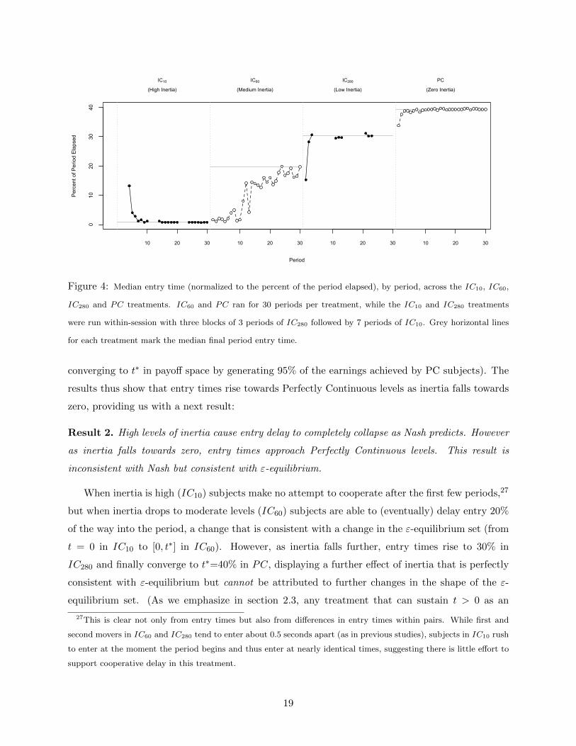
Figure 4 shows the results, plotting period-to-period time series from the IC10 (high inertia),

IC60 (moderate inertia) and IC280 (low inertia) treatments (for reference we also include data from

the zero inertia PC treatment). The results reveal dramatic effects of inertia on continuous time

behavior as inertia drops towards zero. First, the tight entry delays observed in the PC treatment

completely collapses in the high inertia case, generating Perfectly Discrete-like immediate entry as

predicted by Nash after the first few periods. However, when we reduce the severity of inertia, entry

times eventually rise to t = 0.2 at medium inertia and quickly reach t = 0.3 at low inertia (nearly

18

010

2030

40

Period

Per

cent

of P

erio

d E

laps

edIC10

(High Inertia)

IC60

(Medium Inertia)

IC280

(Low Inertia)

PC

(Zero Inertia)

10 20 30 10 20 30 10 20 30 10 20 30

Figure 4: Median entry time (normalized to the percent of the period elapsed), by period, across the IC10, IC60,

IC280 and PC treatments. IC60 and PC ran for 30 periods per treatment, while the IC10 and IC280 treatments

were run within-session with three blocks of 3 periods of IC280 followed by 7 periods of IC10. Grey horizontal lines

for each treatment mark the median final period entry time.

converging to t∗ in payoff space by generating 95% of the earnings achieved by PC subjects). The

results thus show that entry times rise towards Perfectly Continuous levels as inertia falls towards

zero, providing us with a next result:

Result 2. High levels of inertia cause entry delay to completely collapse as Nash predicts. However

as inertia falls towards zero, entry times approach Perfectly Continuous levels. This result is

inconsistent with Nash but consistent with ε-equilibrium.

When inertia is high (IC10) subjects make no attempt to cooperate after the first few periods,27

but when inertia drops to moderate levels (IC60) subjects are able to (eventually) delay entry 20%

of the way into the period, a change that is consistent with a change in the ε-equilibrium set (from

t = 0 in IC10 to [0, t∗] in IC60). However, as inertia falls further, entry times rise to 30% in

IC280 and finally converge to t∗=40% in PC, displaying a further effect of inertia that is perfectly

consistent with ε-equilibrium but cannot be attributed to further changes in the shape of the ε-

equilibrium set. (As we emphasize in section 2.3, any treatment that can sustain t > 0 as an

27This is clear not only from entry times but also from differences in entry times within pairs. While first and

second movers in IC60 and IC280 tend to enter about 0.5 seconds apart (as in previous studies), subjects in IC10 rush

to enter at the moment the period begins and thus enter at nearly identical times, suggesting there is little effort to

support cooperative delay in this treatment.

19

0.0 0.1 0.2 0.3 0.4 0.5

0.5

0.6

0.7

0.8

0.9

1.0

1.1

1.2

Entry Time

Exp

ecte

d Fi

rst M

over

Ear

ning

s

PC (Zero Inertia)IC-280 (Low Inertia)IC-60 (High Inertia)

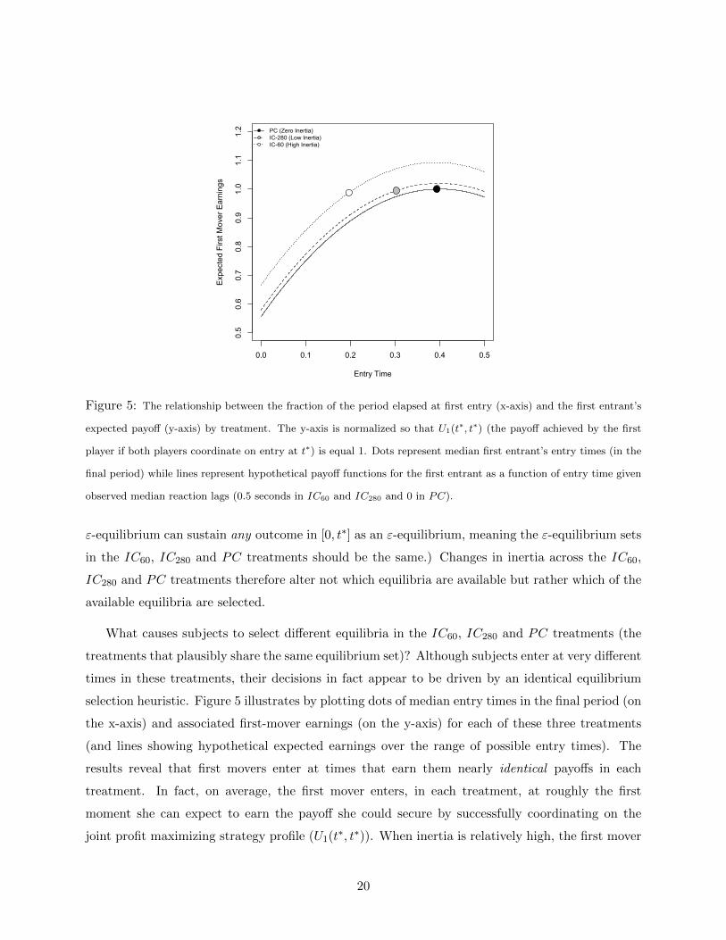
Figure 5: The relationship between the fraction of the period elapsed at first entry (x-axis) and the first entrant’s

expected payoff (y-axis) by treatment. The y-axis is normalized so that U1(t∗, t∗) (the payoff achieved by the first

player if both players coordinate on entry at t∗) is equal 1. Dots represent median first entrant’s entry times (in the

final period) while lines represent hypothetical payoff functions for the first entrant as a function of entry time given

observed median reaction lags (0.5 seconds in IC60 and IC280 and 0 in PC).

ε-equilibrium can sustain any outcome in [0, t∗] as an ε-equilibrium, meaning the ε-equilibrium sets

in the IC60, IC280 and PC treatments should be the same.) Changes in inertia across the IC60,

IC280 and PC treatments therefore alter not which equilibria are available but rather which of the

available equilibria are selected.

What causes subjects to select different equilibria in the IC60, IC280 and PC treatments (the

treatments that plausibly share the same equilibrium set)? Although subjects enter at very different

times in these treatments, their decisions in fact appear to be driven by an identical equilibrium

selection heuristic. Figure 5 illustrates by plotting dots of median entry times in the final period (on

the x-axis) and associated first-mover earnings (on the y-axis) for each of these three treatments

(and lines showing hypothetical expected earnings over the range of possible entry times). The

results reveal that first movers enter at times that earn them nearly identical payoffs in each

treatment. In fact, on average, the first mover enters, in each treatment, at roughly the first

moment she can expect to earn the payoff she could secure by successfully coordinating on the

joint profit maximizing strategy profile (U1(t∗, t∗)). When inertia is relatively high, the first mover

20

can expect to first earn U1(t∗, t∗) by entering at t = 0.2 while when it is low this same payoff

first becomes available later at t = 0.3. When inertia finally reaches zero, subjects can only earn

U1(t∗, t∗) by actually enacting the joint profit maximizing equilibrium by entering at t∗ = 0.4. 28

29 Equilibrium selection in continuous time seems, therefore, to be driven by a focal point in payoff

rather than action space. Because this focal payoff occurs at different entry times for different levels

of inertia, its effect is to push typical behavior further into the ε-equilibrium set as inertia falls to

zero. 30 31

Result 3. When subjects can sustain delayed entry as an equilibrium, they enter at the first time

the U1(t∗, t∗) payoff becomes available. This causes entry to occur closer to t∗ and outcomes to grow

more efficient as inertia drops to zero.

Why do first movers tend to enter when U1(t∗, t∗) first becomes available – why is this payoff

level so focal in our data? We hypothesize that many subjects are willing to deviate from best

response by delaying entry specifically because they hope to achieve the highly salient earnings

level available at the joint profit maximum.32 When this strongly anchored earnings level first

becomes available, much of the motivation for continuing to deviate from best response in order

to improve earnings evaporates and further delay becomes difficult to sustain, causing entry to

occur.33 This heuristic – driven by, but not resulting in, cooperative payoffs – may be important

for selecting equilibria in other dynamic settings as well (e.g. it seems also to explain effects of

payoff matrices on defection times in Inertial Continuous prisoner’s dilemmas)34 and merits further

28To see this note that solving U1(t, t+ δ) = U1(t∗, t∗) yields a t of roughly 0.2, 0.3 and 0.4 in the IC60, IC280 and

PC treatments respectively.29Friedman and Oprea (2012) show a related, complementary result: that Perfectly Discrete time behavior converges

with Inertial Continuous time behavior as the discrete time grid becomes very fine.30Though this focal point yields identical first player payoffs across treatments, it yields higher second player payoffs

as inertia falls. Thus the efficiency of entry tends to increase as inertia approaches zero.31This heuristic seems to organize median behavior not only at the treatment level but also, nearly always, at the

session level. The only exception is a single session of the IC60 treatment where subjects never manage to coordinate

away from the t = 0 equilibrium.32This in fact is close to Radner’s original motivation for ε-equilibrium: agents are willing to deviate from best

response precisely because of the existence of mutual gains from waiting. The existence of further mutual gains

disappears at the first moment that the payoff U1(t∗, t∗) becomes available and this is exactly when subjects tend to

enter in our data.33Note especially that the moment when U1(t∗, t∗) first becomes available is the last moment at which both players

can expect to gain by delaying entry further.34Friedman and Oprea (2012) study 60 second prisoner’s dilemma in Inertial Continuous time under four payoff

matrices and report that subjects tend to use threshold rules, mutually cooperating for most of the period and

mutually defecting towards the end. Our heuristic (given 0.5 reaction lags measured in that data) predict cooperation

collapses at 59.2, 58.8, 58.5 and 57.5 seconds into the period under their easy, mix-A, mix-B and hard payoff matrices,

21

0 10 20 30 40 50

0.0

0.1

0.2

0.3

0.4

0.5

(a)

% of Period Elapsed

Density

PDL-PDPCL-PC

0 10 20 30 40 50

0.0

0.2

0.4

0.6

0.8

1.0

(b)

% of Period ElapsedCDF

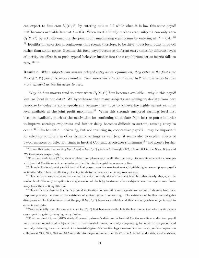
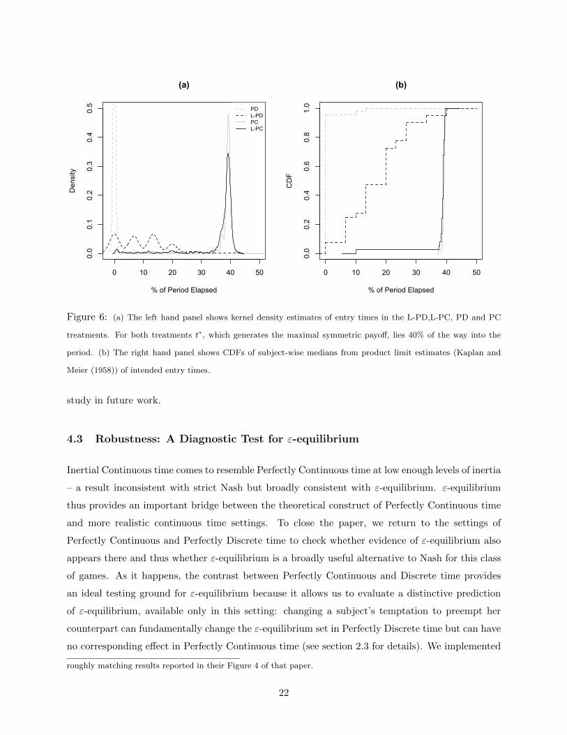
Figure 6: (a) The left hand panel shows kernel density estimates of entry times in the L-PD,L-PC, PD and PC

treatments. For both treatments t∗, which generates the maximal symmetric payoff, lies 40% of the way into the

period. (b) The right hand panel shows CDFs of subject-wise medians from product limit estimates (Kaplan and

Meier (1958)) of intended entry times.

study in future work.

4.3 Robustness: A Diagnostic Test for ε-equilibrium

Inertial Continuous time comes to resemble Perfectly Continuous time at low enough levels of inertia

– a result inconsistent with strict Nash but broadly consistent with ε-equilibrium. ε-equilibrium

thus provides an important bridge between the theoretical construct of Perfectly Continuous time

and more realistic continuous time settings. To close the paper, we return to the settings of

Perfectly Continuous and Perfectly Discrete time to check whether evidence of ε-equilibrium also

appears there and thus whether ε-equilibrium is a broadly useful alternative to Nash for this class

of games. As it happens, the contrast between Perfectly Continuous and Discrete time provides

an ideal testing ground for ε-equilibrium because it allows us to evaluate a distinctive prediction

of ε-equilibrium, available only in this setting: changing a subject’s temptation to preempt her

counterpart can fundamentally change the ε-equilibrium set in Perfectly Discrete time but can have

no corresponding effect in Perfectly Continuous time (see section 2.3 for details). We implemented

roughly matching results reported in their Figure 4 of that paper.

22

our L-PD and L-PC treatments by lowering the ΠF in expressions (1) relative to the PD and

PC treatments. Under the hypothesis of ε-equilibrium, L-PD will expand the ε-equilibrium set,

generating later average entry than PD while L-PC will generate identical behavior to PC. (Of

course, under the hypothesis of Nash the change in parameter should have no effect in either

treatment.)

Figure 6 plots the results from the L-PD and L-PC treatments (and, for reference, results from

the PD and PC treatments in gray). In Perfectly Discrete time the tight immediate-entry pattern

observed under Baseline parameters completely destabilizes with a shift in ΠF . Though a minority

of subjects continue to play the subgame perfect Nash equilibrium, most delay to some degree.

By contrast the change in temptation parameter has no effect on behavior in Perfectly Continuous

Time.35

Result 4. Reducing the temptation to preempt destabilizes the tight mode at zero observed in

Perfectly Discrete time under Baseline parameters but has no corresponding effect in Perfectly

Continuous time. This distinctive pattern is predicted by ε-equilibrium but not Nash.

5 Discussion and Conclusion

Perfectly Continuous and Perfectly Discrete time are both idealizations but they are illuminating

ones, functioning as strategic analogues to vacuums in the physical sciences. Like vacuums, they

are environments in which theoretical forces are cast in particularly high relief and results can

be crisply interpreted in the light of theory. Although Perfectly Discrete time behavior has been

exhaustively studied in thousands of experimental investigations, Perfectly Continuous time has

never been studied before and for a very simple reason: natural frictions in human interaction that

loom especially large in the relatively fast pace setting of a laboratory experiment push strategic

environments meaningfully away from the Perfectly Continuous time setting described in the theory.

Our paper introduces a methodological innovation that eliminates these frictions, allowing us to

observe, for the first time, Perfectly Continuous behavior. By observing and comparing behavior

across these two “pure” environments and by comparing both to more naturalistic protocols in

between we learn some fundamental things about dynamic strategic behavior.

Results from our initial baseline parameters are nearly perfectly organized by benchmarks pro-

35Mann-Whitney tests on session-wise median entry times allows us to reject the hypothesis that L-PD and PD

entry times are equal at the five percent level. An identical test comparing L-PC and PC entry times cannot reject

the hypothesis of equality at any conventional level of significance.

23

posed in the literature. Though our game suffers from multiple (indeed, a continuum of) equilibria

in Perfectly Continuous Time, we observe entry times tightly clustered at the interior joint profit

maximizing entry time under this timing protocol. This decisive equilibrium selection strongly

supports a weak dominance refinement argued for by Simon and Stinchcombe (1989) for Perfectly

Continuous games. By contrast, under the exact same parameters, in Perfectly Discrete Time we

observe almost universal, highly inefficient first-period entry that is perfectly in line with backwards

induction. Thus our baseline results show strong evidence of a large and economically significant

gulf between Perfectly Discrete and Perfectly Continuous time behaviors.

How do results from these artificial settings relate to more realistic strategic interactions? Most

real human decisions are made neither perfectly synchronously (as in Perfectly Discrete time) nor

with instant response (as in Perfectly Continuous time). More realistic are real time, asynchronous

settings in which there is some delay in mutual responses, even if small. Nash equilibrium predicts

that even a tiny amount of such inertia will be sufficient to erase all of the cooperative equilibria

generated by Perfectly Continuous time. However ε-equilibrium suggests that the correspondence

between Inertial Continuous time behavior and the benchmarks of Perfectly Discrete and Perfectly

Continuous time depends crucially on the size of inertia. While very high levels of inertia can cause

ε-equilibrium sets to coincide with Perfectly Discrete behavior (as suggested by Nash), very low

levels of inertia can push the ε-equilibrium set to coincide with the Perfectly Continuous equilibrium

set. We study such settings in our Inertial Continuous time treatments in which subjects interact

(under Baseline parameters) in continuous time but with natural human reaction lags (clocked at

roughly 0.5 seconds in our subjects). By varying the speed of the game clock we are able to alter

the severity of naturally occurring inertia in subjects’ decision making and compare the predictions

of Nash and ε-equilibrium. Our results show that Nash-like collapses to Perfectly Discrete-like

benchmarks do occur in continuous time when inertia is very high. But at low levels of inertia,

subject entry delays approach the efficient levels generated in our Perfectly Continuous treatment.

We close our design by showing that ε-equilibrium also predicts distinctive, asymmetric com-

parative statics in Perfectly Discrete and Perfectly Continuous time that are not predicted by Nash.

Taken together, our data therefore suggests that ε-equilibrium accounts for important ingredients

in behavior that are missing from Nash, at least in our class of games. It bears emphasizing that our

decision to compare Nash to ε-equilibrium was made ex ante and that we designed the experiment

explicitly with this alternative hypothesis in mind. Our reason for focusing the design and analysis

on ε-equilibrium is simply that it plays a central role in motivating results from the prior theoretical

literature (particularly Simon and Stinchcombe (1989) and Bergin and MacLeod (1993)), making

24

it a natural alternative hypothesis to strict Nash for these types of games.36 Our experiment was

not, however, designed to distinguish ε-equilibrium from other alternatives to Nash and we make

no claims that ε-equilibrium is uniquely capable of ex post rationalizing the deviations from Nash

we observe in the data. Indeed common alternatives to Nash contemplated in the literature (i.e.

quantal response equilibrium, level-k models and reputational “gang of four models”) are flexible

enough to rationalize data like ours ex post, under the right parameterizations.37 We conclude that

while ε-equilibrium performed well in anticipating and organizing our data relative to Nash, work

comparing the organizing power of ε-equilibrium to other alternatives to Nash using experiments

designed ex ante for this purpose stands as an important avenue for future research on continuous

time games.

The results from our experiment suggest an appealing framework for understanding the rela-

tionship between the abstractions of Perfectly Discrete and Perfectly Continuous time and real

world behavior. Perfectly Discrete and Perfectly Continuous time predictions can be thought of as

polar outcomes that each approximate realistic (Inertial Continuous time) behavior when inertia

is either very high or very low, respectively. Indeed, we can easily push real time (Inertial) be-

havior close to either Perfectly Discrete or Perfectly Continuous time behavior simply by varying

the severity of inertia. Concretely, these sorts of results suggest that Perfectly Continuous time

benchmarks can, in some cases, be more empirically relevant than Discrete time benchmarks, even

if agents face frictions that should be sufficient to short circuit Perfectly Continuous time equilibria

under standard theory. The rise of thick online global markets, always-accessible mobile technol-

36ε-equilibrium has also been effective at organizing data, ex post, in some recent closely related work. In particular,

Friedman and Oprea (2012) use ε-equilibrium to explain their main results. Bigoni et al. (2015) report data consistent

with ε-equilibrium but, like us, find some treatment variations that change behavior without altering the ε-equilibrium

set. They emphasize the potential additional importance of treatment effects on equilibrium selection – an emphasis

that also seems fitting for our results.37Logit quantal response models for instance cannot rationalize our results with a uniform value of the error

parameter λ but is capable of fitting our data if λ is allowed to vary across treatments. Likewise, level-k models do

a poor job of organizing our data if the level-0 player is assumed to uniformly select an entry time on [0, 1] but do a

quite good job of describing play if we restrict level-0 players to select entry times on [0, t∗]. Finally, “Gang of four”

reputational models (Kreps et al. (1982)) feature many equilibria but, focusing on the equilibrium that has been used

most often for forming hypotheses in the prior experimental literature (a mixed strategy equilibrium, possibly with a

period of pure cooperation before mixing begins, see e.g. Cooper et al. (1996), McKelvey and Palfrey (1992) and Cox

et al. (2015)), our data can be rationalized only if the belief in the prevalence of cooperative types that parameterizes

the model is allowed to vary with treatment (and this belief has to be as large as 50% in some treatments to match

our data). Again, however, we emphasize that the family of reputational models is quite rich, and we can hardly rule

out the possibility that there exist specifications or equilibria that can ex post organize our data in more parsimonious

ways.

25

ogy, friction reducing applications and automated online agents have made strategic interactions

more asynchronous and lags in response less severe. These trends, which seem likely to intensify

in the coming years, have the effect of pushing many interactions closer to the setting of Perfectly

Continuous time. Though these technological changes may never drive inertia entirely to the Per-

fectly Continuous limit of zero, our results suggest that behavior can nonetheless come close to

Perfectly Continuous levels as inertia falls. This deviation from standard theory in turn suggests

that we might expect Perfectly Continuous time predictions to become an increasingly relevant way

of understanding economic behavior relative to the Perfectly Discrete predictions most often used

in economic models.

References

Bergin, James and W. Bentley MacLeod, “Continuous Time Repeated Games,” International

Economic Review, 1993, 34 (1), 21–37.

Berninghaus, S., K.-M. Ehrhart, and M. Ott, “A Network Experiment in Continuous Time:

The Influence of Link Costs,” Experimental Economics, 2006, 9, 237–251.

Bigoni, Maria, Marco Casari, Andrzej Skrzypacz, and Giancarlo Spagnolo, “Time Hori-

zon and Cooperation in Continuous Time,” Econometrica, 2015, 83 (2), 587–616.

Cooper, Russell, Douglas V. Dejong, Robert Forsythe, and Thomas W. Ross, “Coop-

eration without Reputation: Experimental Evidence from Prisoner’s Dilemma Games,” Games

and Economic Behavior, 1996, 12 (2), 187–218.

Cox, Caleb A., Matthew T. Jones, Kevin E. Pflum, and Paul J. Healy, “Revealed Rep-

utations in the Finitely Repeated Prisoner’s Dilemma,” Economic Theory, 2015, Forthcoming.

Deck, C. and N. Nikiforakis, “Perfect and Imperfect Real-Time Monitoring in a Minimum-

Effort Game,” Experimental Economics, 2012, 15, 71–88.

Duffy, John and Jack Ochs, “Equilibrium Selection in Static and Dynamic Entry Games,”

Games and Economic Behavior, 2012, 76, 97–116.

Embrey, Matthew, Guillaume R. Frechette, and Sevgi Yuksel, “Cooperation in the FInitely

Repeated Prisoner’s Dilemma,” December 2014. Mimeo.

Evdokimov, Piotr and David Rahman, “Cooperative Institutions,” August 2014. Mimeo.

26

Friedman, Daniel and Ryan Oprea, “A Continuous Dilemma,” American Economic Review,

2012, 102 (1), 337–363.

Greiner, Ben, Forschung und wissenschaftliches Rechnen, GWDG Bericht,

Kaplan, E.L. and Paul Meier, “Nonparametric Estimation from Incomplete Observations,”

Journal of the American Statistical Association, June 1958, 53 (282), 457–481.

Kreps, David M., Paul Milgrom, John Roberts, and Robert Wilson, “Rational Coop-

eration in the Finitely Repeated Prisoners’ Dilemma,” Journal of Economic Theory, 1982, 27,

245–252.

McKelvey, Richard D. and Thomas R. Palfrey, “An Experimental Study of the Centipede

Game,” 1992, 60 (4), 803–836.

Oprea, Ryan, Gary Charness, and Daniel Friedman, “Continuous Time and Communication

in a Public-Goods Experiment,” Journal of Economic Behaviour and Organization, 2014, 108,

212–223.

, K. Henwood, and Daniel Friedman, “Seperating the Hawks from the Doves: Evidence

from Continuous Time Laboratory Games,” Journal of Economic Theory, 2011, 146, 2206–2225.

Pettit, J., J. Hewitt, and R. Oprea, “Redwood: Software for Graphical Browser-Based Ex-

periments in Discrete and Continuous Time.” Mimeo.

Radner, Roy, “Collusive Behavior in Noncooperative Epsilon-Equilibria of Oligopolies with Long

but Finite Lives,” Journal of Economic Theory, 1980, 22, 136–154.

Simon, Leo K. and Maxwell B. Stinchcombe, “Extensive Form Games in Continuous Time:

Pure Strategies,” Econometrica, 1989, 57 (5), 1171–1214.

27

A Online Theoretical Appendix

In section A.1 we provide proofs for propositions stated in section 2.2 of the main paper. In section

A.2 we prove a set of propositions characterizing ε-equilibrium for our games and provide proofs

for propositions stated in section 2.3 of the main paper.

A.1 Nash Equilibrium

In subsection A.1.1 we prove proposition 1, which relies exclusively on standard theoretical tools.

In subsection A.1.2 we provide more details on the theoretical schema of Simon and Stinchcombe

(1989) and provide a self contained heuristic proof of proposition 2 following the intuition of Simon

and Stinchcombe (1989). We close the subsection by providing a full proof of proposition 2 that

draws directly on theoretical machinery developed in Simon and Stinchcombe (1989). Because this

machinery is substantial, this full proof is not self contained and relies on definitions and lemmas

developed in Simon and Stinchcombe (1989).

In subsection A.1.3 we provide some details on the theoretical apparatus of Bergin and MacLeod

(1993), an alternative way of modeling continuous time games, and specialize it to our setting. We

then re-prove proposition 2 using this method. Again, because the required tools are substantial,

this proof is not self contained but draws on definitions and results from Bergin and MacLeod

(1993). Finally, we use ideas from Bergin and MacLeod (1993) to prove proposition 3.

A.1.1 Proof of Proposition 1

Proof of Proposition 1. We prove by contradiction. First, consider the case of pure strategies:

Suppose that there is an equilibrium where player i enters at a weakly later grid point than player

j, and that this is not the first grid point. Player i has a profitable deviation, which is to enter

one grid point before player j or at the first grid point if there are no grid points before player j’s

entry time. Contradiction.

The modification to allow for mixed strategies is straightforward. Call the last grid point that

player i places positive weight on ki. Suppose that there is an equilibrium with ki ≥ kj and ki 6= 0

(where we are labeling t = 0 as the zeroth grid point). Player i can improve their payoff by moving

weight from entry at ki to entry at the grid point identified by max{kj − 1, 0}.

28

A.1.2 Simon and Stinchcombe (1989)

In this section, following Simon and Stinchcombe (1989), we model our game by considering a set

of strategies that are unambiguously defined in the limit of a discrete time grid as the grid becomes

infinitely fine. Together, the two player game generated by the utility function in equation 1, the

histories Ht and strategies si given below define what we call the Perfectly Continuous time game.38

We begin by defining a history, and use the history to define a set of strategies.

In our timing game, a history consists of two pieces of information: the current time, and a

record of players that have already entered the market. Therefore, a history at time t, Ht, is an

object in [[0, t] ∪ {1}]2, where the first element denotes the entry time for firm i, and the second

element the entry time for firm j, with 1 indicating that a firm has not yet entered. For example,

a history at time t = 0.5 can be written H0.5 = {0.4, 1}0.5, indicating that the first firm entered at

time t = 0.4, the second firm is yet to enter, and the subscript denotes the current time.

Given this definition of histories, a strategy is a mapping si : Ht 7→ {0, 1}, where 1 indicates an

action of “enter” at that history. We fix si({t′, ·}t) = 1 for all t′ < t (after a firm has entered they

cannot leave the market again), require that si is a piecewise continuous function, and also require

that if si({1, t′}t) = 1 then si({1, t̂}t) = 1 for all t̂ ≤ t′ (if, at time t, I wish to enter in response to

an opponent who entered at time t′ then I must also enter in response to any opponent that entered

prior to t′). Notice that these strategies satisfy assumptions F1 - F3 of Simon and Stinchcombe

(1989).39

Most of the technical complications that arise from modeling games in continuous time are

related to the “well-ordering paradox” that, in continuous time, the notions of “the next moment”

or “the previous moment” have no meaning. As Simon and Stinchcombe (1989) point out this

means that sensible sounding strategies such as “I play left at time zero; at every subsequent

time, play the action I played last period” are not well defined. The approach that Simon and

Stinchcombe take is to restrict attention to strategies that are uniquely defined as the limit point

for any discrete time grid as the grid becomes arbitrarily fine; their conditions F1-F3 are designed

to generate such strategies.

38The strategies also implicitly define the action sets and the allowable order of moves, and the game is of complete

and perfect information.39The conditions require a bounded number of changes in action for each player, piecewise continuity with respect

to time and strong right continuity with respect to histories. The first two are obviously satisfied here, and the

requirement that si({1, t′}t) = 1 then si({1, t̂}t) = 1 for all t̂ ≤ t ensures strong right continuity with respect to

histories.

29

We present two proofs of proposition 2 in this section that follow this modeling approach. The

first proof, which we call the “heuristic proof” does not directly address many of the complexities

associated with continuous time, other than to restrict the strategy set to the strategies defined

above. The question of whether this restriction is appropriate is not undertaken here. For this

reason we also provide an alternative proof, resting almost entirely on results in Simon and Stinch-

combe (1989), which demonstrates that our equilibria are sound. We also provide a heuristic proof

of remark 1.

Heuristic proof of proposition 2. Consider, the strategies:

st′i (Ht) =

0 if Ht = {1, 1}t with 0 ≤ t < t′ ≤ t∗

1 otherwise(2)

Each of these strategies generates simultaneous entry at t′. To aid intuition, we focus on these

strategies precisely because they are strategies such that there is no delay in responding to an

opponent’s entry in any history. Such a delay is (weakly) payoff decreasing, and certainly cannot

be observed in an equilibrium. More formally, this implies ruling out all strategies si(Ht) = 0 where

Ht = {1, t′} for t′ < t.

We claim that the strategies given in equation 2 form a set of (symmetric) equilibria. That is,

the pair of strategies (st′i (Ht), s

t′j (Ht)) are an equilibrium of our Perfectly Continuous time game.

To see that this is true, consider two cases.

In the first case, consider a strategy that deviates from st′i (Ht) by replacing st

′i = 1 with s′t

′i = 0

for some set of histories. Given our restriction that a firm cannot re-enter after it has exited, this

can only occur for histories in which the firm has not yet entered. This implies that these must be

histories in which either our opponent has entered, or no one has entered. Histories in which no

one has entered at times after t′ are off the equilibrium path, so the change in strategy profile has

no effect on payoffs. Histories in which the opponent has entered will either be off the equilibrium

path, or on a path for which U(st′i , s

t′j ) > U(s′t

′i , s

t′j ) (this is because the payoff for the second

entrant is a decreasing function of their entry time).

In the second case, consider a strategy that deviates from st′i (Ht) by replacing st

′i = 0 with

s′t′i = 1 for some set of histories. It must be the case that at least one of these histories is on the

equilibrium path: s′ will cause the firm to enter before t′. Given the equilibrium strategies this

deviation will generate an instantaneous reply from the firm’s opponent. We shall now observe joint

entry at some time prior to t′. Given that the payoff to joint entry is increasing on the interval

30

[0, t∗], such a deviation reduces the firms payoff.

Heuristic proof of remark 1. We proceed somewhat unusually and consider the second round of

iterated elimination of weakly dominated strategies first.

Consider the strategies used to build the equilibrium in the heuristic proof of proposition 2.

Given that we restrict attention to only these strategies, each of the strategies of the type given in

equation 2 is weakly dominated by the strategy

si(Ht) =

0 if Ht = {1, 1} with 0 ≤ t < t∗

1 otherwise(3)

which generates joint equilibrium entry at t∗.

We now show that any strategy not in equation 2 is weakly dominated by a strategy that is in

equation 2.

Consider the class of strategies that has si({1, 1}t) = 0 for all t < t′ and si({1, 1}t′) = 1. Each

strategy in this class is weakly dominated by st′i as defined in equation 2.40 If their opponent is

yet to enter by t = t′ then all strategies in the class provide the same utility. The only way that

strategies in the same class can differ is in how they respond to entry from their opponent: because

st′i responds instantly in all cases, each other strategy in the class must have a delay in response

for at least some opponent entry time. Given that payoffs are decreasing in the entry time of the

second firm, the dominance relation is established.

All strategies must fall into one of the above classes.

The strategy in equation 3 is therefore the unique strategy that survives iterated elimination of

weakly dominated strategies.

We conclude this section with a more formal (but less self contained) proof of proposition 2,

drawing more directly on definitions and results from Simon and Stinchcombe (1989).

Formal proof of Proposition 2. The proof consists entirely of demonstrating that Theorem 3 of

40Or, if t′ > t∗ in violation of 2, then the strategy is weakly dominated by st∗i .

31

Simon and Stinchcombe (1989) is applicable to our environment. We begin by stating this theorem.

The definitions of all relevant notation can be found in Simon and Stinchcombe (1989).

Theorem 1 (Theorem 3 from Simon and Stinchcombe (1989).). Consider a continuous-time game

with a dH-continuous valuation function. Let f be a continuous-time strategy profile satisfying F1-

F3. Suppose that there exists a sequence of δn-fine grids, (Rn), where δn →n 0 and a sequence (gn,

εn) such that εn →n 0 and for each n, gn is an εn-SGP equilibrium for the game played on Rn.

Further suppose that gn is defined by further restricting f|Rn to the R-admissible decision nodes.

Then f is an SGP equilibrium for the continuous time game.

We proceed in 5 steps:

1. The game has a dH -continuous valuation function because all games with integrable flow

payoff functions, such as ours, have a dH -continuous valuation function.

2. Label the strategy profile that induces entry at time t in equation 2 as f(t). f(t) satisfies

Simon and Stinchcombe (1989)’s conditions F1-F3.

3. Take the sequence of grids to be grids with G = n uniformly spaced points.

4. Define g(t)n to be the strategy profile where each agent plays “enter” at all grid points that

occur (weakly) after t. At all grid points (strictly) before t, each agent plays “wait” if both

agents have played “wait” at all previous grid points and otherwise they play “enter”. This

strategy is the restriction f|Rn to the R-admissible decision nodes.

5. It follows immediately from the proof of proposition 6 that g(t)n forms an ε(t)n-equilibrium

where ε(t)n is defined by replacing the inequality in equation 5 with equality. Furthermore,

ε(t)n → 0 as G = n→∞.

We therefore conclude that f(t) is an equilibrium of the continuous time game. We finish by

noting that the strategy f(t) induces an outcome where both agents enter at time t, and that

the definition of f(t) allows 0 < t ≤ t∗. Joint entry at t = 0 is obviously also supported by an

equilibrium (if your opponent enters at t = 0 then your best response is also to enter at t = 0).

Therefore, we can support entry at any time t ∈ [0, t∗] as an equilibrium in the continuous time

game.

32

A.1.3 Bergin and MacLeod (1993)

Bergin and MacLeod (1993) take an alternative approach to modeling continuous time games

by introducing a general notion of inertia and modeling continuous time as the limit as inertia

disappears.41 In this subsection, we first formally define a narrower notion of reaction-lag-based

inertia appropriate for the setting of our experiment. We then prove proposition 3 which claims that

short of the condition limit (i.e. when inertia is greater than zero) firms must enter immediately (at

t = 0) in equilibrium. Finally, we provide an alternative proof of proposition 2 using proposition

3 and Bergin and MacLeod (1993)’s Theorem 3. By doing so, we show that in our game the two

approaches to modeling Perfectly Continuous time – e.g. as the limit of Perfectly Discrete time ala

Simon and Stinchcombe (1989) or as the limit of Inertial Continuous time ala Bergin and MacLeod

(1993) – make identical predictions.42

We introduce a simplified version of Bergin and MacLeod (1993)’s definition of inertia that is

appropriate for our game, capturing the key idea of inertia as a reaction lag.43

Definition 1 (Inertia). Fix a time t̂ ∈ [0, t∗]. Suppose that si({1, 1}t) = 0 for all t < t̂ and that

si({1, 1}t̂) = 1. A strategy satisfies inertia if there exists a δ > 0 such that si({1, t′}t) = 0 for all

t, t′ such that t′ ≤ t < min{t̂, t′ + δ}.

Our inertia condition prevents firms from responding immediately to the entry decisions of their

opponents - responses are delayed by at least δ > 0 of the game.44 We can think of t̂ as a firm’s

planned entry time – if their opponent has not entered yet, then the firm plans to enter at t̂. The

inertial requirement then states that the firm cannot enter within δ of their opponent’s entry time,

unless they are entering at their planned entry time.

We define Inertial Continuous time simply as Perfectly Continuous time restricted to strategies

that satisfy the inertia condition of definition 1 and can use this to provide a proof of proposition

41A key technical innovation of Bergin and MacLeod (1993) is that it allows one to model continuous time in

infinitely repeated games. Infinitely repeated games violate the Simon and Stinchcombe (1989) assumption that an

agent will change their behaviour a finite number of times.42We conjecture that this is also true more generally, whenever the relevant conditions of both Bergin and MacLeod

(1993) and Simon and Stinchcombe (1989) are satisfied.43Bergin and MacLeod (1993) assume that the action space is constant across time, violating a condition in our

experiment: we do not allow firms to exit the market once they have entered (i.e. once a firm has exited their action

space shrinks from two actions to only one action). This technical problem can be neatly resolved by imposing an

artificially large amount of inertia to all histories in which the firm has already entered.44Recall that we define δ ≡ δ0

T, where δ0 is a subject’s natural reaction lag in real time and T is the game length

in real time.

33

3.

Proof of proposition 3. The pure strategy case provides the intuition for the full proof, so we first

prove that there are no pure strategy equilibria with delayed entry.

We proceed by contradiction. Suppose that there is a pure strategy equilibrium where the

earliest entry is not at time 0. Without loss of generality assume that firm i enters weakly before

firm j at time t > 0. It is easy to verify that firm j has a profitable deviation: entering at a point

that is δ before t (or at 0 if t < δ). This contradicts the assumption that the strategies form an

equilibrium.

To deal with mixed strategies, the proof by contradiction needs only minimal changes. Write

tj > 0 and ti for the latest entry time used by firms j and i in a mixed strategy equilibrium for

histories where their opponent has yet to enter. We proceed by demonstrating that there is a

strategy in the support of player j’s mix that is not optimal.

Suppose that tj ≥ ti. Consider the history where we arrive at time max{ti − δ, 0} and neither

firm has entered yet. Clearly firm j’s strategy is not optimal: given firm i’s strategy, and the fact

that we reach the current subgame with positive probability, firm j should enter immediately with

certainty. This contradicts the assumption that the strategies form an equilibrium.

The logic behind the proofs of propositions 1 and 3 does not apply to proposition 2. The reason

is that in continuous time a firm can respond instantaneously to its opponent’s entry. The logic of

the proof by contradiction thus does not hold: firm j’s best response is no longer to preempt firm

i, but to enter simultaneously with firm i. We conclude the section with an alternative proof of

proposition 2.

Alternative proof of Proposition 2 using Bergin and MacLeod (1993). The proof consists entirely

of demonstrating that Theorem 3 of Bergin and MacLeod (1993) is applicable to our environment.

There are some technical hurdles to be surmounted as Bergin and MacLeod (1993) define strate-

gies as being mappings from outcomes to actions, rather than the more standard mappings from

histories to actions. Fortunately, in our game, there is a straightforward mapping from histories to

outcomes that simplifies matters greatly.

We first state Bergin and MacLeod’s Theorem 3:

Theorem 2 (Theorem 3 from Bergin and MacLeod (1993)). A strategy x ∈ S∗ is a subgame perfect

equilibrium if and only for any Cauchy sequence, {xn} converging to x, there is a sequence εn → 0,

34

such that xn is an εn-subgame perfect equilibrium.

To start, we note that although the theorem implies that all convergent Cauchy sequences need

to form a convergent sequence of ε-equilibrium it is clear from Bergin and MacLeod’s proof that

it is sufficient to find a single satisfactory sequence. Once a single sequence is found, part (b) of

their proof implies that x is an equilibrium and then part (a) of their proof implies that all other

convergent sequences must also have associated convergent ε paths.

We note again that Bergin and MacLeod (1993) use a special domain for their strategies. The

domain of x is the object (A, T ) where A = {ti, tj} is a set of outcomes (one for each player) and

T = [0, 1] is the set of feasible entry times. Clearly, we can translate each of our strategies into the

Bergin and MacLeod (1993) formulation. For example, the strategy that induces player i to enter

at the earlier of time τ and immediately after their opponent enters could be written as:

x1((·, tj), t) =

0 if t < τ and t < tj

1 otherwise(4)

The set of strategies that satisfy our inertia condition (definition 1) maps into a subset of Bergin

and MacLeod’s set of strategies S. If we add the set of strategies that are formed in the limit as

δ → 0, then we have a set of strategies that are a subset of Bergin and MacLeod’s set of strategies

S∗.45

Now, for each time τ ∈ [0, t∗], let x(τ)n be a sequence of strategies for both players that satisfy

definition 1 with τ = t̂ and δ = δn such that δn → 0. Then x(τ)n Cauchy converges to the strategy

given in equation 4. Furthermore, from the proof of proposition 7, for each x(τ)n we can identify

an εn, which is found by replacing the inequality in equation 8 with an equality, such that the

strategies form an εn-equilibrium. Clearly, the sequence εn → 0 as δn → 0.

Therefore, we conclude that the strategy x(τ), which generates joint entry at t = τ , forms an

equilibrium of the continuous time game. Given that this is true for all τ ∈ [0, t∗], we can sustain

all such entry times in equilibrium.

45Note that the strategy presented in equation 4 is in S∗ but not in S because it does not satisfy the inertia

condition.

35

A.2 ε-equilibrium

In subsection A.2.1 we prove three propositions that completely characterize the ε-equilibrium

sets for each of our timing protocols. In appendix A.2.2 we use these characterizations to prove

comparative static propositions stated in section 2.3 that form the basis of alternative hypotheses

for the experiment.

Following Radner (1980) we assume that players are willing to tolerate a payoff deviation from

best response of size ε and treat their counterparts as having the same tolerance. We can then

form a set of propositions that provide alternative predictions to Nash as a function of ε for each

of our three main protocols.

A.2.1 Characterization of ε-equilibrium Sets

Again, we begin by considering Perfectly Discrete Time. Recall that for a game with grid size G,

dates begin at t ={

0, 1G ,

2G , ..., 1

}(a total of G + 1 dates). For notational simplicity, assume that

the grid is such that t∗ = 1 − ΠD4c lies exactly on some grid point (this assumption simplifies the

following expressions and is imposed in the parameterization of our experiment), and label this

gridpoint kG .

Proposition 6. Suppose that all agents enter at or before t∗.46 In a Perfectly Discrete time game

with G + 1 periods, t∗ = kG and tolerance ε the set of entry times that can be sustained in a pure

strategy sub-game perfect ε-equilibrium is given by{

0, 1G , ...,

κG

}where κ is the largest integer that

satisfies 0 ≤ κ ≤ k and

1

G

[3ΠF

2− c(2 +

1

G)

]+

κ

G2

[2c− ΠF

2

]≤ ε. (5)

If no non-negative integer satisfies equation 5 then κ = 0 (i.e. the unique equilibrium is immediate

entry).

Proof of proposition 6. We begin with two assumptions. Firstly, we assume that all firms enter at

or before t∗. Secondly, when one firm enters the other firm shall enter as soon as possible afterwards

(in the next sub period). We shall demonstrate at the end of the proof that the second assumption

can be disposed of, but imposing it simplifies the proof.

46If the ε-equilibrium set includes t∗, it is possible for entry times after t∗ to also be supported as ε-equilibria.

Such entry times never arise in the data and violate the conceptual spirit of ε-equilibrium outlined by Radner (see

Footnote 12) and we assume them away purely to simplify the discussion and notation.

36

We proceed by backwards induction. Suppose that firms arrive at period k−1 and neither firm

has entered yet. We are interested in determining whether cooperation can be sustained for one

more period. If it can, then the payoff to each firm will be U( kG ,kG). If, however, a firm defects and

enters immediately then they will earn U(k−1G , kG).

After some algebra, we see that U(k−1G , kG)− U( kG ,

kG) = 1

G

[3ΠF

2 − c(2 + 1G)]

+ kG2

[2c− ΠF

2

].

Therefore, we conclude that if neither firm has entered when firms arrive at period k − 1, then

joint entry at period k can be sustained as an ε-equilibrium if

ε ≥ U(k − 1

G,k

G)− U(

k

G,k

G). (6)

Now, rollback to period k − 2. Suppose that firms arrive at period k − 2 and neither firm has

entered yet. Can cooperation be sustained for one more period? There are two cases.

In the first case equation 6 holds, so that if both firms wait at period k − 2 then there is

an equilibrium continuation where each firm earns U( kG ,kG). If, however, a firm enters at period

k − 2 they will earn U(k−2G , k−1

G ). Waiting can therefore be sustained as an ε-equilibrium if ε ≥

U(k−2G , k−1

G ) − U( kG ,kG). This inequality must hold whenever equation 6 holds because the utility

function is increasing in (joint delay of) entry times. We therefore conclude that if both firms may

wait in an ε-equilibrium at period k−1 then they may also wait in an ε-equilibrium at period k−2

(and the same logic implies this must be true for any earlier period as well).

In the second case equation 6 does not hold. Therefore, if both firms wait at period k − 2

they must both enter at period k − 1 and the continuation payoff is U(k−1G , k−1

G ) for both firms.

Defecting to immediate entry will earn U(k−2G , k−1

G ).

After some algebra, we see that U(k−2G , k−1

G )−U(k−1G , k−1

G ) = 1G

[3ΠF

2 − c(2 + 1G)]+k−1

G2

[2c− ΠF

2

]<

U(k−1G , kG)− U( kG ,

kG).

Therefore, we conclude that if neither firm has entered when firms arrive at period k − 2, then

joint entry at period k − 1 can be sustained as an ε-equilibrium if ε ≥ U(k−2G , k−1

G )− U(k−1G , k−1

G ).

Notice that the ε cutoff at period k − 2 is less than the cutoff at k − 1. Therefore, there are some

ε values where co-operation can be sustained at period k − 2, but not at period k − 1.

The proof continues by induction, rolling back one period at a time and noting that U(k−n−1G , k−nG )−

U(k−nG , k−nG ) is decreasing in n, and substituting n = κ delivers the equation in the proposition.

We still need to demonstrate that relaxing our initial assumption that entry by one firm would be

immediately followed by entry from the other will not change the equilibrium set found above. There

37

are two concerns: firstly, that allowing lengthier delays might destroy some equilibria described

above and, secondly, that allowing lengthier delay might create new equilibria.47

No equilibria can be destroyed. Take an equilibrium found above, and allow an agent to uni-

laterally deviate to a strategy that involves lengthy delays after their opponent’s entry (in at least

some subgames). This deviation must weakly decrease the agent’s payoff, so it is not a profitable

deviation and the original equilibrium survives.

New equilibria can be created, but none of these equilibria will involve an initial entry time

that is later than the set of entry times described in the proposition. We demonstrate this with a

proof by contradiction. For a given ε, define κ as given by equation 5. Now, suppose that there is

an equilibrium with entry at the pair of nodes (κ+jG , κ+j+i

G ) with j ≥ 1 and i ≥ 2. Then, from the

definition of ε-equilibrium it must be the case that U(κ+j−1G , κ+j

G )− U(κ+j+iG , κ+j

G ) ≤ ε (otherwise

the second entrant would have a profitable deviation).

Now, it is also true that U(κ+j−1G , κ+j

G ) − U(κ+j+iG , κ+j

G ) > U(κ+j−1G , κ+j

G ) − U(κ+j+1G , κ+j

G ) ≥

U( κG ,κ+1G )− U(κ+2

G , κ+1G ) > U( κG ,

κ+1G )− U(κ+1

G , κ+1G ) > ε.

The second inequality is demonstrated by writing out U(k−1G , kG)−U(k+1

G , kG), collecting terms

and noting that the coefficient on k is 8c−(ΠF+ΠS)2G2 > 0 (intuitively, this is demonstrating that the

payoff difference between preempting rather than being preempted is increasing in time). The final

equality follows from the definition of κ. This establishes the contradiction.

We now characterize the ε-equilibrium set for Inertial Continuous time.

Proposition 7. Assume that both firms enter at some time t ≤ t∗.48 In an inertial continuous

time game with inertial delay δ, and tolerance ε, all entry times t ∈ (0, τ̄ ] can be sustained in a

subgame perfect ε-equilibrium where τ̄ is the solution to:

arg maxτ∈(0,t∗]

τ (7)

s.t. δ

[(1− τ

2+ 1

)ΠF − c(2− 2τ + δ)

]≤ ε. (8)

47Intuitively, one way to view this is to think of longer delays as being analogous to a game where the grid becomes

coarser after one player has entered. This increases returns to defection and therefore shrinks the equilibrium set.48See Footnote 46.

38

If no such τ exists then the unique equilibrium entry time is t = 0.

Proof of proposition 7. The proof technique is the same as for proposition 6. Again, we begin

by assuming immediate response (or as soon as possible given the reaction lag) to an entry, and

establish that it can be discarded ex-post.

Consider a strategy such that each firm enters at t = τ if their opponent has yet to enter at

τ , and they enter as soon as possible if their opponent enters before τ . A best response to such a

strategy is to to enter at τ − δ, and enter as soon as possible if their opponent enters before τ − δ.

Notice that entering in range (τ − δ, τ) is not a best response because of the assumption implicit

in definition 1 which tells us that the opponent could still enter at τ in this case.

The payoff from waiting both firms waiting until τ is given by U(τ, τ), and the best response

strategy of entering at τ − δ earns a payoff of U(τ − δ, τ).

Observe that U(τ − δ, τ)−U(τ, τ) = δ[(

1−τ2 + 1

)ΠF − c(2− 2τ + δ)

], and that this expression

is increasing in τ .

We therefore conclude that the strategy considered above can be sustained as an ε-equilibrium

if ε ≥ δ[(

1−τ2 + 1

)ΠF − c(2− 2τ + δ)

].

This establishes the proposition.

As dealt with in the proof of proposition 6, it is possible to discard the assumption of immediate

response. Suppose that there is an ε-equilibrium where there is a delay δ̂ > δ between entry times

and that the first entry time occurs at t > τ̄ where τ̄ is the largest solution to equation 8. The

payoff for the second mover is then given by U(t + δ̂, t). The assumption that this constitutes

a subgame perfect ε-equilibrium implies that U(t − δ, t) − U(t + δ̂, t) ≤ ε. But, we also have

U(t − δ, t) − U(t + δ̂, t) > U(t − δ, t) − U(t + δ, t) > U(τ̄ − δ, τ̄) − U(τ̄ + δ, τ̄) > U(τ̄ − δ, τ̄) −

U(τ̄ + δ, τ̄) > U(τ̄ − δ, τ̄)−U(τ̄ , τ̄) = ε. Note that the second inequality follows from the derivatived(U(t−δ,t)−U(t+δ,t))

dt = δ2 [8c− (ΠF + ΠS)] > 0, and that the final equality follows from the definition

of τ̄ . We have reached a contradiction, and reject the existence of such equilibria.

Finally, we note that the central motivation for ε-equilibrium – that agents are willing to tolerate

small deviations from best response in order to achieve high, cooperative payouts – loses its bite

in Perfectly Continuous time where agents can achieve these same payouts without deviating from

best response at all. For completeness we state this as a final proposition.

39

Proposition 8. Assume that all agents enter at or before t∗.49 In Perfectly Continuous Time, the

set of Nash equilibrium entry times and the set of ε-equilibrium entry times are identical for any ε:

any entry time t ∈ [0, t∗] can be supported in either case.

Proof of proposition 8. The Nash equilibrium set is given by proposition 2. All Nash equilibria are

ε-equilibria, so all entry times t ∈ [0, t∗] can also be supported in an ε-equilibrium. The proposition

rules out entry times after t∗ by assumption, so the two equilibrium sets are identical over the

allowable range of entry times.50

A.2.2 ε-equilibrium: Proofs of Propositions Stated in Section 2.3

In this subsection we use the preceding characterizations to prove propositions from section 2.3.

Proof of proposition 4. Proposition 4 is an application of proposition 7.

Substituting t∗ into equation 8, we see that t∗ is an equilibrium for any ε > 0 when δ satisfies:

δ

[(1− t∗

2+ 1

)ΠF − c(2− 2t∗ + δ)

]≤ ε. (9)

Equation 9 bounds a quadratic equation in δ with negative leading coefficient, so that any

δ less than the smaller root will satisfy our requirements. Denote this root by δ̃ and write b =

(1−t∗2 + 1)ΠF − c(2− 2t∗) for convenience. The ever-handy quadratic formula delivers:

δ̃ =b

2c−√

b2

4c2− ε

c

Noting that δ̃ is always positive whenever ε > 0 completes the proof of the first part of the

proposition.

For the second part of the proposition, note that because inertia cannot exceed the total game

length δ ≤ 1. Substituting τ = 0 into equation 8 we find that there will exist a ε-equilibrium with

at least some delay if there exists a δ ∈ (0, 1] that is a solution to:

49See Footnote 46.50Again, in Perfectly Continuous time, it is possible to support entry times after t∗ in an ε-equilibrium. All such

equilibria would, however, be ruled out by applying Simon and Stinchcombe’s 1989 iterated elimination of weakly

dominated strategies argument.

40

δ

[3

2ΠF − c(2 + δ)

]= ε.

The left hand side of this equation is a quadratic in δ with negative leading coefficient which

reaches a maximum on the interval [0, 1] at δ = 1 if ΠF >8c3 and at δ = 3ΠF

4c − 1 if ΠF ≤ 8c3 . The

value of the left hand side at these points are the values of ε̂ as given in the proposition.

The upper bound in the proposition, ε̂, is a natural consequence of the “thick” indifference

curves that are associated with large values of ε. For any game with bounded payoffs there will

exist a ε large enough that an agent is indifferent between all outcomes, and all outcomes may

therefore be sustained in a ε-equilibrium. The restriction that ε ≤ ε̂ can therefore be viewed as a

non-triviality requirement.

Proof of proposition 5. Proposition 5 is a straightforward application of propositions 6 and 8.

From equation 5, the coefficient on ΠF is 12G

(3− κ

G

)> 0. Therefore, decreasing ΠF reduces

the LHS of equation 5. Therefore, as ΠF decreases the largest value of κ that satisfies equation 5

weakly increases.

From proposition 8, the ε-equilibrium set in perfectly continuous time is independent of ΠF .

41

B Online Instructions to Subjects

Instructions

You are about to participate in an experiment in the economics of decision-making. If you follow

these instructions carefully and make good decisions, you can earn a CONSIDERABLE AMOUNT

OF MONEY, which will be PAID TO YOU IN CASH at the end of the experiment.

Your computer screen will display useful information. Remember that the information on

your computer screen is PRIVATE. To insure best results for yourself and accurate data for the

experimenters, please DO NOT COMMUNICATE with the other participants at any point during

the experiment. If you have any questions, or need assistance of any kind, raise your hand and the

experimenter will come and help you.

In the experiment you will make decisions over several periods. At the end of the last period

you will be paid, in cash, the sum of your earnings over all periods.

The Basic Idea.

In each of several periods, you will be randomly matched with another participant for 60

seconds and you will each decide when to Enter the market. If you both enter at the same time,

you will both earn the same amount, which will depend on the time at which you both entered.

If one player enters earlier than the other, she will earn more money while her counterpart will

earn less. The longer the second player waits to enter after the first player enters, the greater the

difference in their earnings.

Screen Information.

A vertical dashed line marks the passage of time, moving from left to right over the course of the

period until both players have chosen to Enter the Market. A dot moving left to right labeled

‘Me’ and another labeled ‘Other’ shows payment information for each player, although before either

player has entered the market the two dots will be precisely on top of each other. The dots show

the amount of money each subject will earn if both players have entered now If nobody has entered

yet the dots (which are on top each other) show what will happen if both enter now. If one player

has entered already the dots (which are now separated) will show the amount each player will earn

if the second player enters the market now.

42

Figure 7: Nobody has entered.Figure 8: One player has decided to enter and the clock

has frozen.

You can choose to Enter the market at any time by pressing the space bar. The time of entry

will be shown on the screen as a dashed vertical line.

The screen gives you information on your potential earnings under three possible scenarios:

If you both enter in the same sub-period

If you and your counterpart enter at the same time, you will earn exactly the same amount as

your counterpart. The black line that looks like a hill shows exactly what you and your counterpart

would both earn if you both entered in each moment of the period.

Notice that your joint earnings depend on when you both choose to enter in. For example, if

you and your counterpart both entered at time 0, you would both earn 20 points. However, if you

both entered at time 24, you would both earn approximately 36 points.

If you enter first

If your counterpart enters later than you, she will earn less and you will earn more than if she

had entered at the same time you did. At every moment the screen tells you what would happen

if you entered now, and your counterpart entered at a later time than you:

43

• The green line shows you what you would earn if you entered now and your counterpart

entered in each of the remaining moments in the period.

• The red line shows you what your counterpart would earn if you entered now and she entered

in each of the remaining moments in the period.

Notice that the longer your counterpart waits to enter after you, the less she earns. For instance

in the example in Figure 1, if you entered now and your counterpart entered 5 seconds later, you

would earn approximately 38 points (the amount on the green line 5 seconds later) and your

counterpart would earn approximately 20 points (the amount on the red line 5 seconds later). If,

instead, your counterpart waited 10 seconds to enter, you would earn approximately 50 points and

your counterpart approximately 18 points.

Note that these lines will change as you move along: the green line will always be above the

current point on the black hill and the red line will always be below, reflecting the fact that you

earn more (and your counterpart less) than if your counterpart entered when you did.

If you enter second

If you enter at a later time than your counterpart, you will earn less and your counterpart more

than if you had moved at the same time as your counterpart. Importantly, these graphs and payoffs

are symmetric: your counterpart sees the same screen (at least prior to anyone entering) and faces

the same payoff consequences as you do. Thus it is also true that:

• The green line shows you what your counterpart would earn if (s)he entered now and you

entered later at a future time.

• The red line shows you what you would earn if your counterpart entered now and you entered

at a later time.

For instance in the example in Figure 1, if your counterpart entered now and you entered in

5 seconds, your counterpart would earn approximately 38 points (the amount on the green line 5

seconds to the right) and you would earn approximately 20 points (the amount on the red line 5

seconds to the right). If, instead, you waited 10 seconds to enter, you would earn approximately

18 points and your counterpart approximately 50 points.

44

Time Freeze

After a player first enters, the game will freeze for 5 seconds. During these 5 seconds the

player’s counterpart can choose whether to enter too by pressing the spacebar. If (s)he does, the

software will treat both entry decisions as occurring at the same time and both players will

earn the exact same amount (the amount shown on the black line at the moment of entry). If she

does not choose to enter during the time freeze, the clock will resume and her earnings will drop,

following the red line. The time freeze is demonstrated in Figure 2.

After Entry Occurs

If one player enters before the other, you will see a dotted green line mark the time of first entry

and you will see the dots separate, one following the green line and the other red line. A label next

to each dot will tell you which corresponds to you (labeled “Me”) and which to your counterpart

(labeled “Other”). A message at the top of the screen will also remind you whether you were the

first to enter (in green) or the second (in red). If you were not the first to enter, the timing of your

entry decision will now determine both of your earnings. Figure 3 shows an example.

After both players enter, horizontal lines will appear showing your earnings. At the end of these

lines (on the right side of the screen) you will see your and your counterparts’ exact earnings (if you

both entered at the same time, you will both earn the same amount). Figure 10 shows an example

in which one player has entered at time 10 and the other later at time 14. As a consequence the

first to enter (in green) earns 45.01 points and the second (in red) player earns 26.23 points.

Other Information and Earnings.

At the top of the screen you will see the current period number, the time remaining in the

current period, the number of points you will earn this period based on current decisions and the

total number of points you have accumulated over all periods so far. You will be paid cash for each

total point you have earned at the end of the experiment, at a rate given by the experimenter.

At the beginning of each new period, you will be randomly matched with a new participant

from the room to play again. All matchings are anonymous – you will never know who you were

matched with and neither will they.

45

Figure 9: The green player has entered but the red

player has not.

Figure 10: Both have entered.

Summary

• Your and your counterparts’ earnings depend on the time you each decide to Enter the market

(by pressing the spacebar).

• When either player enters, the clock will freeze and her counterpart will have the opportunity

to enter too, at the same time.

– If you both enter at the same time, you will earn the same amount, shown on the black

hill-like line. As the black hill line shows, your joint earnings depend on the time at

which you both enter.

– If your counterpart enters at a later time than you, you will earn more and she will earn

less than if she had entered when you did. These amounts are shown via the green and

red lines.

– Likewise, if you enter at a later time than your counterpart, you will earn less and your

counterpart more than if you had entered when she did.

• You will be paid based on the total number of points you earn, over all periods.

46