SMALL INERTIA REGULARIZATION OF AN ANISOTROPIC …
31
SMALL INERTIA REGULARIZATION OF AN ANISOTROPIC AGGREGATION MODEL JOEP H.M. EVERS, RAZVAN C. FETECAU, AND WEIRAN SUN Abstract. We consider an anisotropic first-order ODE aggregation model and its approximation by a second-order relaxation system. The relaxation model contains a small parameter ε, which can be interpreted as inertia or response time. We examine rigorously the limit ε → 0 of solutions to the relaxation system. Of major interest is how discontinuous (in velocities) solutions to the first-order model are captured in the zero-inertia limit. We find that near such discontinuities, solutions to the second-order model perform fast transitions within a time layer of size O(ε 2/3 ). We validate this scale with numerical simulations. Keywords: aggregation models; anisotropy; regularization; relaxation time; jump criteria; singular perturbation. 1. Introduction The aim of the present paper is to provide a rigorous foundation for a certain mathematical model for self-collective behaviour. The model describes the evolution of positions x i (i =1,...,N ) of N particles (individuals) in R d ; in its simplest form it reads: dx i dt = v i , (1.1a) v i = - 1 N X j6=i ∇ xi K(|x i - x j |), (1.1b) where K is a radially symmetric aggregation potential which models inter-individual social interactions. The particular form of K depends on the specific application, and it typically incorporates long-range attraction and short-range repulsion interactions between individuals. Models for self-collective behaviour have been of central interest lately, due to their diverse applications in a wide range of areas, such as the formation of biological groups (fish schools, bird flocks, insect swarms) [7], robotics and space missions [18], opinion formation [22], traffic and pedestrian flow [15] and social networks [17]. Model (1.1) and its continuum/macroscopic counterpart [6] have been hugely popular in the aggregation literature of the last decade. On one hand, model (1.1) can capture a wide variety of experimentally-observed self-collective or swarm behaviours [2, 7, 23, 25], which gives practical grounds to the model. Aggregation patterns that can be achieved numerically with model (1.1) include uniform densities in a ball, uniform densities on a co-dimension one manifold (ring in 2D, sphere in 3D), annuli, soccer balls [1, 11, 19, 21, 28]. On the other hand, the continuum limit of model (1.1) has attracted wide interest from analysts and a substantial amount of rigorous results have been established for the macroscopic model in recent years [3, 4, 6, 8]. A fundamental assumption in model (1.1) is that the interactions are isotropic, as they depend only on the distance between individuals (by radial symmetry, K(x)= K(|x|)). This assumption is not realistic, in particular for biological applications, where most species have a restricted zone of social perception, defined by the limitations of their perception ranges (e.g., a restricted field of vision) [20, 24]. Nevertheless, despite the extensive literature on model (1.1), a systematic study of its (more realistic) anisotropic extensions has only been addressed very recently [9, 10, 14]. The primary goal of this paper is to consider the anisotropic model investigated in [9] and set a rigorous framework for the well-posedness of its solutions. Perception restrictions to model (1.1) can be introduced via weights w ij that limit the influence of indi- viduals j on the reference individual i [9]: v i = - 1 N X j6=i ∇ xi K(|x i - x j |)w ij . (1.2) 1
Transcript of SMALL INERTIA REGULARIZATION OF AN ANISOTROPIC …

SMALL INERTIA REGULARIZATION OF AN ANISOTROPIC AGGREGATION
MODEL
JOEP H.M. EVERS, RAZVAN C. FETECAU, AND WEIRAN SUN
Abstract. We consider an anisotropic first-order ODE aggregation model and its approximation by a
second-order relaxation system. The relaxation model contains a small parameter ε, which can be interpreted
as inertia or response time. We examine rigorously the limit ε → 0 of solutions to the relaxation system.Of major interest is how discontinuous (in velocities) solutions to the first-order model are captured in the
zero-inertia limit. We find that near such discontinuities, solutions to the second-order model perform fasttransitions within a time layer of size O(ε2/3). We validate this scale with numerical simulations.
Keywords: aggregation models; anisotropy; regularization; relaxation time; jump criteria; singular
perturbation.
1. Introduction
The aim of the present paper is to provide a rigorous foundation for a certain mathematical model forself-collective behaviour. The model describes the evolution of positions xi (i = 1, . . . , N) of N particles(individuals) in Rd; in its simplest form it reads:
dxidt
= vi, (1.1a)
vi = − 1
N
∑j 6=i
∇xiK(|xi − xj |), (1.1b)
where K is a radially symmetric aggregation potential which models inter-individual social interactions. Theparticular form of K depends on the specific application, and it typically incorporates long-range attractionand short-range repulsion interactions between individuals.
Models for self-collective behaviour have been of central interest lately, due to their diverse applications ina wide range of areas, such as the formation of biological groups (fish schools, bird flocks, insect swarms) [7],robotics and space missions [18], opinion formation [22], traffic and pedestrian flow [15] and social networks[17].
Model (1.1) and its continuum/macroscopic counterpart [6] have been hugely popular in the aggregationliterature of the last decade. On one hand, model (1.1) can capture a wide variety of experimentally-observedself-collective or swarm behaviours [2, 7, 23, 25], which gives practical grounds to the model. Aggregationpatterns that can be achieved numerically with model (1.1) include uniform densities in a ball, uniformdensities on a co-dimension one manifold (ring in 2D, sphere in 3D), annuli, soccer balls [1,11,19,21,28]. Onthe other hand, the continuum limit of model (1.1) has attracted wide interest from analysts and a substantialamount of rigorous results have been established for the macroscopic model in recent years [3, 4, 6, 8].
A fundamental assumption in model (1.1) is that the interactions are isotropic, as they depend only onthe distance between individuals (by radial symmetry, K(x) = K(|x|)). This assumption is not realistic, inparticular for biological applications, where most species have a restricted zone of social perception, definedby the limitations of their perception ranges (e.g., a restricted field of vision) [20, 24]. Nevertheless, despitethe extensive literature on model (1.1), a systematic study of its (more realistic) anisotropic extensions hasonly been addressed very recently [9, 10, 14]. The primary goal of this paper is to consider the anisotropicmodel investigated in [9] and set a rigorous framework for the well-posedness of its solutions.
Perception restrictions to model (1.1) can be introduced via weights wij that limit the influence of indi-viduals j on the reference individual i [9]:
vi = − 1
N
∑j 6=i
∇xiK(|xi − xj |)wij . (1.2)
1
2 J.H.M. EVERS, R.C. FETECAU, AND W. SUN
In [9] the weights are set to model sensorial restrictions due a limited field of vision. Specifically, given areference individual located at xi moving with velocity vi, the weights wij were assumed to depend on therelative position xj − xi of individual j with respect to the current direction of motion vi of individual i.Mathematically, wij are modelled in [9] as
wij = g
(xi − xj|xi − xj |
· vi|vi|
), (1.3)
with a function g chosen so that wij are largest when j is right ahead of individual i (xj − xi is in the samedirection of vi) and lowest when j is right behind individual i (xj − xi in the opposite direction of vi). Notethat the weights wij are not symmetric, as in general, wij 6= wji.
Combining (1.2) and (1.3) one arrives at the following anisotropic extension of (1.1), which is the mainobject of study of the present paper:
dxidt
= vi, (1.4a)
vi = − 1
N
∑j 6=i
∇xiK(|xi − xj |) g(xi − xj|xi − xj |
· vi|vi|
). (1.4b)
Mathematically, the major distinction between (1.1) and (1.4) is that in the latter model the velocities viare no longer explicitly given in terms of the spatial configuration {x1, x2, . . . , xN}, but are defined insteadthrough the implicit equation (1.4b). Among other difficulties, identified and discussed in [9], this subtledistinction leads to a loss of smoothness of solutions of model (1.4), as roots vi of (1.4b) evolve dynamicallyalong with the spatial configuration {x1, x2, . . . , xN}. Consequently, velocities have to be allowed to bediscontinuous at certain jump times and in addition, a criterion for selecting (uniquely) the correct/physicaljump has to be identified.
The key idea in [9] is to introduce a relaxation term in (1.4b) and consider the following regularized system
dxidt
= vi, (1.5a)
εdvidt
= −vi −1
N
∑j 6=i
∇xiK(|xi − xj |) g(xi − xj|xi − xj |
· vi|vi|
). (1.5b)
From the biological point of view, (1.5) introduces a small inertia or response time for the individuals.The idea of considering a second-order model such as (1.5) goes back in fact to the original derivation ofthe isotropic model (1.1). Indeed, model (1.1) was formally derived in [5] from Newton’s second law ofmotion (1.5) (for isotropic interactions g ≡ 1) by neglecting the inertia terms; this amounts to assume thatindividuals change their velocities instantaneously. The authors of [9] bring back the original second-ordermodel and argue that restoring a small inertia/response time ε, and then passing ε → 0, is the correctmechanism of capturing the “physically” relevant jump solutions of the first-order anisotropic model (1.4).The limiting procedure is then illustrated numerically in [9] for various jump scenarios in two dimensions.
The main goal of the present paper is to validate rigorously the zero inertia limit of solutions to (1.5).We restrict our attention to the two dimensional case, which is the setup of all numerical simulations in [9].For as long as solutions of the first-order model (1.4) exist and are smooth, the limit ε→ 0 of system (1.5)follows from a classical theorem of Tikhonov [26,27], regardless of the space dimension. This result howeverdoes not extend to discontinuous solutions of (1.4), for which roots vi of (1.4b) can instantaneously get lost.For this reason our focus in this paper is to study the limit ε → 0 of solutions to (1.5) at the onset of thejump discontinuity for model (1.4). The limit turns out to be subtle and for a better exposition we build thetools in stages, by starting with a toy problem in one dimension. The one-dimensional problem captures theessential features of the limiting process, in particular the ε-dependent time scales in which the dynamicsthrough a jump occurs.
The zero inertia limit of solutions to second order models has recently been investigated in the context ofcontinuum/PDE models for collective behaviour. In [12] the authors study the continuum analogue of (1.5)(with g ≡ 1, i.e., the isotropic version) and show that its solutions converge as ε→ 0 to solutions of the PDEcounterpart of the first-order model (1.1). Furthermore, [13] considers a generalization, where an additionalalignment term is included in the equation for velocity. In this sense, the present paper complements these
SMALL INERTIA REGULARIZATION OF AN ANISOTROPIC AGGREGATION MODEL 3
works, by investigating the zero inertia limit at the discrete/ODE level, and also with the caveat of allowingthe interactions to be anisotropic.
The summary of the paper is as follows. Section 2 presents the two-dimensional anisotropic model andprovides motivation for the studies in this paper. In Section 3 we introduce a one-dimensional model whichallows us to discuss some key elements of the analysis in a simpler setting. The main result in this section isTheorem 1, which represents an extension of the Tikhonov’s theorem [26,27] to nonsmooth settings. Section4 considers the two-dimensional model (1.5); the main result of the paper is Theorem 2, which establishesthe zero-inertia limit of solutions to (1.5) through jump discontinuities of the first-order model (1.1). Finally,in Section 5 we validate the analytical results with numerical simulations.
2. Preliminaries and motivation
In this section we summarize briefly the main findings in [9] that are relevant for the present paper.
2.1. First-order model and jump discontinuities. As described in the Introduction, the setup of theanisotropic model (1.1) in [9] takes visual limitations into consideration. Indeed, consider a reference indi-vidual i that interacts with a generic individual j, and denote by φij the angle between xj − xi and vi:
xi − xj|xi − xj |
· vi|vi|
= − cosφij .
To model a field of vision, the weights wij = g(− cosφij) (see (1.3)) should be the largest (= 1) forφij = 0 (the vectors xj − xi and vi are parallel) and the lowest (possibly 0) for φij = π (xj − xi and vianti-parallel) — see Figure 2.1(a) for an illustration. A weight function g that captures this behaviour isshown in Figure 2.1(b); there g(− cosφ) = [tanh(a(cosφ+ 1− b/π)) + 1]/c, with c a normalization constantsuch that g(−1) = 1.
vi
xk
xj
xi
x`
φij
φikφi`
Reference
1
φ−π π0
g(− cos(φ))
(a) (b)
Figure 2.1. (a): An illustration of the visual perception of a reference individual i: the field of vision (darkgrey), a peripheral zone (light grey) and a blind zone (white). Interactions are weighted: wik > wij > wi`.
(b): The weight function g(− cosφ) = [tanh(a(cosφ + 1 − b/π)) + 1]/c. The parameters are: a = 6 andb = 4, where a controls the steepness of the graph and b controls its width. The function takes values close
to 1 in a region around φ = 0 (field of vision, dark grey), has a steep decay to nearly 0 in the peripheralzone (light grey), and takes negligible values near φ = ±π (blind zone, white).
A well-posedness theory for solutions to model (1.4) has been established in [9]. Up to some technicalissues (omitted here), by which certain initial configurations in phase space are excluded, there exist uniquelocal solutions xi(t), vi(t) (i = 1, . . . , N) to (1.4) that are continuous in time. Most notable for the presentwork is the root loss of (1.4b) alluded to above, at which such continuous solutions to (1.4) break. While thewell-posedness theory and the breakdown of solutions to model (1.4) hold in any dimension, the numericalinvestigations in [9], as well the analytical results derived in the present paper, focus specifically on the

4 J.H.M. EVERS, R.C. FETECAU, AND W. SUN
two-dimensional case. Hence, throughout the paper the anisotropic model (1.4) is considered in d = 2dimensions.
To explain the loss of smoothness, consider a fixed spatial configuration {x1, x2, . . . , xN} ⊂ R2 and inspectthe roots vi of equation (1.4b). To this purpose, use the polar coordinate representation vi = ri(cos θi, sin θi)
T
for the velocity vi, and write (1.4b) as
ri
(cos θisin θi
)= − 1
N
∑j 6=i
∇xiK(|xi − xj |) g(xi − xj|xi − xj |
·(
cos θisin θi
)). (2.1)
By taking the inner product with (− sin θi, cos θi)T and (cos θi, sin θi)
T , the vector equation (2.1) can bewritten as
Hi(x1, . . . , xN , θi) = 0, ri = Ri(x1, . . . , xN , θi), (2.2)
where the functions Hi, Ri (i = 1, . . . , N) are defined as
Hi(x1, . . . , xN , θ) = − 1
N
∑j 6=i
∇xiK(|xi − xj |) ·
(− sin θ
cos θ
)g
(xi − xj|xi − xj |
·(
cos θ
sin θ
)), (2.3a)
Ri(x1, . . . , xN , θ) = − 1
N
∑j 6=i
∇xiK(|xi − xj |) ·(
cos θ
sin θ
)g
(xi − xj|xi − xj |
·(
cos θ
sin θ
)). (2.3b)
The advantage of using polar coordinates for vi is that the first equation in (2.2) is a scalar equation to besolved for θi, while the second equation yields ri explicitly in terms of θi. Note that for a root θi of Hi to beadmissible, one needs Ri evaluated at θi to be non-negative.
The spatial configuration {x1, x2, . . . , xN} changes in time, as it evolves according to (1.4) and hence, thesolutions θi, ri of (2.2) evolve in time as well, along with the configuration. Consequently, jumps in θi, rican occur at certain spatial configurations through the dynamical evolution. We illustrate this point withan example.
Consider the four particle (i = 1, . . . , 4) run presented in [9] — see Figure 2.3(a). For the purpose ofthis discussion, it is enough to consider the evolution of the root θ1 of H1, corresponding to particle 1 (topleft particle in Figure 2.3(a)). The solid black line in Figure 2.2 shows the plot of H1 as a function of θ atthe initial time. Note that in general, the functions Hi can have several roots, but once a simple root isselected at the initial time, there exists a (local) continuous solution to (1.4) that starts from that phase spaceconfiguration [9]. For the run presented here, θ1 ≈ −1.00 at the initial time. As the spatial configurationevolves in time, H1 changes its profile and the root θ1 evolves as well (see the dashed and dash-dotted blacklines in Figure 2.2). The critical time is when θ1 becomes a double root of H1 (see the dash-dotted linein Figure 2.2; the double root θ∗1 is denoted by the filled circle); had the spatial configuration continued toevolve past this time, in the direction of the current velocity, the root θ1 = θ∗1 would be instantaneously lost.To extend the dynamics of (1.4) beyond breakdown, a jump in θ1 (more precisely in the velocity v1) wouldneed to be enforced.
Breakdown times, characterized by double-root loss as in Figure 2.2, are the central point of discussionfor the present work. Throughout the paper we denote these breakdown times generically by t∗, and wealso add a superscript ∗ to refer to the phase space configuration at t∗. It is important to note that at abreakdown time there are typically several roots of (1.4b) that the velocity can jump to. For instance, inthe simulation presented above, H1 at breakdown (see the dash-dotted line in Figure 2.2) has several simpleroots that θ1 can jump to (the ones within the domain of the plot are indicated by the open circle and thesquare). To offer a consistent, biologically meaningful mechanism to select a jump, the authors in [9] proposethe relaxation model (1.5).
2.2. Relaxation model. In [9] it has been demonstrated numerically that the relaxation model (1.5) canbe used to capture discontinuous solutions to (1.4). Before a breakdown, the approximation of solutionsto (1.4) with solutions to (1.5) is validated in fact (under certain assumptions on the initial phase spaceconfiguration) by the classical analytical results of Tikhonov [26, 27]. Our interest here is the behaviour ofsolutions to (1.5) upon approaching a breakdown time t∗ of (1.4).
Figure 2.3(b) illustrates this behaviour; in this numerical simulation (1.5) has been initialized with thesame phase space configuration as the initial data for the first-order model. While before breakdown itremains within approximation error to the solution of (1.4), the solution to (1.5) steepens upon approaching

SMALL INERTIA REGULARIZATION OF AN ANISOTROPIC AGGREGATION MODEL 5
θ-1.5 -1 -0.5 0 0.5 1
-0.04
-0.02
0
0.02
0.04
0.06
θ∗1 θ1θ∗1 θ1θ∗1 θ1
H1(θ) at t=0H1(θ) at t=0.705H1(θ) at t*=1.41R1(θ) at t*=1.41
Figure 2.2. The function H1 associated to particle 1, drawn as a function of θ at three time instances: theinitial time t = 0, the breakdown time t = t∗ = 1.41 and the time halfway in between t = t∗/2 = 0.705 –
see the four particle simulation in Figure 2.3. At time t = 0 (solid black line) a simple root is present atθ ≈ −1.00, indicated by a diamond. As time evolves, so does the function H1. At time t = t∗ (dash-dotted
line) the simple root has evolved into a double root at θ = θ∗1 ≈ −0.57 (filled circle). If the evolution is
extended after breakdown in accordance with solutions of the relaxation model (1.5) –see Section 2.2– then
θ1 jumps to θ = θ1 ≈ 0.22, indicated by the open circle. Note that, at t = t∗, we have that R1(θ1) > 0. The
square at θ ≈ −1.34 indicates another simple root of H1 at t = t∗.
t∗ and approaches, via a fast layer, a new root of (1.4b). Specifically, through a steep time layer, the direction
of particle 1 transitions from θ∗1 ≈ −0.57, the double root of H1 (filled circle), to θ1 ≈ 0.22, the root of H1
indicated by an open circle – see Figure 2.2. Once a jump selection has been identified, the first-ordermodel can be reinitialized in the new direction θ1 and hence, its time evolution can be continued through abreakdown.
In the present paper we provide a rigorous framework and proof for the jump selection process that occursthrough the relaxation model. Using polar coordinates for vi, system (1.5) reduces to:
dxidt
= ri(cos θi, sin θi)T , (2.4a)
εdθidt
=1
r iHi(x1, . . . , xN , θi), (2.4b)
εdridt
= −ri +Ri(x1, . . . , xN , θi). (2.4c)
We first simplify model (2.4) by focusing on the particle i that undergoes a jump in velocity at breakdown.We fix the locations of the other particles xj , with j 6= i, and initialize (2.4) at the onset t∗ of the discontinuity.For convenience of notations we drop the index i; the location xi is now denoted by x = (x, y). With thesesimplifications, system (2.4) initialized at breakdown reads:
d
dt
(xy
)= r
(cos θsin θ
),
εdθ
dt=
1
rH(x, y, θ),
εdr
dt= −r +R(x, y, θ) ,
x(0) = x∗, θ(0) = θ∗, r(0) = r∗.
(2.5)

6 J.H.M. EVERS, R.C. FETECAU, AND W. SUN
x-1.5 -1 -0.5 0 0.5 1 1.5
y
-1.4
-1.2
-1
-0.8
-0.6
-0.4
-0.2
0
0.2
0.4
0.6
-0.91 -0.9
-0.18
1st order
0 = 10-2
0 = 10-3
0 = 10-4
(a)
t1.35 1.4 1.45 1.5 1.55 1.6
31
-0.8
-0.6
-0.4
-0.2
0
0.2
1st order0 = 10-2
0 = 10-3
0 = 10-4
t1.35 1.4 1.45 1.5 1.55 1.6
|v1|
0.06
0.062
0.064
0.066
0.068
0.07
1st order0 = 10-2
0 = 10-3
0 = 10-4
(b) (c)
Figure 2.3. Time evolution of four particles. (a) The solid line in the main plot represents the solution
of the anisotropic first-order model (1.4) starting from the filled circles. Breakdown occurs in the velocityof particle 1, which is the top left particle. The square indicates the position at which breakdown happens.
To extend the evolution after breakdown, we enforce a jump in θ1, in accordance with solutions of therelaxation model (1.5). Insert: Zoomed image near the breakdown time of model (1.4). On top of the
trajectory from the main plot (solid grey) we graph the solution of the relaxation model (1.5) for threevalues of ε: ε = 10−2, 10−3, and 10−4. Note how the ε-model (1.5) captures the discontinuities in velocity,as well as approximates solutions of (1.4) away from the jumps. (b) and (c) Evolution of the angle θ1 and
the magnitude of the velocity |v1|, respectively, around the breakdown time: solutions of (1.4) and of (1.5)
for ε = 10−2, 10−3, and 10−4. The second-order model captures the sharp transitions in θ1 and |v1|.
A typical profile of H(x∗, θ) is shown in Figure 2.2 (dash-dotted line). Most relevant for the analysis, it
has a double root at θ∗ and another root θ such that H(x∗, θ) > 0 for θ ∈ (θ∗, θ). As suggested by numerics,and as proved in Theorem 2 below, the solution to (2.5) converges, within a transition layer that scales with
ε2/3, to (x∗, θ, r), with r = R(x∗, θ). Indeed, initiated at t∗, the profile of H “rises” and the solution θ(t)

SMALL INERTIA REGULARIZATION OF AN ANISOTROPIC AGGREGATION MODEL 7
(see in particular the equation for θ in (2.5)) is expected to escape, through a bottleneck, to θ. As seen inthe proof of Theorem 2, making these ideas precise require a lot of care, in particular since one has to ruleout the possibility of a strong bottleneck effect, in which the solution would be trapped near θ∗ long enoughfor the profile H to “lower” and gain new roots.
To set the main ideas used in the proof, we start by discussing a toy problem in one dimension. Then,we extend the toy problem to a one-dimensional model with a more general right-hand side. Since provingthe desired convergence result for this general 1D problem is quite involved, we choose to simply list themain results and present instead a full proof for the main model in 2D. In the Appendix we revisit the 1Dproblem and discuss how a proof in one dimension can be obtained for very general right-hand sides. Themajor merit of the result in one dimension (Theorem 1) is that it constitutes an extension of the Tikhonov’stheorem [26,27] in nonsmooth/discontinuous settings.
3. One-dimensional problem
3.1. One-dimensional toy problem. In this section we use the following simple initial value problem inone dimension with a fixed ε as an illustration of the main idea of our analysis for the 2D problem:
dx
dt= v,
εdv
dt= −h(v) · (v − v∗)2(v − v) + (x− x∗) =: F(x, v),
x(0) = x∗, v(0) = v∗,
(3.1)
where the two constants v∗, v satisfy 0 < v∗ < v and there exists a constant h0 > 0 such that h(v) > h0 forall v ∈ [v∗, v]. The right-hand side F(x, v) evaluated at the initial configuration x∗ has a double root at theinitial velocity v∗ and a simple root at v. Such profile F(x∗, v) is qualitatively similar to the plot of H1(θ)at the breakdown time t∗ in model (1.4); see the dash-dotted line in Figure 2.2.
In what follows, we outline three stages that system (3.1) undergoes when it makes the transition from v∗
to the neighbourhood of v. These three stages are: formation of the bottleneck, escape from the bottleneck,and convergence to v.
Formation of the bottleneck. Since the initial velocity v∗ > 0, it holds that x(t) > x∗ for t > 0 sufficientlysmall. Consequently, the profile F(x(t), ·) “rises”, loses its root at v∗, and becomes strictly positive near v∗.Hence, v(t) > v∗ for t > 0 small, as dv/dt, immediately after being initialized at 0, becomes positive andremains so in a short time interval. Note though that in this short initial interval, F(x(t), ·) is very smallnear v = v∗, and a bottleneck situation has been created.
Define
η(t) := F(x(t), v(t))−F(x∗, v(t)) = x(t)− x∗. (3.2)
By referring to Figure 3.1 for an illustration, we note that η is the increment associated to the bottleneck.Tracking the evolution of such a quantity is an important idea used later in the analysis. In the toy problemconsidered here, the evolution of η is simply governed by dη/dt = v.
By a change of independent variables (x, v)→ (η, v), (3.1) becomes
dη
dt= v,
εdv
dt= F(x∗, v) + η.
η(0) = 0, v(0) = v∗.
(3.3)
Since v(0) = v∗ > 0, there is a (short) initial interval on which v > 0, hence dη/dt = v > 0 and thus η > 0,since η(0) = 0. Moreover F(x∗, v) > 0 for any v in a neighbourhood of v∗. So there is a time interval onwhich
0 6 F(x∗, v) 6 c0 , η > 0 , and thusdv
dt> 0,

8 J.H.M. EVERS, R.C. FETECAU, AND W. SUN
vv∗ v
η(t)
F(x(t), · )
F(x∗, · )
Figure 3.1. Illustration of η(t) defined in (3.2); η quantifies the initial bottleneck that occurs in the
dynamics of v – see (3.1) and (3.3).
where c0 > 0 is some constant. Consequently, v(t) ∈ [v∗, v] for all t in this interval, and thus
v∗ 6dη
dt6 v.
Therefore, on this time interval,
v∗t 6 η 6 vt , 0 6 v − v∗ . t+ t2
ε, v(t) ∈ [v∗, v] .
This shows that for a fixed ε,
F(x∗, v) = −h(v)(v − v∗)2(v − v) =1
ε2O(t2)� η(t) near t = 0.
Consequently, immediately after initialization, η is the dominant term in the v-equation. As time evolveshowever, we note that
εdv
dt> η > v∗t ⇒ v(t)− v∗ > v∗
2εt2, (3.4)
and hence, F(x∗, v) ∼ (v− v∗)2 may grow to be comparable to η for t large enough. We define the end timeof the bottleneck as the moment when (
t2/ε)2 ∼ t ,
which gives an interval of size O(ε2/3). Therefore, by this definition of the end time, the bottleneck extendsfor a time period of order O(ε2/3).
Escaping the bottleneck. Denote the end of the bottleneck time as t0. Then by (3.4) the velocity satisfies
v(t0)− v∗ & v∗
2ε· ε4/3 =
v∗
2ε1/3 .
Starting with such initial data and going beyond the bottleneck interval of O(ε2/3), the evolution of v ismainly driven by the quadratic nonlinearity F(x∗, v) ∼ (v − v∗)2 such that
εdv
dt& (v − v∗)2,
where we used that η > 0 for as long as v increases. Solving this differential inequality gives
v(t)− v∗ & ε1/3
2
v∗− t− t0
ε2/3
.
The dynamics above then guarantees that v moves an O(1) distance away from v∗ within another O(ε2/3)−O(ε) time interval, thus escaping the bottleneck.

SMALL INERTIA REGULARIZATION OF AN ANISOTROPIC AGGREGATION MODEL 9
Converging to v. In the third stage where v starts at an O(1) distance from v∗, the dominant term in thev-equation becomes F ∼ −(v − v). The main dynamics is thus driven by
εdv
dt& −(v − v),
with the initial data less than v. Therefore, within a time interval of order (arbitrarily close to) O(ε) thevelocity v is attracted to v. Note that through the combined three stages, the total time interval is of sizeO(ε2/3
). Hence x(t) has moved an O
(ε2/3
)distance from x∗. Consequently, the root of F(x, ·) that is being
reached asymptotically is located within O(ε2/3
)distance from v. To conclude, within a time interval of size
O(ε2/3
), solutions to (3.3) make the transition from v = v∗ to an O
(ε2/3
)-neighbourhood of v.
From an asymptotic/formal analysis point of view, the arguments above are fairly standard. In fact, amodified version of (3.3) is textbook material [16, Section 6.4]; the problem studied in [16] is
εdv
dt= (v − v∗)2(v − v) + t ,
where the term t is the driving mechanism behind the loss of the root at v = v∗. By the methods developedin this paper, such a formal argument can be made rigorous however.
3.2. One-dimensional problem with general right-hand side. In this part we present an extension ofthe toy problem (3.3) that allows for general right-hand sides in the v-equation. As mentioned before, thisresult in one dimension extends Tikhonov’s theorem [26,27] in nonsmooth/discontinuous settings.
The extended model has the form
dx
dt= v,
εdv
dt= F(x, v),
x(0) = x0, v(0) = v0.
(3.5)
The hypotheses on the right-hand side F are more general than in the toy problem of Section 3.1. Weassume that x0 is “close” to some x∗ for which the function F(x∗, ·) resembles the dash-dotted line in Figure3.1. However, instead of a double root, we assume that F(x∗, ·) has a root at v∗ of even multiplicity 2k, forarbitrary k > 1. In particular, this implies that F(x∗, ·) does not cross the horizontal axis at v∗. Moreover,we assume that F(x∗, ·) has another root at v > v∗, where F(x∗, ·) does cross the horizontal axis. Thus, thisroot is of odd multiplicity 2`− 1, for some ` > 1, generalizing the single root appearing in (3.1).
These properties of F(·, ·) are made precise in the following assumption. Recall that x∗, v∗, v ∈ R aregiven, with v∗ < v.
Assumption 1. Let the integers k, ` > 1 be given. Assume that F ∈ Cmax{2k,2`−1}(R2;R) is such that
• ∂jvF(x∗, v∗) = 0 for all j ∈ {0, . . . , 2k − 1}, ∂2kv F(x∗, v∗) > 0,
• ∂jvF(x∗, v) = 0 for all j ∈ {0, . . . , 2(`− 1)}, ∂2`−1v F(x∗, v) < 0,
• F(x∗, u) > 0 for all u ∈ (v∗, v).
Assumption 1 implies that there is a function h ∈ C(R), strictly positive on [v∗, v], such that
F(x∗, v) = −h(v) · (v − v∗)2k(v − v)2`−1, h(v) > h0 > 0 , (3.6)
where h0 is a constant independent of ε.
Theorem 1. Suppose F satisfies the conditions in Assumption 1. Suppose
∂xF(x∗, v∗) · v∗ > 0 .
Let (x, v) be the solution to (2.5), with initial conditions x(0) = x0, v(0) = v0. Let ε > 0 be given. Supposethere exist constants a1, a2 > 0 such that
|x0 − x∗| 6 a1 ε , |v0 − v∗| 6 a2 ε .
10 J.H.M. EVERS, R.C. FETECAU, AND W. SUN
Then for all k > 1 and ` > 1 and ε > 0 sufficiently small, there are constants C, c and ν (independent of ε)and a time τ 6 C ε2k/(4k−1) such that
|v(τ)− v| 6 c εν ,
where
ν =2k
4k − 1if ` = 1, and ν =
2k − 1
(4k − 1)(2`− 1)if ` > 1.
The proof of Theorem 1 resembles that for the two-dimensional anisotropic model in the case where r isa constant; see Theorem 2. We only briefly sketch its proof in Appendix A.
The special case that we obtain by choosing k = ` = 1 in Theorem 1 corresponds to the toy problempresented in Section 3.1.
Theorem 1 extends Tikhonov’s theorem [26,27] in one spatial dimension, to the case where the right-handside F has a root (at v = v∗) that gets lost. Note that such situation might come into existence dynamically:we may have a time interval of smooth evolution before we encounter root loss – see Section 2.1, where wediscussed this phenomenon in two dimensions. On this initial “smooth” interval before root loss, Tikhonov’stheorem makes sure that the solutions of (3.5) and its first-order counterpart are O(ε) close (possibly exceptfor some initial layer). This is exactly why we allow for O(ε) variations in the initial conditions of Theorem1: it is as if we reinitialize our system at the time of root loss, while by Tikhonov’s theorem we may expectthe deviations from x∗ and v∗ to be at most O(ε).
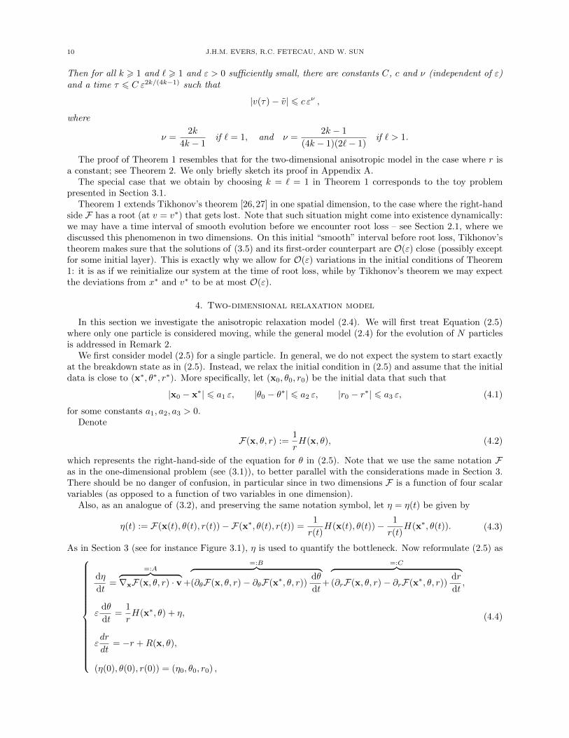
4. Two-dimensional relaxation model
In this section we investigate the anisotropic relaxation model (2.4). We will first treat Equation (2.5)where only one particle is considered moving, while the general model (2.4) for the evolution of N particlesis addressed in Remark 2.
We first consider model (2.5) for a single particle. In general, we do not expect the system to start exactlyat the breakdown state as in (2.5). Instead, we relax the initial condition in (2.5) and assume that the initialdata is close to (x∗, θ∗, r∗). More specifically, let (x0, θ0, r0) be the initial data that such that
|x0 − x∗| 6 a1 ε, |θ0 − θ∗| 6 a2 ε, |r0 − r∗| 6 a3 ε, (4.1)
for some constants a1, a2, a3 > 0.Denote
F(x, θ, r) :=1
rH(x, θ), (4.2)
which represents the right-hand-side of the equation for θ in (2.5). Note that we use the same notation Fas in the one-dimensional problem (see (3.1)), to better parallel with the considerations made in Section 3.There should be no danger of confusion, in particular since in two dimensions F is a function of four scalarvariables (as opposed to a function of two variables in one dimension).
Also, as an analogue of (3.2), and preserving the same notation symbol, let η = η(t) be given by
η(t) := F(x(t), θ(t), r(t))−F(x∗, θ(t), r(t)) =1
r(t)H(x(t), θ(t))− 1
r(t)H(x∗, θ(t)). (4.3)
As in Section 3 (see for instance Figure 3.1), η is used to quantify the bottleneck. Now reformulate (2.5) as
dη
dt=
=:A︷ ︸︸ ︷∇xF(x, θ, r) · v+
=:B︷ ︸︸ ︷(∂θF(x, θ, r)− ∂θF(x∗, θ, r))
dθ
dt+
=:C︷ ︸︸ ︷(∂rF(x, θ, r)− ∂rF(x∗, θ, r))
dr
dt,
εdθ
dt=
1
rH(x∗, θ) + η,
εdr
dt= −r +R(x, θ),
(η(0), θ(0), r(0)) = (η0, θ0, r0) ,
(4.4)

SMALL INERTIA REGULARIZATION OF AN ANISOTROPIC AGGREGATION MODEL 11
where we have denoted
η0 = F(x0, θ0, r0)−F(x∗, θ0, r0) .
Note that the spatial variable x appears explicitly in the dynamics for η; its evolution is governed bydx/dt = v = r (cos θ, sin θ)T .
The main assumptions for H are
Assumption 2. Assume that H ∈ C2(R2 × R;R). Suppose there exist two constants θ > θ∗ > 0 such thatH satisfies
• H(x∗, θ) = 0, H(x∗, θ∗) = ∂θH(x∗, θ∗) = 0,
• ∂2θH(x∗, θ∗) > 0, ∂θH(x∗, θ) < 0,
• H(x∗, φ) > 0 for all φ ∈ (θ∗, θ).
Assumption 2 guarantees that there is a function h ∈ C(R) strictly positive on [θ∗, θ] such that
H(x∗, φ) = −h(φ) · (φ− θ∗)2(φ− θ) , h(φ) > h0 > 0 , φ ∈ [θ∗, θ] (4.5)
for some constant h0 > 0. The motivation for such an assumption on H was presented in Section 2.1 – seefor example the dash-dotted line in Figure 2.2.
The assumptions we make on the function R are very unrestrictive – see the statement of Theorem 2. Inparticular, we assume that it is a bounded function and also, that R(x∗, ·) is strictly positive at θ∗ and θ.
Our main goal for this paper is to justify the jump discontinuity of the velocity of the particle as ε→ 0.Although the velocity now has two components r and θ, the main dynamics of (4.4) is driven by the θ-
equation. Hence, we first show the jump of θ from θ∗ to θ within a time interval that vanishes with ε andthen show the jump of r induced by the jump of θ.
To show the transition of θ we follow a similar approach as for the toy problem (3.1). Taken into accountthe extra terms in system (4.4) compared to (3.1), we will divide the whole transition process into fourstages:
• Interval I: Within this interval, a bottleneck will form for θ. At the end of the interval, we have thatθ − θ∗ = O(ε1/3). The term A is strictly positive and dominates B. The main driving force in thedynamics for θ is η.
• Interval II: The second interval is a preparation for escaping the bottleneck. More specifically, atthe end of the second interval, θ will reach the state where θ − θ∗ = O(ε1/6). During this intervalA+B > 0. The main driving force for θ is 1
rH ∼ (θ − θ∗)2.• Interval III: At the end of the third interval, θ will escape from the bottleneck, because the initial state
prepared by Interval II is large enough. Hence, at the end of Interval III we will have θ− θ∗ = O(1).
• Interval IV: In this last time interval, the main driving force for θ is 1rH ∼ −(θ − θ). Consequently,
θ is attracted to the stable equilibrium point θ.
The characteristics of the four intervals are represented schematically in Figure 4.1. There we also add theorders of magnitudes of the intervals themselves.
To account for possibly different characteristics of the profile R(x∗, ·) between θ∗ and θ, we distinguishbetween the following two cases:
(RP) R(x∗, φ) > 0 for all φ ∈ [θ∗, θ]. The scenario in Figure 2.2 falls into this category; the grey line isstrictly positive. In this case, define
R0 :=1
2min
φ∈[θ∗,θ]R(x∗, φ) > 0 . (4.6)
(RN) There exists φ ∈ [θ∗, θ] such that R(x∗, φ) = 0. In this case define
ϕ∗ := inf{φ ∈ [θ∗, θ] : R(x∗, φ) = 0}, ϕ := sup{φ ∈ [θ∗, θ] : R(x∗, φ) = 0} ,
ω∗ = (θ∗ + ϕ∗)/2 , ω = (ϕ+ θ)/2 . (4.7)
If ϕ∗ 6= ϕ, then R(x∗, ·) may become negative in the intermediate interval and may even havemultiple subsequent positive and negative intervals. The first zero of R(x∗, ·) is at ϕ∗, the last zero

12 J.H.M. EVERS, R.C. FETECAU, AND W. SUN
0 τ1 τ2 τ3 τ4
I II III IV
O(ε2/3) O(ε2/3)−O(ε5/6) O(ε5/6)−O(ε) O(ε1−λ)
θ − θ∗ = O(ε) θ − θ∗ = O(ε1/3) θ − θ∗ = O(ε1/6)
θ − θ∗ = O(1)
θ − θ = O(1)
θ − θ = O(ε2/3)
Figure 4.1. Orders of magnitude of the four time intervals that constitute the transition layer identified inTheorem 2. The total length of the four intervals is O(ε2/3). Note that in Interval IV, the parameter λ > 0
is arbitrarily small. The evolution of θ is also indicated. It moves from an ε-neighbourhood of θ∗ at time
t = 0 to an ε2/3-neighbourhood of θ at time t = τ4.
θ∗
ϕ∗ ϕ
θω∗ ω
R(x∗, · )
Figure 4.2. Schematic illustration of R(x∗, ·) in the case (RN). The function R(x∗, ·) is strictly positive at
θ∗ and θ. The first and last zero of R(x∗, ·) within the interval [θ∗, θ] are denoted by ϕ∗ and ϕ, respectively.In general, ϕ∗ = ϕ may happen, when R(x∗, ·) only touches the horizontal axis. If ϕ∗ 6= ϕ, then R(x∗, ·)could be negative everywhere in (ϕ∗, ϕ), or have additional zeros. The picture shows the case in which
R(x∗, ·) has multiple zeroes between ϕ∗ and ϕ. The point ω∗ is halfway between θ∗ and ϕ∗, and likewise
the point ω is halfway between ϕ and θ.
is at ϕ. Also note that ω∗ and ω do not depend on ε; these are quantities that are O(1) away fromthe zeroes of R(x∗, ·) – see Figure 4.2 for an illustration. We also define1
R0 :=1
2min
φ∈[θ∗,ω∗]∪[ω,θ]R(x∗, φ) > 0. (4.8)
Our main theorem states
Theorem 2. Assume that H,R ∈ C2(R2 × R;R) and H satisfies Assumption 2. Assume moreover that
A∗ = ∇xF(x∗, θ∗, r∗) · v∗ > 0 , r∗ = R(x∗, θ∗) > 0 , R(x∗, θ) > 0 . (4.9)
Let (η, θ, r) be the solution to (4.4) whose initial data satisfy (4.1). Let there be a constant R > 0 largeenough such that
0 < r0 6 R , and |R(z, φ)| 6 R for all (z, φ) ∈ R2 × R . (4.10)
Then, for all ε > 0 sufficiently small, there exist three positive constants C1, C2 and c (independent of ε)and a time C1ε
2/3 6 τ 6 C2 ε2/3 such that
|θ(τ)− θ| 6 c ε2/3 .
1Since cases (RP) and (RN) are mutually disjoint, using the same notation R0 in (4.6) and (4.8) is consistent, and in fact
very convenient for the presentation.
SMALL INERTIA REGULARIZATION OF AN ANISOTROPIC AGGREGATION MODEL 13
Proof. The proof is divided into four steps according to the four intervals described above. The commonprocedures within each interval are:
Estimate of |x− x∗| , |r − r∗|, and the bounds for r ⇒ Estimate of η ⇒ Estimate of θ − θ∗ .
We only distinguish between the cases (RP) and (RN) in the fourth interval. Hence, unless otherwise noted,the two cases are treated simultaneously, and notation R0 can refer to either (4.6) or (4.8).
Step 1: Interval I (Formation of the bottleneck). Compared with setting the initial data exactly at (x∗, θ∗, r∗),the main extra difficulty that the initial perturbation introduces is that η may not be positive near t = 0.Hence θ may not be increasing starting from t = 0. We want to show that after an initial interval of orderO(ε2/3), θ − θ∗ becomes positive and of order O(ε1/3).
First we introduce some constants before explicitly defining Interval I. Let
B := B(x∗, 1)× B(θ∗, 1) (4.11)
and
D :=3
R0
(maxB|∂θR|+ 1
), C0 :=
8D
A∗+
1
D, (4.12)
where R0 is defined as in (4.6) or (4.8) and A∗ is given by (4.9). Note that D is strictly positive and hence,C0 is well-defined. Let
σ1 := sup{t : |θ(s)− θ∗| 6 ε1/3 for all s ∈ [0, t]}. (4.13)
Define the end-time τ1 of Interval I as
τ1 := min{σ1, C0 ε2/3} . (4.14)
Note that since initially we have |θ0 − θ∗| = O(ε), the length of Interval I is strictly positive as long as ε issmall enough.
Our main goal in Step 1 is to show that at the end-time t = τ1,
θ(τ1)− θ∗ = ε1/3 and r(t) > 0 for all t ∈ [0, τ1] . (4.15)
We start by showing the following bounds on [0, τ1] (recall upper bound R introduced in (4.10)):
|x(t)− x∗| 6 D1 ε2/3, 0 < R0 6 r(t) 6 R , |r(t)− r∗| 6 D2 ε
1/3 , (4.16)
where D1, D2 are some constants independent of ε that will be defined later.The upper bound for r can be derived from the r-equation. Indeed, the ODE for r in (4.4) yields the
inequality
εd|r|dt6 −|r|+ R .
Hence, by the assumption for the initial data r0 in (4.10), we have
|r(t)| 6 R (4.17)
for all t such that the solution exists. Therefore on Interval I,
|x(t)− x∗| 6 |x(t)− x0|+ |x0 − x∗| 6 R · C0 ε2/3 + a1 ε 6 D1 ε
2/3 , (4.18)
where the constant D1 is chosen as D1 = 2RC0. By (4.13) and (4.18), we know that (x(t), θ(t)) ∈ B fort ∈ [0, τ1] and ε sufficiently small; cf. (4.11). Thus for ε small enough,
|R(x(t), θ(t))−R(x∗, θ∗)| 6 maxB|∇xR| ·D1 ε
2/3 + maxB|∂θR| · ε1/3 6 D2ε
1/3 , (4.19)
where
D2 = maxB|∂θR|+ 1 . (4.20)
Since R(x∗, θ∗) > 2R0, the bound (4.19) implies that for ε sufficiently small,
R(x(t), θ(t)) > R0 , t ∈ [0, τ1] .
We also have r0 > R0 since
|r0 −R(x∗, θ∗)| = |r0 − r∗| 6 a3 ε .

14 J.H.M. EVERS, R.C. FETECAU, AND W. SUN
Therefore R0 is a subsolution to the r-equation which gives
r(t) > R0 , t ∈ [0, τ1] .
Now we estimate the size of |r(t)− r∗|. Observe that by (4.4) and (4.19),
εd
dt|r − r∗| 6 − |r − r∗|+ |R(x(t), θ(t))−R(x∗, θ∗)| 6 − |r − r∗|+D2ε
1/3 (4.21)
with the initial data satisfying
|r0 − r∗| 6 a3 ε 6 D2ε1/3 for ε small enough .
Therefore D2 ε1/3 is a supersolution to (4.21), which gives
|r(t)− r∗| 6 D2ε1/3 , t ∈ [0, τ1] .
We thus have verified all the bounds in (4.16).
Next we study the evolution of η on Interval I by estimating the three terms A,B,C on the right-handside of the η-equation. We will show that on Interval I the term A is dominant. First by the continuity ofA in x, θ and r together with (4.16) and (4.9), we have that
A(t) > A∗/2 > 0 for all t ∈ [0, τ1]. (4.22)
Meanwhile, on Interval I, H and η satisfy
|H(x, θ)| 6 |H(x∗, θ∗)|︸ ︷︷ ︸=0
+|∇xH(x∗, θ∗)| · |x− x∗|+ |∂θH(x∗, θ∗)|︸ ︷︷ ︸=0
·|θ − θ∗|
+
(max
α1+α2+α3=2maxB|∂α1x ∂α2
y ∂α3
θ H|)·
∑α1+α2+α3=2
(x− x∗)α1(y − y∗)α2(θ − θ∗)α3
(4.23)
and
|η(t)| = 1
r(t)|H(x(t), θ(t))−H(x∗, θ(t))| 6 1
R0maxB|∇xH| |x− x∗| . (4.24)
Since |x(t)− x∗| 6 D1 ε2/3 and |θ(t)− θ∗| 6 ε1/3 on Interval I, it follows from (4.23) and (4.24) that
|η(t)| 6 D3 ε2/3 , |H(x(t), θ(t))| 6 D4 ε
2/3 , t ∈ [0, τ1] , (4.25)
and
|∂θH(x(t), θ(t))− ∂θH(x∗, θ(t))| 6 maxB|∇x∂θH| · |x(t)− x∗| 6 D5 ε
2/3 t ∈ [0, τ1] , (4.26)
where D3, D4, D5 are positive constants that are independent of ε. We can then estimate |B(t)| using (4.16),(4.25) and (4.26) and obtain that
|B(t)| 6∣∣∣∣ 1
r(t)∂θH(x(t), θ(t))− 1
r(t)∂θH(x∗, θ(t))
∣∣∣∣ · 1
ε
∣∣∣∣ 1
r(t)H(x∗, θ(t)) + η(t)
∣∣∣∣6
1
εR20
(D5 ε2/3) (D4 +R0D3) ε2/3 6
D5 (D4 +R0D3)
R20
ε1/3 .
(4.27)
Hence, for sufficiently small ε, it holds that |B(t)| 6 A∗/4. Together with (4.22) we have
A(t) +B(t) > A∗/4 , t ∈ [0, τ1] . (4.28)
Regarding the term C, we note that
C =
(∂rF(x, θ, r)− ∂rF(x∗, θ, r)
)dr
dt=
(− 1
r2H(x, θ) +
1
r2H(x∗, θ)
)dr
dt= −1
rη
dr
dt.
Denote
G(t) :=1
r(t)
dr
dt. (4.29)
SMALL INERTIA REGULARIZATION OF AN ANISOTROPIC AGGREGATION MODEL 15
Then for every t ∈ [0, τ1], by (4.16), (4.20) and the definition of Interval I we have
|G(t)| =∣∣∣∣ 1
r(t)
dr
dt
∣∣∣∣ =1
ε
1
r(t)·∣∣− r(t) +R(x(t), θ(t)) + r∗ −R(x∗, θ∗)︸ ︷︷ ︸
=0
∣∣6
1
εR0
(|r(t)− r∗|+ max
B|∇xR| · |x(t)− x∗|+ max
B|∂θR| · |θ(t)− θ∗|
)6
1
εR0
(D2 ε
1/3 + maxB|∇xR| ·D1 ε
2/3 +D2 ε1/3
)6
3D2
R0ε−2/3 , t ∈ [0, τ1] . (4.30)
Combining (4.28) with (4.30), we thus have on Interval I,
dη
dt>
1
4A∗ −G · η > 1
4A∗ − 3D2
R0ε−2/3η . (4.31)
Meanwhile, the initial data η(0) satisfies
|η(0)| =∣∣∣∣ 1
r0H(x0, θ0)− 1
r0H(x∗, θ0)
∣∣∣∣ 6 1
r0max
x∈B(x∗,1)|∇xH(x, θ0)| · |x0 − x∗|︸ ︷︷ ︸
6a1 ε
6 D6 ε, (4.32)
where D6 = a1R0
maxB |∇xH|.Recall the definition of D in (4.12) and solve (4.31) together with (4.32). This yields that
η(t) > −D6 ε+A∗
4L(ε)
(1− exp
(− L(ε) t
)), L(ε) = Dε−2/3 . (4.33)
Note that, by Assumption 2, we have that H(x∗, θ(t)) > 0 on Interval I, for ε sufficiently small. Hence
εdθ
dt= η +
1
rH(x∗, θ) > η . (4.34)
thus it follows from (4.33) that
θ(t)− θ∗ > θ0 − θ∗︸ ︷︷ ︸>−a2 ε
+
(A∗
4 εL(ε)−D6
)t+
A∗
4 ε (L(ε))2
(exp(−L(ε) t)− 1
). (4.35)
At the end of Interval I, either of the following two cases is true:
Case I-1: the end of Interval I is reached when θ(τ1) − θ∗ = ε1/3. By (4.13), we know that the finaltime must satisfy τ1 6 C0 ε
2/3.Case I-2: the end of Interval I is reached when θ(τ1) − θ∗ = −ε1/3. Substituting the inequality
exp(−z) > 1− z in (4.35), we then find that
−ε1/3 = θ(τ1)− θ∗ > −a2 ε−D6 τ1
must hold in this case. This implies, for ε sufficiently small, that
τ1 >1
2D6ε1/3,
which contradicts the assumption that τ1 6 C0 ε2/3. Therefore at the end of Interval I it can not
happen that θ(τ1)− θ∗ = −ε1/3.Case I-3: the end of Interval I is reached when τ1 = C0 ε
2/3. Note that, by the definition of L(ε)in (4.33), we have
A∗
4 εL(ε)=
A∗
4Dε1/3,
A∗
4 ε (L(ε))2=A∗ ε1/3
4D2,
Therefore
A∗
4 εL(ε)−D6 > 0 for ε small enough.
Hence by (4.35) we have
θ(τ1)− θ∗ > −a2 ε+
(A∗
4 εL(ε)−D6
)· C0 ε
2/3 − A∗
4 ε (L(ε))2. (4.36)

16 J.H.M. EVERS, R.C. FETECAU, AND W. SUN
By the definitions of C0 and D in (4.12), we have
A∗ C0
4D− A∗
4D2= 2 .
Hence, (4.36) implies that
θ(τ1)− θ∗ >(A∗ C0
4D− A∗
4D2
)· ε1/3 − a2 ε−D6C0 ε
2/3
= 2 ε1/3 − a2 ε−D6C0 ε2/3 > ε1/3.
The latter inequality holds for ε sufficiently small. Rather than just θ(τ1)− θ∗ > ε1/3, actually theequality θ(τ1)− θ∗ = ε1/3 must hold, since otherwise τ1 would have been reached before t = C0 ε
2/3.
In conclusion, at the end of Interval I we have that
τ1 6 C0 ε2/3 and θ(τ1)− θ∗ = ε1/3.
We also have estimates for η at the end-time τ1. First, by (4.25), we have
dθ
dt6
1
ε
∣∣∣∣1rH + η
∣∣∣∣ 6 1
εR0(D4 +R0D3) ε2/3 6
1
R0(D4 +R0D3) ε−1/3 .
Integrating from 0 to τ1 gives
ε1/3 = θ(τ1)− θ∗ 6 θ0 − θ∗ +1
R0(D4 +R0D3) ε−1/3τ1 6 a2ε+
1
R0(D4 +R0D3) ε−1/3τ1 .
Therefore for ε small enough, we derive that
τ1 >R0
2 (D4 +R0D3)ε2/3 . (4.37)
It can be shown that the constant in this lower bound is smaller than C0 (details are left to the reader),hence there is no inconsistency with the upper bound τ1 6 C0 ε
2/3. Substitution in (4.33) of the lower boundof τ1, gives
η(τ1) > −D6 ε+A∗
4D
(1− exp
(− DR0
2 (D4 +R0D3)
))ε2/3 > 0 for ε small enough. (4.38)
Step 2: Interval II (Preparation for escaping the bottleneck). Within this interval, we show that θ movesfurther away from θ∗. This will provide a large enough initial data for Interval III, during which θ attainsan order O(1) distance from θ∗, thus escaping the bottleneck. The main difference of the analysis betweenInterval I and II is that now we will use 1
rH as the main driving force for the evolution of θ as opposed to ηused in Interval I.
We define the end-time of Interval II as follows. Let α > 0 be a ‘sufficiently small’ parameter (detailsfollow later) that is independent of ε, and let
σ2 := sup{t > τ1 : ε1/3 6 θ(s)− θ∗ 6 α ε1/6 for all s ∈ [τ1, t]} .
The end-time for Interval II is defined as
τ2 := min{σ2, τ1 + C1 ε2/3 − C2 ε
5/6} , (4.39)
where the constants are
C1 :=2R(
minφ∈[θ∗,θ] h(φ))· (θ − θ∗)
, C2 :=C1
α. (4.40)
The function h is as given in (4.5), and R is as in (4.10). We have from (4.38) that η(τ1) > 0 and,consequently, dθ/dt > 0 at time t = τ1 due to (4.34). Moreover, θ(τ1)− θ∗ = ε1/3. Therefore it must holdthat σ2 > τ1 and the length of the interval [τ1, τ2] (i.e. Interval II) is strictly positive, provided that ε issufficiently small.
Our main goal for Interval II is to show that
θ(τ2)− θ∗ = α ε1/6 and r(t) > 0 for all t ∈ [τ1, τ2] . (4.41)

SMALL INERTIA REGULARIZATION OF AN ANISOTROPIC AGGREGATION MODEL 17
The first estimate on Interval II is similar to that in Interval I. In particular, we want to show that withinInterval II:
|x(t)− x∗| 6 D7 ε2/3, 0 < R0 6 r(t) 6 R , |r(t)− r∗| 6 D8 ε
1/6 , (4.42)
where R0, R are defined in (4.6) or (4.8) and (4.10) and D7, D8 are some constants independent of ε. Thederivation of the bounds for x(t) and r(t) in (4.42) is similar to Interval I. In particular, by the bound of rin (4.17), given that the combined lengths of the intervals I and II is smaller than (C0 + C1)ε2/3, we have
|x(t)− x∗| 6 R(C0 + C1) ε2/3 := D7 ε2/3. (4.43)
Analogously to (4.19), we find that
|R(x(t), θ(t))− r∗| 6 D8 ε1/6 , t ∈ [τ1, τ2] ,
where D8 := D7 ·maxB |∇xR|+ α maxB |∂θR|. Subsequently, an argument like (4.21) yields that
|r(t)− r∗| 6 D8 ε1/6 .
Therefore all the bounds in (4.42) hold. These bounds imply, like in (4.22), that for ε small enough,
A(t) > A∗/2 , t ∈ [τ1, τ2] ,
Now we show that η remains non-negative on Interval II. Using a Taylor expansion comparable to (4.23),we find that
|H(x, θ)| 6 D9 ε2/3 +D10 α
2 ε1/3, (4.44)
where D10 := maxB |∂2θH|, and D9 depends on a number of first- and second-order partial derivatives of H.
Note that if we restrict ourselves to ε 6 1 and α 6 1, then D9 can be taken such that it is independent of αand ε. Moreover, a similar argument as in (4.26) gives
|∂θH(x, θ)− ∂θH(x∗, θ)| 6 D7 ·maxB|∇x∂θH|︸ ︷︷ ︸
=:D11
· ε2/3, (4.45)
Due to (4.44) and (4.45), we have the following analogue of (4.27):
|B(t)| 6 1
εR20
·D11 ε2/3 · (D9 ε
2/3 +D10 α2 ε1/3 +D7 max
B|∇xH| ε2/3)
=D11D9
R20
ε1/3 +D11D10
R20
α2 +D11D7 maxB |∇xH|
R20
ε1/3 ,
where we also used (4.24) and (4.43) to bound |η|. Consequently, |B(t)| 6 A∗/2 on Interval II, if ε and αare sufficiently small. The choice of α is in particular independent of ε. Such choice of α gives
A(t) +B(t) > 0 , t ∈ [τ1, τ2] . (4.46)
The lower bound (4.46) is not sharp but nevertheless sufficient for the analysis in the sequel. By (4.46), thefunction η satisfies the inequality
dη
dt> C(t) = −G(t) · η ,
where C(t), G(t) are defined in (4.4) and (4.29). The initial data η(τ1) is positive due to (4.38). Therefore,
η(t) > η(τ1) · exp(−∫ t
τ1
G(s) ds) > 0 , t ∈ [τ1, τ2] .
Using the positivity of η on Interval II, we can now show the first equality in (4.41). Since θ is arbitrarilyclose to θ∗ for ε sufficiently small, we have that H(x∗, θ) > 0 on Interval II. Hence,
εdθ
dt= η︸︷︷︸
>0
+1
rH(x∗, θ)︸ ︷︷ ︸
>0
> 0,
and thus θ is increasing in Interval II. Moreover, for ε sufficiently small, we have
θ − θ(t) > (θ − θ∗)/2 , t ∈ [τ1, τ2] .
18 J.H.M. EVERS, R.C. FETECAU, AND W. SUN
Hence, since η is positive and by the definition of C1 in (4.40), the θ-equation satisfies
εdθ
dt>
1
R
(min
φ∈[θ∗,θ]h(φ)︸ ︷︷ ︸
>0
)· 1
2(θ − θ∗) · (θ(t)− θ∗)2 =
1
C1(θ(t)− θ∗)2 . (4.47)
This yields the differential inequality
d
dt(θ − θ∗) > 1
C1 ε(θ − θ∗)2 , θ(τ1)− θ∗ = ε1/3 . (4.48)
Solving (4.48) then gives
θ(t)− θ∗ > ε
ε2/3 − 1C1
(t− τ1), t ∈ [τ1, τ2] . (4.49)
Since θ(·) is nondecreasing, it cannot leave the interval [θ∗ + ε1/3, θ∗ + α ε1/6] at its left-hand boundary. Atthe end of Interval II, one of the following is therefore satisfied:
Case II-1: θ(τ2) − θ∗ = α ε1/6. By (4.39), we know that the final time must satisfy τ2 − τ1 6C1 ε
2/3 − C2 ε5/6.
Case II-2: τ2 − τ1 = C1 ε2/3 − C2 ε
5/6. It follows from (4.49) that,
θ(τ2)− θ∗ > α ε1/6,
due to our choice of C1 and C2. In fact, θ(τ2)− θ∗ must be equal to α ε1/6, since otherwise τ2 wouldhave been reached before t = τ1 + C1 ε
2/3 − C2 ε5/6.
Together with the bounds of r in (4.42), we have shown that (4.41) holds at the end of Interval II.
Step 3: Interval III (Escape from the bottleneck). In this part we show that within a time interval of length
O(ε5/6
)after Interval II, θ will escape from the bottleneck and become order O(1) away from θ∗.
We characterize the distance from θ to θ∗ by a parameter β ∈ (0, 1). More specifically, if (RN) holds,then let the parameter 0 < β < 1 be sufficiently small, such that
θ∗ + β (θ − θ∗) 6 ω∗ .Recall that ω∗ was defined in (4.7), such that it is smaller than the first zero of R(x∗, ·); cf. Figure 4.2. If(RP) holds, then let β be an arbitrary parameter such that 0 < β < 1. Such choice of β guarantees in bothcases (RN) and (RP) that
R(t) > 2R0 , in Interval III. (4.50)
To define the end-time for Interval III, we first introduce the constants
C3 :=C1
α (1− β), C4 :=
C1
β (1− β)(θ − θ∗), (4.51)
with C1 defined in (4.40). Let
σ3 := sup{t > τ2 : α ε1/6 6 θ(s)− θ∗ 6 β (θ − θ∗) for all s ∈ [τ2, t]} . (4.52)
Then the end-time of Interval III is defined as
τ3 := min{σ3, τ2 + C3 ε5/6 − C4 ε}. (4.53)
Observe that by evaluating (4.48) at t = τ2 and noting that θ(τ2) − θ∗ = α ε1/6, we obtain that dθ/dt > 0at t = τ2. Therefore σ3 > τ2 and the length of Interval III, i.e. the interval [τ2, τ3], is strictly positive.
The main goal in this part is to show that
θ(τ3)− θ∗ = β (θ − θ∗) , and r(t) > 0 , t ∈ [τ2, τ3] . (4.54)
First, a similar argument as for Interval I and II shows that by our choice of β and (4.50),
|x(t)− x∗| 6 R (C0 + C1 + C3) ε2/3 , R0 6 r(t) 6 R , t ∈ [τ2, τ3] . (4.55)
To estimate the rate of growth of θ we need an appropriate bound for η. Unlike the estimates for ηin Interval I and II, where we carefully compared the sizes of A and B, now we only need a rather crudeestimate following directly from the definition in (4.3). First, for ε small enough, we know that
(x(t), θ(t)) ∈ B′ , t ∈ [τ2, τ3],
SMALL INERTIA REGULARIZATION OF AN ANISOTROPIC AGGREGATION MODEL 19
whereB′ := B(x∗, 1)× B(θ∗, θ − θ∗) . (4.56)
Therefore by definition of η in (4.3), it follows that
|η(t)| 6 1
R0maxB′|∇xH| · |x(t)− x∗|. (4.57)
Combining (4.55) with (4.57), we have
|η(t)| 6 D12 ε2/3, (4.58)
with D12 := R/R0 · (C0 + C1 + C3) ·maxB′ |∇xH|, which is independent of ε.Using the bound for η, now we study the evolution of θ − θ∗. By (4.52):
θ∗ + α ε1/6 6 θ(t) 6 θ∗ + β (θ − θ∗) , t ∈ [τ2, τ3] .
In particular, θ(t) ∈ [θ∗, θ] and θ − θ(t) > (1− β) · (θ − θ∗). For the evolution of θ we have,
εd(θ − θ∗)
dt>
1
R
(min
φ∈[θ∗,θ]h(φ)
)· (1− β) (θ − θ∗) · (θ(t)− θ∗)2 + η(t). (4.59)
This estimate is similar to (4.47), be it that η is no longer nonnegative. Instead, we know that η(t) >−D12 ε
2/3, due to (4.58). If we define
D13 :=2(1− β)
C1,
with C1 given by (4.40), then D13 is exactly the coefficient in front of (θ − θ∗)2 in (4.59). Hence, it followsfrom (4.59) that
εd(θ − θ∗)
dt> D13(θ − θ∗)2 −D12 ε
2/3.
Consequently, the θ-equation satisfies
d(θ − θ∗)dt
>1
2D13 ε
−1 (θ − θ∗)2 +1
2D13 α
2 ε−2/3 −D12 ε−1/3︸ ︷︷ ︸
> 0 for ε sufficiently small
>1
2D13 ε
−1 (θ − θ∗)2 , (4.60)
for all t ∈ [τ2, τ3]. Here, we used that (θ − θ∗) > α ε1/6. The accompanying initial condition is θ(τ2)− θ∗ =α ε1/6. After solving for the corresponding subsolution, we find that
θ(t)− θ∗ > 2α ε
2 ε5/6 − αD13 (t− τ2). (4.61)
Since θ is increasing within Interval III, at the end of the interval, there are only two possible scenarios:
Case III-1: θ(τ3) − θ∗ = β (θ − θ∗). By (4.53), we know that the final time must satisfy τ3 − τ2 6C3 ε
5/6 − C4 ε.Case III-2: τ3 − τ2 = C3 ε
5/6 − C4 ε. It follows from (4.61) that
θ(τ3)− θ∗ > 2α ε
2 ε5/6 − αD13 (C3 ε5/6 − C4 ε)= β (θ − θ∗),
by the definitions of C3, C4 in (4.51). This lower bound implies that θ(τ3) − θ∗ must actually be
equal to β (θ − θ∗), since otherwise τ3 would have been reached before t = τ2 + C3 ε5/6 − C4 ε.
It follows from the above considerations that (4.54) holds on Interval III.
Step 4: Interval IV (Convergence to θ). In this last interval we show that θ converges to θ. The rough
definition of the endpoint of Interval IV is the time when θ falls into a small neighbourhood of θ. The mainidea is that the first term 1
rH on the right-hand side of the θ-equation becomes a linear forcing that drives
θ toward θ. However, unlike in the previous three intervals, we have to treat separately the case (RN), asthe forcing term R in the r-equation may become negative in Interval IV. This generates a delicate situationregarding the positivity of r.
Case (RN) In this case R is bounded but is allowed to be negative for θ ∈ [ω∗, ω]; see Figure 4.2. We willshow however that r remains strictly positive. To this end, we divide Interval IV into two subintervals IV-Aand IV-B: during the first subinterval IV-A, θ evolves from θ(τ3) to ω, thus covering the whole region where

20 J.H.M. EVERS, R.C. FETECAU, AND W. SUN
R can be negative. This is the region where we need to estimate r carefully and show that it remains strictlypositive. During the second subinterval θ satisfies θ > ω. Hence, R has a strict lower bound which makesthe analysis more straightforward.
We start by giving the precise definition of the first subinterval IV-A. Let
σ4A := sup{t > τ3 : θ∗ + β (θ − θ∗) 6 θ(s) 6 ω and r(s) > 0 for all s ∈ [τ3, t]}, (4.62)
Define the end-time τ4A of the first subinterval IV-A as
τ4A := min{σ4A, τ3 + C5 ε}, (4.63)
where
C5 :=R
D14
(ω − θ∗ − β (θ − θ∗)
)> 0 , D14 :=
1
2min
φ∈[θ∗+β (θ−θ∗) , ω]H(x∗, φ) > 0. (4.64)
Since θ(τ3) − θ∗ = β (θ − θ∗), (4.60) implies that dθ/dt > 0 at t = τ3. Moreover, r(τ3) > R0 > 0. Hence,cf. (4.62), it holds that σ4A > τ3 and the length of Interval IV-A is strictly positive. Our main objective for
Interval IV-A is to show that there exists a constant R0 > 0 such that
θ(τ4A) = ω , 0 < R0 6 r(t) 6 R , t ∈ [τ3, τ4A] . (4.65)
The upper bound r 6 R holds for all t > 0, while by the definition of τ4A we have r > 0 for t ∈ [τ3, τ4A).Consequently,
|x(t)− x∗| 6 R (C0 + C1 + C3) ε2/3 + R C5 ε , t ∈ [τ3, τ4A] . (4.66)
DefineR := 2 max
φ∈[θ∗,θ](−R(x∗, φ))︸ ︷︷ ︸
> 0 in case (RN)
+1 > 0 .
The reason for adding 1 in the above definition is to make sure that R > 0 rather than R > 0, which turnsout to be useful in the sequel. Then
R(x∗, θ(t)) > −R/2 , t ∈ [0, τ4A] . (4.67)
Due to (4.66), the difference between R(x(t), θ(t)) and R(x∗, θ(t)) is arbitrarily small (for sufficiently smallε). Hence, it follows from (4.67) that
R(x(t), θ(t)) > −R , t ∈ [τ3, τ4A] ,
provided ε is sufficiently small. In order to show the positive lower bound of r, we study the rate of changeof r with respect to θ. Note that (x(t), θ(t)) ∈ B′ within Interval IV-A, with B′ being defined in (4.56). By(4.66) and the definition of η in (4.3), we have
|η(t)| 6 1
r(t)maxB′|∇xH| · |x(t)− x∗| 6 1
r(t)maxB′|∇xH| · R · (C0 + C1 + C3 + C5) ε2/3. (4.68)
Furthermore,1
r(t)H(x∗, θ(t)) >
1
r(t)min
φ∈[θ∗+β (θ−θ∗) , ω]H(x∗, φ) > 0 , t ∈ [τ3, τ4A)
with the lower bound being strictly positive due to (4.5). By (4.68) η is arbitrarily small for ε sufficientlysmall, and hence we have (for ε small enough) that
εdθ
dt=
1
r(t)H(x∗, θ(t)) + η(t) >
D14
r(t)> 0 , t ∈ [τ3, τ4A) , (4.69)
where the positive constant D14 is given by (4.64). The evolution of r, on the other hand, satisfies
εdr
dt= −r +R(x, θ) > −(r + R) (4.70)
with r + R > 0. Combining (4.69) and (4.70), we have
dr
dθ=ε
dr
dt
εdθ
dt
>−(r + R)
εdθ
dt
>−r(r + R)
D14,

SMALL INERTIA REGULARIZATION OF AN ANISOTROPIC AGGREGATION MODEL 21
where the right-hand side is strictly negative. Hence we have
dr
r(r + R)=
1
R
(1
r− 1
r + R
)dr > − dθ
D14.
Integration of this differential inequality from τ3 to some t ∈ [τ3, τ4A] yields
ln
(r(t)
r(τ3)
)− ln
(r(t) + R
r(τ3) + R
)> − R
D14(θ(t)− θ(τ3))
from which it follows that
r(t) >R(
1 + R/r(τ3))· exp
(R · (θ(t)− θ(τ3))/D14
)− 1
, t ∈ [τ3, τ4A) . (4.71)
By (4.69), we know that θ is strictly increasing on Interval IV-A. Hence θ(t) > θ(τ3) for t ∈ [τ3, τ4A] and theright-hand side of (4.71) is strictly positive. Furthermore, by (4.54) and (4.55), we know that R0 6 r(τ3) 6 R,
θ(τ3) = θ∗ + β (θ − θ∗); also, θ(t) ∈ [θ∗ + β (θ − θ∗) , ω] on Interval IV-A. Hence,
r(t) > R0 :=R0 R
R0 + R· exp
(−R (ω − θ∗)/D14
)> 0 , t ∈ [τ3, τ4A] . (4.72)
Therefore, the second bound in (4.65) holds and the end of Interval IV-A cannot be due to r reaching zero.To show the first equality in (4.65), we derive from (4.69) that
θ(t) > θ∗ + β (θ − θ∗) +D14 (t− τ3)
ε R, t ∈ [τ3, τ4A] (4.73)
Since θ is increasing, the end of Interval IV-A is reached in either of the following two cases:
Case IV-1: θ(τ4A) = ω. By (4.63), we know that the final time must satisfy τ4A − τ3 6 C5 ε.Case IV-2: τ4A − τ3 = C5 ε. Therefore, due to (4.73), it holds at time τ4A that
θ(τ4A) > θ∗ + β (θ − θ∗) +D14 C5
R= ω,
where the last equality follows from the definition of C5 in (4.64). Thus, θ(τ4A) = ω must hold, sinceotherwise the end of Interval IV-A would have been reached earlier than at τ4A.
We thereby have shown that (4.65) holds.
Next, we define the second subinterval IV-B. Let λ be an arbitrary constant such that 0 < λ 6 1/3 andfix n ∈ N such that nλ > 2/3. Define
σ4B := sup{t > τ4A : ω 6 θ(s) 6 θ − c ε2/3 for all s ∈ [τ4A, t]}, (4.74)
The end-time of the subinterval IV-B is defined by
τ4B := min{σ4B , τ4A + C6 ε1−λ}, (4.75)
with
C6 :=R (n! (θ − ω))1/n
(ω − θ∗)2 ·minφ∈[θ∗,θ] h(φ), c = 1 +
R2 (C0 + C1 + C3 + C5 + C6) ·maxB′ |∇xH|R0 (ω − θ∗)2 ·minφ∈[θ∗,θ] h(φ)
, (4.76)
where R0 = min{R0, R0} with R0 being the lower bound of r on IV-A defined in (4.72). Since θ(τ4A) = ωand dθ/dt > 0 at time τ4A, it holds that σ4B > τ4A. Consequently, τ4B > τ4A and the time-length ofthe subinterval IV-B is strictly positive. The introduction of the arbitrary number λ will be clear from theanalysis below.
Our main goal on Interval IV-B is to show that
θ(τ4B) = θ − c ε2/3 , r(t) > R0 = min{R0, R0} , t ∈ [τ4A, τ4B ] . (4.77)
Similar as in all the previous intervals, the upper bound (4.17) holds for all t > 0. Consequently,
|x(t)− x∗| 6 R · (C0 + C1 + C3 + C5 + C6) ε2/3 , t ∈ [0, τ4B ] (4.78)

22 J.H.M. EVERS, R.C. FETECAU, AND W. SUN
where we use that λ 6 1/3. Due to (4.8) and (4.74) we have that R(x∗, θ(t)) > 2R0 for all t ∈ [τ4A, τ4B ],and therefore
r(t) > R0 = min{R0, R0} > 0 , t ∈ [0, τ4B ] .
Compare the way in which we derived the lower bounds on r in (4.16), (4.42), (4.55) and (4.65). Hence thelower bound for r in (4.77) holds.
In order to show the first equality in (4.77), we again use the definition of η and obtain its bound as
|η(t)| 6 D15 ε2/3 , t ∈ [τ4A, τ4B ] . (4.79)
where the constant D15 is given by
D15 := R/R0 · (C0 + C1 + C3 + C5 + C6) ·maxB′|∇xH| . (4.80)
Using the above bound of η, we have
εd(θ − θ)
dt> −D16 (θ(t)− θ)−D15 ε
2/3 , (4.81)
whereD16 := (ω − θ∗)2/R · min
φ∈[θ∗,θ]h(φ). (4.82)
Note that (4.76), (4.80) and (4.82) imply that c = 1 +D15/D16. The initial condition θ(τ4A)− θ = ω− θ < 0
is an O(1)-quantity, while θ − θ(t) > c ε2/3 on Interval IV-B due to (4.74). Therefore, for any ε sufficientlysmall, the right-hand side of (4.81) is strictly positive for all t in Interval IV-B, and thus θ is increasing.
Moreover, the subsolution of (4.81) corresponding to the initial condition θ(τ4A)− θ leads to the lower bound:
θ(t)− θ > −D15
D16ε2/3 +
(D15
D16ε2/3 − (θ − ω)
)· exp(−D16 (t− τ4A)/ε). (4.83)
Since θ is increasing, the end of Interval IV-B is reached in either of the following two cases:
Case IV-3: θ(τ4B) = θ − c ε2/3. By (4.75), we know that the final time must satisfy τ4B − τ4A 6C6 ε
1−λ.Case IV-4: τ4B − τ4A = C6 ε
1−λ. The lower bound in (4.83) implies that
θ(τ4B)− θ > − D15
D16ε2/3 +
(D15
D16ε2/3 − (θ − ω)
)· exp(−D16 C6 ε
−λ) (4.84)
> − D15
D16ε2/3 − (θ − ω) · exp(−D16 C6 ε
−λ). (4.85)
For each w > 0 and γ ∈ N, the inequality exp(w) > 1 + wγ/γ! holds. Hence,
exp(−D16 C6 ε−λ) 6
1
1 + (D16 C6)n ε−nλ/n!=
n! εnλ
n! εnλ + (D16 C6)n6
n! ε2/3
(D16 C6)n, (4.86)
where we used in the last inequality that nλ > 2/3. Note that D16 C6 = (n! (θ − ω))1/n, by (4.76)and (4.82). Consequently, (4.85) and (4.86) combine into
θ(τ4B)− θ > −(
1 +D15
D16
)ε2/3 = −c ε2/3,
since c = 1 +D15/D16, as stated before. Thus, θ(τ4B)− θ = −c ε2/3 must hold, since otherwise theend of Interval IV-B would have been reached earlier than at τ4B .
We thereby have shown that |θ(τ4B)− θ| = c ε2/3, while τ4B 6 (C0 +C1 +C3 +C5 +C6) ε2/3. Furthermore,τ4B > τ1 > C1 ε
2/3, where the constant C1 is provided by (4.37). Hence the statement of the theorem isproved in the case (RN).
Case (RP) This case is a repetition of the analysis in Inteval IV-B for the (RN) case, since now weautomatically have
r(t) > R0 > 0 .
Therefore it is not necessary to subdivide Interval IV into two subintervals. We nevertheless present somedetails for the convenience of the reader.
SMALL INERTIA REGULARIZATION OF AN ANISOTROPIC AGGREGATION MODEL 23
Let λ be an arbitrary constant such that 0 < λ 6 1/3 and let n ∈ N be such that nλ > 2/3. Define
σ4 := sup{t > τ3 : θ∗ + β (θ − θ∗) 6 θ(s) 6 θ − c ε2/3 for all s ∈ [τ3, t]}, (4.87)
and the end-time τ4 of Interval IV as
τ4 := min{σ4, τ3 + C7 ε1−λ} , (4.88)
with
C7 :=C1 (n! (1− β) (θ − θ∗))1/n
2β2 (θ − θ∗), c := 1 +
C1
(D12 + C7 R/R0 ·maxB′ |∇xH|
)2β2 (θ − θ∗)
.
Together with θ(τ3)− θ∗ = β (θ− θ∗), (4.60) implies that dθ/dt > 0 at t = τ3. Hence, it holds that σ4 > τ3.Using similar arguments as before, we can show that 0 < R0 6 r(t) 6 R is satisfied within Interval IV.Moreover, |x(t) − x∗| has an upper bound of order O(ε2/3); this can be proved analogously to e.g. (4.78).Consequently, we have due to (4.57) that
|η(t)| 6 D17 ε2/3
for all t ∈ [τ3, τ4]. Here, D17 := D12 + R/R0 · C7 ·maxB′ |∇xH|. The estimate of η is very similar to (4.58),be it that the constant D17 takes into account the appropriate estimate for |x(t)− x∗| in this interval.
By definition of σ4, we have that θ(t)− θ∗ > β (θ− θ∗) on Interval IV. Hence, like in (4.81), we have that
εd(θ − θ)
dt> −D18 (θ(t)− θ)−D17 ε
2/3 (4.89)
holds in Interval IV, with D18 = 2β2 (θ − θ∗)/C1. The initial condition is θ(τ3) − θ = −(1 − β) · (θ − θ∗).Now, we follow the same steps as in Interval IV-B for the case (RN). The end of Interval IV is reached ineither of the following two cases:
Case 1: θ(τ4) = θ − c ε2/3. By (4.88), we know that the final time must satisfy τ4 − τ3 6 C7 ε1−λ.
Case 2: τ4 − τ3 = C7 ε1−λ. Due to the same arguments as in Interval IV-B of (RN), and using the
definitions of C7 = (n! (1− β) (θ − θ∗))1/n/D18 and c = 1 +D17/D18, we obtain that
θ(τ4)− θ > −c ε2/3.
Thus, |θ(τ4)− θ| = c ε2/3 must hold, since otherwise the end of Interval IV would have been reachedearlier than at τ4.
We have shown that |θ(τ4)−θ| = c ε2/3, while τ4 6 (C0+C1+C3+C7) ε2/3. Furthermore, τ4B > τ1 > C1 ε2/3,
where the constant C1 is provided by (4.37). Hence the statement of the theorem is proved also for the case(RP). �
Remark 1. Let ζ be an O(1) quantity such that R(x∗, ·) is strictly positive on (θ∗ − ζ, θ∗]. Such ζ exists bythe continuity of R(x∗, ·) and the positivity of R(x∗, θ∗). Then for each fixed ε, the well-posedness of (4.4)
over the time period when θ ∈ (θ∗ − ζ, θ) immediately follows from the bounds (both lower and upper) of rand θ shown in the proof of Theorem 2.
Next we show that, provided R is not a constant on [θ∗, θ], the speed r also experiences a finite jump;compare Figure 2.3(c). The jump in r is generated by the jump of θ shown in the previous theorem. Themain idea here is: R undergoes a finite jump that is induced by the jump of θ. This further translatesinto the jump of r. Back to the particle description, this indicates that both the speed and direction of theparticle make an instantaneous change as ε → 0. This is the procedure that picks up the correct state forthe first-order model.
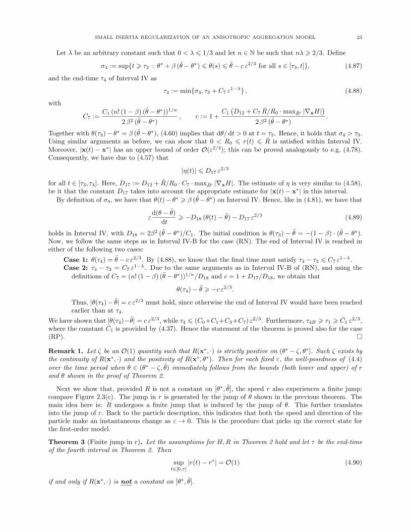
Theorem 3 (Finite jump in r). Let the assumptions for H,R in Theorem 2 hold and let τ be the end-timeof the fourth interval in Theorem 2. Then
supt∈[0,τ ]
|r(t)− r∗| = O(1) (4.90)
if and only if R(x∗, ·) is not a constant on [θ∗, θ].
24 J.H.M. EVERS, R.C. FETECAU, AND W. SUN
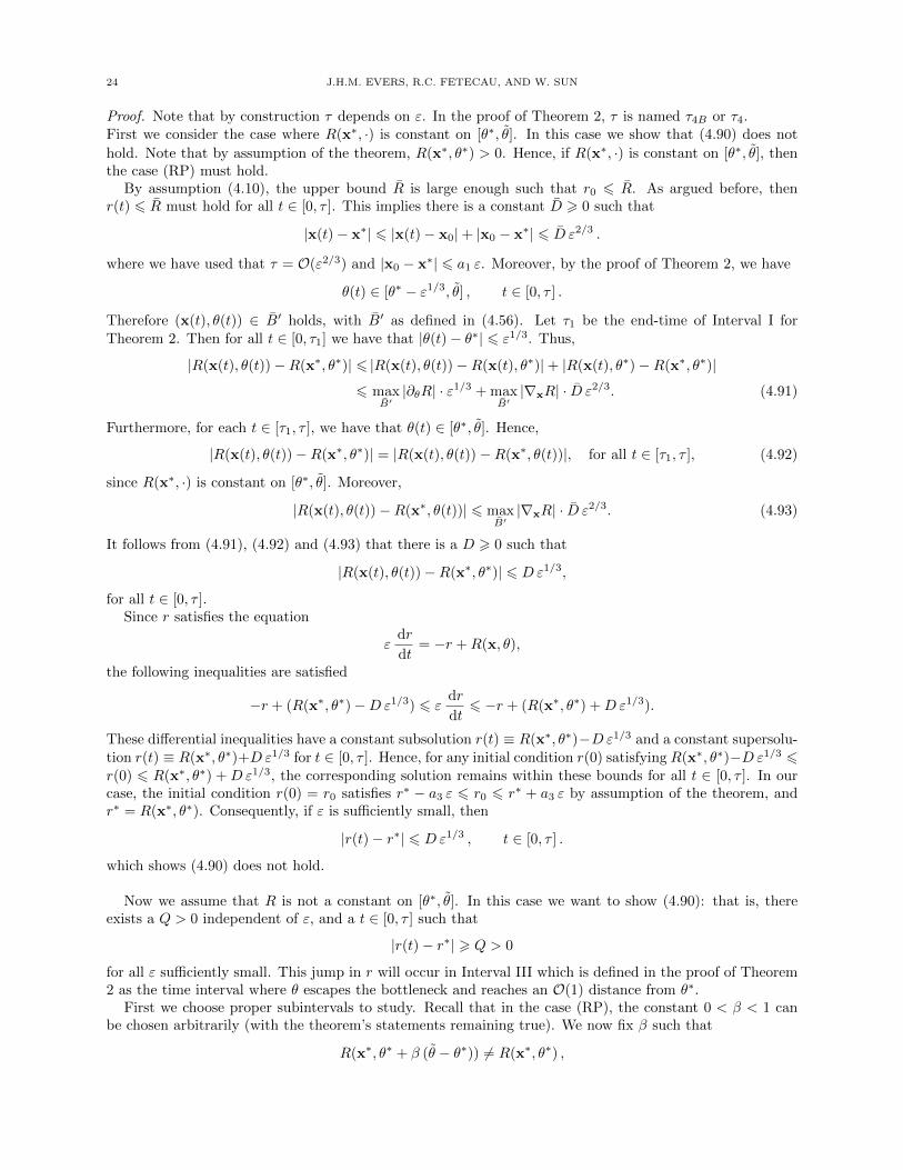
Proof. Note that by construction τ depends on ε. In the proof of Theorem 2, τ is named τ4B or τ4.First we consider the case where R(x∗, ·) is constant on [θ∗, θ]. In this case we show that (4.90) does not
hold. Note that by assumption of the theorem, R(x∗, θ∗) > 0. Hence, if R(x∗, ·) is constant on [θ∗, θ], thenthe case (RP) must hold.
By assumption (4.10), the upper bound R is large enough such that r0 6 R. As argued before, thenr(t) 6 R must hold for all t ∈ [0, τ ]. This implies there is a constant D > 0 such that
|x(t)− x∗| 6 |x(t)− x0|+ |x0 − x∗| 6 D ε2/3 .
where we have used that τ = O(ε2/3) and |x0 − x∗| 6 a1 ε. Moreover, by the proof of Theorem 2, we have
θ(t) ∈ [θ∗ − ε1/3, θ] , t ∈ [0, τ ] .
Therefore (x(t), θ(t)) ∈ B′ holds, with B′ as defined in (4.56). Let τ1 be the end-time of Interval I forTheorem 2. Then for all t ∈ [0, τ1] we have that |θ(t)− θ∗| 6 ε1/3. Thus,
|R(x(t), θ(t))−R(x∗, θ∗)| 6 |R(x(t), θ(t))−R(x(t), θ∗)|+ |R(x(t), θ∗)−R(x∗, θ∗)|
6 maxB′|∂θR| · ε1/3 + max
B′|∇xR| · D ε2/3. (4.91)
Furthermore, for each t ∈ [τ1, τ ], we have that θ(t) ∈ [θ∗, θ]. Hence,
|R(x(t), θ(t))−R(x∗, θ∗)| = |R(x(t), θ(t))−R(x∗, θ(t))|, for all t ∈ [τ1, τ ], (4.92)
since R(x∗, ·) is constant on [θ∗, θ]. Moreover,
|R(x(t), θ(t))−R(x∗, θ(t))| 6 maxB′|∇xR| · D ε2/3. (4.93)
It follows from (4.91), (4.92) and (4.93) that there is a D > 0 such that
|R(x(t), θ(t))−R(x∗, θ∗)| 6 Dε1/3,
for all t ∈ [0, τ ].Since r satisfies the equation
εdr
dt= −r +R(x, θ),
the following inequalities are satisfied
−r + (R(x∗, θ∗)−Dε1/3) 6 εdr
dt6 −r + (R(x∗, θ∗) +Dε1/3).
These differential inequalities have a constant subsolution r(t) ≡ R(x∗, θ∗)−Dε1/3 and a constant supersolu-tion r(t) ≡ R(x∗, θ∗)+Dε1/3 for t ∈ [0, τ ]. Hence, for any initial condition r(0) satisfying R(x∗, θ∗)−Dε1/3 6r(0) 6 R(x∗, θ∗) + Dε1/3, the corresponding solution remains within these bounds for all t ∈ [0, τ ]. In ourcase, the initial condition r(0) = r0 satisfies r∗ − a3 ε 6 r0 6 r∗ + a3 ε by assumption of the theorem, andr∗ = R(x∗, θ∗). Consequently, if ε is sufficiently small, then
|r(t)− r∗| 6 Dε1/3 , t ∈ [0, τ ] .
which shows (4.90) does not hold.
Now we assume that R is not a constant on [θ∗, θ]. In this case we want to show (4.90): that is, thereexists a Q > 0 independent of ε, and a t ∈ [0, τ ] such that
|r(t)− r∗| > Q > 0
for all ε sufficiently small. This jump in r will occur in Interval III which is defined in the proof of Theorem2 as the time interval where θ escapes the bottleneck and reaches an O(1) distance from θ∗.
First we choose proper subintervals to study. Recall that in the case (RP), the constant 0 < β < 1 canbe chosen arbitrarily (with the theorem’s statements remaining true). We now fix β such that
R(x∗, θ∗ + β (θ − θ∗)) 6= R(x∗, θ∗) ,

SMALL INERTIA REGULARIZATION OF AN ANISOTROPIC AGGREGATION MODEL 25
which is possible since R(x∗, ·) is not constant on [θ∗, θ]. In particular, we choose β independently of ε anddenote
ϕ2 := θ∗ + β (θ − θ∗) .
Hence in the case (RP), we have
R(x∗, ϕ2) 6= R(x∗, θ∗),
In the case (RN), the proof of Theorem 2 still works if ω∗ is taken different from (θ∗ + ϕ∗)/2, as long asω∗ is O(1) away from both θ∗ and ϕ∗. Take such ω∗ ∈ (θ∗, ϕ∗), independent of ε, such that
R(x∗, ω∗) 6= R(x∗, θ∗). (4.94)
This is possible since R(x∗, ·) is continuous and R(x∗, ϕ∗) = 0 < R(x∗, θ∗). Next, choose 0 < β < 1independent of ε such that
ϕ2 := θ∗ + β (θ − θ∗) 6 ω∗ and R(x∗, ϕ2) 6= R(x∗, θ∗).
The former is required in the proof of Theorem 2. The latter is possible by (4.94).In both cases (RP) and (RN), let
ϕ1 := θ∗ + γ (θ − θ∗)
for some 0 < γ < β independent of ε such that
θ∗ < ϕ1 < ϕ2 , R(x∗, ϕ1) 6= R(x∗, ϕ2) . (4.95)
It is possible to find such γ since R(x∗, θ∗) 6= R(x∗, ϕ2). Note that the distance between ϕ1 and ϕ2 is of
order O(1), and both quantities are O(1) away from θ∗ and θ. Moreover, within Interval III, the quantity θmoves from θ∗ + α ε1/6 to ϕ2, so for ε sufficiently small, we have:
[ϕ1, ϕ2] ⊆ Interval III,
where by an abuse of notation, we denoted by [ϕ1, ϕ2] the time interval in which θ changes from ϕ1 to ϕ2.We now study the rate of change of r with respect to θ on the subinterval [ϕ1, ϕ2]. Dividing the ODEs
for r and θ, we obtain
dr
dθ=−r +R(x, θ)1
rH(x∗, θ) + η
.
On Interval III, by (4.55) and (4.58), we have
R0 6 r(t) 6 R , |η(t)| 6 D12 ε2/3 , |R(x(t), θ(t))−R(x∗, θ(t))| 6 K1 ε
2/3
for some K1 > 0 independent of ε. Consequently, for ε sufficiently small,∣∣∣∣ dr
dθ
∣∣∣∣ =| − r +R(x, θ)||η +H(x∗, θ)/r|
62R
(K2/R)−D12 ε2/36
2R
K2/(2R)=
4R2
K2, θ ∈ [ϕ1, ϕ2] . (4.96)
where we have defined
K2 := minφ∈[ϕ1,ϕ2]
H(x∗, φ) > 0 .
The strict positivity of K2 is guaranteed by Assumption 2. Furthermore,∣∣∣∣ dr
dθ
∣∣∣∣ =| − r +R(x, θ)||η +H(x∗, θ)/r|
>| − r +R(x, θ)|
(K3/R0) +D12 ε2/3>| − r +R(x∗, θ)| −K1 ε
2/3
2K3/R0(4.97)
where K3 := maxφ∈[θ∗,θ] |H(x∗, φ)| > 0. The last inequality holds if ε is sufficiently small.
Assume that r = r(θ) changes at most o(1) on [ϕ1, ϕ2]. Then by (4.95), at least one of the quantities| − r(ϕ1) + R(x∗, ϕ1)| or | − r(ϕ2) + R(x∗, ϕ2)| must be O(1). By the uniform bound of dr/dθ in (4.96),there must therefore be an interval I of O(1) length that is either of the form I = [ϕ1, ϕ1] or of the formI = [ϕ2, ϕ2], on which it holds that
| − r(θ) +R(x∗, θ)| > K4 , θ ∈ I

26 J.H.M. EVERS, R.C. FETECAU, AND W. SUN
for some K4 > 0 independent of ε. The lower bound (4.97) subsequently implies that
|dr/dθ| > K5 > 0 , θ ∈ I
for some K5 independent of ε on the interval I. Since the length of I is of order O(1), r must have an O(1)change in I, which contradicts the assumption that r changes at most o(1) on [ϕ1, ϕ2].
Since there must be an order O(1) change in r on [ϕ1, ϕ2], it is possible to find a ϕ ∈ [ϕ1, ϕ2] and aconstant Q > 0 such that
|r(ϕ)− r∗| > Q > 0 ,
If t is the corresponding time in Interval III at which θ(t) = ϕ, then |r(t) − r∗| > Q and the statement ofthe theorem is proved. �
Remark 2. The statements of Theorems 2 and 3 still hold if we allow all particles to move, that is, ifwe consider (2.4) rather than (2.5). Note that in (2.4) the only coupling between the particles is via theirpositions; see (2.4b) and (2.4c). By assuming a uniform upper bound R for all functions Ri, one immediately
obtains a uniform bound for the speeds ri. Hence, within a time interval of O(ε2/3), all the positions xi changeby at most O(ε2/3). The analysis that follows is then similar to the case in which only one particle is moving.
5. Numerics
In this section, we first investigate the scenario presented in Figure 2.3, and also in Figure 2.2. We callthis Run 1. This is a situation where the function R1 remains strictly positive throughout our interval ofinterest; compare the case (RP) in the proof of Theorem 2. For several values of ε, we initialize the systemjust before the double root of H1 gets lost, and we examine the sharp transition of the velocity of particle 1.In particular, we measure the time it takes for θ1 to reach an order O(ε2/3) distance from θ1, and we startmeasuring at root loss. Theory predicts that this transition should take an O(ε2/3) amount of time; cf. the
statement of Theorem 2. Note that the values of θ∗1 and θ1 can be calculated a priori, once we have thefunction H1(x∗1, ·) at root loss.
In the numerical calculations, K is taken to be the Morse potential. This is the same potential as in [9]and we used the same values for the parameters. The function g is taken as in Figure 2.1(b), with parametersa = 5 and b = π.
We consider two different cases: (1) the case in which the positions of all particles are fixed, except forthe one that undergoes the change in velocity; and (2) the case in which all four particles are evolving duringthe transition interval. The results are presented in Figure 5.1. In both cases, a linear fit shows that, upto a small numerical error, the amount of time needed for θ1 to make the transition scales as ε2/3. For thecase where only particle 1 is moving, this is in agreement with exactly what was proven in Theorem 2. InRemark 2 we argued that the statement of Theorem 2 also holds if all particles are allowed to evolve. Thelinear fit through the diamonds in Figure 5.1 supports this result and provides the correct scaling.
Next, we take the same number of particles (i.e. 4) and the same parameters, but a different initialconfiguration. Call this Run 2. We consider a scenario that leads to root loss in one of the particles (in this
case, particle 2), while the function R2(x∗2, ·) is negative in a subinterval of [θ∗2 , θ2]; cf. the case (RN) in theproof of Theorem 2. The spatial coordinate x∗2 is such that H2(x∗2, ·) has a double root. In particular, this
double root occurs at θ = θ∗2 , while a simple root is present at θ2 > θ∗2 , where the derivative of H2(x∗2, ·) isnegative. See Figure 5.2; the insert is included to show that R2(x∗2, θ
∗2) > 0.
In Figure 5.3 we show that the angle and the absolute value of the velocity of particle 2 both make asharp transition in Run 2. We present numerical results for ε = 10−2, 10−3, and 10−4. For decreasing ε,the plots exhibit similar behaviour as in Figures 2.3(b) and 2.3(c). Note that in Figure 5.3(b) a logarithmicscale is used on the vertical axis.
For Run 2, we investigate in Figure 5.4 how the length of the transition interval scales with ε. As wedid for Run 1, we measure the time from root loss until θ2 reaches an O(ε2/3) distance from θ2. Numericalcalculations were done for the case in which only particle 2 moves, as well as for the case in which all fourparticles move. In both cases, the linear fit in Figure 5.4 shows that θ2 needs an order O(ε2/3) amount oftime to make the transition. This is in agreement with Theorem 2 and Remark 2.

SMALL INERTIA REGULARIZATION OF AN ANISOTROPIC AGGREGATION MODEL 27
ϵ10-6 10-5 10-4
time
inte
rval
10-4
10-3
10-2
τ, one movingfit, slope=0.676τ, all movingfit, slope=0.679
Figure 5.1. The amount of time τ it takes in Run 1 from root loss until reaching |θ1 − θ1| = ε2/3, plotted
as a function of ε. Circles: Numerical calculations corresponding to (2.5). That is, we focus on particle 1
whose velocity undergoes the fast transition. All other particles have their positions fixed. The slope of thefitted line is approximately 2
3, which is in agreement with Theorem 2, where the transition time interval
is proved to be O(ε2/3). Diamonds: Numerical calculations corresponding to (2.4), where again particle 1
undergoes a fast transition in velocity, but all particles’ positions evolve during the transition interval. Theslope of the fitted line is approximately 2
3, which supports the claim in Remark 2 that Theorem 2 predicts
the correct length of the transition interval also when all particle positions evolve.
Because the two datasets are nearly overlapping, in the plot the circles (and the corresponding linear fit)have been translated upwards; it is only the slope that we are interested in.
θ0.5 1 1.5 2 2.5 3 3.5 4
0
0.1
0.2
0.3
0.4
0.5
0.6
0.7
0.8
θ∗2 θ2
H2(θ) at t*R2(θ) at t*
1.28 1.3 1.32
×10-3
0
2
Figure 5.2. The function H2 associated to particle 2 (solid black line), drawn as a function of θ at the
breakdown time t = t∗ of Run 2. A double root is present at θ∗2 ≈ 1.30 (filled circle). The open circle
indicates θ2 ≈ 3.71, where H2 has a single root and the derivative is negative. Note that R2 is negative in
a subinterval of [θ∗2 , θ2], but R2(θ2) > 0. The insert shows the graph near θ∗2 in the last numerical timestep
in which a root of H2 is present there. The root is still a simple root; the actual double root is very hard tocapture numerically, in particular because the graph of H2 is very shallow in that region. The aim of theinsert, however, is to show that R2 is strictly positive (be it small) near θ∗2 .
Appendix A. Sketch of Proof of Theorem 1
In this appendix we briefly explain the proof of Theorem 1. As mentioned before, the proof parallels thatfor Theorem 2 with r constant.
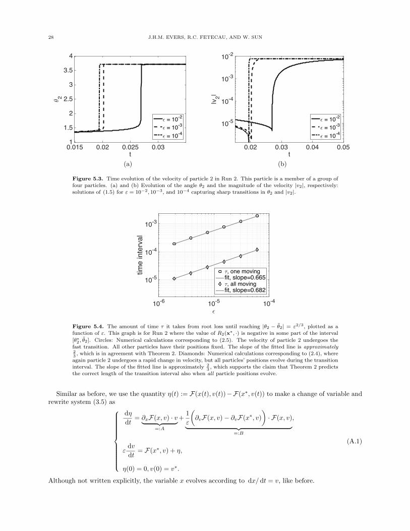
28 J.H.M. EVERS, R.C. FETECAU, AND W. SUN
t0.015 0.02 0.025 0.03
θ 2
1
1.5
2
2.5
3
3.5
4
ϵ = 10-2
ϵ = 10-3
ϵ = 10-4
t0.02 0.03 0.04 0.05
|v2|
10-5
10-4
10-3
10-2
ϵ = 10-2
ϵ = 10-3
ϵ = 10-4
(a) (b)
Figure 5.3. Time evolution of the velocity of particle 2 in Run 2. This particle is a member of a group offour particles. (a) and (b) Evolution of the angle θ2 and the magnitude of the velocity |v2|, respectively:
solutions of (1.5) for ε = 10−2, 10−3, and 10−4 capturing sharp transitions in θ2 and |v2|.
ϵ10-6 10-5 10-4
time
inte
rval
10-5
10-4
10-3
τ, one movingfit, slope=0.665τ, all movingfit, slope=0.682
Figure 5.4. The amount of time τ it takes from root loss until reaching |θ2 − θ2| = ε2/3, plotted as a
function of ε. This graph is for Run 2 where the value of R2(x∗, ·) is negative in some part of the interval
[θ∗2 , θ2]. Circles: Numerical calculations corresponding to (2.5). The velocity of particle 2 undergoes the
fast transition. All other particles have their positions fixed. The slope of the fitted line is approximately23
, which is in agreement with Theorem 2. Diamonds: Numerical calculations corresponding to (2.4), where
again particle 2 undergoes a rapid change in velocity, but all particles’ positions evolve during the transition
interval. The slope of the fitted line is approximately 23
, which supports the claim that Theorem 2 predictsthe correct length of the transition interval also when all particle positions evolve.
Similar as before, we use the quantity η(t) := F(x(t), v(t))−F(x∗, v(t)) to make a change of variable andrewrite system (3.5) as
dη
dt= ∂xF(x, v) · v︸ ︷︷ ︸
=:A
+1
ε
(∂vF(x, v)− ∂vF(x∗, v)
)· F(x, v)︸ ︷︷ ︸
=:B
,
εdv
dt= F(x∗, v) + η,
η(0) = 0, v(0) = v∗.
(A.1)
Although not written explicitly, the variable x evolves according to dx/ dt = v, like before.

SMALL INERTIA REGULARIZATION OF AN ANISOTROPIC AGGREGATION MODEL 29
There are two powers of ε in Theorem 1: the length of the time interval for the transition from v∗ to v tooccur and the final distance of v to v.
Interval I. The overall time scale is determined by Interval I, where A dominates B and F(x∗, v) becomescomparable to η. In this interval, we have
|x(t)− x∗| = O(t) , η(t) = O(t) .
Moreover, η is the main driving force of v. Hence,
|v − v∗| = O(t2
ε
).
The balance of F(x∗, v) with η then gives
(v − v∗)2k ∼ t ⇒(t2/ε
)2k ∼ t ⇒ t = O(ε2k/(4k−1)) , (A.2)
which gives the overall transition time scale. Denote by time τ1 the end of Interval I. Then we have
v(τ1)− v∗ = O(ε1/(4k−1)
),
Note that in the case where k = 1, that is, we have the double-root loss as in Section 3.1 or Section 4, werecover the time scale O(ε2/3). Moreover, v(τ1)− v∗ = O
(ε1/3
), cf. (4.15).
Interval II. In Interval II we use that A is still positive and dominates B, which implies that η remainspositive. In Interval II we have moreover that F(x∗, v) ∼ (v − v∗)2k. Therefore,
εd(v − v∗)
dt& (v − v∗)2k,
with initial condition
v(τ1)− v∗ = O(ε1/(4k−1)
).
It follows that
v(t)− v∗ &(
ε
ε2k/(4k−1) − C (t− τ1)
)1/(2k−1)
,
for some constant C; compare (4.49). By taking t := τ2 = τ1 +O(ε2k/(4k−1))−O(ε(4k+1)/(2(4k−1))), we findthat
v(τ2)− v∗ & ε(4k−3)/(2(2k−1)(4k−1)). (A.3)
This distance is (slightly) larger than the one at the end of Interval I. It turns out that v(τ2) is actually farenough from v∗ to guarantee that v will not remain trapped in the bottleneck. We will see this in the nextinterval.
For the case k = 1, the orders of magnitude are τ2 = τ1 +O(ε2/3)−O(ε5/6) and v(τ2)− v∗ & ε1/6. Thesecorrespond to (4.39) and the first equation in (4.41).
Interval III. In Interval III we allow A+B (and hence η) to become negative. This is the interval in whichv reaches an O(1) distance from v∗.
In this interval η may be negative, but it is still small: |η| . ε2k/(4k−1). Consequently,
εd(v − v∗)
dt& (v − v∗)2k −O(ε2k/(4k−1)),
with initial condition satisfying (A.3). Due to this initial condition, (v − v∗)2k initially dominates theO(ε2k/(4k−1)) term. It follows that v increases throughout the interval and the term (v − v∗)2k remains thedominant one. Therefore, the second term can be absorbed into the first one, to obtain
d(v − v∗)dt
& ε−1 (v − v∗)2k. (A.4)
Compare this inequality, for the case k = 1, to (4.60). This is the same estimate as in Interval II, but theinitial condition is different. Taking (A.3) into account, we find
v(t)− v∗ &(
ε
ε1−(4k−3)/(2(4k−1)) − C (t− τ2)
)1/(2k−1)
, (A.5)
30 J.H.M. EVERS, R.C. FETECAU, AND W. SUN
for some constant C. This guarantees that in a time interval after τ2 of O(ε(4k+1)/(2(4k−1)))−O(ε) length,v moves an O(1) distance away from v∗. We remark that if k = 1 we have the same timescales as in (4.53).
Interval IV. The final distance of v to v is determined in Interval IV, where v starts O(1) away from bothv∗ and v and the main driving force for v is F(x∗, v). More precisely, it is the term (v − v)2`−1 in F(x∗, v);see (3.6). Over this interval, we have
|x(t)− x∗| = O(ε2k/(4k−1)
), η(t) = O
(ε2k/(4k−1)
).
Consequently,
εd(v − v)
dt& −(v(t)− v)2`−1 −O
(ε2k/(4k−1)
). (A.6)
Note that −(v(t) − v)2`−1 is positive, since (v(t) − v)2`−1 is an odd power of a negative quantity, hencenegative. If k = ` = 1, then (A.6) is the analogue of (4.89) in the proof of Theorem 2.
Since (v− v) is O(1) initially, we can absorb the −O(ε2k/(4k−1)
)term into the positive term −(v− v)2`−1,
until they balance. That point in time marks the end of our interval of consideration, and it is the size of ηthat determines |v − v| at the end.
The driving mechanism in this interval is
εd(v − v)
dt& −(v − v)2`−1 .
The subsequent step is based on differential inequalities (like before), but it requires a separate approach for` = 1 and for ` > 1. The resulting inequalities yield that at the end of Interval IV, we have
|v − v| = O(ε(2k)/(4k−1)
)if ` = 1, and |v − v| = O
(ε(2k−1)/((4k−1)(2`−1))
)if ` > 1.
The powers of ε in terms of k, ` show that in general the larger k is, the more time it takes the systemto leave the bottleneck that is present around v∗. Moreover, if ` increases, then the graph of F becomes“flatter” near v. In the theorem, this is expressed by the fact that ν decreases and thus the final distancebetween v and v is larger. If k = ` = 1 then we have exactly |v− v| = O
(ε2/3
)as we have in Theorem 2 for
|θ− θ|. The order of magnitude of Interval IV is arbitrarily close to O(ε). That is, the length is O(ε1−λ) forarbitrarily small λ > 0, similar to Interval IV in the proof of Theorem 2. We omit further details here.
References
[1] D. Balague, J.A. Carrillo, T. Laurent, and G. Raoul, Dimensionality of local minimizers of the interaction energy, Arch.
Ration. Mech. Anal. 209 (2013), no. 3, 1055–1088.[2] M. Ballerini, N. Cabibbo, R. Candelier, A. Cavagna, E. Cisbani, I. Giardina, V. Lecomte, A. Orlandi, G. Parisi, A.
Procaccini, M. Viale, and V. Zdravkovic, Interaction ruling animal collective behaviour depends on topological rather than
metric distance: evidence from a field study, Proc. Natl. Acad. Sci. 105 (2008), 1232–1237.[3] A.L. Bertozzi and T. Laurent, Finite-time blow-up of solutions of an aggregation equation in Rn, Comm. Math. Phys.
274 (2007), no. 3, 717–735.
[4] A.L. Bertozzi, T. Laurent, and J. Rosado, Lp theory for the multidimensional aggregation equation, Comm. Pur. Appl.Math. 64 (2011), no. 1, 45–83.
[5] M. Bodnar and J.J.L. Velazquez, Derivation of macroscopic equations for individual cell-based models: a formal approach,
Math. Meth. Appl. Sci. 28 (2005), no. 15, 1757–1779.[6] , An integro-differential equation arising as a limit of individual cell-based models, J. Differential Equations 222
(2006), no. 2, 341–380.[7] S. Camazine, J.-L. Deneubourg, N.R. Franks, J. Sneyd, G. Theraulaz, and E. Bonabeau, Self-Organization in Biological
Systems, Princeton Studies in Complexity, Princeton University Press, Princeton, NJ, 2003. Reprint of the 2001 original.
[8] J.A. Carrillo, M. DiFrancesco, A. Figalli, T. Laurent, and D. Slepcev, Global-in-time weak measure solutions and finite-timeaggregation for nonlocal interaction equations, Duke Math. J. 156 (2011), 229–271.
[9] J.H.M. Evers, R.C. Fetecau, and L. Ryzhik, Anisotropic interactions in a first-order aggregation model, Nonlinearity 28(2015), 2847–2871.
[10] J.H.M. Evers, A. Muntean, and A.A.F. van de Ven, Crowds reaching targets by maximizing entropy: a Clausius-Duhem in-
equality approach, Proceedings of the 1st IFAC Workshop on Control of Systems Governed by Partial Differential Equations,
2013, pp. 263–268.[11] R.C. Fetecau, Y. Huang, and T. Kolokolnikov, Swarm dynamics and equilibria for a nonlocal aggregation model, Nonlin-
earity 24 (2011), no. 10, 2681–2716.[12] R.C. Fetecau and W. Sun, First-order aggregation models and zero inertia limits, J. Differential Equations 259 (2015),
6774–6802.
SMALL INERTIA REGULARIZATION OF AN ANISOTROPIC AGGREGATION MODEL 31
[13] R.C. Fetecau, W. Sun, and C. Tan, First-order aggregation models with alignment, Phys. D 325 (2016), 146–163.[14] L. Gulikers, J.H.M. Evers, A. Muntean, and A.V. Lyulin, The effect of perception anisotropy on particle systems describing
pedestrian flows in corridors, Journal of Statistical Mechanics: Theory and Experiment (2013), P04025.
[15] D. Helbing and P. Molnar, Social force model for pedestrian dynamics, Phys. Rev. E 51 (1995), no. 5, 4282–4286.[16] M.H. Holmes, Introduction to Perturbation Methods, 2nd ed., Texts in Applied Mathematics, vol. 20, Springer New York,
2013.
[17] M. O. Jackson, Social and Economic Networks, Princeton University Press, 2010.[18] M. Ji and M. Egerstedt, Distributed coordination control of multi-agent systems while preserving connectedness, IEEE
Trans. Robot. 23 (2007), no. 4, 693–703.[19] T. Kolokolnikov, H. Sun, D. Uminsky, and A.L. Bertozzi, Stability of ring patterns arising from two-dimensional particle
interactions, Phys. Rev. E, Rapid Communications 84 (2011), 015203(R).
[20] H. Kunz and C.K. Hemelrijk, Simulations of the social organization of large schools of fish whose perception is obstructed,Appl. Anim. Behav. Sci. 138 (2012), 142–151.
[21] A.J. Leverentz, C.M. Topaz, and A.J. Bernoff, Asymptotic dynamics of attractive-repulsive swarms, SIAM J. Appl. Dyn.
Syst. 8 (2009), no. 3, 880–908.[22] S. Motsch and E. Tadmor, Heterophilious dynamics enhances consensus, SIAM Review 56 (2014), 577–621.
[23] J.K. Parrish and L. Edelstein-Keshet, Complexity, pattern, and evolutionary trade-offs in animal aggregation, Science 284
(1999), 99–101.[24] R. Seidl and W. Kaiser, Visual field size, binocular domain and the ommatidial array of the compound eyes in worker
honey bees, J. Comp. Physiol. A 143 (1981), 17–26.
[25] G. Theraulaz, J. Gautrais, S. Camazine, and J.-L. Deneubourg, The formation of spatial patterns in social insects: fromsimple behaviors to complex structures, Phil. Trans. R. Soc. Lond. 361 (2003), 1263–1282.
[26] A. N. Tikhonov, Systems of differential equations containing small parameters in the derivatives, Mat. Sb. (N.S.) 31(73)(1952), 575–586.
[27] A.B. Vasil′eva, Asymptotic behaviour of solutions of certain problems for ordinary non-linear differential equations with
a small parameter multiplying the highest derivatives, Uspekhi Mat. Nauk 18 (1963), no. 3(111), 15–86.[28] J.H. von Brecht and D. Uminsky, On soccer balls and linearized inverse statistical mechanics, J. Nonlinear Sci. 22 (2012),
no. 6, 935–959.
Department of Mathematics and Statistics, Dalhousie University, PO Box 15000, Halifax, NS B3H 4R2, Canada,
& Department of Mathematics, Simon Fraser University, 8888 University Dr., Burnaby, BC V5A 1S6, CanadaE-mail address: [email protected]
Department of Mathematics, Simon Fraser University, 8888 University Dr., Burnaby, BC V5A 1S6, CanadaE-mail address: [email protected]
Department of Mathematics, Simon Fraser University, 8888 University Dr., Burnaby, BC V5A 1S6, CanadaE-mail address: [email protected]